The Peñalara Mountain Meteorological Network (1999–2014): Description, Preliminary Results and Lessons Learned


1
Centro de Investigación, Seguimiento y Evaluación Sierra de Guadarrama, Rascafría 28740, Spain
2
InterMET Sistemas y Redes S.L.U., Cea Bermudez 14B-6C, Madrid 28003, Spain
3
Facultad Ciencias Ambientales y Bioquímica, Universidad de Castilla-La Mancha (UCLM),Avda Carlos III s/n, Toledo 45071, Spain
*
Author to whom correspondence should be addressed.
Atmosphere 2017, 8(10), 203; https://doi.org/10.3390/atmos8100203
Submission received: 7 July 2017
/
Revised: 31 August 2017
/
Accepted: 12 October 2017
/
Published: 17 October 2017
(This article belongs to the Special Issue Atmospheric Processes over Complex Terrain)
Abstract
:This work describes a mountain meteorological network that was in operation from 1999 to 2014 in a mountain range with elevations ranging from 1104 to 2428 m in Central Spain. Additionally, some technical details of the network are described, as well as variables measured and some meta information presented, which is expected to be useful for future users of the observational database. A strong emphasis is made on showing the observational methods and protocols evolution, as it will help researchers to understand the sources of errors, data gaps and the final stage of the network. This paper summarizes mostly the common sources of errors when designing and operating a small network of this kind, so it can be useful for individual researchers and small size groups that undertake a similar task on their own. Strengths and weaknesses of some of the variables measured are discussed and some basic calculations are made in order to show the potential of the database and to anticipate future deeper climatological analyses over the area. Finally, the configuration of an automatic mountain meteorology station is suggested as a result of the lessons learned and the the common state of the art automatic measuring techniques.
Keywords:
mountains; observations; network; validation; uncertainties; climate; snow; extreme conditions1. Introduction
Despite the importance of mountains to the local to regional climate, meteorological observations in mountains were not intensively made until the mid-nineteenth century. Since then, and mostly in recent decades, progress in conducting continuous observations has been made by using standardized methods, but there are still some uncertainties which are difficult to solve [1,2]. The very specific conditions of mountain environments make them excellent indicators of climate change, [3,4,5,6,7,8,9,10,11]. Nevertheless it is commonly accepted that a better understanding of the climatic characteristics of mountain regions is limited by a lack of observations adequately distributed in time and space.
There are several reasons that explain this persistent lack of reliable and long term meteorological observations in mountains. Remoteness, extreme environmental conditions, difficulties on having powerful energy sources, and reliable telecommunication are the main reasons. On the other hand, due to the high spatial variability of the meteorological fields in mountains [12], a mountain observatory is normally only representative of a very small area. This makes the need for a higher density of stations in mountains more necessary than at lower elevations, increasing the overall cost of installation and operation.
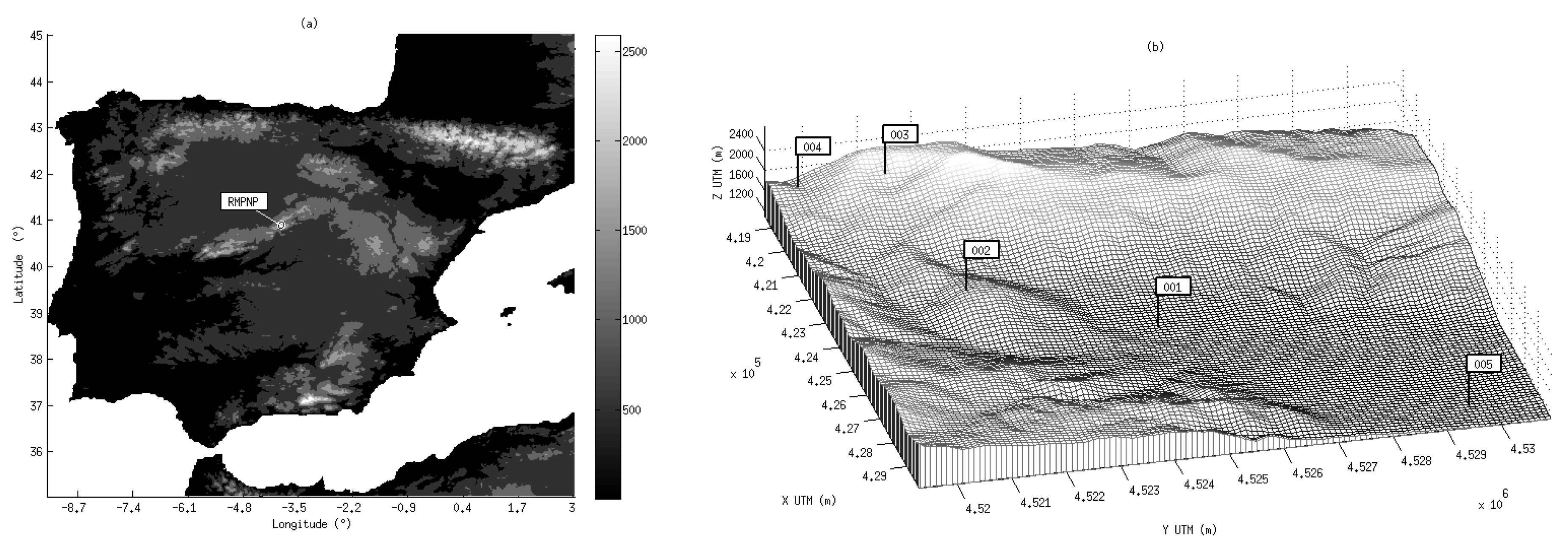
Peñalara Massif is located in Sierra de Guadarrama, which is part of the Iberian Central System [13]. This mountain range lies over two extensive plateaus in the center part of the Iberian Peninsula and shows excellent conditions for conducting weather and climate observations since it has been kept relatively unaltered (Figure 1a). Due to a concatenation of circumstances, this area has been kept away from urban pressure and so it has been recently included in the Spanish National Park Network. Land use, dominated by natural forests and alpine grassland mixed with bare rock at higher altitudes, has remained almost the same over the last centuries. This area is crucial for the sustainability of the region in terms of water resources and could be an excellent observatory for conducting regional climatological research. Due to the high altitude of the area and its exposure to the free troposphere, it could also serve as an indicator of higher scale meteorological phenomena. On the other hand, urban development and its associated pollution activities have increased since the 80’s at the adjacent regions. For example, the Madrid Metropolitan Area, which is at a horizontal distance of 50 km and with a mean altitude difference of 1600 m, is surely affecting its air composition under certain situations. This area is characterized by an alpine climate located in a continental Mediterranean system. Mean values of temperature and precipitation are comparable to other mountain areas in southern Europe, but with some characteristics like a severe summer drought and a high inter-annual variability [14]. Precipitation occurs mainly due to large and synoptic scale precipitation phenomena but with a marked orographic enhancement [15].
In recent years, this area has been subject to numerous scientific and multidisciplinary studies, such as in geomorphology [16,17,18,19,20], limnology [21,22,23], ecology [24], zoology [25,26,27,28], botanics [29,30,31,32,33,34,35,36,37,38,39,40] and meteorology and climate [7,14,15,18,41,42,43,44,45,46,47,48].
This area, also known as Peñalara Natural Park, has always been the subject of research programs that demand local meteorological observations. Some of these projects had their own measurements, but they were interrupted when the project was finished or when observations were too target specific. In order to provide quality data for broader scientific activities that were conducted in the area, the Park decided to start making their own observations in 1998. A long time perspective, scientific quality equipment, open access of data and good data completion were the guidelines of the incipient network.
The installation of one of the first fully automatic meteorological stations above 2000 m.a.s.l. in the Iberian Peninsula was followed by the installation of other four automatic meteorological stations shaping what was formally known as Red Meteorológica del Parque Natural de Peñalara (RMPNP hereafter) (Figure 1b). Data is now freely available by request to Centro de Centro de Investigación, Seguimiento y Evaluación del Parque Nacional Sierra de Guadarrama (https://www. parquenacionalsierraguadarrama.es/es/administracion/directorio/cise).
This work aims at describing the design, operation and results of this Peñalara Mountain Meteorological Network. It includes meta data information that might be useful for future users of the database. Also, some preliminary analysis has been performed in order to show the potential of the database. These results are one of the first climatic results of the area and hopefully will trigger further research in the future. Special attention is paid explaining the technical and operational procedures since they might be helpful to other groups that are starting to carrying out meteorological observations in the mountains.
Some of the lessons learned, since the first installation in 1999, are summarized here and were the keystone for a full ongoing renewal of this network [49].
This paper is organized as follows. First, the method used for the design and installation of the network is described. It also includes some details of the organization, maintenance procedures, quality assurance program, and a description of the sites and some discussion about the strengths and weaknesses of the observational database. The last section includes the conclusions and future lines of research.
2. Method
Since 1998, the number of observatories in the area was increased in order to take into account the complexity of the area and the resources available. The installation process followed a time sequence, shown in Table 1, and follows a measuring strategy that is explained in the next sections. Finally, the network consisted of five automatic weather stations, one manual observatory and some fixed sites for ancillary measurements and prototype testing (Figure 1b).
2.1. Measuring Objective
The objective of a meteorological network determines its design and configuration since depending on the potential uses of the data, different network designs are possible and valid [50].
The main objective of this network was to obtain meteorological data representative of Peñalara Massif and the area of influence that would help to expand the current knowledge of its environment and more specifically of its weather phenomena and climate at the local and regional level, trying to keep the associated unavoidable uncertainties to a minimum.
2.2. Measuring Strategy
Special care was taken to define a measuring strategy that would allow for controlling all the factors that affect the objective of the network. Aspects that were considered are: measuring technique (manual or automatic), instrumentation used (quality of the sensors, calibration, sample time, averaging time), exposure (macro-scale and micro-scale sitting criteria), and maintenance protocols (data handling, collection intervals, post-processing and storage) [51]. The following sections summarize the measuring strategy that was finally adopted.
2.2.1. Measuring Technique
Automatic measurements were the base of this network. Additional manual measurements for calibration and data quality control were intensively performed in parallel at one site and punctual manual measurements were performed during maintenance.
2.2.2. Density of Stations
Considering the size and orographic complexity of the area, up to five sites were finally installed to cover the elevation, which ranged from 1102 m.a.s.l. to 2079 m.a.s.l.. Since the highest point of the area was 2414 m.a.s.l., this made an average of one site per 260 m of altitude. The density of stations was higher at higher altitudes. This number of stations was considered optimum in terms of the maximum number of sites that could be maintained with a reasonable level of performance.
2.2.3. Sitting Criteria
Recommendations from the World Meteorological Organization [52] were followed where and whenever it was possible, but the following specific difficulties had to be taken into consideration:
2.2.4. Remoteness
Remoteness is one of the main sources of data gaps and measuring errors. Installations were carefully planned due to the complex logistics and the narrower range of options for materials and structures that could be used due to environmental restrictions. A preventive maintenance program was planned; however, due to various factors, it was difficult to achieve an optimum level of maintenance. This led to an increased vulnerability to extreme weather conditions, fauna and vandalism. Different transmission methods were tested: first manual downloading from 1999 to 2005, and with the advent of GPRS after 2008, satisfactory data completion, higher than 90%, could be accomplished (Table 1). We found that remoteness was closely related to maintenance costs.
2.2.5. Extreme Environmental Conditions
Since temperatures can remain low for several days at these sites, a proper solar power source was finally achieved by using larger solar panels and gel batteries which are more efficient at lower temperatures. Other sources, like wind power, were not considered due to environmental restrictions. Rugged sensors were chosen and special attention was taken to build robust structures and sensor booms while trying to minimize the environmental impact. Some standard measuring heights were not followed since they would have decreased the robustness of the whole site and would also have made replacing the sensors more difficult. This was the case for the 10 m height established for wind, which was only possible at very few sites.
2.2.6. Microclimate
Due to the complex orography a great variety of microclimates were expected. Special care was taken not to select locations under the influence of particular conditions, such as: obstacles, projected shades, air stagnation, cold pools, and other local effects. This was sometimes difficult to achieve and possible sources of interference were documented (Table 2).
2.2.7. Safety and Environment
This area can be risky for maintenance personnel, especially in winter, so this also played a role in the final decision of the site selection. Higher precautions were taken in order to minimize the environmental visual impact of towers, sensors and equipment since this area has a high degree of environmental protection.
2.3. Quality Assurance and Quality Control
The quality assurance program which was finally adopted was the result of a continuous evolution through the years thanks to the gain of knowledge. During the first years of operation most of the resources available were invested in the installation of new sites and the consolidation of the network. Later, an appropriate maintenance program was necessary in order to improve the completion of data, as can be seen in Table 2. Once a sustainable maximum number of stations was reached, efforts were focused on improving the quality of the observations. Figure 2 summarizes dataflow and illustrates the different procedures finally adopted.
One of the first things to take into account was to guarantee that the sensors had a valid certificate of calibration. Following the instructions from the manufacturers, periodical replacement of temperature/ humidity and wind sensors was performed. Data loggers were replaced three times during this period and there was a continuous renovation of the structures, cabinets and solar panels.
Nevertheless, other factors that were considered that could have a higher impact on the uncertainty of the observations. From the experience gained, we can state that during certain winter conditions it was difficult to guarantee that the sensor was correctly exposed to the measuring device. Some examples are the distance to the ground which changes due to snow accumulation, obstacles that project rain shadows on sensors, wind affecting rain catchment due to aerodynamic effects (underestimation), wind turbulence anticipating the tipping of the bucket at the rain gauges (overestimating), snow blocking pyrometers windows and non-heated rain gauges. All these errors could have been acceptable if they were random, not very frequent nor detectable, but, on the contrary, they were dependent on weather factors, adding unacceptable biases for long term climatological analyses and they were difficult to detect. In order to partially solve this, a validation process was developed using automatic tests, but expert judgment played the most important role in this issue. Regarding long time drift and homogeneity, Alexandersson tests [53] were calculated to the longest time series but more efforts will have to be made in the future. Recommendations like the MeteoMET project [54] will be considered in the future, especially the solution based on in situ calibration that would account for all the measurement chain errors.
The following sections describe the main features of the QAQC finally adopted.
2.3.1. Preventive Maintenance
Regular visits to the sites, before any problem was detected, were conducted. The average frequency of these visits was established between one and two months, depending on the weather conditions and resources available. Preventive maintenance included cleaning panels and sensors, structures checking, parallel manual measurement for checks of performance and extension of calibration times given by the manufacturer. On site rain gauge calibration was performed once a year using a rain gauge calibrator. Electrical and telecommunications checks were also performed. All these tasks were recorded in a control chart.
2.3.2. Corrective Maintenance
Repairs of a malfunctioning part of a station were often necessary. Sometimes it required a prior visit for diagnostic and evaluation of damages. Corrections were made in an expedient manner in order to minimize data loss, but it depended on the availability of spare parts and weather conditions. It was often decided that if a sensor broke during wintertime, it would not be replaced until the following spring.
2.3.3. Data Validation
During the data validation procedure, determinations were made as to whether an observation was valid to be included in the time series data [55]. This was developed in order to make it easier for users not directly involved in the management of the network to use the data, as well as giving a certain guarantee of acceptable uncertainty with respect to a general scientific purpose.
Original data was always kept for advanced users to apply their own criteria according to their objectives. This process was done following a two phase protocol. A first level validation was done almost in real-time during the importing process. The objective of this phase was to detect impossible values, outliers and very clear malfunctions. After 2008, reliable telecommunication with remote sites was available so it was possible to do more frequent data downloading and perform the first phase of validation almost at real time. This made it possible to trigger alarms for corrective maintenance and have additional criteria for experts’ assessment in phase two. The second-phase of validation was made off-line, when information from all sites was already collected, maintenance reports were finished and observations from other networks were available. This phase was conducted every three months. At this phase, climatological site specific thresholds were used and internal consistency tests were performed. Spatial coherence tests using information from neighboring stations and data from other networks or reanalysis were made yearly. In this phase, expert review confirmed the results of the first automatic phase validation. Once a year, long term drift tests were also performed for the long time series. As a result of this process, data was individually tagged with the following codes: V: valid data, D: not valid data, C: corrected data and T: temporal not validated data. At this point, the data was ready for dissemination.
2.3.4. Storage and Reporting
As long as the volume of data increased with new data, variables and sites, the storage technology became critical (Table 1). Data storage evolved from individual ASCII (American Standard Code for Information Interchange) files during the first years to spreadsheets with some automatic statistic calculations to finally a PostgreSQL based database ([56]; PostgreSQL Global Development Group, 1996–2014). A PHP [57] graphical user interface accessible remotely through the web was developed for data storage, validation and reporting to users, the public and organizations. Validation and graphics routines were programed with Python [58]. The last evolutions of this software relied more on Python and newer versions of PosgreSQL.
3. Results and Discussion
RMPNP consisted of five automatic meteorological stations that covered the area of Massif of Peñalara and the lower lands of Valle del Lozoya (Figure 1b). Additionally, a manual observatory of temperature and precipitation was installed near one of the automatic sites for calibration purposes and research. The following sections describe some characteristics of the sites that future data users might find relevant for their application. Also, some discussions about the possible sources of the uncertainty of temperature, wind and precipitation data are shown.
3.1. Description of the Network
Table 3 shows the RMPNP code, name, coordinates, starting year, codification of variables, magnitudes measured and the sensors currently used. Even though the location of the sites has been chosen to be as representative as possible following the sitting criteria already mentioned, sometimes this was difficult in this mountainous area. Table 2 includes some general comments about the factors that might affect the representativeness of each individual site. Metadata information has been taken and archived. Such information should always be taken into account before using this observational database [59]. The brief information shown in Table 2 should not substitute an in situ visit of the site, something that is always recommended before using the data.
Since the installation of the first stations (Zabala and Cabeza Mediana) in 1999 this network has experienced a set of changes as a result of technological evolution and knowledge improvements [41]. Regarding changes in sensor and data logging system technology, the evolution has been less marked than in telecommunications and quality assurance procedures. Data logging was performed first by using a NRG9000 data logger (renewablenrgsystems.com). With the generalization of GSM (Global System for Mobile communications), loggers were progressively substituted with Gantner IDL101 loggers (gantner-instruments.com) and a Wavecom (sierrawireless.com) modem was used for data transfer.
Table 1 shows the annual temperature data completeness for all stations. It could be used as a good estimator of the performance of the stations since this variable has shown to be very robust throughout all this period. Lower results show problems related to power failures, general malfunction due to a general breakage of the stations and also human errors. This table shows also the increment of data volume through the years and the technology change that the network has suffered from its first years to the present, especially in relation to telecommunications and data storage systems. Before 2005, data collection was made through in situ access to the sites walking and downloading data directly from the logger to a portable computer. This method was proven to be very robust since power requirements of the systems were very low and loggers could be operated by small power panels and batteries. This option should not be discounted for very remote networks, but data completion is more difficult to achieve as it has been shown here. With more sites to be maintained after 2008, this was unsustainable, affecting data completion (Table 1). GSM opened a new horizon, since stations could be accessed remotely for data downloading, configuration and status control. However, poor signal quality in these mountains and problems due to a still incipient technology with few automation software possibilities made this technology fairy unreliable. GPRS (General Packet Radio Service) and the evolution of GSM oriented to data transfer through the cellular network was the ultimate solution that gave the needed reliability to the communications at RMPNP. Telecommunication not only gave the possibility of having data at the desktop, saving man power and resources, but also made it possible to have an almost on line diagnostic of the station status. It really made a difference on data completeness and compensated for the extra work due to the increased number of sites (Table 1).
Another important technological advancement was the way data was stored. With the first two stations and during the first years, individual ASCII was simple and useful (Table 1). Nevertheless, tagging data individually was soon found to be necessary as a result of the QAQC process and ASCII files not being ideal. This was first solved by using spreadsheets which also offered an easy solution for some statistical calculations, wind roses and daily and monthly time series using macros. However, again, it turned in being too impractical considering the rapid increment of the volume of data needed to be stored (Table 1). The solution was found by using the PosgreSQL database environment, which brought new possibilities and saving man power. This made the use of functions and algorithms programmed in Python for data validation, the automation of reports and the exchange of information with third parties easier. Also, it gave reliability to the system thanks to the powerful capabilities of this environment for backups and remote access for easier management.
In order to illustrate the strengths and weaknesses of this observational database, we discuss the possible sources of uncertainty of the data along with some basic analyses in the following subsections. These simple calculations do not intend to be an exhaustive overview of the climatology of the area, but they give a glimpse of the main climatic features and draw some lines for future deeper investigation.
3.2. Temperature Observations
The measurement of temperature using automatic techniques has shown to be very robust at RMPNP. Data gaps in the temperature time series (see Figure 3) is mainly due to the general failure of the station, mainly, power failures. The drift of sensors was shown to be under factory specifications and regular replacement of sensor filters showed to be less necessary than in other more contaminated atmospheres.
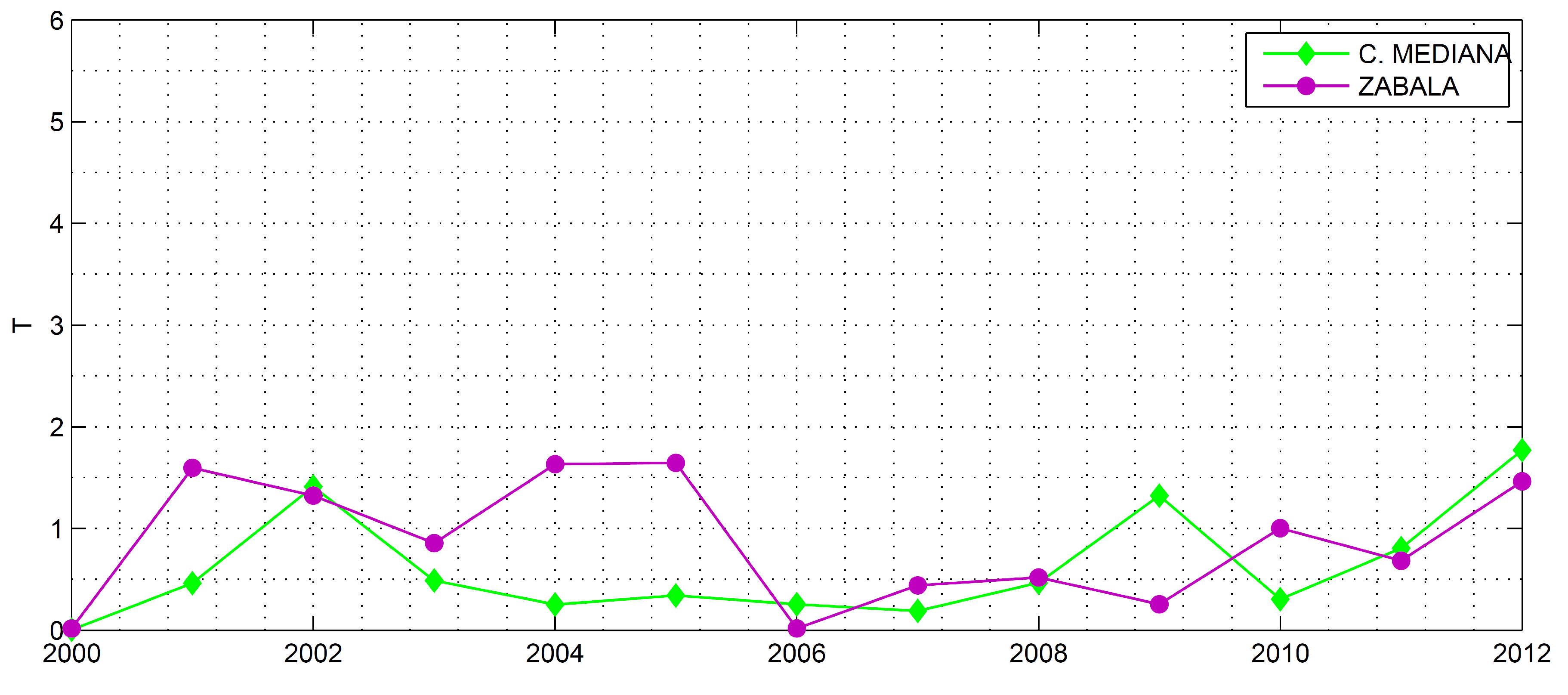
In order to check if the QAQC program really assured homogeneity [52] of time series and really minimized the effects of changes of instrument and/or changes in the sitting of specific instruments, an Alexandersson test [53] has been performed to Zabala and Cabeza Mediana temperature data sets for the period 2000–2014. A reference station belonging to the Spanish Meteorological Agency at a horizontal distance of 5 km was used for the test. The Puerto de Navacerrada (1893 m.a.s.l.) observatory follows standardized observation methods [52] and it is included in the SYNOP program. Figure 4 shows the results obtained. The T value of this test on the annual mean temperature is below the critical value (6 for 13 points) so the time series at these two sites can be considered comparable. Temperature time series recorded at these two sites are homogeneous despite the frequent changes in sensors during the period 2000–2014.
From this experience, we think that there are some factors that might not be detectable using these kind of tests but could probably be affecting the uncertainty of temperature data. The following ones should be further investigated in the future:
- effect of down-up short wave radiation reflected from ground due to snow cover. Radiation shields are designed for an up-down direction of direct radiation
- effect of raised ground level due to snow height in winter
- effect of evaporation of water drops condensed over the temperature sensor
One aspect that has shown to be useful for data validation is the relationship between values observed simultaneously at different sites (spatial coherency tests) and the local lapse rate. Figure 5 shows the mean hourly temperature for every site and season and for the common period. Considering the difference between mean maximum and minimum temperature as daily temperature amplitude, this figure shows how the temperature amplitude decreases with elevation. This decoupling led to temperature inversion episodes, which normally occurred during the first hours of the day. Differences between the maximum temperature at higher sites (Zabala, 2070 m.a.s.l.) and lower sites (Alameda, 1102 m.a.s.l.) were around 10 °C, a value very close to the dry adiabatic lapse rate. In winter this value was around 7 °C km, which is closer to the moist adiabatic lapse rate. The availability of long term sub-daily data for different altitudes will allow researchers in the future to go deeper into the analysis of the thermodynamic phenomena of this region.
Figure 6 shows the correlation between the hourly air temperatures for all the sites and for their common period. As expected, the correlation is high since the sites are relatively close to each other. Higher correlations are found among the higher altitude sites (Zabala, Cotos and Cabeza Mediana) and the valley bottom sites (Ontalva and Alameda).
3.3. Wind Observations
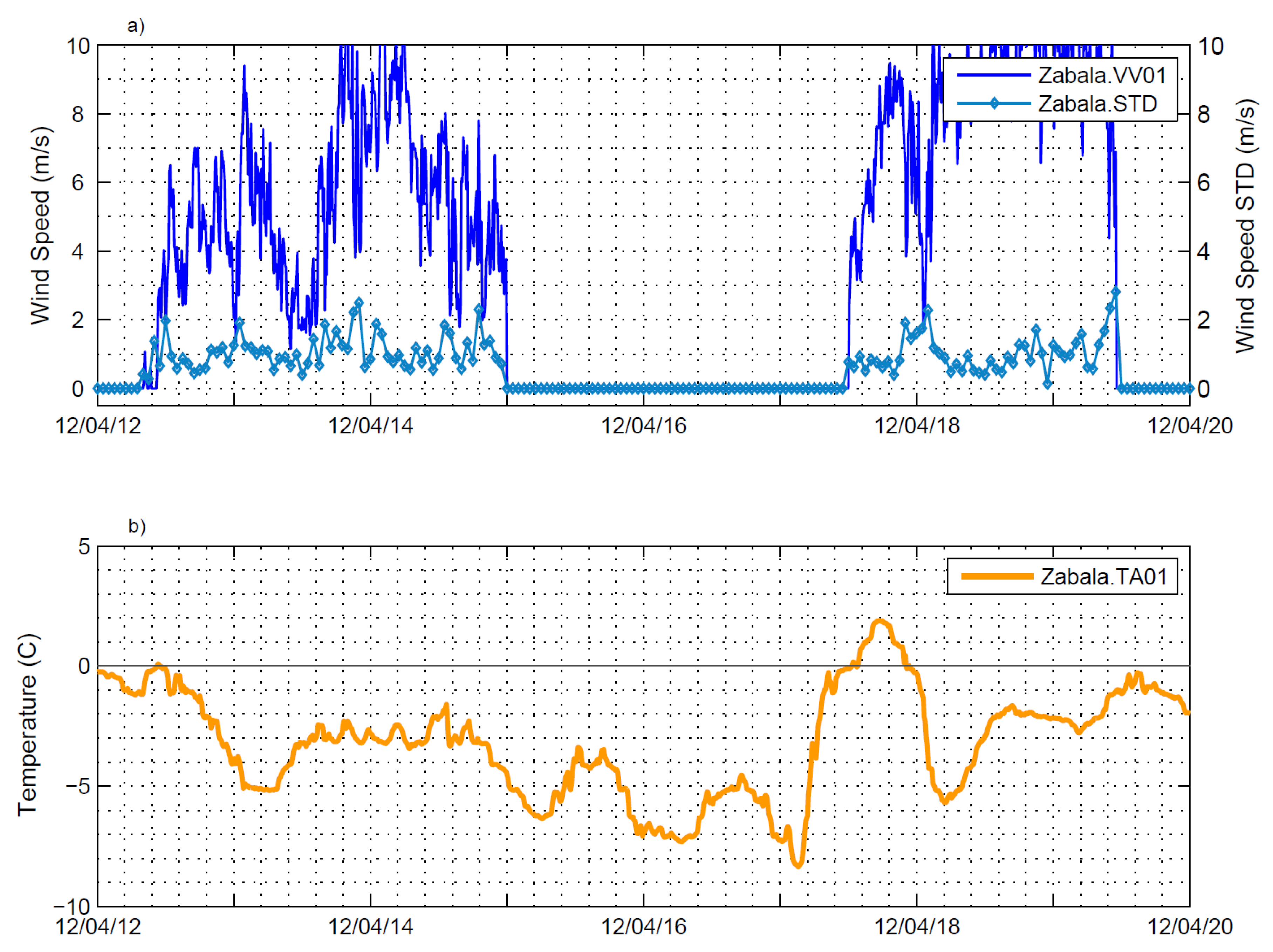
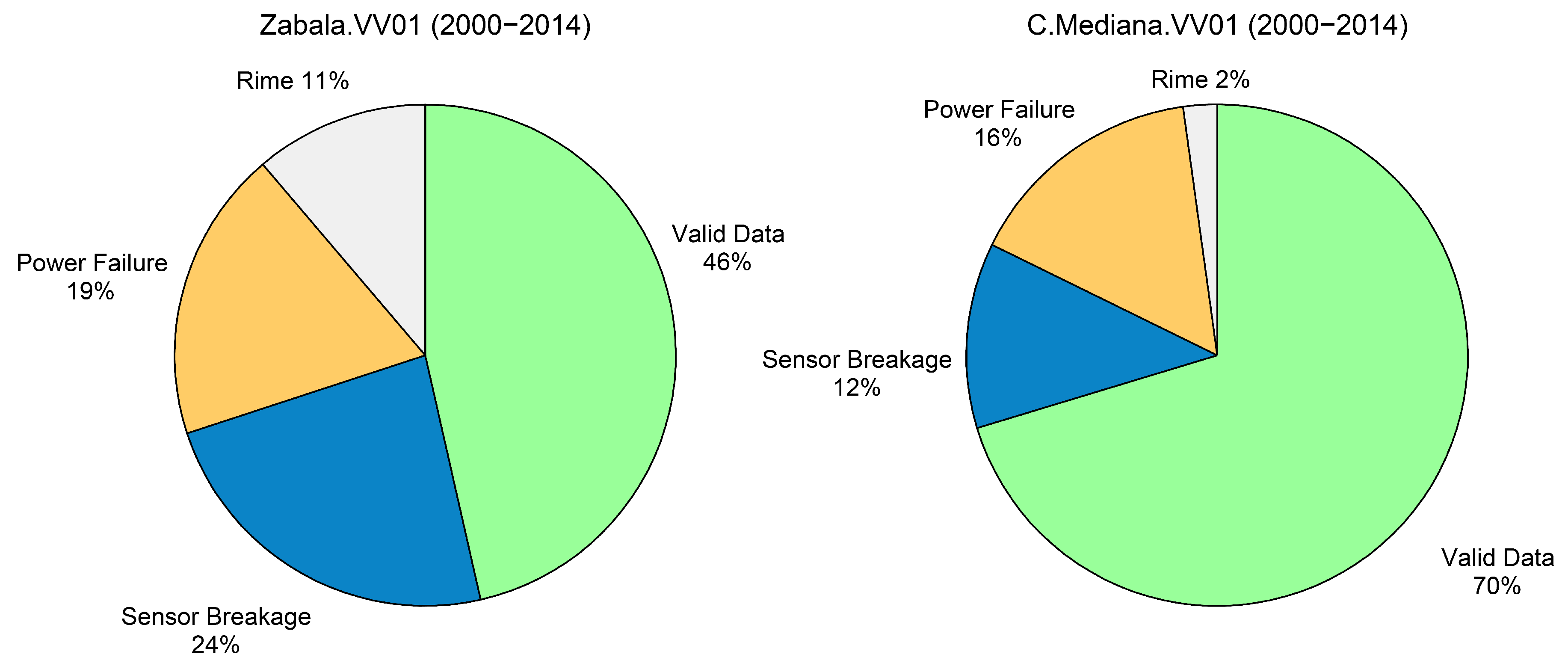
For wind speed and wind direction, mechanically driven sensors were chosen. In the past years, cup anemometers and wind vanes have been replaced with four blade helical propeller wind and direction sensors, which have shown to be more reliable and robust. Both kinds of sensors are susceptible to be frequently blocked and broken by rime together with high winds [64,65]. Figure 7a shows the wind speed measured at Zabala during some days in the winter along with the standard deviation in the same period. This is just an example of how rime affects anemometer observations. Super-cooled water freezes immediately when touching the anemometer, which finally loses its mobility after a certain time. This process occurs under freezing conditions and can last for some days (Figure 7b). When the temperature rises, ice melts and very often the anemometer becomes functional again. An asymmetrical melting process on the rotor of the anemometer can often cause it to break and lose functionality. Since this is a winter phenomenon, the need to replace sensors caused a considerable increase in data gaps due to delays waiting for safe and favorable conditions for the maintenance crew. Figure 8 shows the completeness of wind data for some sites at different elevations and for all seasons. The number of wind measurements taken under freezing conditions is also shown. This graph shows the strong relationship between both variables and how higher elevation sites are more susceptible to this kind of phenomena. Figure 9 reinforces this elevation dependency and shows the percentage of valid data and data gaps due to the general failure of the powering system, the effect of rime and sensor breakage. The difficulty in obtaining reliable data coverage in winter at high elevation sites without heated sensors seems clear.
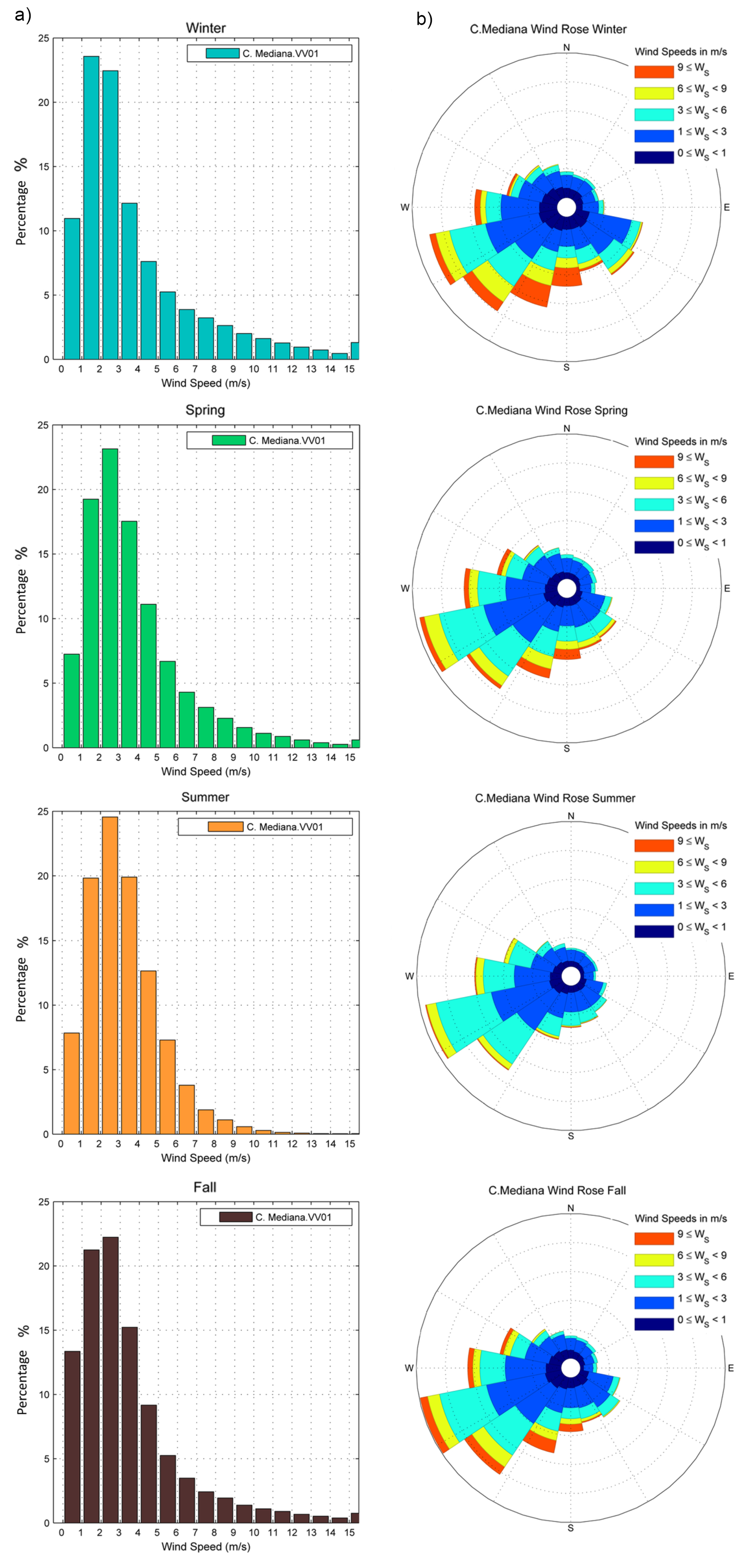
Besides the complexity of measuring wind under these conditions, and taking into account that the loss of data is causing a bias that would need further correction, a first assessment of wind at this area can be performed in the future by using the Cabeza Mediana site, which showed 70% of completeness for more than a decade. For illustration purposes the seasonal wind distribution has been calculated (Figure 10a) and the wind roses for this excellent wind monitoring site (Figure 10b).
3.4. Precipitation Observations
Regarding precipitation, this variable has shown to be extremely difficult to measure in these mountains, using tipping buckets. In the absence of wind, rain gauges perform fairly well since precipitation falls down vertically and is collected efficiently. Nevertheless, in real field conditions the catching process is less efficient and depends on other factors, like wind speed and precipitation rate. Even neglecting other sources of errors, only the influence of wind at the upper part of the rain gauge can be responsible for more than 15% losses in the case of rain and for 30% of snow, depending on wind speed and precipitation rate [66,67,68,69,70,71]. Therefore, it is generally accepted that rain gauges tend to underestimate values no matter what the measuring principle is. This effect is even more pronounced if wind shields are not used. In past years, there has been some relevant investigations regarding the methods of measurement that will be able to achieve a lower uncertainty for snow precipitation and mountain environments like the WMO SPICE project [72,73,74] and also newer methods to decrease uncertainty of gridded mountain precipitation data sets [75].
In addition to the loss of precipitation due to the aerodynamic effect of wind, the non-heated rain gauges used at RMPNP are normally blocked by snow during many winter, fall and spring days. When temperatures rise, the blocking snow at the funnel melts and spurious precipitation is recorded at the tipping-bucket under clear sky. This double effect of erroneous precipitation measurement is shown in Figure 11a. Here manual observations made at Cotos using a Hellman manual rain gauge is represented along with the automatic measurements. During the 27th and 28th of October snow precipitation was observed at the manual rain gauge, but nothing was detected by the tipping bucket rain gauge, which was collapsed by the snow. On the 2nd of March, the sky was clear as shown by the radiation sensor, and temperature rose above zero degrees (Figure 11b). Snow started to melt during the central hours of the day giving precipitation at a very constant and not very natural rate (Figure 11b). This process was confirmed by the snow depth sensor installed at the same site (Figure 11a). During this particular snow storm, 18 mm of snow fell in one day and 14 mm the following day, according to the manual rain gauge, but non-heated automatic rain gauge registered zero precipitation during the storm and a total of 3 mm in two days with a 48 hours phase error. Fortunately, this process was repeated with a similar pattern, so some algorithms were programmed to detect them.
At Guadarrama, most of the total precipitation that falls in winter, spring and fall is snow [14], so this is something that will need special attention for future network improvements.
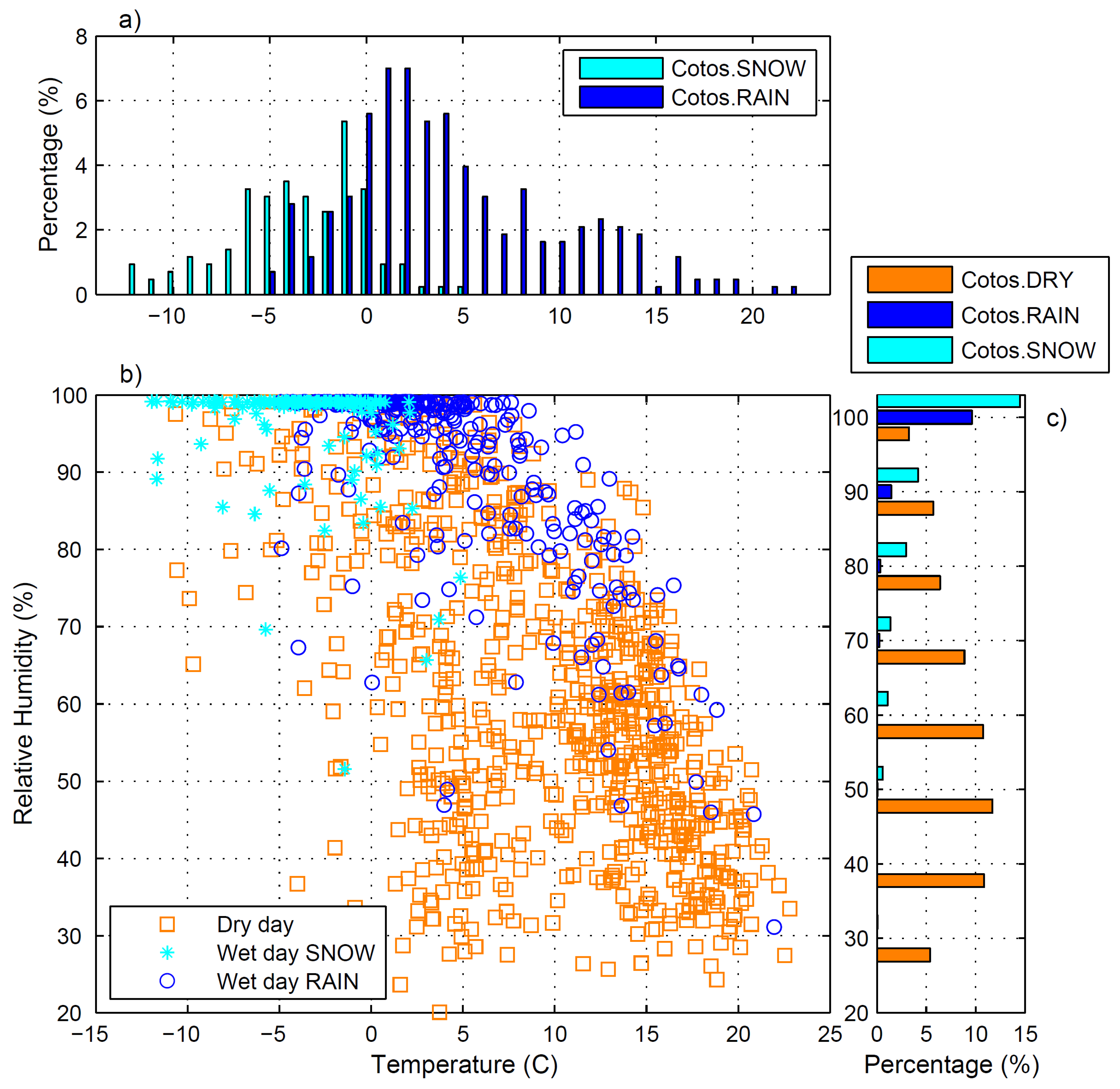
Figure 12b shows a scatter plot of days with precipitation below 1 mm (orange), days with snow precipitation higher than 1 mm (light blue) and days with rain precipitation higher than 1 mm (dark blue) against mean daily relative humidity and mean air temperature observed at Cotos. Precipitation was measured using a manual rain gauge. It seems clear how precipitation occurs more frequently with mean daily relative humidity values higher than 80%. This graph has been used as a three phase diagram with curves that have been used for the validation of precipitation data like the detection of false precipitation events or the malfunction of the tipping bucket. Refinements of this algorithm are expected to be done in the future discriminating between seasons and hours of the day, since relative humidity follows a clear daily cycle.
Going through an individual inspection of days with precipitation events with low mean relative humidity, it was found that some of them were errors on the manual collection, or precipitation that occurred on the limit of the collection period. Most of them could be related with convective storm activity. The episodes were characterized by a sudden and isolated increase of relative humidity lasting only a few hours.
These repeated patterns made it possible to use relative humidity as a good variable for internal coherency checks for precipitation.
Figure 12a also shows how snow, as expected, occurs mainly under freezing conditions, but again some exceptions were found. Obviously, this issue deserves deeper investigation.
In order to establish if the effect of precipitation underestimation of non-heated tipping bucket rain gauges is also affecting the rest of the rain gauges, the mean zero isotherm was calculated using hourly temperature and elevation of the sites. A linear adjustment of this data pairs gave an hourly lapse rate that was used to find the height for temperatures equal to 0 °C. Figure 13 shows the median, the 75th percentile and the 25th percentile of the zero isotherm elevations for winter months. This figure shows how during winter, as well as in parts of fall and spring, most of the sites (except Ontalva and Alameda) had, on average, freezing temperatures. It is then expected that the underestimation of precipitation is potentially occurring at all these sites. The precipitation observations for the winter period should be used with certain precaution.
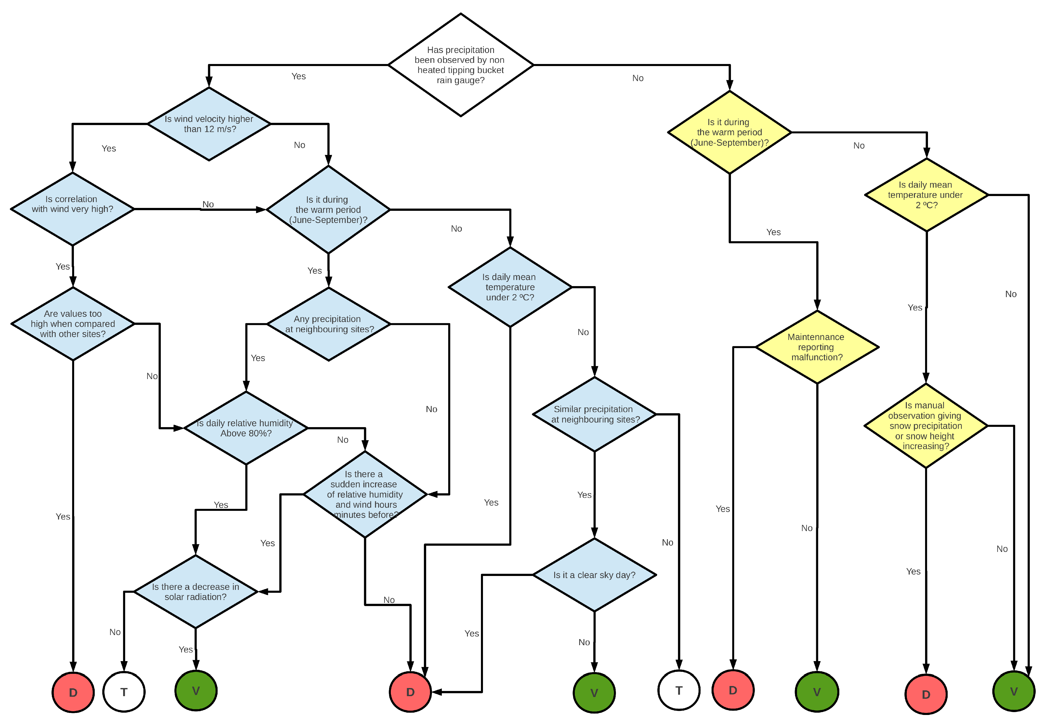
As a result of the experience throughout all these years, certain rules of thumb have been developed for the validation of precipitation. These rules are summarized in Figure 14 and should be taken as guidelines, since real cases at times are much more complex. This simple climographs indicate relevant differences among the different stations, and reinforce the need for a more detailed and a specific study, once the observational database is shown to be valid and robust.
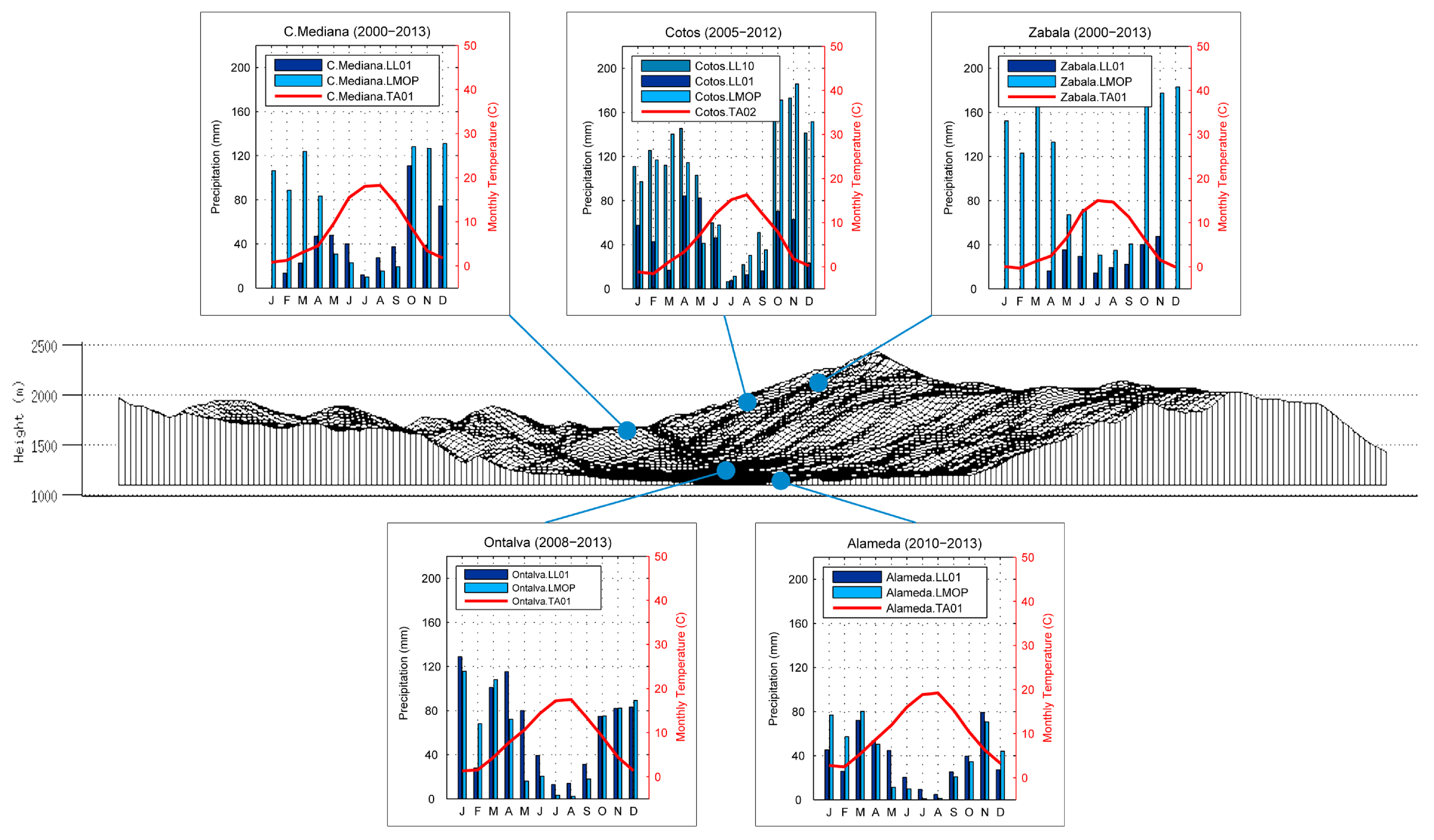
Automatic precipitation observations using non-heated tipping-bucket rain gauges are shown not to be valid for a complete, year-long assessment of precipitation at Guadarrama. In some cases, like convective episodes and under non-freezing conditions, manual and automatic measurements are comparable. Future users of this database might have to use other techniques, like modeling, for completing the observations. In order to give an estimation of the potential use of models for completing these data sets and also to give an order of magnitude of the missed precipitation, Figure 15 shows the results of a Linear Orographic Model [76] applied to this region [48]. This Figure shows an estimation of the climographs for each site and for each available period. Comparisons between sites should be made with precaution.
4. Conclusions
Fifteen years of operation of a mountain network like RMPNP enables us to extract some lessons that might be useful to the mountain observation community and users of the database which are summarized as follows:
- RMPNP evolved considerably from 1999, when the first station was installed, to 2014. The overall performance of the network has been improved in the last decade thanks to an optimization of the power consumption, application of a sustainable quality assurance program and the use of a reliable telecommunication system for operational alarms.
- Apart from the frequent sensor replacements, the logging system and changes made in data processing methods during this long operation period, the observations of air temperature at RMPNP have shown to be complete and homogeneous, hence they are valid for future climate analysis.
- Factors affecting data completion and reliability are common to other automatic networks, but here some negative factors gain prominence with increasing height like: icing, low solar power, difficulties for maintenance and breakage.
- A two phase validation based first on automatic checks when data is received for fast detection of errors and a second delayed phase which can be iteratively performed when new information is available, has shown to be efficient.
- Five automatic weather stations ranging from 1104 m.a.s.l. to 2079 m.a.s.l. of altitude but in a small territory of 40 km have been enough to show the complexity of the weather phenomena in the area, which should be further investigated.
- Temperature records in the area show a typical alpine behavior: decreasing temperatures with height with some inversion episodes during the first morning hours and a marked decreasing diurnal temperature amplitude. Monthly means have been calculated for every site, but a deeper analysis should be done in the future. For statistically representative trend analyses, longer records will be necessary so this should be done in the future if homogeneity of the series is kept.
- Regarding wind speed and direction, wind roses for the whole period have been calculated for the less locally influenced site. The prevailing wind direction is SW for all seasons. This is coherent with the prevailing synoptic wind directions, but also an orographic influence is expected since valley axis also runs in this direction. This issue should be investigated in the future.
- The horizontal axes four blade helical propeller wind anemometer and wind vane have shown to be more robust and less rime influenced than other non-heated mechanical alternatives. Power failure, sensor breakage and icing are the main sources of wind data loss. Icing is only responsible of 11% of the data loss at one of the higher sites.
- As expected, non-heated tipping bucket rain gauges have shown to perform fairly well only during spring, summer and fall if ambient temperature is above 5 °C, but they require a lot of effort for data validation.
- Manual observations of precipitation performed at one site in parallel with an automatic weather station have resulted in being crucial for assessing precipitation in the area. It has also helped to develop algorithms for data validation.
- Snow height measurement has shown to be a good estimator of snow precipitation when rain gauges are not operative, but further analysis will be necessary to convert height variations into equivalent precipitated water.
- From this experience and the available literature, we conclude that a basic but reliable automatic weather station at a very remote location only powered by the sun should consist of:
- -
- Precipitation: gravimetric measurement method for precipitation with very wide inlets (no funnels), with wind shields, using antifreeze during the winter and installed in a very solid mast above expected snow pack.
- -
- Temperature/Humidity: Low power aspirated radiation shields with smart management of the aspirated process in order to minimize power consumption. Redundant measurements of temperature at different angles should help to diminish and investigate the effect of rime and prevent data loss.
- -
- Wind: ultrasonic rugged sensors with a smart management of heating for lower consumption, if possible; not necessarily installed at the standard 10 m height since this jeopardizes the structural integrity and makes sensor substitution and maintenance much more complex. Sensor height will change with snow pack and should be taken into account.
- -
- Solar radiation: Sensors with a smart heating, low power algorithm should be found or developed. Investigation into minimum heating activation and detection of total or partial sensor malfunction due to ice and snow should be done in the future, perhaps by using cameras.
- -
- Ground temperature: Reliable soil temperature sensors at different depths are easy to perform and can be valid for data validation and gap filling.
- -
- Snow height: Ultrasonic sensors, which are crucial for correcting and validating many of the variables measured at this sites.
Acknowledgments
This network would have never existed without the funding and support from the Peñalara Natural Park and, specifically, the Park Director: Juan Vielva Juez. The intensive field work has been also possible through all these years thanks to the extraordinary help of the Park staff, the “A Team” for logistics and wise advice and “Cuerpo de Vigilantes” who performed manual observations and did a great job taking care of the installations throughout all these years. We would thank Carlos Yagüe Anguis for his wise suggestions and encouragement. Also, we would like to thank the reviewers for their insightful and constructive comments who surely helped this manuscript to be richer and more concise. We finally want to thank Dean Custer for his in-depth, accurated and exhaustive help with the correct writing of this manuscript.
Author Contributions
Luis Durán conceived, designed, installed and maintained this network from its beginnings in 1998 acquiring some know-how in the process thanks to some hits but more misses. Irene Rodríguez joined the project in recent years, giving a new impulse and working on the analysis and final databases. Enrique Sánchez has coordinated and supervised the manuscript structure and gave the necessary encouragement and support for this work to see the light eventually.
Conflicts of Interest
The authors declare no conflict of interest.
Abbreviations
The following abbreviations are used in this manuscript:
| AEMET | Agencia Estatal de MEteorología (Spanish Meteorological Agency) |
| ASCII | American Standard Code for Information Interchange |
| GPRS | General Packet Radio Service |
| GSM | Global System for Mobile communications |
| QAQC | Quality Assurance and control |
| RMPNP | Red Meteorológica del Parque Natural de Peñalara |
References
- Auer, I.; Böhm, R.; Jurkovic, A.; Lipa, W.; Orlik, A.; Potzmann, R.; Schoner, W.; Ungersbock, M.; Matulla, C.; Briffa, K.; et al. HISTALP—historical instrumental climatological surface time series of the Greater Alpine Region. Int. J. Climatol. 2007, 27, 17–46. [Google Scholar] [CrossRef]
- Hiebl, J.; Auer, I.; Böhm, R.; Schöner, W.; Maugeri, M.; Lentini, G.; Spinoni, J.; Brunetti, M.; Nanni, T.; Tadic, M.; et al. A high-resolution 1961–1990 monthly temperature climatology for the greater Alpine region. Meteorol. Z. 2009, 18, 507–530. [Google Scholar] [CrossRef]
- Barry, R.G. Changes in mountain climate and glacio-hydrological responses. Mt. Res. Dev. 1990, 10, 161–170. [Google Scholar] [CrossRef]
- Diaz, H.F.; Bradley, R.S. Temperature variations during the last century at high elevation sites. In Climatic Change at High Elevation Sites; Springer: Dordrecht, The Netherlands, 1997; pp. 21–47. [Google Scholar]
- Hauer, F.R.; Baron, J.S.; Campbell, D.H.; Fausch, K.D.; Hostetler, S.W.; Leavesley, G.H.; Leavitt, P.R.; McKnight, D.M.; Stanford, J.A. Assessment of climate change and freshwater ecosystems of the Rocky Mountains, USA and Canada. Hydrol. Process. 1997, 11, 903–924. [Google Scholar] [CrossRef]
- Jungo, P.; Beniston, M. Changes in the anomalies of extreme temperature anomalies in the 20th century at Swiss climatological stations located at different latitudes and altitudes. Theor. Appl. Climatol. 2001, 69, 1–12. [Google Scholar] [CrossRef]
- Bosch, J.; Martínez-Solano, I. Chytrid fungus infection related to unusual mortalities of Salamandra salamandra and Bufo bufo in the Penalara Natural Park, Spain. Oryx 2006, 40, 84–89. [Google Scholar] [CrossRef]
- Anderson, B.; Akçakaya, H.; Araújo, M.; Fordham, D.; Martinez-Meyer, E.; Thuiller, W.; Brook, B. Dynamics of range margins for metapopulations under climate change. Proc. R. Soc. Lond. B 2009, 276, 1415–1420. [Google Scholar] [CrossRef] [PubMed]
- Lurgi, M.; López, B.C.; Montoya, J.M. Climate change impacts on body size and food web structure on mountain ecosystems. Philos. Trans. R. Soc. Lond. B 2012, 367, 3050–3057. [Google Scholar] [CrossRef] [PubMed] [Green Version]
- Leppi, J.C.; DeLuca, T.H.; Harrar, S.W.; Running, S.W. Impacts of climate change on August stream discharge in the Central-Rocky Mountains. Clim. Chang. 2012, 112, 997–1014. [Google Scholar] [CrossRef]
- Fuhrer, J.; Smith, P.; Gobiet, A. Implications of climate change scenarios for agriculture in alpine regions—A case study in the Swiss Rhone catchment. Sci. Total Environ. 2014, 493, 1232–1241. [Google Scholar] [CrossRef] [PubMed]
- Buytaert, W.; Celleri, R.; Willems, P.; De Bievre, B.; Wyseure, G. Spatial and temporal rainfall variability in mountainous areas: A case study from the south Ecuadorian Andes. J. Hydrol. 2006, 329, 413–421. [Google Scholar] [CrossRef] [Green Version]
- De Pedraza-Gilsanz, J. Peñalara: Un paradigma para la conservación de las montañas? In Actas de los Segundas Jornadas Científicas del Parque Natural de Peñalara y Valle del Paular. Consejería de Medio Ambiente; Comunidad de Madrid: Madrid, Spain, 2000; pp. 9–18. [Google Scholar]
- Durán, L.; Sánchez, E.; Yagüe, C. Climatology of precipitation over the Iberian Central System mountain range. Int. J. Climatol. 2013, 33, 2260–2273. [Google Scholar] [CrossRef]
- Durán, L.; Rodríguez-Fonseca, B.; Yagüe, C.; Sánchez, E. Water vapour flux patterns and precipitation at Sierra de Guadarrama mountain range (Spain). Int. J. Climatol. 2015, 35, 1593–1610. [Google Scholar] [CrossRef]
- Palacios, D.; Sánchez-Colomer, M.G. The influence of geomorphologic heritage on present nival erosion: Peñalara, Spain. Geogr. Ann. Ser. A 1997, 79, 25–40. [Google Scholar] [CrossRef]
- Palacios, D.; Andrés, N. Morfodinámica supraforestal actual en la Sierra de Guadarrama y su relación con la cubierta nival: El caso de Dos Hermanas-Peñalara. In Procesos y Formas Periglaciares en la Montaña Mediterránea; Instituto de Estudios Turolenses: Teruel, Spain, 2000; pp. 235–264. [Google Scholar]
- Palacios, D.; de Andrés, N.; Luengo, E. Distribution and effectiveness of nivation in Mediterranean mountains: Peñalara (Spain). Geomorphology 2003, 54, 157–178. [Google Scholar] [CrossRef]
- Palacios, D.; de Andrés, N.; de Marcos, J.; Vázquez-Selem, L. Glacial landforms and their paleoclimatic significance in Sierra de Guadarrama, Central Iberian Peninsula. Geomorphology 2012, 139, 67–78. [Google Scholar] [CrossRef]
- Álvarez, R.; Sierra, F. Paisajes glaciares del macizo de Peñalara. In Biólogos: Revista del Colegio Oficial de Biólogos de la Comunidad de Madrid; Colegio Oficial de Biologos de la Comunidad de Madrid: Madrid, Spain, 2011; Volume 3, pp. 16–19. [Google Scholar]
- Granados, I.; Toro, M. Limnología en el Parque Natural de Peñalara: Nuevas aportaciones y perspectivas de futuro. In Actas de los Segundas Jornadas Científicas del Parque Natural de Peñalara y Valle del Paular. Consejería de Medio Ambiente; Comunidad de Madrid: Madrid, Spain, 2000; pp. 55–72. [Google Scholar]
- Granados, I.; Toro, M.; Rúbio-Romero, A. Laguna Grande de Peñalara: 10 años de Seguimiento Limnológico; Comunidad de Madrid: Madrid, Spain, 2006. [Google Scholar]
- Granados, I. ¿Cómo cambiará la laguna Grande de Peñalara frente al cambio climático? In Actas de las Quintas Jornadas Científicas del Parque Natural de Peñalara y Valle del Paular. Consejería de Medio Ambiente; Comunidad de Madrid: Madrid, Spain, 2007; pp. 43–52. [Google Scholar]
- Montouto, O. La flora vascular rara, endémica y amenazada del Parque Natural de Peñalara y su entorno. Amenazas y necesidades de conservación en la Finca de los Cotos. In Actas de las Segundas Jornadas Científicas del Parque Natural de Peñalara y Valle del Paular. Consejería de Medio Ambiente; Comunidad de Madrid: Madrid, Spain, 2000; pp. 33–53. [Google Scholar]
- Horcajada, F. Genética de las poblaciones de corzo en el Parque Natural de Peñalara. Foresta 2011, 52, 368–371. [Google Scholar]
- Juez, J.V. El buitre negro en el Parque Natural de Peñalara. Foresta 2011, 52, 363–365. [Google Scholar]
- Ortoz-Santaliestra, M.E.; Fisher, M.C.; Fernández-Beaskoetxea, S.; Fernández-Benéitez, M.J.; Bosch, J. Ambient ultraviolet B radiation and prevalence of infection by Batrachochytrium dendrobatidis in two amphibian species. Conserv. Biol. 2011, 25, 975–982. [Google Scholar] [CrossRef] [PubMed]
- Pérez, J.B. Los anfibios de Peñalara vuelven al paraíso. Foresta 2011, 52, 366–367. [Google Scholar]
- Sancho, L.G. Vegetación Liquénica y Procesos Naturales de Colonización en el Macizo de Peñalara. In Actas de las Segundas Jornadas Científicas del Parque Natural de Peñalara y Valle del Paular. Consejería de Medio Ambiente; Comunidad de Madrid: Madrid, Spain, 2000; pp. 27–32. [Google Scholar]
- Sancho, L.G.; De la Torre, R.; Horneck, G.; Ascaso, C.; de los Rios, A.; Pintado, A.; Wierzchos, J.; Schuster, M. Lichens survive in space: Results from the 2005 LICHENS experiment. Astrobiology 2007, 7, 443–454. [Google Scholar] [CrossRef] [PubMed]
- Gómez González, C.; Ruiz Zapata, M.B.; García, G.; José, M.; López Saez, J.A.; Santisteban Navarro, J.I.; Mediavilla López, R.M.; Domínguez Castro, F.; Vera López, S. Evolución del paisaje vegetal durante los últimos 1.680 años BP en el Macizo de Peñalara (Sierra de Guadarrama, Madrid). Rev. Esp. Micropaleontol. 2009, 41, 75–89. [Google Scholar]
- Schwaiger, H.P.; Bird, D.N. Integration of albedo effects caused by land use change into the climate balance: Should we still account in greenhouse gas units? For. Ecol. Manag. 2010, 260, 278–286. [Google Scholar] [CrossRef]
- García-Romero, A.; Muñoz, J.; Andrés, N.; Palacios, D. Relationship between climate change and vegetation distribution in the Mediterranean mountains: Manzanares Head valley, Sierra De Guadarrama (Central Spain). Clim. Chang. 2010, 100, 645–666. [Google Scholar] [CrossRef]
- Gutiérrez-Girón, A.; Gavilán, R.G. Spatial patterns and interspecific relations analysis help to better understand species distribution patterns in a Mediterranean high mountain grassland. Plant Ecol. 2010, 210, 137–151. [Google Scholar] [CrossRef]
- Moreno, J.L.I. La flora protegida de Peñalara. Foresta 2011, 52, 350–354. [Google Scholar]
- Mera, A.G.d.; Perea, E.L.; Orellana, J.A.V. Taraxacum penyalarense (Asteraceae), a new species from the Central Mountains of Spain. In Annales Botanici Fennici; BioOne: Washington, DC, USA, 2012; Volume 49, pp. 91–94. [Google Scholar]
- García-Camacho, R.; Albert, M.J.; Escudero, A. Small-scale demographic compensation in a high-mountain endemic: The low edge stands still. Plant Ecol. Divers. 2012, 5, 37–44. [Google Scholar] [CrossRef]
- García-Fernández, A.; Iriondo, J.M.; Bartels, D.; Escudero, A. Response to artificial drying until drought-induced death in different elevation populations of a high-mountain plant. Plant Biol. 2013, 15, 93–100. [Google Scholar] [CrossRef] [PubMed]
- Amat, M.E.; Vargas, P.; Gómez, J.M. Effects of human activity on the distribution and abundance of an endangered Mediterranean high-mountain plant (Erysimum penyalarense). J. Nat. Conserv. 2013, 21, 262–271. [Google Scholar] [CrossRef]
- Ruiz-Labourdette, D.; Schmitz, M.F.; Pineda, F.D. Changes in tree species composition in Mediterranean mountains under climate change: Indicators for conservation planning. Ecol. Indic. 2013, 24, 310–323. [Google Scholar] [CrossRef]
- Durán, L. Description and preliminary results of a meteorological network for high altitudes. Geophys. Res. Abs. 2003, 5, 12466. [Google Scholar]
- Bosch, J.; Carrascal, L.M.; Duran, L.; Walker, S.; Fisher, M.C. Climate change and outbreaks of amphibian chytridiomycosis in a montane area of Central Spain. Proc. R. Soc. Lond. B 2007, 274, 253–260. [Google Scholar] [CrossRef]
- Ruiz Zapata, M.B.; Gómez González, C.; García, G.; José, M.; López Saez, J.A.; Santisteban Navarro, J.I.; Mediavilla López, R.M.; Domínguez Castro, F.; Vera López, S. Reconstrucción de las condiciones paleoambientales del depósito Pñ (Macizo de Peñalara, Sierra de Guadarrama. Madrid), durante los últimos 2.000 años, a partir del contenido en microfósiles no polínicos (NPPs). Geogaceta 2009, 46, 135–138. [Google Scholar]
- Granados, I. Se puede medir el cambio global en Peñalara? Foresta 2011, 52, 28–29. [Google Scholar]
- Ruiz-Labourdette, D.; Martínez, F.; Martín-López, B.; Montes, C.; Pineda, F.D. Equilibrium of vegetation and climate at the European rear edge. A reference for climate change planning in mountainous Mediterranean regions. Int. J. Biometeorol. 2011, 55, 285–301. [Google Scholar] [CrossRef] [PubMed]
- Genova Fuster, M.d.M. Extreme pointer years in tree-ring records of Central Spain as evidence of climatic events and the eruption of the Huaynaputina Volcano (Peru, 1600 AD). Clim. Past 2012, 8, 751–764. [Google Scholar] [CrossRef] [Green Version]
- Sánchez-López, G.; Hernández, A.; Pla-Rabes, S.; Toro, M.; Granados, I.; Sigrò, J.; Trigo, R.M.; Rubio-Inglés, M.; Camarero, L.; Valero-Garcés, B.; et al. The effects of the NAO on the ice phenology of Spanish alpine lakes. Clim. Chang. 2015, 130, 101–113. [Google Scholar] [CrossRef] [Green Version]
- Durán, L.; Barstad, I. Multi-Scale Evaluation of a Linear Model of Orographic Precipitation Over Sierra de Guadarrama (Iberian Central System). Int. J. Climatol. 2017. under review. [Google Scholar]
- Rath, V. GUMNET-A new subsurface observatory in the Guadarrama Mountains, Spain. In Proceedings of the EGU General Assembly 2012, Vienna, Austria, 22–27 April 2012; Volume 14, p. 6475. [Google Scholar]
- Frei, T. Designing meteorological networks for Switzerland according to user requirements. Meteorol. Appl. 2003, 10, 313–317. [Google Scholar] [CrossRef]
- Brock, F.V.; Richardson, S.J. Meteorological Measurement Systems; Oxford University Press: Oxford, UK, 2001. [Google Scholar]
- WMO. Guide to Meteorological Instruments and Methods of Observation; WMO-No. 8; World Meteorological Organisation: Geneva, Switzerland, 2008. [Google Scholar]
- Alexandersson, H. A homogeneity test applied to precipitation data. Int. J. Climatol. 1986, 6, 661–675. [Google Scholar] [CrossRef]
- Merlone, A.; Lopardo, G.; Sanna, F.; Bell, S.; Benyon, R.; Bergerud, R.; Bertiglia, F.; Bojkovski, J.; Böse, N.; Brunet, M.; et al. The MeteoMet project–metrology for meteorology: Challenges and results. Meteorol. Appl. 2015, 22, 820–829. [Google Scholar] [CrossRef]
- Salvati, M.; Brambilla, E. Data Quality Control Procedures in Alpine Metereological Services; Università di Trento. Dipartimento di ingegneria civile e ambientale: Trento, Italy, 2008. [Google Scholar]
- Momjian, B. PostgreSQL: Introduction and Concepts; Addison-Wesley: New York, NY, USA, 2001; Volume 192. [Google Scholar]
- Achour, M.; Betz, F.; Dovgal, A.; Lopes, N. PHP Manual. Available online: http://php.net/manual/en/index.php (assessed on 7 July 2017).
- Van Rossum, G.; Drake, F.L., Jr. Python Reference Manual; Centrum voor Wiskunde en Informatica: Amsterdam, The Netherlands, 1995. [Google Scholar]
- Woodruff, S.; Diaz, H.; Elms, J.; Worley, S. COADS Release 2 data and metadata enhancements for improvements of marine surface flux fields. Phys. Chem. Earth 1998, 23, 517–526. [Google Scholar] [CrossRef]
- Leroy, M.; Tammelin, B.; Hyvönen, R.; Rast, J.; Musa, M. Temperature and humidity measurements during icing conditions. In Proceedings of the WMO Technical Conference on Meteorological and Environmental Instruments and Methods of Observation, Bratislava, Slovak, 23–25 September 2002. [Google Scholar]
- Appenzeller, C.; Begert, M.; Zenklusen, E.; Scherrer, S.C. Monitoring climate at Jungfraujoch in the high Swiss Alpine region. Sci. Total Environ. 2008, 391, 262–268. [Google Scholar] [CrossRef] [PubMed]
- Heimo, A.; Cattin, R.; Calpini, B. Recommendations for meteorological measurements under icing conditions. In Proceedings of the IWAIS XIII, Andermatt, Switzerland, 8–11 September 2009. [Google Scholar]
- Thomas, C.K.; Smoot, A.R. An effective, economic, aspirated radiation shield for air temperature observations and its spatial gradients. J. Atmos. Oceani. Technol. 2013, 30, 526–537. [Google Scholar] [CrossRef]
- Makkonen, L.; Lehtonen, P.; Helle, L. Anemometry in icing conditions. J. Atmos. Ocean. Technol. 2001, 18, 1457–1469. [Google Scholar] [CrossRef]
- Fortin, G.; Perron, J.; Ilinca, A. Behaviour and modeling of cup anemometers under Icing conditions. In Proceedings of the IWAIS XI, Montréal, QC, Canada, 16 June 2005; p. 6. [Google Scholar]
- Groisman, P.Y.; Legates, D.R. The accuracy of United States precipitation data. Bull. Am. Meteorol. Soc. 1994, 75, 215–227. [Google Scholar] [CrossRef]
- Sevruk, B. Adjustment of tipping-bucket precipitation gauge measurements. Atmos. Res. 1996, 42, 237–246. [Google Scholar] [CrossRef]
- Goodison, B.; Louie, P.; Yang, D. The WMO Solid Precipitation Measurement Intercomparison; World Meteorological Organization: Geneva, Switzerland, 1997; pp. 65–70. [Google Scholar]
- Sieck, L.C.; Burges, S.J.; Steiner, M. Challenges in obtaining reliable measurements of point rainfall. Water Resour. Res. 2007, 43. [Google Scholar] [CrossRef]
- Paulat, M.; Frei, C.; Hagen, M.; Wernli, H. A gridded dataset of hourly precipitation in Germany: Its construction, climatology and application. Meteorol. Z. 2008, 17, 719–732. [Google Scholar] [CrossRef]
- Cheval, S.; Baciu, M.; Dumitrescu, A.; Breza, T.; Legates, D.R.; Chendeş, V. Climatologic adjustments to monthly precipitation in Romania. Int. J. Climatol. 2011, 31, 704–714. [Google Scholar] [CrossRef]
- Yang, D. Double fence intercomparison reference (DFIR) vs. bush gauge for “true” snowfall measurement. J. Hydrol. 2014, 509, 94–100. [Google Scholar] [CrossRef]
- Zhang, L.; Zhao, L.; Xie, C.; Liu, G.; Gao, L.; Xiao, Y.; Shi, J.; Qiao, Y. Intercomparison of solid precipitation derived from the weighting rain gauge and optical instruments in the interior Qinghai-Tibetan Plateau. Adva. Meteorol. 2015, 2015, 936724. [Google Scholar] [CrossRef]
- Kochendorfer, J.; Rasmussen, R.; Wolff, M.; Baker, B.; Hall, M.E.; Meyers, T.; Landolt, S.; Jachcik, A.; Isaksen, K.; Brækkan, R.; et al. The quantification and correction of wind-induced precipitation measurement errors. Hydrol. Earth Syst. Sci. 2017, 21, 1973–1989. [Google Scholar] [CrossRef]
- Neiman, P.J.; Ralph, F.M.; Wick, G.A.; Lundquist, J.D.; Dettinger, M.D. Meteorological characteristics and overland precipitation impacts of atmospheric rivers affecting the West Coast of North America based on eight years of SSM/I satellite observations. J. Hydrometeorol. 2008, 9, 22–47. [Google Scholar] [CrossRef]
- Smith, R.B.; Barstad, I. A linear theory of orographic precipitation. J. Atmos. Sci. 2004, 61, 1377–1391. [Google Scholar] [CrossRef]
Figure 1.
(a) Location of the Peñalara Natural Park Meteorological Network in Sierra de Guadarrama; (b) Location of the automatic monitoring stations.
Figure 1.
(a) Location of the Peñalara Natural Park Meteorological Network in Sierra de Guadarrama; (b) Location of the automatic monitoring stations.

Figure 2.
Flow chart of RMPNP data management and QAQC system.

Figure 3.
Time series of daily air temperature at the five sites from 2000 to 2014.
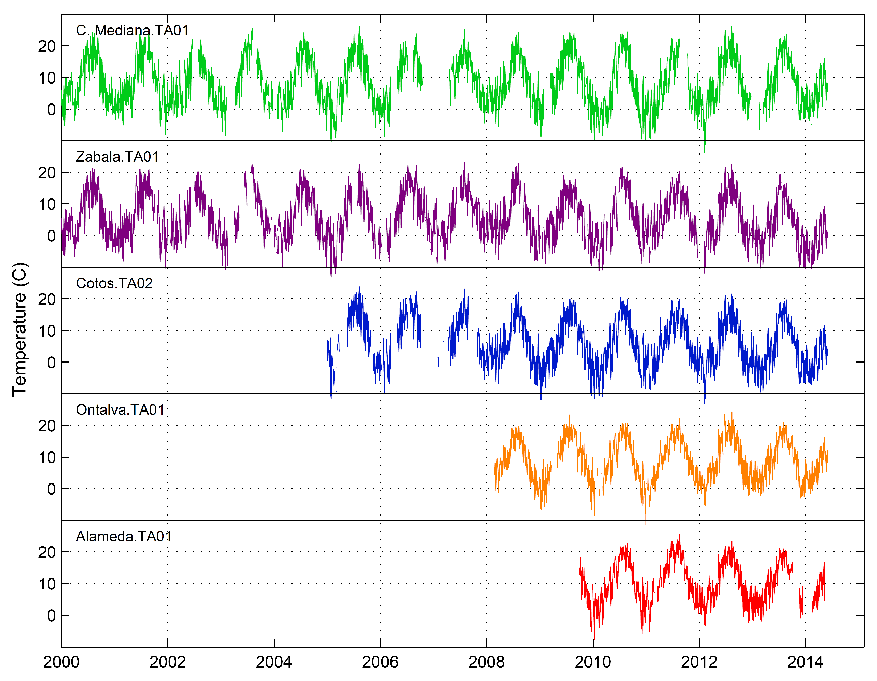
Figure 4.
Values of T of an Alexandersson test for annual mean temperature observed at Cabeza Mediana and Zabala using Puerto de Navacerrada AEMET (Agencia Estatal de MEteorología) observatory as a reference station. The critical T value for 5% confidence level and 14 samples is 6.
Figure 4.
Values of T of an Alexandersson test for annual mean temperature observed at Cabeza Mediana and Zabala using Puerto de Navacerrada AEMET (Agencia Estatal de MEteorología) observatory as a reference station. The critical T value for 5% confidence level and 14 samples is 6.

Figure 5.
Mean hourly temperature for every site and season. Differences between maximum and minimum temperatures represent the mean seasonal temperature amplitude.
Figure 5.
Mean hourly temperature for every site and season. Differences between maximum and minimum temperatures represent the mean seasonal temperature amplitude.
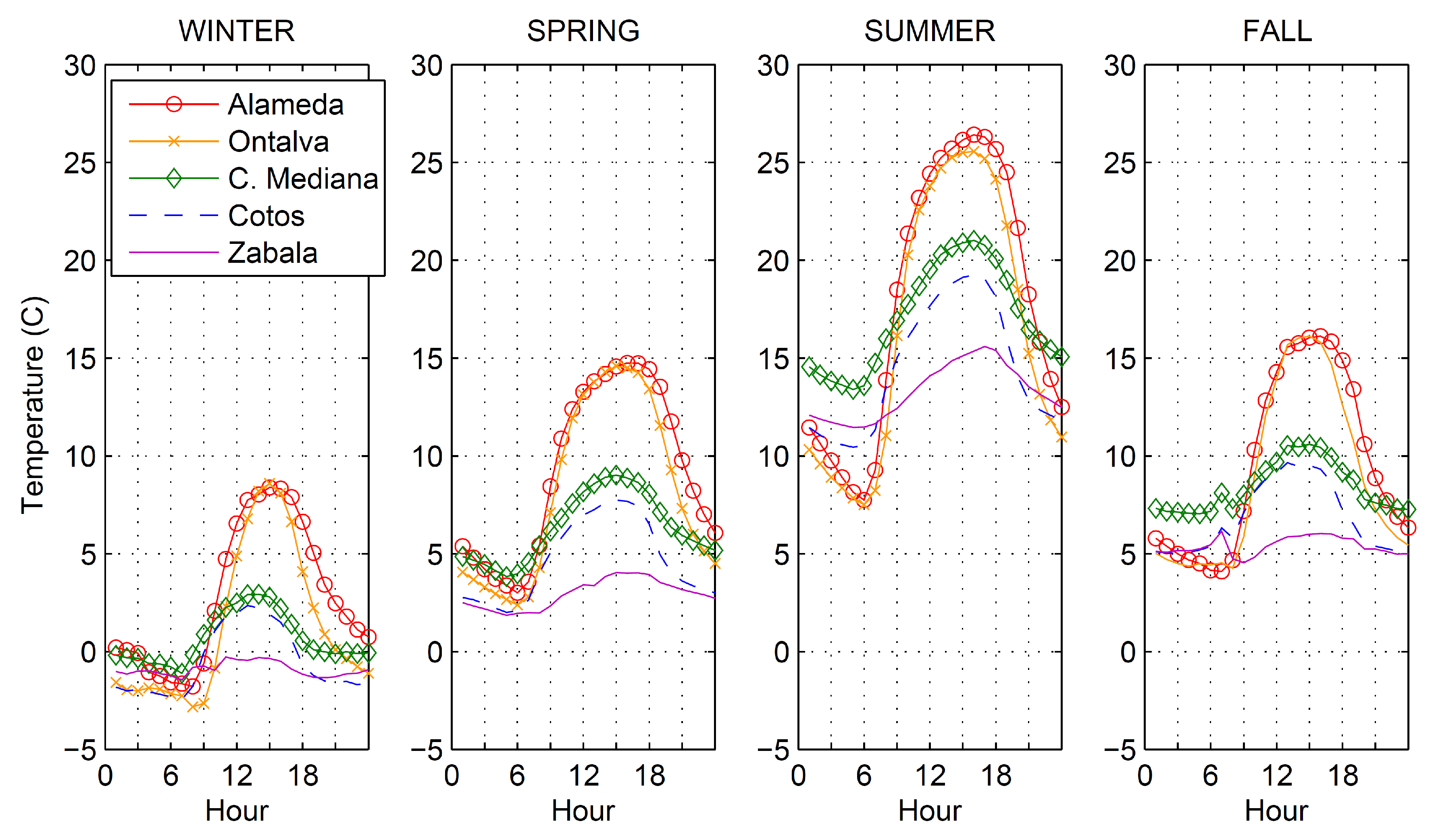
Figure 6.
Correlation coefficients of air temperature 10 min time series between all the sites of the network. Width of the lines is proportional to the Pearson correlation factor value.
Figure 6.
Correlation coefficients of air temperature 10 min time series between all the sites of the network. Width of the lines is proportional to the Pearson correlation factor value.
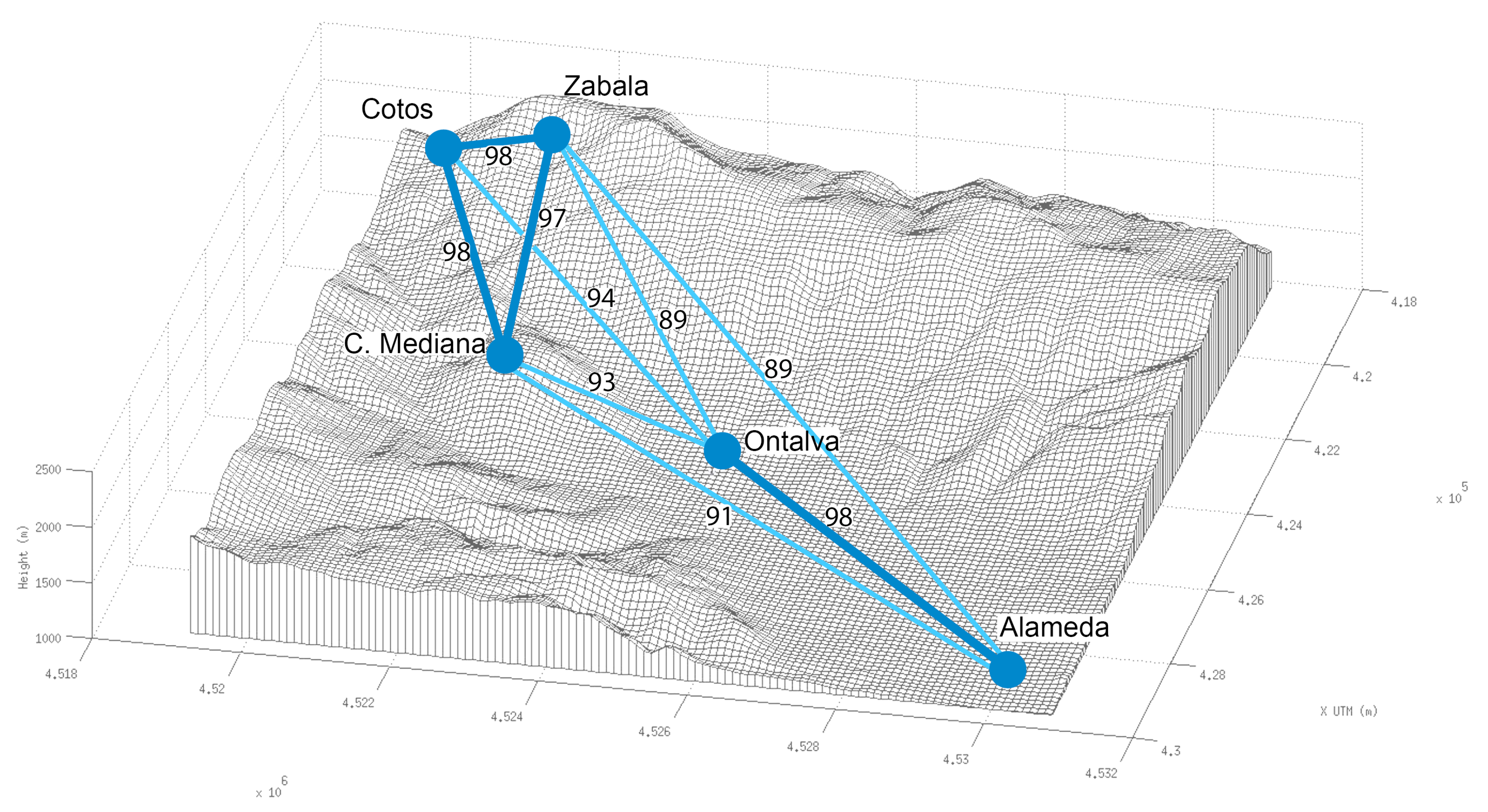
Figure 7.
(a) Wind speed (Zabala.VV01) and standard deviation of wind speed (Zabala.STD) at Zabala site during a period affected by freezing rime; (b) Air temperature (Zabala.TA01) at Zabala during the same period.
Figure 7.
(a) Wind speed (Zabala.VV01) and standard deviation of wind speed (Zabala.STD) at Zabala site during a period affected by freezing rime; (b) Air temperature (Zabala.TA01) at Zabala during the same period.

Figure 8.
Data completeness (blue) for three sites and percentage of wind speed measurements taken under freezing conditions (orange).
Figure 8.
Data completeness (blue) for three sites and percentage of wind speed measurements taken under freezing conditions (orange).
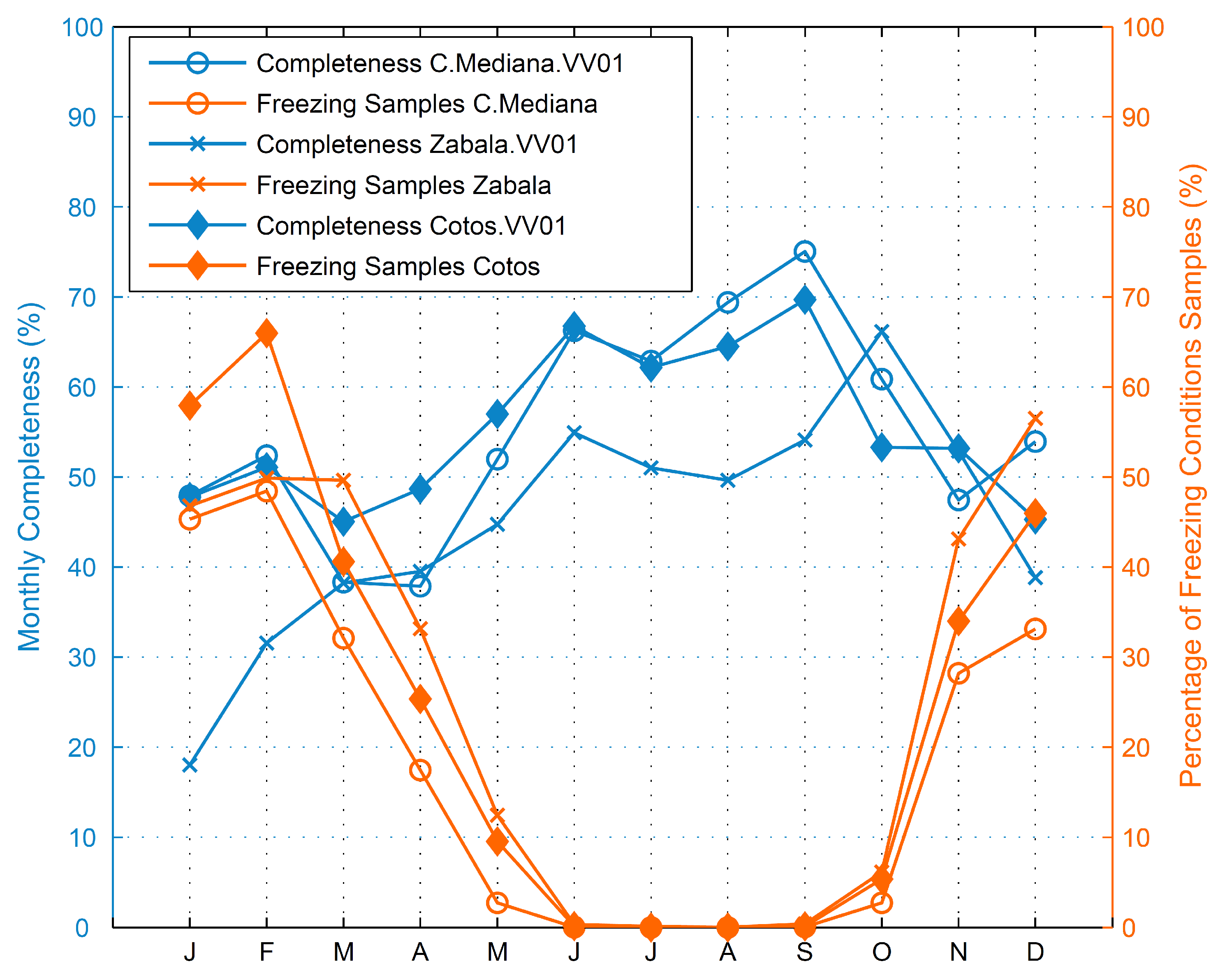
Figure 9.
Percentage of factors that lead to wind speed data loss (rime, power failure and sensor breakage) and total valid data at Zabala and Cabeza Mediana sites.
Figure 9.
Percentage of factors that lead to wind speed data loss (rime, power failure and sensor breakage) and total valid data at Zabala and Cabeza Mediana sites.

Figure 10.
(a) Seasonal wind speed distribution at Cabeza Mediana for the period 2000–2014; (b) Seasonal wind rose at Cabeza Mediana for the period 2000–2014.
Figure 10.
(a) Seasonal wind speed distribution at Cabeza Mediana for the period 2000–2014; (b) Seasonal wind rose at Cabeza Mediana for the period 2000–2014.

Figure 11.
(a) Precipitation observed using both a manual (Cotos.LL10) and a non-heated tipping bucket (Cotos.LL01) rain gauge, and the snow height in Cotos site for the same period; (b) Air temperature (Cotos.TA02) and solar radiation (Cotos.RT01) observed at Cotos site.
Figure 11.
(a) Precipitation observed using both a manual (Cotos.LL10) and a non-heated tipping bucket (Cotos.LL01) rain gauge, and the snow height in Cotos site for the same period; (b) Air temperature (Cotos.TA02) and solar radiation (Cotos.RT01) observed at Cotos site.
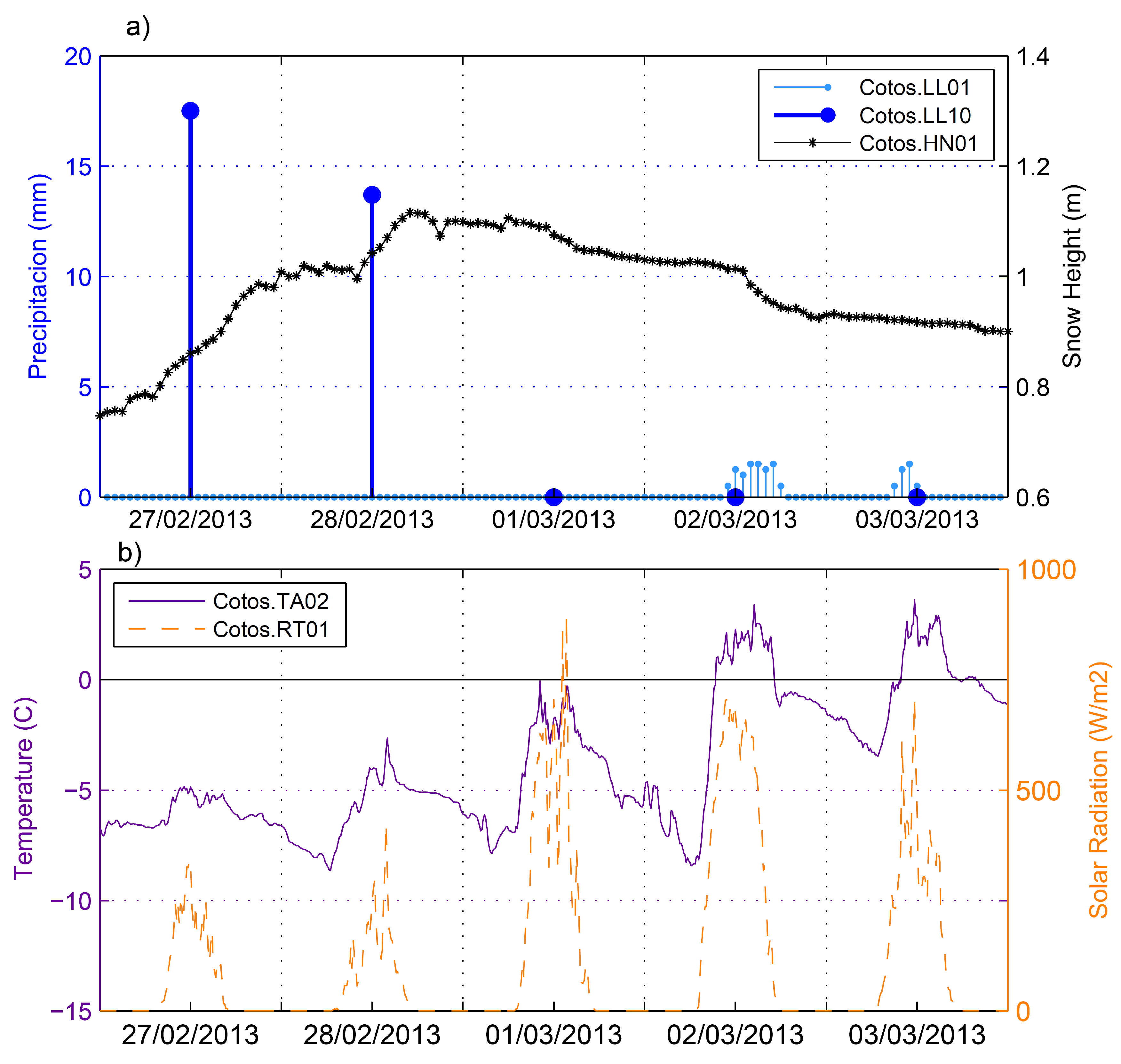
Figure 12.
(a) Bar plot of rain (Cotos.RAIN) and snow (Cotos.SNOW) observed using a manual rain gauge at Cotos for different values of daily mean air temperature; (b) Scatter plot of daily relative humidity against daily temperature for days with precipitation under 1 mm (squares), days with snow precipitation above than 1 mm (asterisks) and days with rain precipitation above 1 mm (circles) at Cotos; (c) Bar plot of percentage of days with precipitation under 1 mm (Cotos.DRY), days with snow precipitation (Cotos.SNOW) and days with rain precipitation (Cotos.RAIN) above 1 mm and mean daily relative humidity.

Figure 13.
Median, 75th percentile and 25th percentile of elevations of the zero isotherm for winter months calculated out of the temperatures observed at all sites.
Figure 13.
Median, 75th percentile and 25th percentile of elevations of the zero isotherm for winter months calculated out of the temperatures observed at all sites.

Figure 14.
Guidelines for precipitation validation. “V” means data with a high probability of being valid. “D” means data with a high probability of not being valid. “T” means data with an incoherent behavior with other variables (internal consistency) or other sites (spatial consistency) and which deserve further research elevations of the zero isotherm for winter months calculated out of the temperatures observed at all sites.

Figure 15.
Mean monthly temperature (TA01, TA02) and precipitation observed (LL01, LL10) and modeled (LMOP) at all sites.
Figure 15.
Mean monthly temperature (TA01, TA02) and precipitation observed (LL01, LL10) and modeled (LMOP) at all sites.

Table 1.
Annual average of data completeness of the stations based on availability of air temperature observations (Bold for completeness ≥75% and white for not fully operative). Collection method are Local that stands for in situ downloading of data, GSM for analog GSM data collection using modem and GPRS for GPRS TCP/IP protocol using dynamic IPs. Regarding Storage, ASCII stands for individual raw files from data logger, S.Sheet stands for spread sheets for every variable organized in years with individual validation code and SQL stands for PosgreSQL database storage.
| Year | Collection | Volume | Storage | Station | ||||
|---|---|---|---|---|---|---|---|---|
| Method | Data (bytes) | 001 | 002 | 003 | 004 | 005 | ||
| Ontalva | C. Mediana | Zabala | Cotos | Alameda | ||||
| 1999 | Local | 202039 | ASCII | 34 | 42 | |||
| 2000 | Local | 722874 | ASCII | 98 | 100 | |||
| 2001 | Local | 1015623 | ASCII | 96 | 94 | |||
| 2002 | Local | 1698549 | ASCII | 83 | 73 | |||
| 2003 | Local | 2198111 | ASCII | 63 | 61 | |||
| 2004 | Local | 2850198 | ASCII | 84 | 89 | |||
| 2005 | Local | 3613656 | S.Sheet | 91 | 85 | 96 | ||
| 2006 | GSM | 4219771 | S.Sheet | 55 | 58 | 51 | ||
| 2007 | GSM | 5375096 | S.Sheet | 66 | 80 | 56 | ||
| 2008 | GPRS | 7510050 | SQL | 84 | 92 | 90 | 96 | |
| 2009 | GPRS | 9911400 | SQL | 88 | 87 | 88 | 98 | 21 |
| 2010 | GPRS | 12634429 | SQL | 81 | 100 | 75 | 95 | 99 |
| 2011 | GPRS | 15261155 | SQL | 95 | 80 | 83 | 98 | 88 |
| 2012 | GPRS | 18022734 | SQL | 97 | 93 | 84 | 99 | 100 |
| 2013 | GPRS | 20629862 | SQL | 100 | 80 | 79 | 100 | 82 |
| 2014 | GPRS | 21966337 | SQL | 99 | 77 | 75 | 99 | 55 |
| Average | 92 | 80 | 79 | 89 | 75 | |||
Table 2.
Some comments on the completeness of the sites.
| Code | Name | Comments on Measurements Uncertainties |
|---|---|---|
| 001 | Ontalva | This station is located in the lower land of the valley. Land use is natural grass immersed into a pine forest in a sheltered clear. Wind observation is not very representative of the boundary layer wind due to obstacles, much higher than tower. The not heated rain gauge might under sample in winter due to snow blocking. Minimum temperatures are lower than expected due to this location is immersed in Valle de la Umbría, a north oriented valley within Lozoya Valley. Cold air drainage from higher elevations is also expected |
| 002 | Cabeza Mediana | Mountain site. Land use is natural pasture with some small trees. Nice location in the top of a flat and round ended hill in the middle of Valle del Lozoya. Promising representation of wind measurements. Not heated rain gauge is surely under sampling real precipitation in winter |
| 003 | Refugio Zabala | Very high mountain environmental conditions. Land use is mainly bare rock with snow cover during many months. Sensors are located in the top of small construction for security and impact reasons, so some impact is expected in wind and precipitation measurements. Good representation of temperature at 4 m but rime might be influencing temperature measurements in winter. Not heated rain gauge, so precipitation measurements are surely under sampled in winter |
| 004 | Cotos | High mountain site. Land use is natural pasture with tall pine trees at 100 m. Good representation but the site is located not in a very flat area. Local effects of catabatic cold air drainage from higher terrain is expected due to the slope. Not heated rain gauge, so precipitation measurements are surely under sampled |
| 005 | Alameda | Good representation of all measurements. Land use is natural grass. Even though rain gauge is not heated, under sampling might be less important due to less snow precipitation at this altitude, but needs to be taken into account in winter |
Table 3.
Description of the location and characteristics of the observing sites of Peñalara Meteorological Network. Instrumentation has changed since first installation but last one is included in this table
Table 3.
Description of the location and characteristics of the observing sites of Peñalara Meteorological Network. Instrumentation has changed since first installation but last one is included in this table
| Code | Name | Coordinates (City, Province) | UTM (m) Altitude (m.a.s.l.) | Starting Year | Variable Code | Magnitude (Units) | Sensor (2014) |
|---|---|---|---|---|---|---|---|
| 001 | Ontalva | 2008 | TA01 | Air temperature at 2 m (°C) | Vaisala HMP45 | ||
| 40°5220 N | X: 424736 | 2008 | HR01 | Relative humidity at 2 m (%) | Vaisala HMP45 | ||
| 3°531 W | Y: 4524980 | 2008 | LL01 | Liquid precipitation at 3 m (mm) | NovaLynx 260-2500 | ||
| (Rascafría, Madrid) | Z: 1190 | 2008 | VV01 | Wind velocity at 6 m (m/s) | NRG #40 | ||
| 2008 | DV01 | Wind direction at 6 m (°) | NRG | ||||
| 002 | 1999 | TA01 | Air temperature at 2 m (°C) | Vaisala HMP45 | |||
| 40°5013 N | X: 423450 | 1999 | HR01 | Relative humidity at 2 m (%) | Vaisala HMP45 | ||
| Cabeza | 3°5415 W | Y: 4521790 | 1999 | LL01 | Liquid precipitation at 3 m (mm) | NovaLynx 260-2500 | |
| Mediana | (Rascafría, Madrid) | Z: 1691 | 1999 | VV01 | Wind velocity at 6 m (m/s) | Young Wind Monitor | |
| 1999 | DV01 | Wind direction at 6 m (°) | Young Wind Monitor | ||||
| 2008 | PA01 | Atmospheric pressure at 1.75 m (hPa) | NovaLynx | ||||
| 003 | 1999 | TA01 | Air temperature at 2 m (°C) | Vaisala HMP45 | |||
| 1999 | HR01 | Relative humidity at 2 m (%) | Vaisala HMP45 | ||||
| Refugio | 40°5020 N | X: 419300 | 1999 | LL01 | Liquid precipitation at 4 m (mm) | Young wind monitor | |
| Zabala | 3°571 W | Y: 4521330 | 2008 | LL02 | Liquid precipitation at 4 m (mm) | Lambrecht | |
| (Rascafría, Madrid) | Z: 2079 | 1999 | VV01 | Wind velocity at 6 m (m/s) | Young Wind Monitor | ||
| 1999 | DV01 | Wind direction at 6 m (°) | Young Wind Monitor | ||||
| 2008 | PA01 | Atmospheric pressure at 1.75 m (hPa) | NovaLynx | ||||
| 004 | Cotos | 2008 | TA02 | Air temperature at 2 m (°C) | E+E Elektronic | ||
| 2005 | TA01 | Air temperature at 10 m (°C) | E+E Elektronic | ||||
| 40°4931 N | X: 418955 | 2008 | HR02 | Relative humidity at 2 m (%) | E+E Elektronic | ||
| 3°40 W | Y: 4519800 | 2005 | LL01 | Liquid precipitation at 1.5 m (mm) | NovaLynx | ||
| (Rascafría, Madrid) | Z: 1857 | 2005 | VV01 | Wind velocity at 10 m (°) | NGR #40 | ||
| 2005 | DV01 | Wind direction at 10 m (°) | NGR | ||||
| 2008 | HN01 | Snow height (m) | Judd Comunicatio | ||||
| 005 | Alameda | 40°5453 N | X: 428934 | 2009 | TA01 | Air temperature at 4 m (°C) | E+E Elektronic |
| 3°5039 W | Y: 4529640 | 2009 | HR01 | Relative humidity at 4 m (%) | E+E Elektronic | ||
| (Alameda, Madrid) | Z: 1102 | 2009 | LL01 | Liquid precipitation at 4 m (mm) | NovaLynx |
© 2017 by the authors. Licensee MDPI, Basel, Switzerland. This article is an open access article distributed under the terms and conditions of the Creative Commons Attribution (CC BY) license (http://creativecommons.org/licenses/by/4.0/).
Share and Cite
MDPI and ACS Style
Durán, L.; Rodríguez-Muñoz, I.; Sánchez, E. The Peñalara Mountain Meteorological Network (1999–2014): Description, Preliminary Results and Lessons Learned. Atmosphere 2017, 8, 203. https://doi.org/10.3390/atmos8100203
AMA Style
Durán L, Rodríguez-Muñoz I, Sánchez E. The Peñalara Mountain Meteorological Network (1999–2014): Description, Preliminary Results and Lessons Learned. Atmosphere. 2017; 8(10):203. https://doi.org/10.3390/atmos8100203
Chicago/Turabian StyleDurán, Luis, Irene Rodríguez-Muñoz, and Enrique Sánchez. 2017. "The Peñalara Mountain Meteorological Network (1999–2014): Description, Preliminary Results and Lessons Learned" Atmosphere 8, no. 10: 203. https://doi.org/10.3390/atmos8100203
Note that from the first issue of 2016, this journal uses article numbers instead of page numbers. See further details here.