The Air-Sea Nitrous Oxide Flux along Cruise Tracks to the Arctic Ocean and Southern Ocean


Key Laboratory of Global Change and Marine-Atmospheric Chemistry of the State Oceanographic Administration (SOA), Third Institute of Oceanography, Xiamen 361005, China
*
Authors to whom correspondence should be addressed.
Atmosphere 2017, 8(11), 216; https://doi.org/10.3390/atmos8110216
Submission received: 25 August 2017
/
Revised: 26 October 2017
/
Accepted: 26 October 2017
/
Published: 13 November 2017
(This article belongs to the Section Biosphere/Hydrosphere/Land–Atmosphere Interactions)
Abstract
:Nitrous oxide is a trace gas with two global environmental effects: it depletes stratospheric ozone and contributes to the greenhouse effect. Oceans are one of the most significant nitrous oxide sources; however, there are ocean areas whose contributions to the nitrous oxide budget are not yet well studied. The Southern Ocean and the Arctic Ocean feature strong winds and portions that are covered by sea ice. These intense environmental conditions and the remoteness of these regions hamper fieldwork; hence, very limited data are available on the distributions and the source and sink characteristics of nitrous oxide. Using data from the 4th Chinese National Arctic Research Expedition and the 27th Chinese National Antarctic Research Expedition, the first global-scale investigation of the surface water N2O distribution pattern, the factors influencing the N2O distribution and the air-sea N2O flux are discussed in this study. The results show that the tropical and subtropical regions (30° N–30° S) exhibit significant source characteristics, with a maximum air-sea flux of approximately 21.0 ± 3.9 μmol·m−2·d−1. The high air-sea flux may result from the coastal influences and high wind speeds in certain areas. The distribution patterns of N2O in the sub-polar regions (30° N–60° N, 30° S–60° S) transition from oversaturated to approximate equilibrium with the atmosphere, and the boundaries generally correspond with frontal structures. The distributions of N2O in the high-latitude Southern Ocean and Arctic Ocean (>60° N and 60° S) exhibit contrasting patterns. With the exception of the continental shelf hotspot, the Arctic Ocean surface water is undersaturated with N2O; in contrast, the high-latitude Southern Ocean along the cruise track is oversaturated with N2O. The high-latitude Southern Ocean may act as a N2O source, with a maximum air-sea N2O flux of approximately 9.8 ± 0.5 μmol·m−2·d−1 at approximately 60° S, whereas the air-sea N2O flux of the Arctic Ocean is close to zero due to the low wind speed conditions at these latitudes.
1. Introduction
Nitrous oxide (N2O) is an important atmospheric trace gas because it is one of the most powerful greenhouse gases in the troposphere, with a radiative forcing efficiency that is 200–300 times greater than that of CO2 on a per molecule basis [1]. In addition, N2O is a major precursor of ozone-depleting nitric oxide radicals in the stratosphere. The atmospheric concentration of N2O has increased significantly since pre-industrial times [2]. N2O is regarded as the ozone-depleting substance with the largest emissions rate in the 21st century, since the emissions of chlorine- and bromine-containing halocarbons, the historically dominant ozone-depleting substances, were successfully reduced by the Montreal Protocol [3]. However, the ocean is one of the most important sources of atmospheric N2O, contributing ~4 Tg·N·a−1 of N2O, representing approximately 1/3 of the naturally sourced N2O [4,5,6]. In situ observations have covered a large area of the world ocean, and the N2O concentrations in the surface waters are ~3% higher than the equilibrium concentration [4]. Significant N2O sources have been found in tropical oceans where upwelling occurs, such as the Peru upwelling of the subtropical Pacific Ocean [7] and the Arabian Sea [8], which contribute ~0.2–0.9 Tg·N·a−1 and ~0.5–1 Tg·N·a−1, respectively. Another potentially significant source is the Southern Ocean. It was suggested that the Southern Ocean is a significant source due to the presence of upwelling in its high latitudes [9]. The Southern Ocean (oceans between 30° S and 90° S) is estimated to contribute approximately 0.9 Tg·N·a−1 of N2O (approximately one-third of the oceanic contribution) to the atmosphere [10], whereas other model results show that the contribution of N2O from the Southern Ocean only accounts for 0–4% of the oceanic source [11,12], which is considerably lower than earlier estimations. These works on the Southern Ocean N2O source are an important contribution to our knowledge of the role the oceans play in the global N2O budget. However, these works are model results based on rather limited data from the Southern Ocean. Some studies have suggested that a N2O sink may also be present in the Southern Ocean due to sea ice melt dilution of surface N2O and later convection [13,14]. These discrepancies suggest that further work is needed; in particular, field observations must be conducted in the Southern Ocean. Another less studied region is the Arctic Ocean, which is mainly reported to act as a source along its shelf region [15,16] and as a sink in the open surface waters [17]. With the retreat of sea ice and the exposure of seawater in the Arctic Ocean, the source and sink characteristics of this ocean also need to be addressed.
We present our data along the cruise tracks of two Chinese National Arctic and Antarctic Research Expeditions (CHINARE) to describe the surface water distribution and to evaluate the air-sea flux of the Indian Sector of the Southern Ocean.
2. Methods and Study Region
2.1. Study Area and Other Data
The study area is shown in Figure 1. Samples were collected along the cruise track of the 4th Chinese National Arctic Research Expedition (July–September 2010) and the 27th Chinese National Antarctic Research Expedition (November 2010–January 2011). The 4th CHINARE set out from Xiamen, China, cruised through the Japanese Sea and the Bering Strait, and sampled the Chukchi Sea and Canadian Basin. During the 27th CHINARE, R/V (research vessel) Xuelong departed from Shenzhen, China, headed southward, passing through the South China Sea, Sulu Sea, Makassar Strait, north Australia Basin, and Southern Ocean, and arrived at Prydz Bay; after the station survey, the Xuelong left Prydz Bay and returned to Shanghai, China, via a similar route.
2.2. Analytical Methods
Several studies have measured N2O concentrations in the water column. Both headspace [18,19] and purge and trap methods [20,21] have been used to measure dissolved N2O. The former method is rather easier to use, whereas the latter can achieve a lower detection limit. The method for dissolved N2O measurement in this study was previously described in detail [22]. Briefly, water samples were taken following the methods described by Butler and Elkins [18], in which a 250 mL BOD (biochemical oxygen demand) bottle was smoothly filled from the bottom and allowed to overflow for approximately three volumes of the bottle. A greased ground stopper was inserted after amendment with a saturated HgCl2 solution, and the bottle was then sealed by fastening the clip. Water samples were stored at 4 °C in the dark before analysis. The samples were analyzed using the static headspace method. During analysis, the water sample was transferred into a 20 mL headspace vial and clamped with iron clamps with silicone rubber septa. A bubble-free subsample was required before headspace introduction. Approximately 12 mL of the water sample was replaced by ultrahigh-purity nitrogen (99.999%). A subsample was equilibrated at 45 °C and agitated at 700 rounds per minute for 10 min to achieve full equilibrium before a 1 mL headspace sample was injected into a GC-ECD (gas chromatograph electronic capture detector) using a CTC® auto-sampler (CTC Analytics AG, Zwingen, Switzerland). Standards were prepared from reference gases and water reference [22]. The N2O gas reference (100, 400, 700, 1500 and 4000 ppb N2O in synthetic air; the relative expanded uncertainty of the references was <5%) were provided by the National Institute of Metrology, P.R. China. The results show that the accuracy and precision of this method are both approximately 2%.
2.3. Calculation of Saturation Anomaly and Air-Sea Flux
The saturation anomaly (SA) is a parameter used to describe the saturation state of a certain gas in an aquatic system. The SA can be used to rule out the effect of temperature on the solubility of gases. The SA can be obtained by the following equation:
where Cob is the observed N2O concentration in the surface water and Ceq is the equilibrium N2O concentration in the surface water calculated from the atmospheric N2O mixing ratio, temperature, salinity and in situ atmospheric pressure according to Weiss and Price [23]. The atmospheric N2O mixing ratio is combined Nitrous Oxide data from the NOAA/ESRL Global Monitoring Division [24].
The N2O air-sea flux in the study area was evaluated using Equation (2):
where F is the air-sea flux, k is the piston velocity or exchange coefficient, and ΔC is the gas concentration difference between the atmosphere and surface water.
Generally, k is proportional to the square or third power of U10 (wind speed at 10 m above the sea surface). Different models can be used to derive k, and Jiang et al. [25] have previously summarized these different methods. The Wanninkhof [26] method is frequently used to calculate k, and the updated Wanninkhof [26] method, which can be extended to other gases, is as follows:
The in situ surface seawater salinity (SSS) and temperature were obtained using an SBE 21 instrument (Sea-bird Scientiifc, Bellevue, WA, USA), and the U10 wind speed was observed using a VAISALA® weather monitoring system (VAISALA Corporation, Helsinki, Finland). Sc was calculated using the equation proposed by Wanninkhof [27]:
3. Results and Discussion
3.1. Distribution of N2O in the Surface Waters along the CHINARE Cruise Track
The distribution of N2O in the surface seawater is shown in Figure 2. There are two notable phenomena in the N2O distribution pattern: (1) The N2O in the global surface waters is present at low concentrations in tropical regions and high concentrations in polar regions. The tropical surface N2O concentration is approximately 6.0 nmol·L−1, and the N2O concentration increases with latitude and peaks at 18.0 nmol·L−1 in the Southern Ocean and 19.3 nmol·L−1 in the Arctic Ocean. Although the overall N2O concentration increases with latitude, somewhat lower values are also found at high latitudes, with values as low as 14.6 nmol·L−1. (2) The distribution pattern of N2O in the higher latitudes is generally more variable than at lower latitudes.
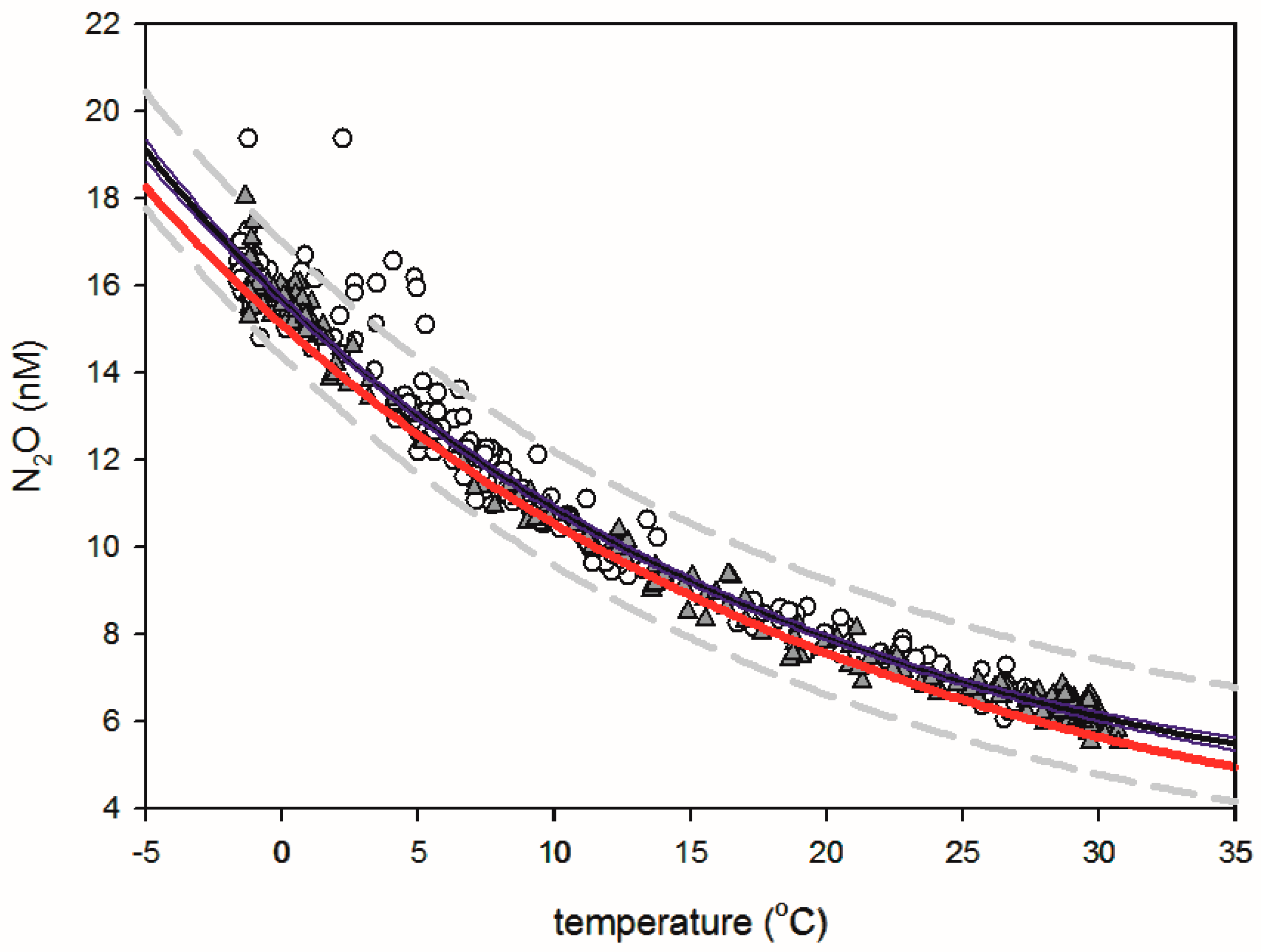
Zhan and Chen [28] documented the exponential decay relationship between the N2O concentration and surface seawater temperature (SST). In the present study, the data include those of the polar regions, which are plotted against SST and shown in Figure 3. Figure 3 shows that the correlation between these two datasets is significant (p < 0.0001), and the R2 is 0.9881, which is higher than that of 0.78 reported by Zhan and Chen [28]. The lower R2 of the latter regression may be due to the limited number of N2O samples and field SST and SSS data (used to calculate the N2O concentration) available to Zhan and Chen [28]. There are some data above the 95% prediction band, which are from the Bering Strait during the 4th Arctic Expedition.
The red curve in Figure 3 is the fitting curve of the N2O equilibrium concentration against temperature. The resulting fitting curve of the observed N2O clearly predicted a higher concentration of N2O over the equilibrium concentration. The correlation between the observed N2O data and the calculated equilibrium N2O concentration is shown in Figure 4. The figure shows that the observed N2O concentrations are significantly correlated with the theoretical equilibrium N2O concentrations. The high concentration end is more scattered than the low concentration end, suggesting that the high concentration end may be subject to an influence other than SST. Moreover, the intercept of the y-axis lays at approximately 0.4 ± 0.1 nM, suggesting that the observed N2O concentration is approximately 0.4 ± 0.1 nM higher than that of the equilibrium concentration. This difference results in oversaturations of 7% and 2% at low and high latitudes, respectively. Therefore, N2O is emitted to the atmosphere, and the tropical regions are more important sources than the polar and subpolar regions in this study.
3.2. Saturation Anomalies of Different Regions and Their Regulatory Factors
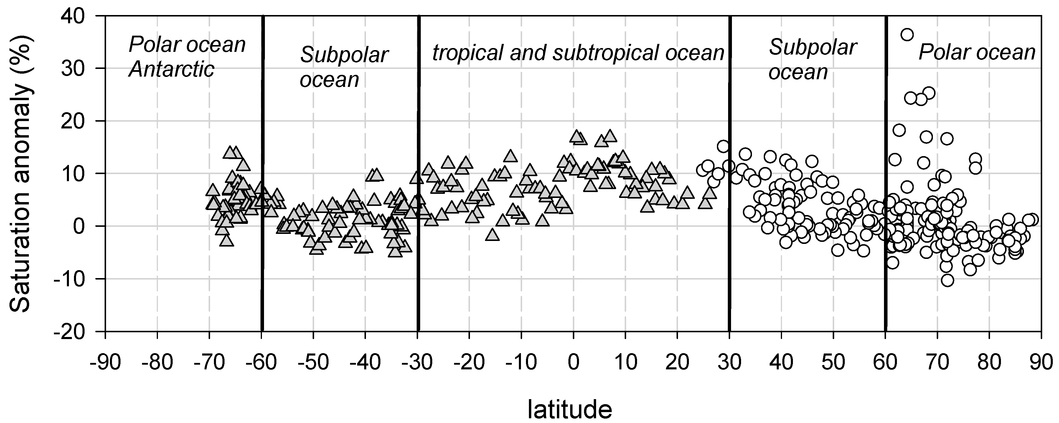
To reveal the influence of factors other than SST, the SA is calculated and discussed in the following sections. The SA values were plotted against latitude and is shown in Figure 5. The distribution of SA provides a clearer view of the source/sink characteristics than that provided by the concentration alone. The SA values range between −10% and 40% along the cruise tracks. Previous studies have also reported N2O undersaturation in surface waters [14,17,29]. The exchange rate of N2O is slower than that of heat, which can result in surface water N2O oversaturation or undersaturation, and the melting of sea ice in polar regions can dilute the surface water, resulting in surface water N2O undersaturation. As a whole, tropical surface seawater is oversaturated with N2O, whereas the polar oceans exhibit both N2O oversaturation and undersaturation. To make it easier to study the global N2O distributions, the distribution patterns of the whole cruise tracks were divided into different regional sections. The cruise tracks cover ocean regions with different characteristics, such as high-latitude cold polar regions, regions with strong westerly winds, and warm and high-temperature subtropical and tropical regions. These regional differences, together with the distribution patterns of N2O in the surface water, enable the study area to be divided into three regions, namely, the tropical/subtropical ocean (30° N–30° S), the subpolar oceans (30° N–60° N, 30° S–60° S) and the polar oceans (>60° N and >60° S).
3.2.1. Tropical and Subtropical Seas
The distribution of N2O between 30° N and 30° S is shown in Figure 5. The SA values range between −2% and 18%, with an average value of approximately 8%. Since the precision of this method is ~2%, the tropical/subtropical region shows the characteristics of a source of N2O.
This phenomenon is similar to that observed in other studies in both the Atlantic [30] and Pacific oceans [31]. The former study shows an N2O oversaturation of ~113% in the equatorial Atlantic due to equatorial upwelling, whereas the latter shows a somewhat elevated N2O level, even though the upwelling is less intense in the western Pacific. Although a similar phenomenon was present at the equator, the oversaturation mechanism along the cruise tracks is probably not identical to that of open oceans. Since the cruise tracks are located in marginal seas rather than the open oceans, the N2O SA along these cruise tracks may be subject to terrestrial influences.
During the 27th CHINARE, the highest SA value of approximately 17% was identified in the surface waters between 0° N and 10° N. Corresponding to this SA maximum is the SSS minimum (Figure 6). The lowest salinity during the 27th CHINARE is approximately 29.27 at the Equator. The cruise track passes through the Makassar Strait, where the surface water is freshened by the Mahakam River. Therefore, this result suggests that the surface water at the Makassar Strait during the 27th CHINARE may be influenced by river runoff. A river under anthropogenic influence is generally enriched in nitrogen-based nutrients, which are generally a significant source of N2O. The Mahakam River is a heavily polluted river and may be a source of N2O. This contribution can at least partly explain the observed corresponding high N2O SA and low salinity near the Equator. Therefore, the N2O oversaturation in tropical and subtropical seas may be a result of terrestrial influence.
Since the tropical and subtropical seas here may not represent the characteristics of the open ocean, the distribution pattern of N2O will not be further discussed.
3.2.2. Subpolar Oceans
In this study, the subpolar oceans are defined as the ocean areas at 30° N–60° N and 30° S–60° S.
There were two cruise tracks between 30° N and 60° N during the 4th CHINARE. R/V Xuelong set out from Shanghai, passed through the Japanese Sea and Okhotsk Sea, then headed to the Bering Sea in early July. After finishing the survey in the Arctic Ocean, the Xuelong returned to Shanghai via the western Bering Sea, western Pacific Ocean, and Japanese Sea, arriving in Shanghai in mid-September. Clear SA differences exist between Shanghai and the Aleutian Arc. The outbound cruise track shows a high SA value range between 1% and 14%, whereas the return cruise track shows an SA range between –5% and 7% (Figure 7a).
The seasonal thermal effect is one of the reasons underlying these SA differences. For example, between 30° N and 40° N, the cruise tracks almost overlap with each other; however, the SA value of the outbound cruise track is 9%, while that of the return cruise track is 2% (Figure 7a). Furthermore, the SST of the return cruise track is ~3 °C higher than that of the outbound cruise track (Figure 7b). Generally, increasing SST may result in temporary surface water oversaturation; however, a decrease in the SA along similar cruise tracks is observed. This phenomenon can be explained by a more rapid increase in SST from June to July than from July to September, as can be seen in the NOAA SST data [32]. The SST increases by approximately 4 °C and 1.5 °C on average from June to July and from July to September, respectively, in both the East China Sea and Japanese Sea. The sampling times are July and September; therefore, this temperature variability can account for the SA variability.
Another factor that influences the distribution pattern is the hydrographic structure. As seen from Figure 7b, decreasing SST can be observed between 40° N and 50° N along the outbound cruise track, where the cruise track crosses the Japanese Sea, enters the Okhotsk Sea via the Laperouse Strait, and arrives in the western Bering Sea. The Japanese Sea is a site of mixing of warm waters and cold waters, such as the Tsushima Current and Liman Current, which meet and form a polar front at approximately 45° N [33]. This polar front probably results in the salinity drop observed at this latitude (Figure 7c). Farther north, after the cruise track passes through the Laperouse Strait, the surface water reaches its lowest SST at 50° N, suggesting that the cruise track encounters the Oyashio Current. Corresponding to this decrease in SST, the SA value is found to be approximately zero. During its return, the R/V Xuelong passed through the western Pacific Ocean along the east coast of Hokkaido and entered the Japanese Sea via the Tsugaru Strait at approximately 42° N, where a temperature and salinity rise can be observed in the data (Figure 7c). A minor SA value increase accompanies the increase in temperature and salinity. The above phenomenon indicates that the N2O in cold water masses tends to be in an equilibrium state with the atmosphere, whereas the N2O in warm water masses tends to be oversaturated.
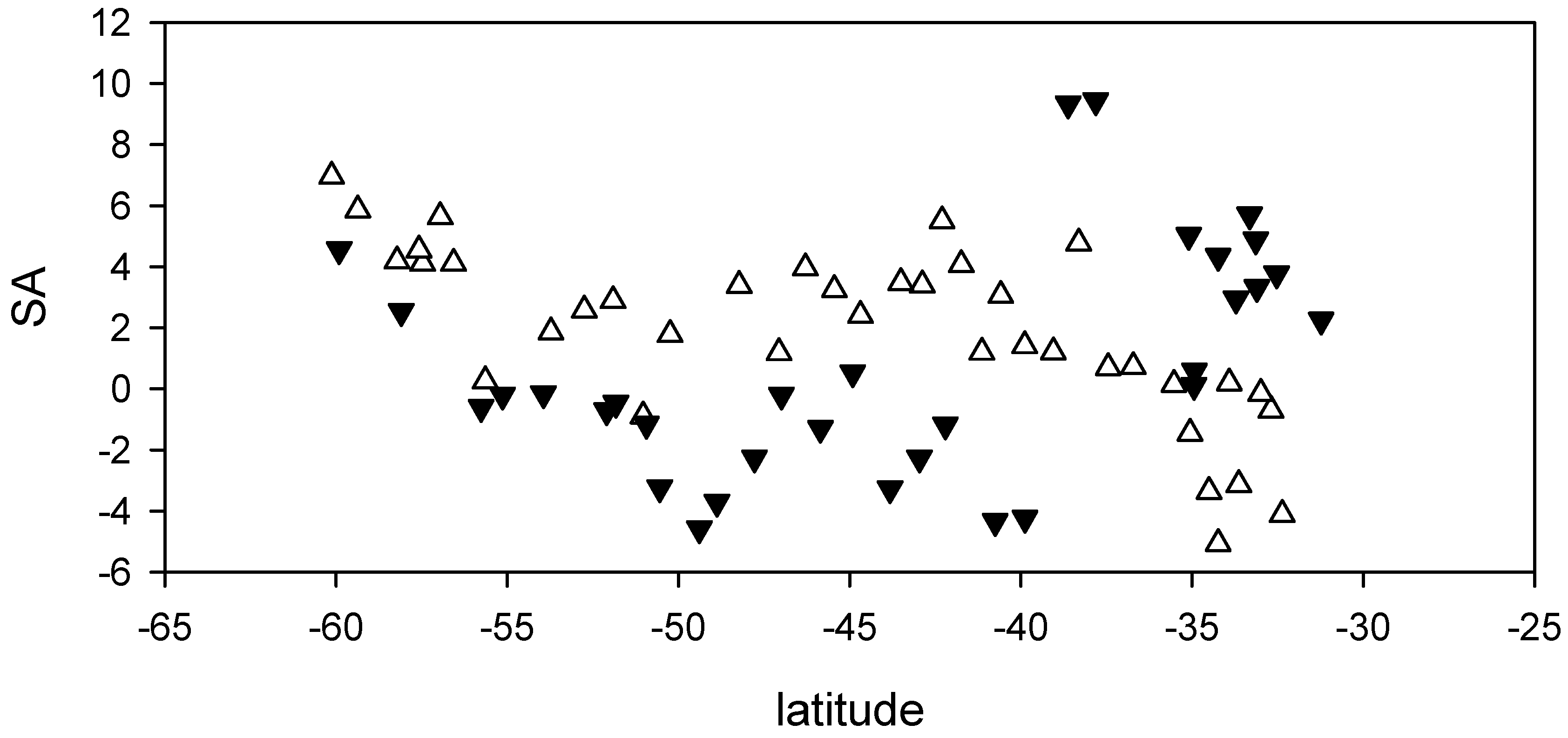
In the Southern Ocean, the surface water is near equilibrium with the atmosphere, as evidenced by both the southward and northward cruise tracks. Nevertheless, an SA value difference exists between the southward and northward cruise tracks. This phenomenon can be at least partly explained as the result of seasonal surface water temperature variations. Zhan and Chen [28] showed that the SA values of the surface water in the same study region ranged from approximately –10% in the south to approximately 40% on the Australia continental shelf, which they concluded to mainly be a result of the seasonal thermal effect. In the present study, the SA value ranged between approximately –5% and 10% (Figure 5), which is a smaller range than that reported by Zhan and Chen [28] and is probably due to the improvement of the precision and accuracy of the method and the availability of field SST and SSS data. Moreover, the distribution patterns of surface water SA can be subdivided into three latitude intervals according to differences between the two cruise tracks, i.e., south of 55° S, between 55° S and 40° S, and north of 40° S (Figure 8). South of 55° S, the SA of the surface water increases southward, which may result from Circumpolar Deep Water (CDW) upwelling or other local sources, which will be further discussed in the following section. Between 55° S and 40° S, the average SA value along the southward cruise track is approximately 2–3%, while that along the northward cruise track is approximately –2%, corresponding to the increasing SST and decreasing SST during the early and late summer, respectively. The SA value north of 40° S is unexplainable according to the available data. The trend in this region is opposite that of the intermediate section: the SA values are negative along the southward cruise track and positive along the northward cruise track, despite the SST increases and decreases at this latitude interval in October to November and in February to March, respectively, according to the SST data available online [32]. If an average SA value of approximately –2% or 4% can be considered an equilibrium state, the SA value difference of approximately 6% and the trend of the distribution between the southward and northward cruise tracks suggest that there might be some unknown mechanism contributing to this difference. This intersection of SA distribution corresponds to latitudes where a subtropical front (STF) is present, suggesting that possible biological process differences in the subsurface waters might contribute to this difference. After summer production, the surface water is more enriched in N2O and has a relatively high SA of approximately 10% at 38° S as a result of biological production during the summer. However, to address this difference, further work needs to be done.
3.2.3. Polar Oceans
The distributions of N2O in the high-latitude Southern Ocean and Sub-Arctic/Arctic Ocean are quite different. As shown in Figure 5, the N2O SA value in the surface layer of the Sub-Arctic/Arctic Ocean follows the decreasing trend of the subpolar regions, except between 60° N and 70° N, where the surface water shows the highest oversaturation value of the cruise track and then continues decreasing to the highest latitude. The highest SA value of the cruise track is observed in the Bering Strait and on the Chukchi Sea continental shelf, where the water depth is approximately 60 m. Different studies have described the oversaturation of N2O in this region. The highest N2O saturation observed by Hirota, Ijiri, Komatsu, Ohkubo, Nakagawa and Tsunogai [16] was approximately 157% in continental shelf waters of the Bering Sea and Chukchi Sea; Zhang et al. [17] showed an oversaturation of 106–118% on the Chukchi Sea shelf south of 69° N; and Wu et al. [34] observed N2O oversaturation on the continental shelf between 65° N and 73° N during the 5th CHINARE, suggesting that the Bering Sea to Chukchi Sea shelf is a hotspot for N2O production.
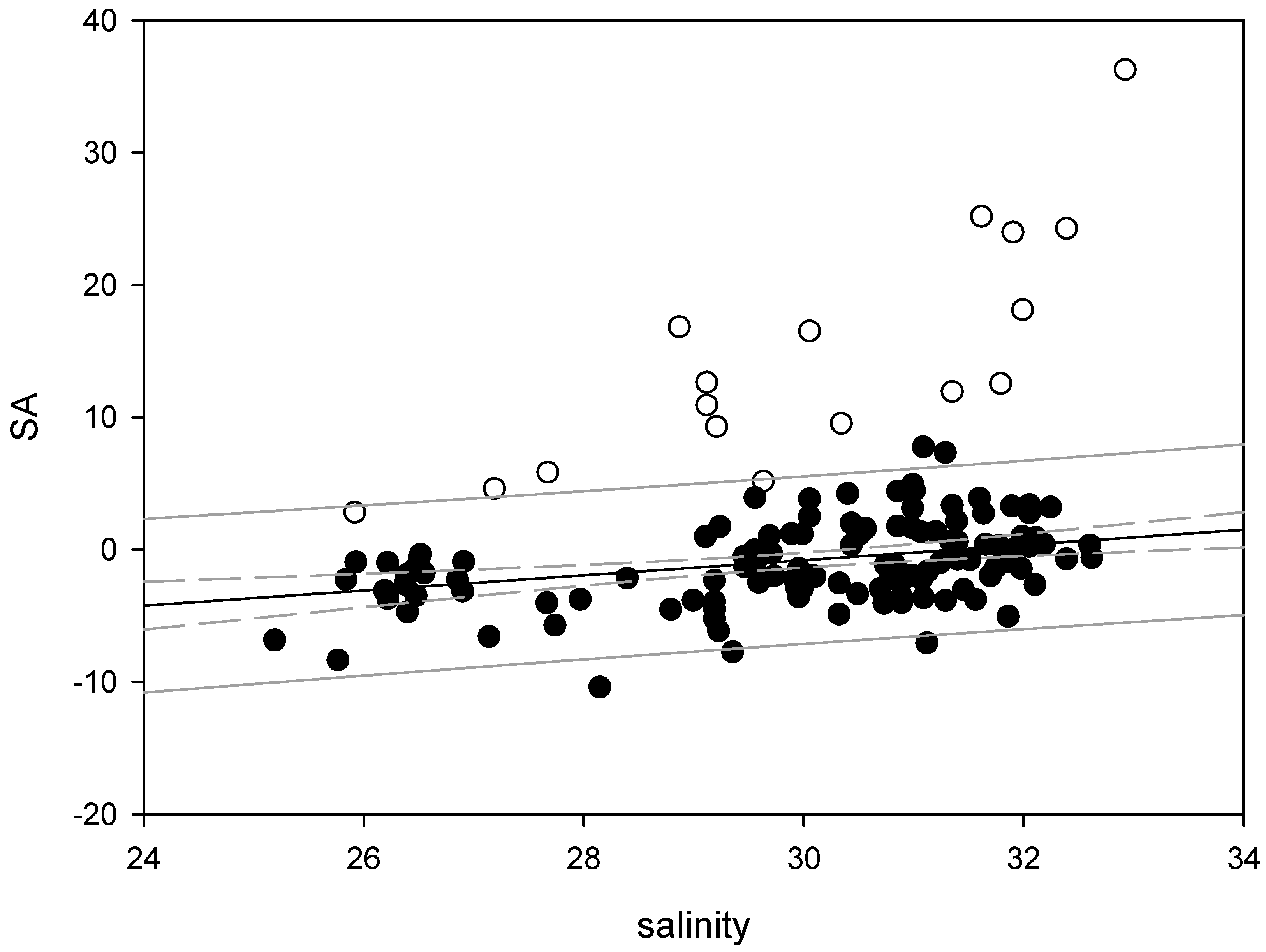
Farther north, surface water undersaturation can be observed. The lowest SA value is approximately –10%. There are reports of N2O undersaturation in the Arctic region. Wu et al. [34] and Zhang et al. [17] both showed undersaturation in the Canadian Basin, and Kitidis, Upstill-Goddard and Anderson [15] also found that the lowest N2O undersaturation of approximately 82% along a cruise track occurred in the Northwest Passage of the Arctic Ocean, which probably resulted from ice melt water dilution. In the present study, N2O undersaturation is also observed at high latitudes, and the lowest salinity in the surface water is present between 70° N and 80° N (Figure 6). When the SA is plotted against the SSS north of 60° N, a significant correlation is revealed (p = 0.0002, Figure 9) if the oversaturation observed at this latitude is excluded. Randall et al. [35] showed that the N2O in the Arctic sea ice is approximately 30% saturated, corresponding to the atmospheric levels. This finding effectively explains the N2O undersaturation observed in the low-salinity regions.
In the high-latitude Southern Ocean (>60° S), the water SA value distribution pattern is different from that of the high-latitude Arctic Ocean. Both oversaturation and undersaturation of N2O are present in the high-latitude Southern Ocean; however, the SA value is in the range of approximately −3 to 14%, a range that is narrower than that of the Arctic counterpart, which ranges from −10 to 36%. Zhan, Chen, Zhang, Yan, Li, Wu, Xu, Lin, Pan and Zhao [14] revealed a significant correlation between SA and salinity similar to that described above. However, no significant SA and SSS correlation can be identified in the high-latitude Southern Ocean, which indicates that the ice melting process may not be a significant factor influencing the surface water N2O equilibrium state.
The rather limited number of samples collected along the cruise track in the high-latitude Southern Ocean failed to capture the N2O undersaturation characteristics reported by Zhan et al. [14]. On the contrary, the limited data indicated possible oversaturation in the high-latitude Southern Ocean. Unlike on the Arctic/Sub-Arctic continental shelf, where sediment may be a source of N2O, there is no continental shelf at the latitude where the highest SA value was observed. This high oversaturation value may be the result of CDW upwelling, which was also observed by Zhan et al. [14]. In their work, Zhan et al. [14] observed that the highest N2O concentration occurred at approximately 200 m and corresponded to the lowest oxygen saturation level. This maximum N2O concentration may act as a source to the surface layer via upwelling or eddy diffusion between thermoclines. In the high-latitude Southern Ocean, a layer of warm surface water with a thickness of approximately 25 m occurs as a result of solar irradiance, and the N2O concentration in this surface layer is approximately 15.7 nmol·L−1. Below this layer, the temperature decreases to a minimum close to the freezing point then increases, which corresponds to the N2O concentration maximum of 22.4 nmol·L−1 at approximately 150 m. The warm surface layer and cold intermediate layer is a stable stratification structure, and there is no significant signal of subsurface water cropping out at the surface to cause the supersaturation observed during the 27th CHINARE. In addition to upwelling, eddy diffusion may contribute to the surface water layer. According to Li et al. [36], the flux resulting from eddy diffusion in this region is 0.18 μmol·m−2·d−1. Consequently, eddy diffusion does not appear to be able to sustain the supersaturation observed in the surface layer.
3.3. Air-Sea Fluxes
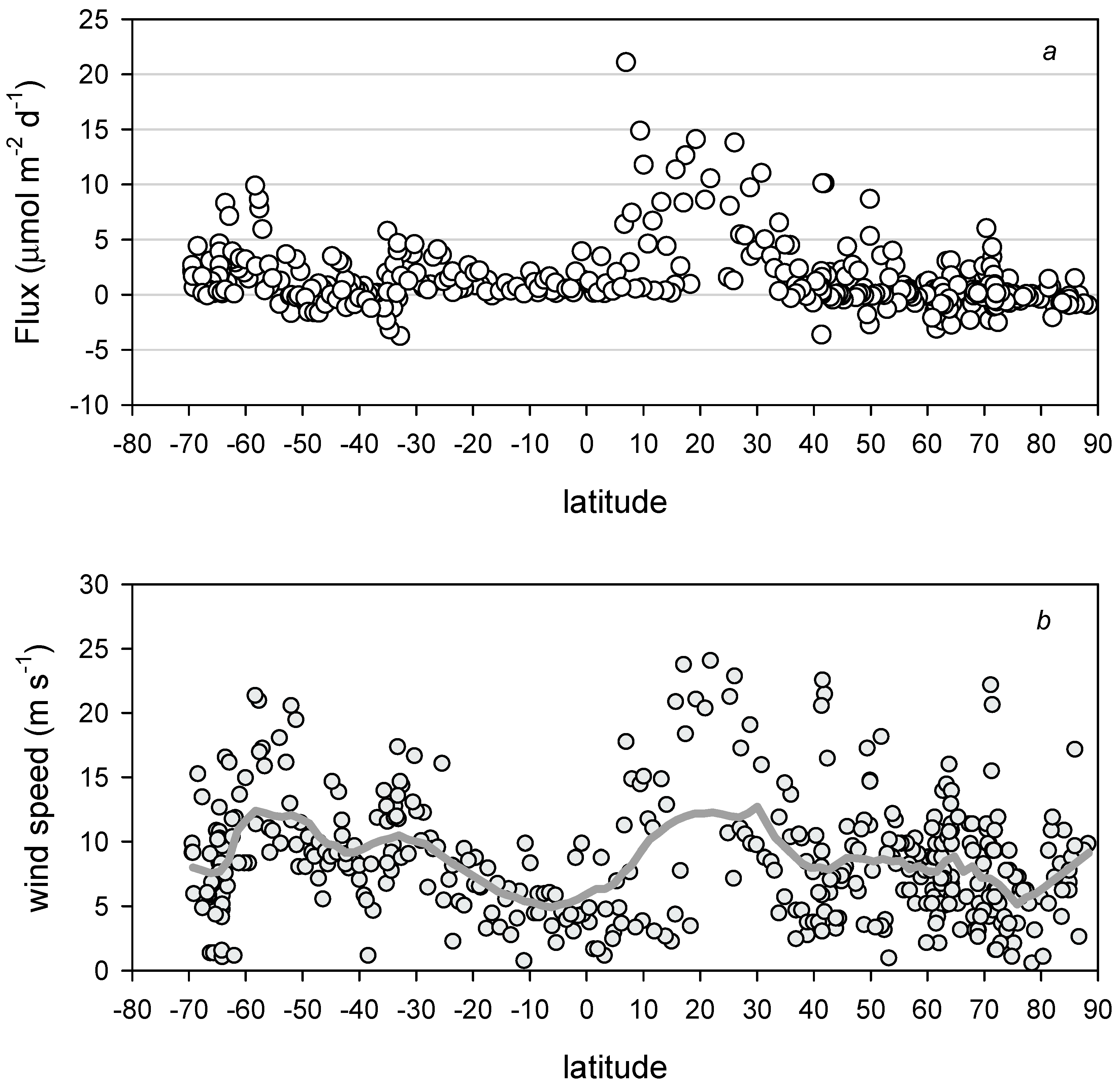
The N2O air-sea fluxes along the cruise tracks were calculated using Equations (2)–(4). The air-sea flux distribution pattern is shown in Figure 10a. The largest air-sea flux occurs in the tropical and subtropical regions defined in this study and is approximately 21.0 ± 4 μmol·m−2·d−1, observed near 10° N. Between 10° N and 30° N, the highest air-sea flux is approximately 14.8 ± 2.8 μmol·m−2·d−1; however, no high N2O air-sea flux is observed in the southern part of the tropical and subtropical areas (0° S–30° S). In the subpolar regions (30° S–60° S and 30° N–60° N), the air-sea flux in the north again shows a higher value than that in the Southern Ocean. Nevertheless, near the boundary between the southern polar and subpolar regions, a maximum air-sea N2O flux of approximately 10 μmol·m−2·d−1 is observed. Notably, the air-sea N2O flux of the northern polar region is not higher than that of its southern counterpart; instead, it shows a lower flux than that of the south, suggesting that the southern polar region may be a more important source to the atmosphere than the northern polar region. South of 60° S, the air-sea N2O flux reaches values higher than 5 μmol·m−2·d−1, which is higher than in the northern polar region, except for the relatively high flux over the Chukchi Sea continental shelf (~70° N).
Along the cruise tracks, the air-sea N2O fluxes do not exactly correspond to the surface water SA values. For example, high SA values in the subtropical and tropical regions do not result in high air-sea N2O fluxes all the time, as evidenced by the differences between the northern and southern subtropical and tropical regions. Both the northern and southern tropical and subtropical regions are oversaturated with N2O; however, high air-sea N2O fluxes mainly occur in the northern part. In the polar regions, the greatest N2O undersaturation is observed in the Arctic Ocean; however, no obvious sink characteristics are observed in the air-sea N2O flux distribution patterns in this region. In the southern polar region, the highest air-sea N2O fluxes are observed at approximately 60° S, but the highest SA value is present at approximately 65° S. The differences between the air-sea N2 fluxes and the SA distribution patterns suggest that the state of equilibrium of N2O in the surface water is the fundamental driver of the source/sink behavior in a certain area but that other factors influence the air-sea fluxes. Figure 10b shows the distribution of wind speed along the cruise tracks. The combination of wind speed and SA patterns together account for the air-sea flux patterns along the cruise tracks. Although a positive SA exists between 30° S and the equator, this region does not show air-sea N2O fluxes as high as that of the northern counterpart due to relatively lower wind speeds in this latitude interval. A similar phenomenon is also observed in the Arctic Ocean: here, the lowest negative SA value is observed, but the air-sea N2O flux is close to zero, which can be explained by the low wind speed in the Arctic Ocean. The highest air-sea N2O fluxes in the Southern Ocean are observed near 60° S rather than 65° S, where the highest SA value is present, because the highest wind speeds occur between 50° S and 60° S.
From these distribution patterns, the following can be concluded: (1) the tropical and subtropical regions are sources of atmospheric N2O, probably due to the coastal and continental shelf N2O production. Under high wind speed conditions, the highest sea-to-air N2O flux is ~21.0 ± 3.9 μmol·m−2·d−1. (2) The greatest N2O undersaturation is identified in the Arctic Ocean; however, due to the relatively low wind speeds in this region, no significant N2O sink is observed. (3) Along our cruise track, the Southern Ocean exhibits oversaturation at some stations; however, Zhan et al. [14] observed undersaturation in the shelf water. The Southern Ocean in this study does not behave as predicted by Nevison, Weiss and Erickson III [4] and Suntharalingam and Sarmiento [5], which may be due to differences in the data from different cruise tracks. In our study, the high air-sea N2O fluxes mainly occur at approximately 60° S. The results of sampling during the 27th CHINARE show that eddy diffusion is approximately 0.18 μmol·m−2·d−1, whereas the air-sea fluxes of this region is approximately 10 μmol·m−2·d−1. Consequently, eddy diffusion cannot account for the air-sea N2O flux. Therefore, upwelling, or even in situ production, may act as the source of the N2O outgassing at this latitude. However, to further assess the source/sink characteristics of the Southern Ocean, further work is needed.
4. Conclusions
The first large-scale, Arctic-to-Antarctic profiles of N2O in the surface water and the air-sea N2O flux are presented and discussed in this work. The results show the following: (1) N2O is oversaturated in the tropical and subtropical regions (30° N–30° S) along the cruise tracks, probably resulting from coastal influences, and higher air-sea fluxes are present in the Northern Hemisphere than in the Southern Hemisphere, which may be the result of high wind speeds in the Northern Hemisphere. The maximum air-sea flux is approximately 21.0 ± 3.9 μmol·m−2·d−1. (2) The distribution patterns of N2O in the sub-polar regions (30° N–60° N, 30° S–60° S) transition from oversaturated to approximate equilibrium with the atmosphere, and the boundaries generally correspond to frontal structures. Seasonal temperature variability and cruise track differences can account for the surface water SA variability, suggesting that most of this variability may be dominated by physical processes. (3) The distributions of N2O in the high-latitude Southern Ocean and Arctic Ocean (>60° N and 60° S) have contrary patterns. With the exception of surface water of the continental shelf hotspot, the Arctic Ocean surface water is undersaturated with N2O, possibly due to ice melt and river discharge dilution. However, the air-sea flux is close to zero because of the low wind speeds. In contrast, the high-latitude Southern Ocean is oversaturated with N2O, with an SA range between −3% and 14%. Upwelling or local production may contribute to this oversaturation. However, because the wind speed decreases southward, the oversaturation and undersaturation do not result in significant source or sink characteristics in the high-latitude Southern Ocean.
Acknowledgments
This work was funded by the National Natural Science Foundation of China (Grant Nos. 41230529 and 41476172), Chinese Projects for Investigations and Assessments of the Arctic and Antarctic (Grants Nos. CHINARE2012-15 for 01–04, 02–01, and 03–04), and the Chinese International Cooperation Projects (S2015GR1195, IC201201, IC201308, and IC201513). We would like to thank the officers, captain and crew of the R/V Xuelong for help with the sampling. Finally, we thank the anonymous reviewers for their helpful comments on the manuscript.
Author Contributions
Liyang Zhan contributes the idea and conducts paper writing, Man Wu contribute idea and conducted analysis; Liqi Chen contributes idea, discussion and suggestion on paper writing; Jixia Zhang conducted parts of analysis; Yuhong Li and Jian Liu attended the field work and conducted part of the analysis.
Conflicts of Interest
The author declare no conflict of interest.
References
- Khalil, M.A.K.; Rasmussen, R.A.; Shearer, M.J. Atmospheric nitrous oxide: Patterns of global change during recent decades and centuries. Chemosphere 2002, 47, 807–821. [Google Scholar] [CrossRef]
- Clark, D.; Brown, I.; Rees, A.; Somerfield, P.; Miller, P. The influence of ocean acidification on nitrogen regeneration and nitrous oxide production in the North-West European shelf sea. Biogeosci. Discuss. 2014, 11, 3113–3165. [Google Scholar] [CrossRef]
- Ravishankara, A.R.; Daniel, J.S.; Portmann, R.W. Nitrous oxide (N2O): The dominant ozone-depleting substance emitted in the 21st century. Science 2009, 326, 123. [Google Scholar] [CrossRef] [PubMed]
- Nevison, C.D.; Weiss, R.F.; Erickson, D.J. Global oceanic emissions of nitrous oxide. J. Geophys. Res. 1995, 100, 15809–15820. [Google Scholar] [CrossRef]
- Suntharalingam, P.; Sarmiento, J.L. Factors governing the oceanic nitrous oxide distribution: Simulations with an ocean general circulation model. Glob. Biogeochem. Cycles 2000, 14, 429–454. [Google Scholar] [CrossRef]
- Freing, A.; Wallace, D.W.; Bange, H.W. Global oceanic production of nitrous oxide. Philos. Trans. R. Soc. Lond. B Biol. Sci. 2012, 367, 1245–1255. [Google Scholar] [CrossRef] [PubMed] [Green Version]
- Arevalo-Martinez, D.L.; Kock, A.; Loscher, C.R.; Schmitz, R.A.; Bange, H.W. Massive nitrous oxide emissions from the tropical South Pacific Ocean. Nat. Geosci. 2015, 8, 530–533. [Google Scholar] [CrossRef]
- Bange, H.W.; Rapsomanikis, S.; Andreae, M.O. Nitrous oxide emissions from the Arabian Sea. Geophys. Res. Lett. 1996, 23, 3175–3178. [Google Scholar] [CrossRef] [Green Version]
- Bouwman, A.F.; Van der Hoek, K.W.; Olivier, J.G.J. Uncertainties in the global source distribution of nitrous oxide. J. Geophys. Res. 1995, 100, 2785–2800. [Google Scholar] [CrossRef]
- Nevison, C.D.; Keeling, R.F.; Weiss, R.F.; Popp, B.N.; Jin, X.; Fraser, P.J.; Porter, L.W.; Hess, P.G. Southern ocean ventilation inferred from seasonal cycles of atmospheric N2O and O2/N2 at Cape Grim, Tasmania. Tellus B 2005, 57, 218–229. [Google Scholar] [CrossRef]
- Huang, J.; Golombek, A.; Prinn, R.; Weiss, R.; Fraser, P.; Simmonds, P.; Dlugokencky, E.J.; Hall, B.; Elkins, J.; Steele, P. Estimation of regional emissions of nitrous oxide from 1997 to 2005 using multinetwork measurements, a chemical transport model, and an inverse method. J. Geophys. Res. 2008, 113, D17313. [Google Scholar] [CrossRef]
- Hirsch, A.I.; Michalak, A.M.; Bruhwiler, L.M.; Peters, W.; Dlugokencky, E.J.; Tans, P.P. Inverse modeling estimates of the global nitrous oxide surface flux from 1998–2001. Glob. Biogeochem. Cycles 2006, 20. [Google Scholar] [CrossRef]
- Rees, A.P.; Owens, N.J.P.; Upstill-Goddard, R.C. Nitrous oxide in the Bellingshausen sea and drake passage. J. Geophys. Res. 1997, 102, 3383–3392. [Google Scholar] [CrossRef]
- Zhan, L.; Chen, L.; Zhang, J.; Yan, J.; Li, Y.; Wu, M.; Xu, S.; Lin, Q.; Pan, J.; Zhao, J. Austral summer N2O sink and source characteristics and their impact factors in Prydz Bay, Antarctica. J. Geophys. Res. Oceans 2015, 120, 5836–5849. [Google Scholar] [CrossRef]
- Kitidis, V.; Upstill-Goddard, R.C.; Anderson, L.G. Methane and nitrous oxide in surface water along the North-West passage, Arctic Ocean. Mar. Chem. 2010, 121, 80–86. [Google Scholar] [CrossRef]
- Hirota, A.; Ijiri, A.; Komatsu, D.D.; Ohkubo, S.B.; Nakagawa, F.; Tsunogai, U. Enrichment of nitrous oxide in the water columns in the area of the Bering and Chukchi seas. Mar. Chem. 2009, 116, 47–53. [Google Scholar] [CrossRef]
- Zhang, J.; Zhan, L.; Chen, L.; Li, Y.; Chen, J. Coexistence of nitrous oxide undersaturation and oversaturation in the surface and subsurface of the western Arctic Ocean. J. Geophys. Res. Oceans 2015. [Google Scholar] [CrossRef]
- Butler, J.H.; Elkins, J.W. An automated technique for the measurement of dissolved N2O in natural waters. Mar. Chem. 1991, 34, 47–61. [Google Scholar] [CrossRef]
- Bange, H.W.; Rapsomanikis, S.; Andreae, M.O. Nitrous oxide in coastal waters. Glob. Biogeochem. Cycles 1996, 10, 197–207. [Google Scholar] [CrossRef] [Green Version]
- Cohen, Y. Shipboard measurement of dissolved nitrous oxide in sea water by electron capture gas chromatography. Anal. Chem. 1977, 49, 1238–1240. [Google Scholar] [CrossRef]
- Capelle, D.W.; Dacey, J.W.; Tortell, P.D. An automated, high through-put method for accurate and precise measurements of dissolved nitrous-oxide and methane concentrations in natural waters. Limnol. Oceanogr. Methods 2015, 13, 345–355. [Google Scholar] [CrossRef]
- Zhan, L.Y.; Chen, L.Q.; Zhang, J.X.; Lin, Q. A system for the automated static headspace analysis of dissolved N2O in seawater. Int. J. Environ. Anal. Chem. 2012, 93, 828–842. [Google Scholar] [CrossRef]
- Weiss, R.F.; Price, B.A. Nitrous oxide solubility in water and seawater. Mar. Chem. 1980, 8, 347–359. [Google Scholar] [CrossRef]
- Combined Nitrous Oxide Data from the NOAA/ESRL Global Monitoring Division. Available online: www.esrl.noaa.gov/gmd/hats (accessed on 15 July 2017).
- Jiang, L.Q.; Cai, W.J.; Wanninkhof, R.; Wang, Y.; Luger, H. Air-sea CO2 fluxes on the US South Atlantic Bight: Spatial and seasonal variability. J. Geophys. Res. Oceans 2008, 113, C07019. [Google Scholar] [CrossRef]
- Wanninkhof, R. Relationship between wind speed and gas exchange. J. Geophys. Res. 1992, 97, 7373–7382. [Google Scholar] [CrossRef]
- Wanninkhof, R. Relationship between wind speed and gas exchange over the ocean revisited. Limnol. Oceanogr. Methods 2014, 12, 351–362. [Google Scholar] [CrossRef]
- Zhan, L.; Chen, L. Distributions of N2O and its air-sea fluxes in seawater along cruise tracks between 30° S–67° S and in Prydz Bay, Antarctica. J. Geophys. Res. 2009, 114, C03019. [Google Scholar] [CrossRef]
- Butler, J.; Elkins, J.; Brunson, C.; Egan, K.; Thompson, T.; Conway, T.; Hall, B. Trace Gases in and over the West Pacific and East Indian Oceans during the El Niño-Southern Oscillation Event of 1987. Available online: http://adsabs.harvard.edu/abs/1988saga.rept.....B (accessed on 15 July 2017).
- Walter, S.; Bange, H.W.; Wallace, D.W.R. Nitrous oxide in the surface layer of the tropical North Atlantic Ocean along a west to east transect. Geophys. Res. Lett. 2004, 31, L23S07. [Google Scholar] [CrossRef]
- Butler, J.; Elkins, J.; Thompson, T.; Egan, K. Tropospheric and dissolved N2O of the west Pacific and east Indian Oceans during the El Niño Southern Oscillation event of 1987. J. Geophys. Res. 1989, 94, 14865–14877. [Google Scholar] [CrossRef]
- Asia-Pacific Data-Research Cneter of the IPRC. Available online: http://apdrc.soest.hawaii.edu/data/data.phphttp://apdrc.soest.hawaii.edu/data/data.php (accessed on 15 July 2017).
- Tomczak, M.; Godfrey, J.S. Regional Oceanography: An Introduction, 1st ed.; Elsevier Science Ltd.: New York, NY, USA, 1994. [Google Scholar]
- Wu, M.; Chen, L.; Zhan, L.; Zhang, J.; Li, Y.; Liu, J. Spatial Variability and Factors Influencing the Air-Sea N2O Flux in the Bering Sea, Chukchi Sea and Chukchi Abyssal Plain. Atmosphere 2017, 8, 65. [Google Scholar] [CrossRef]
- Randall, K.; Scarratt, M.; Levasseur, M.; Michaud, S.; Xie, H.; Gosselin, M. First measurements of nitrous oxide in Arctic sea ice. J. Geophys. Res. Oceans 2012, 117. [Google Scholar] [CrossRef]
- Li, Y.H.; Peng, T.H.; Broecker, W.S.; Oestlund, H. The average vertical mixing coefficient for the oceanic thermocline. Tellus B 1984, 36, 212–217. [Google Scholar] [CrossRef]
Figure 1.
The cruise tracks of the 4th Chinese National Arctic Research Expedition and the 27th Chinese Antarctic Research Expedition. The background color of the map is bathymetry.
Figure 1.
The cruise tracks of the 4th Chinese National Arctic Research Expedition and the 27th Chinese Antarctic Research Expedition. The background color of the map is bathymetry.
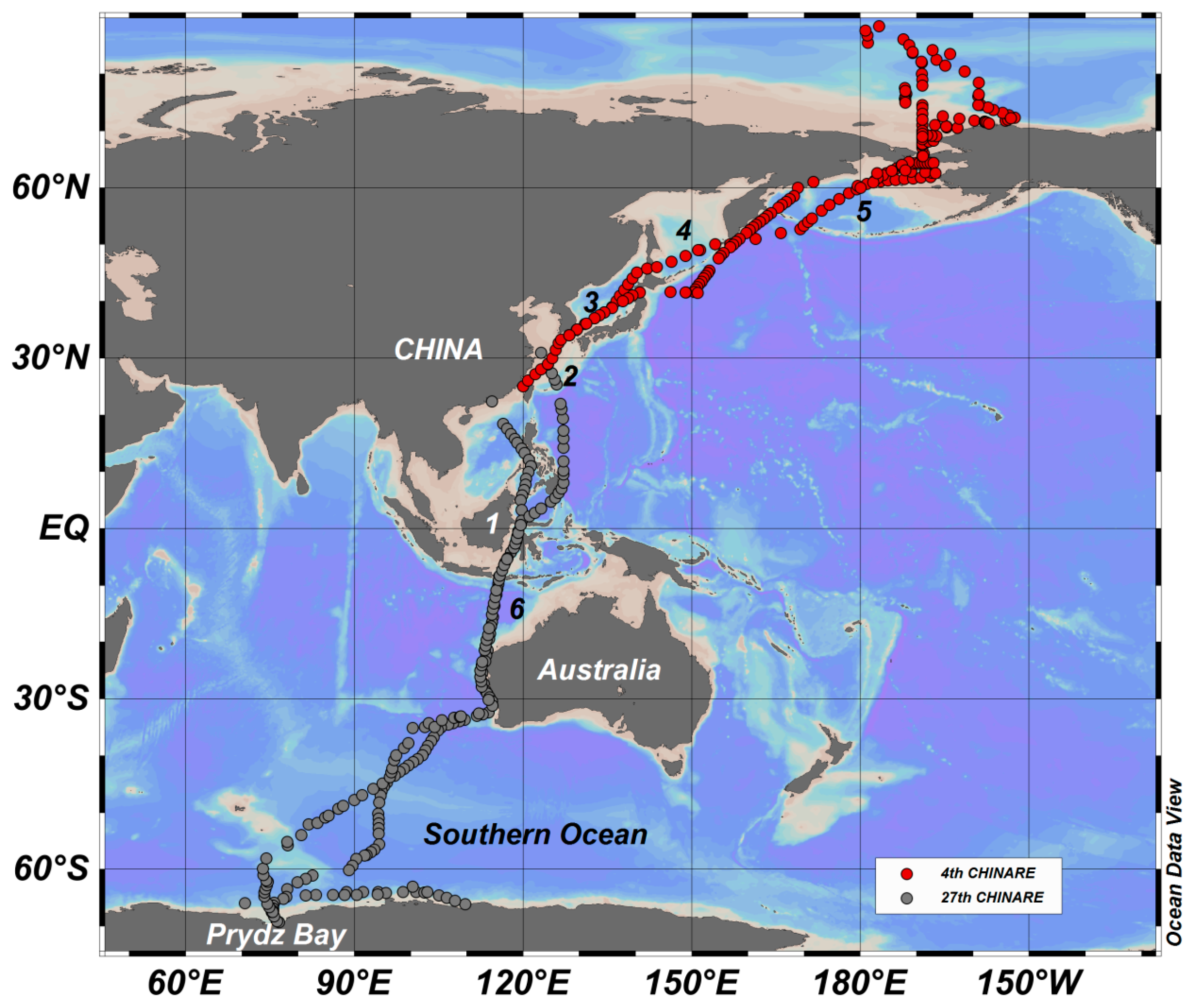
Figure 2.
The distribution patterns of the 4th Chinese National Arctic Research Expedition (empty circles) and the 27th Chinese Antarctic Research Expedition (gray triangles). High concentrations and relatively low concentrations of N2O were observed at high latitudes and low latitudes, respectively.
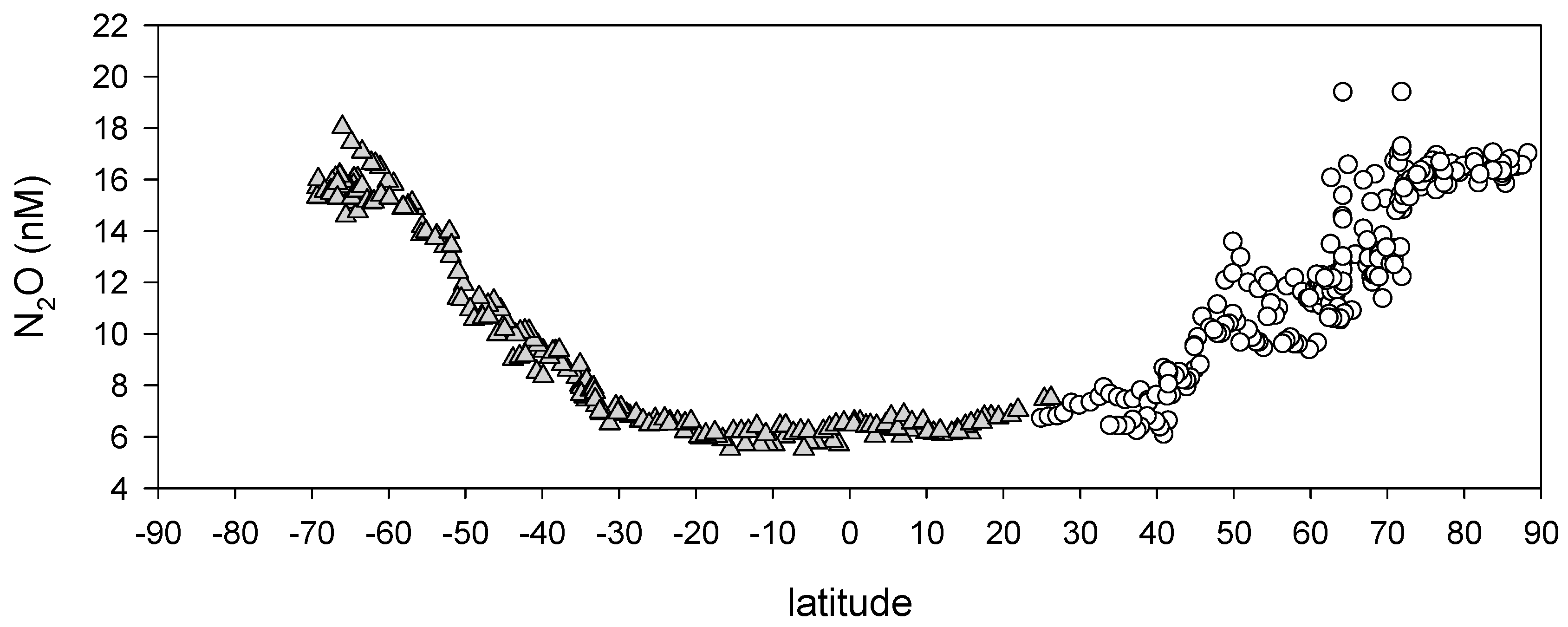
Figure 3.
Exponential decay of N2O concentration against surface seawater temperature. y = (2.3703 ± 0.1777) + (13.017 ± 0.1711)exp[(−0.459 ± 0.0011)·x] (y = (2.4704 ± 0.0947) + (12.7443 ± 0.0888)exp[(−0.459 ± 0.0007)·x]) (p < 0.0001). The open circles and gray triangles are data obtained during the 4th and 27th Chinese National Antarctic Research Expedtion. The regression line is shown as the black line, and the 95% prediction band is shown as the gray dashed line. The red line is the regression line of the equilibrium concentration against surface seawater temperature.

Figure 4.
Correlation between observed N2O concentration (N2Oob) and equilibrium N2O concentration (N2Oeq) in the surface water of the 4th Chinese National Arctic Research Expedition and the 27th Chinese Antarctic Research Expedition. A significant correlation (y = 0.3954 ± 0.0601 + (0.9865 ± 0.0053)·x) between N2Oob and N2Oeq is observed (p < 0.0001).
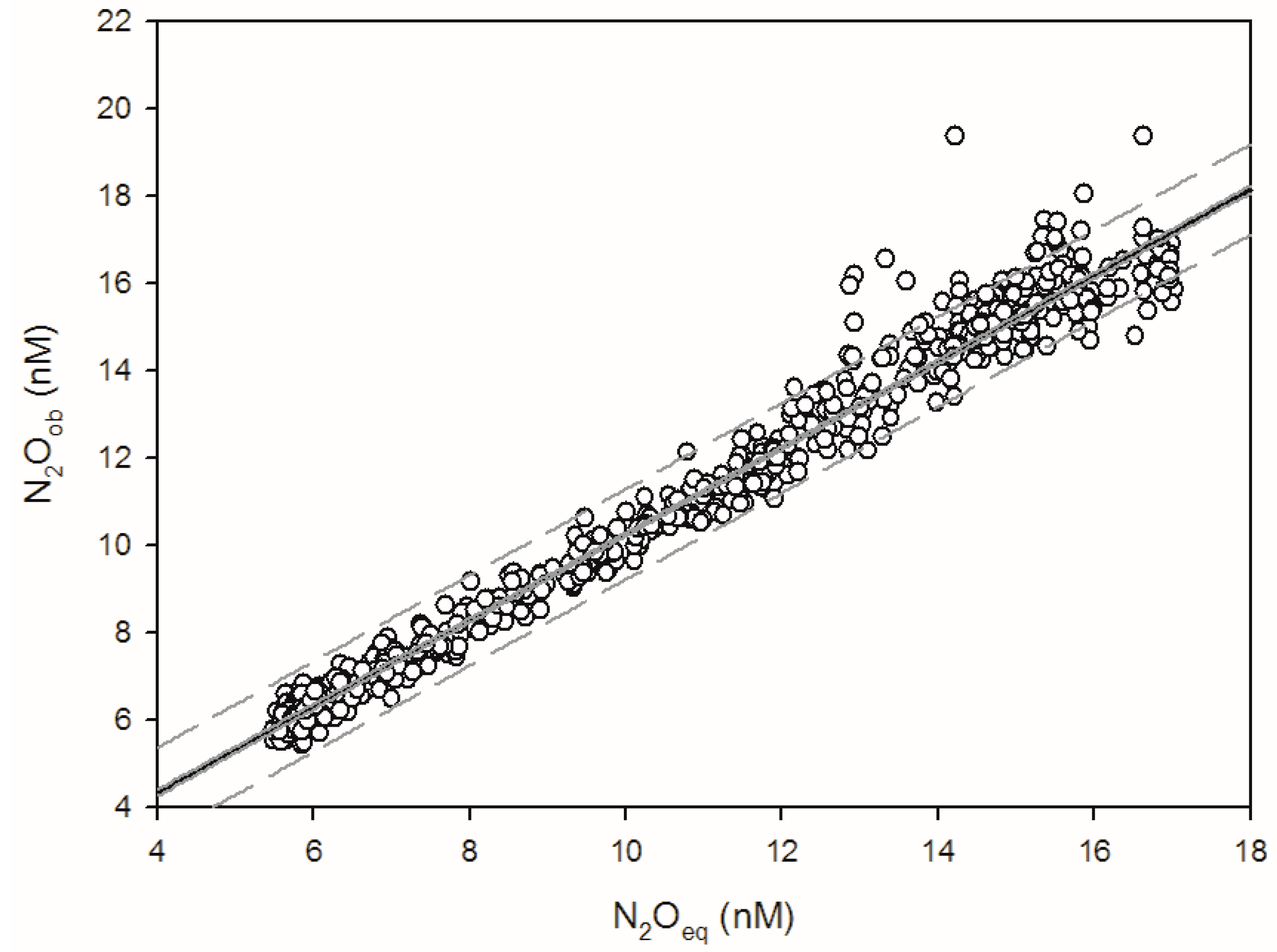
Figure 5.
Saturation Anomaly values along the cruise tracks of the 4th Chinese National Arctic Research Expedition (empty circles) and the 27th Chinese Antarctic Research Expedition (gray triangles).
Figure 5.
Saturation Anomaly values along the cruise tracks of the 4th Chinese National Arctic Research Expedition (empty circles) and the 27th Chinese Antarctic Research Expedition (gray triangles).

Figure 6.
Surface salinity along the cruise tracks of the 4th Chinese National Arctic Research Expedition (empty circles) and the 27th Chinese Antarctic Research Expedition (gray triangles). Low salinity is identified near the Equator, at 30° N and at 75° N. The first two low salinity regions are influenced by river runoff, and the third may be influenced by ice melt water and river runoff.
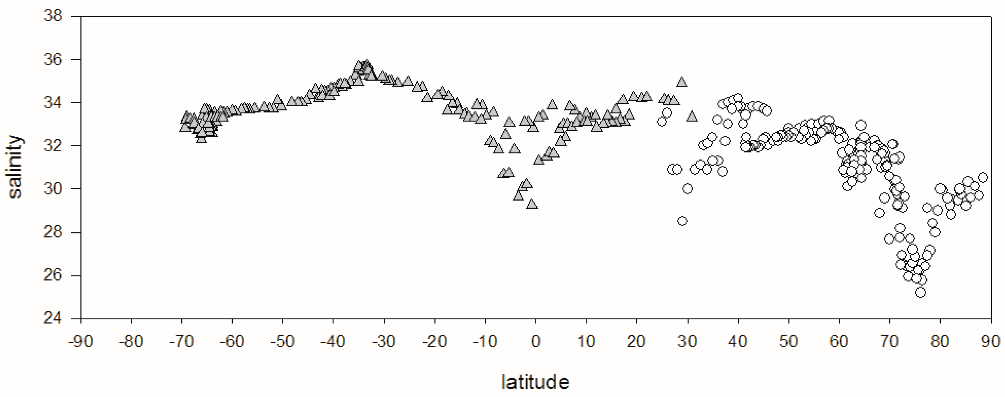
Figure 7.
(a) The SA on the northward (open circles) and southward (solid dots) cruise tracks of the 4th Chinese National Arctic Research Expedition; (b) The surface water temperature on the northward (open circles) and southward (solid dots) cruise tracks of the 4th Chinese National Arctic Research Expedition; (c) The surface water salinity on the northward (open circles) and southward (solid dots) cruise tracks of the 4th Chinese National Arctic Research Expedition.
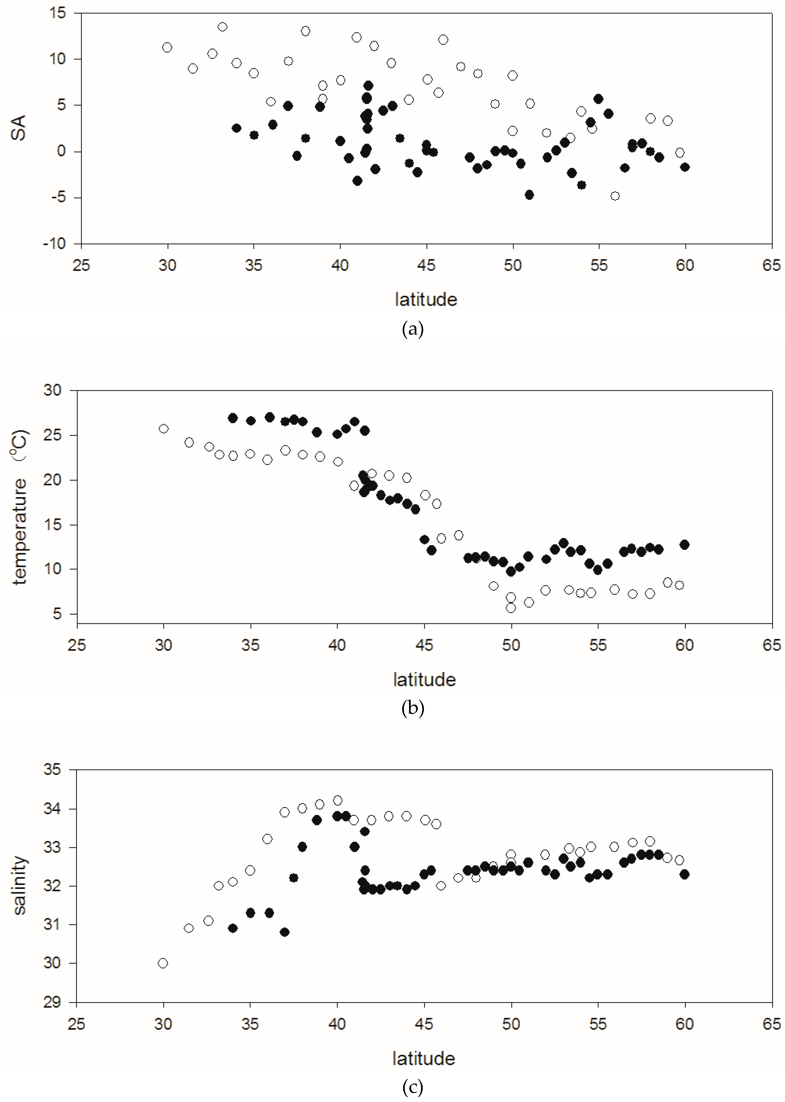
Figure 8.
Distribution of SA values along the southward (solid triangles) and northward (open triangles) tracks of the 27th Chinese Antarctic Research Expedition.
Figure 8.
Distribution of SA values along the southward (solid triangles) and northward (open triangles) tracks of the 27th Chinese Antarctic Research Expedition.

Figure 9.
Correlation between SA and salinity in the Arctic Ocean. The open circles represent the stations associated with the N2O hotspot on the continental shelf. The solid dots represent the stations less affected by the continental shelf hotspot. The SA and salinity of the solid dot stations are significantly correlated with each other in this region.

Figure 10.
(a) The in situ air-sea N2O fluxes and (b) the in situ wind speed along the cruise tracks of both the 4th Chinese National Arctic Research Expedition and the 27th Chinese Antarctic Research Expedition.
Figure 10.
(a) The in situ air-sea N2O fluxes and (b) the in situ wind speed along the cruise tracks of both the 4th Chinese National Arctic Research Expedition and the 27th Chinese Antarctic Research Expedition.
© 2017 by the authors. Licensee MDPI, Basel, Switzerland. This article is an open access article distributed under the terms and conditions of the Creative Commons Attribution (CC BY) license (http://creativecommons.org/licenses/by/4.0/).
Share and Cite
MDPI and ACS Style
Zhan, L.; Wu, M.; Chen, L.; Zhang, J.; Li, Y.; Liu, J. The Air-Sea Nitrous Oxide Flux along Cruise Tracks to the Arctic Ocean and Southern Ocean. Atmosphere 2017, 8, 216. https://doi.org/10.3390/atmos8110216
AMA Style
Zhan L, Wu M, Chen L, Zhang J, Li Y, Liu J. The Air-Sea Nitrous Oxide Flux along Cruise Tracks to the Arctic Ocean and Southern Ocean. Atmosphere. 2017; 8(11):216. https://doi.org/10.3390/atmos8110216
Chicago/Turabian StyleZhan, Liyang, Man Wu, Liqi Chen, Jixia Zhang, Yuhong Li, and Jian Liu. 2017. "The Air-Sea Nitrous Oxide Flux along Cruise Tracks to the Arctic Ocean and Southern Ocean" Atmosphere 8, no. 11: 216. https://doi.org/10.3390/atmos8110216
Note that from the first issue of 2016, this journal uses article numbers instead of page numbers. See further details here.