Estimating Uncertainty in Global Mercury Emission Source and Deposition Receptor Relationships

 , , , ,
Abstract
:1. Introduction
2. Materials and Methods
3. Results
Uncertainty in the Source-Receptor Matrix
4. Discussion
Acknowledgments
Author Contributions
Conflicts of Interest
Abbreviations
| NCIAM | normalised confidence interval amplitude for the mean |
References
- Fitzgerald, W.F.; Engstrom, D.R.; Mason, R.P.; Nater, E.A. The case for atmospheric mercury contamination in remote areas. Environ. Sci. Technol. 1998, 32, 1–7. [Google Scholar] [CrossRef]
- Gustin, M.S.; Evers, D.C.; Bank, M.S.; Hammerschmidt, C.R.; Pierce, A.; Basu, N.; Blum, J.; Bustamante, P.; Chen, C.; Driscoll, C.T.; et al. Importance of Integration and Implementation of Emerging and Future Mercury Research into the Minamata Convention. Environ. Sci. Technol. 2016, 50, 2767–2770. [Google Scholar] [CrossRef] [PubMed]
- De Simone, F.; Gencarelli, C.N.; Hedgecock, I.M.; Pirrone, N. A modeling comparison of mercury deposition from current anthropogenic mercury emission inventories. Environ. Sci. Technol. 2016, 50, 5154–5162. [Google Scholar] [CrossRef] [PubMed]
- Bullock, O.R.; Atkinson, D.; Braverman, T.; Civerolo, K.; Dastoor, A.; Davignon, D.; Ku, J.Y.; Lohman, K.; Myers, T.C.; Park, R.J.; et al. The North American Mercury Model Intercomparison Study (NAMMIS): Study description and model-to-model comparisons. J. Geophys. Res. 2008, 113, 1–17. [Google Scholar] [CrossRef]
- Lin, C.J.; Pongprueksa, P.; Lindberg, S.E.; Pehkonen, S.O.; Byun, D.; Jang, C. Scientific uncertainties in atmospheric mercury models I: Model science evaluation. Atmos. Environ. 2006, 40, 2911–2928. [Google Scholar] [CrossRef]
- Pongprueksa, P.; Lin, C.J.; Lindberg, S.E.; Jang, C.; Braverman, T.; Bullock, O.R.; Ho, T.C.; Chu, H.W. Scientific uncertainties in atmospheric mercury models III: Boundary and initial conditions, model grid resolution, and Hg (II) reduction mechanism. Atmos. Environ. 2008, 42, 1828–1845. [Google Scholar] [CrossRef]
- Dvonch, J.; Graney, J.; Marsik, F.; Keeler, G.; Stevens, R. An investigation of source–receptor relationships for mercury in south Florida using event precipitation data. Sci. Total Environ. 1998, 213, 95–108. [Google Scholar] [CrossRef]
- Wang, L.; Wang, S.; Zhang, L.; Wang, Y.; Zhang, Y.; Nielsen, C.; McElroy, M.B.; Hao, J. Source apportionment of atmospheric mercury pollution in China using the GEOS-Chem model. Environ. Pollut. 2014, 190, 166–175. [Google Scholar] [CrossRef] [PubMed]
- Corbitt, E.S.; Jacob, D.J.; Holmes, C.D.; Streets, D.G.; Sunderland, E.M. Global source–receptor relationships for mercury deposition under present-day and 2050 emissions scenarios. Environ. Sci. Technol. 2011, 45, 10477–10484. [Google Scholar]
- Arctic Monitoring and Assessment Programme (AMAP); United Nations Environment Programme (UNEP). Global Mercury Modelling: Update of Modelling Results in the Global Mercury Assessment 2013; Technical Report; Arctic Monitoring and Assessment Programme: Oslo, Norway; UNEP Chemicals Branch: Geneva, Switzerland, 2015. [Google Scholar]
- Travnikov, O.; Ilyin, I. The EMEP/MSC-E mercury modeling system. In Mercury Fate and Transport in the Global Atmosphere; Springer: Berlin, Germany, 2009; pp. 571–587. [Google Scholar]
- Amos, H.M.; Jacob, D.J.; Holmes, C.D.; Fisher, J.A.; Wang, Q.; Yantosca, R.M.; Corbitt, E.S.; Galarneau, E.; Rutter, A.P.; Gustin, M.S.; et al. Gas-particle partitioning of atmospheric Hg(II) and its effect on global mercury deposition. Atmos. Chem. Phys. 2012, 12, 591–603. [Google Scholar] [CrossRef] [Green Version]
- Holmes, C.D.; Jacob, D.J.; Corbitt, E.S.; Mao, J.; Yang, X.; Talbot, R.; Slemr, F. Global atmospheric model for mercury including oxidation by bromine atoms. Atmos. Chem. Phys. 2010, 10, 12037–12057. [Google Scholar] [CrossRef] [Green Version]
- Dastoor, A.; Ryzhkov, A.; Durnford, D.; Lehnherr, I.; Steffen, A.; Morrison, H. Atmospheric mercury in the Canadian Arctic. Part II: Insight from modeling. Sci. Total Environ. 2015, 509, 16–27. [Google Scholar] [CrossRef] [PubMed]
- Durnford, D.; Dastoor, A.; Ryzhkov, A.; Poissant, L.; Pilote, M.; Figueras-Nieto, D. How relevant is the deposition of mercury onto snowpacks? Part 2: A modeling study. Atmos. Chem. Phys. 2012, 12, 9251–9274. [Google Scholar] [CrossRef]
- Kos, G.; Ryzhkov, A.; Dastoor, A.; Narayan, J.; Steffen, A.; Ariya, P.; Zhang, L. Evaluation of discrepancy between measured and modelled oxidized mercury species. Atmos. Chem. Phys. 2013, 13, 4839–4863. [Google Scholar] [CrossRef]
- Fiore, A.M.; Dentener, F.J.; Wild, O.; Cuvelier, C.; Schultz, M.G.; Hess, P.; Textor, C.; Schulz, M.; Doherty, R.M.; Horowitz, L.W.; et al. Multimodel estimates of intercontinental source-receptor relationships for ozone pollution. J. Geophys. Res. 2009, 114, D04301. [Google Scholar] [CrossRef]
- Arctic Monitoring and Assessment Programme (AMAP); United Nations Environment Programme (UNEP). Technical Background Report for the Global Mercury Assessment 2013; Technical Report; Arctic Monitoring and Assessment Programme: Oslo, Norway; UNEP Chemicals Branch: Geneva, Switzerland, 2013. [Google Scholar]
- Uusitalo, L.; Lehikoinen, A.; Helle, I.; Myrberg, K. An overview of methods to evaluate uncertainty of deterministic models in decision support. Environ. Model. Softw. 2015, 63, 24–31. [Google Scholar] [CrossRef]
- Amos, H.M.; Jacob, D.J.; Streets, D.G.; Sunderland, E.M. Legacy impacts of all-time anthropogenic emissions on the global mercury cycle. Glob. Biogeochem. Cycles 2013, 27, 410–421. [Google Scholar] [CrossRef] [Green Version]
- Amos, H.M.; Jacob, D.J.; Kocman, D.; Horowitz, H.M.; Zhang, Y.; Dutkiewicz, S.; Horvat, M.; Corbitt, E.S.; Krabbenhoft, D.P.; Sunderland, E.M. Global biogeochemical implications of mercury discharges from rivers and sediment burial. Environ. Sci. Technol. 2014, 48, 9514–9522. [Google Scholar] [CrossRef] [PubMed]
- Chen, L.; Zhang, W.; Zhang, Y.; Tong, Y.; Liu, M.; Wang, H.; Xie, H.; Wang, X. Historical and future trends in global source-receptor relationships of mercury. Sci. Total Environ. 2018, 610, 24–31. [Google Scholar] [CrossRef] [PubMed]
- Mudelsee, M. Climate Time Series Analysis: Classical Statistical and Bootstrap Methods, 2nd ed.; Springer: Cham, Switzerland; Berlin, Germany; New York, NY, USA; Dordrecht, The Netherlands; London, UK, 2014. [Google Scholar]
- Jung, G.; Hedgecock, I.M.; Pirrone, N. ECHMERIT v1.0—A new global fully coupled mercury-chemistry and transport model. Geosci. Model Dev. 2009, 2, 175–195. [Google Scholar] [CrossRef]
- De Simone, F.; Gencarelli, C.; Hedgecock, I.; Pirrone, N. Global atmospheric cycle of mercury: A model study on the impact of oxidation mechanisms. Environ. Sci. Pollut. Res. 2014, 21, 4110–4123. [Google Scholar] [CrossRef] [PubMed]
- Roeckner, E.; Bäuml, G.; Bonaventura, L.; Brokopf, R.; Esch, M.; Giorgetta, M.; Hagemann, S.; Kirchner, I.; Kornblueh, L.; Manzini, E.; et al. The Atmospheric General Circulation Model ECHAM 5. Part I: Model Description; MPI-Report No. 349, 2003; Technical Report; Max Planck Institute for Meteorology (MPI-M): Hamburg, Germany, 2003. [Google Scholar]
- Roeckner, E.; Brokopf, R.; Esch, M.; Giorgetta, M.; Hagemann, S.; Kornblueh, L.; Manzini, E.; Schlese, U.; Schulzweida, U. Sensitivity of Simulated Climate to Horizontal and Vertical Resolution in the ECHAM5 Atmosphere Model. J. Clim. 2006, 19, 3771–3791. [Google Scholar] [CrossRef]
- Muntean, M.; Janssens-Maenhout, G.; Song, S.; Selin, N.E.; Olivier, J.G.; Guizzardi, D.; Maas, R.; Dentener, F. Trend analysis from 1970 to 2008 and model evaluation of EDGARv4 global gridded anthropogenic mercury emissions. Sci. Total Environ. 2014, 494, 337–350. [Google Scholar] [CrossRef] [PubMed]
- Streets, D.G.; Zhang, Q.; Wu, Y. Projections of Global Mercury Emissions in 2050. Environ. Sci. Technol. 2009, 43, 2983–2988. [Google Scholar] [CrossRef] [PubMed]
- Schulzweida, U. CDO User Guide (Climate Data Operators, Version 1.8.1); Technical Report; Max Planck Institute for Meteorology (MPI-M): Hamburg, Germany, 2017. [Google Scholar]
- Selin, N.E.; Jacob, D.J.; Park, R.J.; Yantosca, R.M.; Strode, S.; Jaeglé, L.; Jaffe, D. Chemical cycling and deposition of atmospheric mercury: Global constraints from observations. J. Geophys. Res. 2007, 112, D02308. [Google Scholar] [CrossRef]
- Santer, B.D.; Taylor, K.E.; Wigley, T.M.; Penner, J.E.; Jones, P.D.; Cubasch, U. Towards the detection and attribution of an anthropogenic effect on climate. Clim. Dyn. 1995, 12, 77–100. [Google Scholar] [CrossRef]
- Santer, B.D.; Taylor, K.E.; Wigley, T.M.L.; Johns, T.C.; Jones, P.D.; Karoly, D.J.; Mitchell, J.F.B.; Oort, A.H.; Penner, J.E.; Ramaswamy, V.; et al. A search for human influences on the thermal structure of the atmosphere. Nature 1996, 382, 39–46. [Google Scholar] [CrossRef]
- Emmons, L.K.; Walters, S.; Hess, P.G.; Lamarque, J.F.; Pfister, G.G.; Fillmore, D.; Granier, C.; Guenther, A.; Kinnison, D.; Laepple, T.; et al. Description and evaluation of the Model for Ozone and Related chemical Tracers, version 4 (MOZART-4). Geosci. Model Dev. 2010, 3, 43–67. [Google Scholar] [CrossRef] [Green Version]
- Hynes, A.J.; Donohoue, D.L.; Goodsite, M.E.; Hedgecock, I.M. Our current understanding of major chemical and physical processes affecting mercury dynamics in the atmosphere and at the air-water/terrestrial interfaces. In Mercury Fate and Transport in the Global Atmosphere: Emissions, Measurements and Models; Pirrone, N., Mason, R.P., Eds.; Springer: Berlin, Germany, 2009; Chapter 14; pp. 427–457. [Google Scholar]
- Gustin, M.S.; Amos, H.M.; Huang, J.; Miller, M.B.; Heidecorn, K. Measuring and modeling mercury in the atmosphere: A critical review. Atmos. Chem. Phys. 2015, 15, 5697–5713. [Google Scholar] [CrossRef]
- Ariya, P.A.; Amyot, M.; Dastoor, A.; Deeds, D.; Feinberg, A.; Kos, G.; Poulain, A.; Ryjkov, A.; Semeniuk, K.; Subir, M.; et al. Mercury Physicochemical and Biogeochemical Transformation in the Atmosphere and at Atmospheric Interfaces: A Review and Future Directions. Chem. Rev. 2015, 115, 3760–3802. [Google Scholar] [CrossRef] [PubMed]
- Yang, X.; Cox, R.A.; Warwick, N.J.; Pyle, J.A.; Carver, G.D.; O’Connor, F.M.; Savage, N.H. Tropospheric bromine chemistry and its impacts on ozone: A model study. J. Geophys. Res. 2005, 110, 1984–2012. [Google Scholar]
- Yang, X.; Pyle, J.A.; Cox, R.A.; Theys, N.; Van Roozendael, M. Snow-sourced bromine and its implications for polar tropospheric ozone. Atmos. Chem. Phys. 2010, 10, 7763–7773. [Google Scholar] [CrossRef]
- Wiedinmyer, C.; Akagi, S.K.; Yokelson, R.J.; Emmons, L.K.; Al-Saadi, J.A.; Orlando, J.J.; Soja, A.J. The Fire INventory from NCAR (FINN): A high resolution global model to estimate the emissions from open burning. Geosci. Model Dev. 2011, 4, 625–641. [Google Scholar] [CrossRef]
- Friedli, H.R.; Arellano, A.F.; Cinnirella, S.; Pirrone, N. Initial estimates of mercury emissions to the atmosphere from global biomass burning. Environ. Sci. Technol. 2009, 43, 3507–3513. [Google Scholar]
- De Simone, F.; Cinnirella, S.; Gencarelli, C.N.; Yang, X.; Hedgecock, I.M.; Pirrone, N. Model study of global mercury deposition from biomass burning. Environ. Sci. Technol. 2015, 49, 6712–6721. [Google Scholar] [CrossRef] [PubMed] [Green Version]
- Selin, N.E.; Jacob, D.J.; Yantosca, R.M.; Strode, S.; Jaeglé, L.; Sunderland, E.M. Global 3-D land-ocean-atmosphere model for mercury: Present-day versus preindustrial cycles and anthropogenic enrichment factors for deposition. Glob. Biogeochem. Cycles 2008, 22, GB2011. [Google Scholar]
- Seddon, A.W.; Macias-Fauria, M.; Long, P.R.; Benz, D.; Willis, K.J. Sensitivity of global terrestrial ecosystems to climate variability. Nature 2016, 531, 229–232. [Google Scholar] [CrossRef] [PubMed]
- Beraldi, P.; Violi, A.; Simone, F.D. A decision support system for strategic asset allocation. Decis. Support Syst. 2011, 51, 549–561. [Google Scholar]
- Hall, J.W.; Lempert, R.J.; Keller, K.; Hackbarth, A.; Mijere, C.; McInerney, D.J. Robust Climate Policies Under Uncertainty: A Comparison of Robust Decision Making and Info-Gap Methods. Risk Anal. 2012, 32, 1657–1672. [Google Scholar] [CrossRef] [PubMed]


| Run | Inventory | Inv. Year | Meteo. Year | Speciation | Vertical profile | Oxidation | Inclusion |
|---|---|---|---|---|---|---|---|
| BASE | AMAP-2010 | 2010 | 2010 | Native | Native | O3/OH | ✓ |
| BASE-2005 | AMAP-2010 | 2010 | 2005 | Native | Native | O3/OH | |
| BASE-1998 | AMAP-2010 | 2010 | 1998 | Native | Native | O3/OH | ✓ |
| APBL | AMAP-2010 | 2010 | 2010 | Native | Uniform PBL | O3/OH | ✓ |
| NSP0 | AMAP-2010 | 2010 | 2010 | as | Native | O3/OH | ✓ |
| NSP50 | AMAP-2010 | 2010 | 2010 | 50:50 : | Native | O3/OH | ✓ |
| BRTO | AMAP-2010 | 2010 | 2010 | Native | Native | Bromine | ✓ |
| GPBL | STREETS | 2005 | 2010 | Native | Uniform PBL | O3/OH | ✓ |
| EDGA | EDGAR-2008 | 2008 | 2010 | Native | Native-SNAP | O3/OH | ✓ |
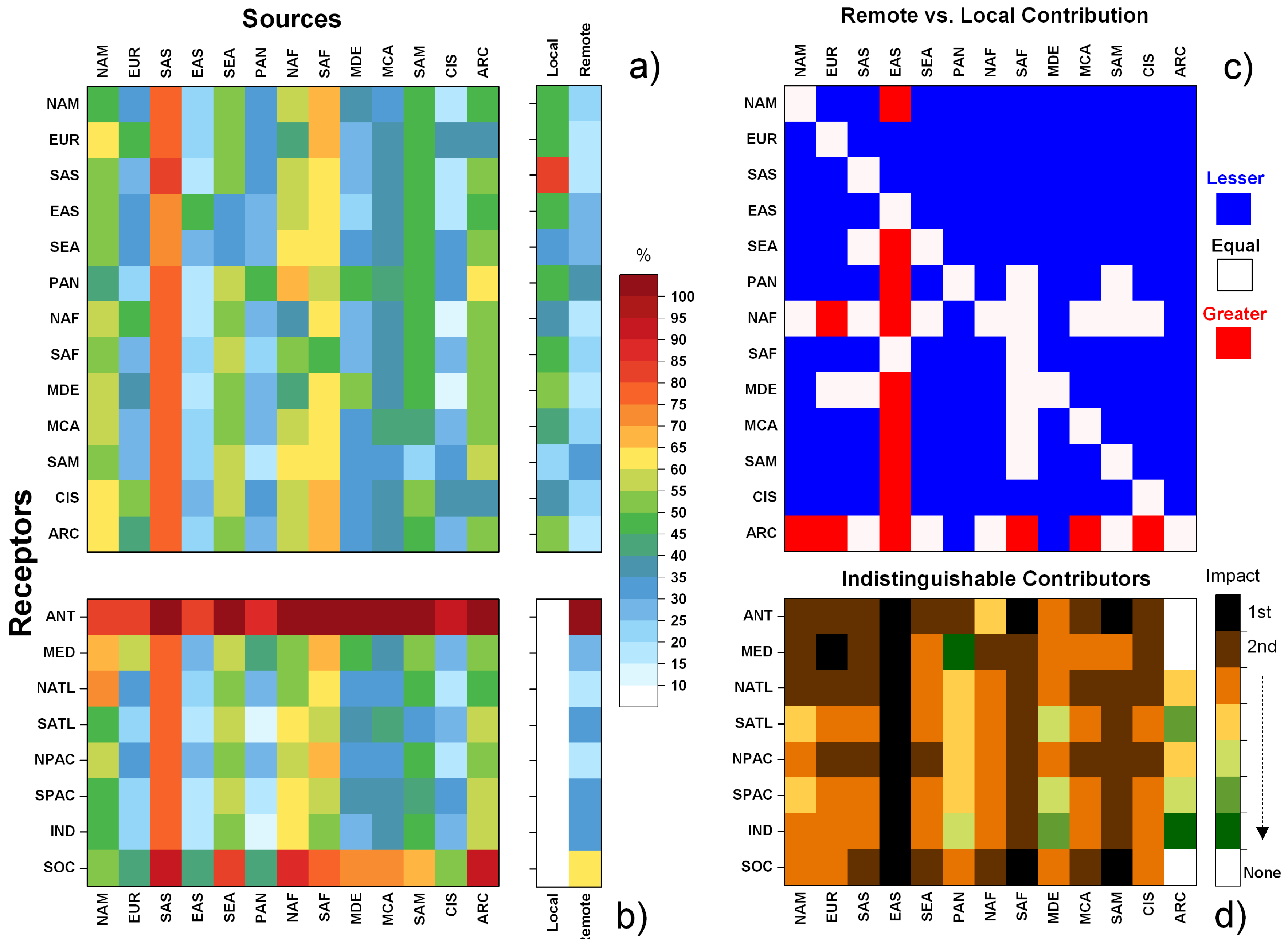
| NAM | EUR | SAS | EAS | SEA | PAN | NAF | SAF | MDE | MCA | SAM | CIS | ARC | REMOTE | ALL-Sources | |
|---|---|---|---|---|---|---|---|---|---|---|---|---|---|---|---|
| Deposition to Lands | |||||||||||||||
| NAM | 17.1 | 4.7 | 3.9 | 29.3 | 3.2 | 0.3 | 1.7 | 5.3 | 0.7 | 4.1 | 3.2 | 4.7 | 0.3 | 61.7 | 383.7 |
| (13.2–21.5) | (4.2–5.6) | (2.2–5.2) | (26.5–33.5) | (2.2–4.0) | (0.2–0.3) | (1.1–2.1) | (3.3–6.8) | (0.6–0.8) | (3.4–4.6) | (2.2–3.8) | (4.2–5.0) | (0.2–0.4) | (54.0–66.9) | (369.5–398.9) | |
| EUR | 1.4 | 18.4 | 1.1 | 8 | 0.9 | 0.1 | 0.6 | 1.5 | 0.3 | 1 | 0.9 | 2.3 | 0.1 | 18.1 | 129.2 |
| (1.0–1.9) | (14.0–23.1) | (0.6–1.4) | (7.3–8.9) | (0.6–1.1) | (0.1–0.1) | (0.5–0.7) | (0.9–1.9) | (0.2–0.3) | (0.8–1.1) | (0.6–1.1) | (2.0–2.8) | (0.1–0.1) | (16.1–19.4) | (118.8–140.4) | |
| SAS | 0.8 | 1.3 | 18.2 | 7.9 | 1.3 | 0.1 | 0.6 | 2.1 | 0.5 | 1.2 | 1.3 | 1.4 | 0.1 | 18.8 | 150.4 |
| (0.6–1.0) | (1.2–1.5) | (10.7–25.3) | (7.2–8.8) | (0.9–1.6) | (0.1–0.1) | (0.4–0.8) | (1.4–2.7) | (0.4–0.5) | (1.0–1.4) | (1.0–1.6) | (1.3–1.5) | (0.0–0.1) | (16.6–20.4) | (138.7–161.9) | |
| EAS | 2.6 | 4.5 | 7.2 | 104.1 | 4.5 | 0.3 | 1.6 | 5.3 | 0.8 | 3.2 | 3.2 | 5.5 | 0.2 | 39 | 445.0 |
| (2.0–3.4) | (4.0–5.5) | (4.2–9.5) | (82.9–134.5) | (3.7–5.1) | (0.2–0.3) | (1.1–2.0) | (3.3–6.7) | (0.7–0.9) | (2.5–3.7) | (2.3–3.9) | (5.0–6.1) | (0.2–0.3) | (32.3–44.0) | (399.8–499.9) | |
| SEA | 0.6 | 0.9 | 2.6 | 7.5 | 3.5 | 0.2 | 0.5 | 2.1 | 0.2 | 1.2 | 1.4 | 0.9 | 0.1 | 18.2 | 118.4 |
| (0.4–0.7) | (0.8–1.1) | (1.5–3.4) | (6.6–8.6) | (2.9–4.1) | (0.1–0.2) | (0.4–0.7) | (1.4–2.7) | (0.2–0.2) | (0.9–1.4) | (1.1–1.7) | (0.7–1.0) | (0.0–0.1) | (15.4–20.4) | (103.2–127.9) | |
| PAN | 0.3 | 0.5 | 0.7 | 3.6 | 1.1 | 2.1 | 0.4 | 2.6 | 0.1 | 1 | 2 | 0.5 | 0 | 12.9 | 111.8 |
| (0.3–0.4) | (0.5–0.6) | (0.4–0.9) | (3.3–3.9) | (0.7–1.4) | (1.6–2.6) | (0.3–0.6) | (1.8–3.3) | (0.1–0.1) | (0.8–1.2) | (1.5–2.4) | (0.4–0.6) | (0.0–0.0) | (10.4–15.1) | (107.0–115.4) | |
| NAF | 2 | 5.5 | 2.3 | 14.8 | 1.8 | 0.2 | 2.3 | 3.6 | 0.6 | 2 | 1.9 | 2.5 | 0.1 | 37.5 | 231.8 |
| (1.5–2.7) | (4.5–7.2) | (1.3–3.0) | (13.5–16.3) | (1.3–2.3) | (0.1–0.2) | (1.8–2.7) | (2.3–4.6) | (0.5–0.7) | (1.6–2.3) | (1.4–2.3) | (2.3–2.6) | (0.1–0.2) | (33.7–39.7) | (218.2–242.8) | |
| SAF | 2.1 | 3.8 | 4.8 | 22.1 | 4.5 | 0.6 | 2.7 | 22.9 | 0.9 | 4.3 | 6.5 | 3.2 | 0.2 | 55.8 | 456.5 |
| (1.7–2.8) | (3.3–4.3) | (2.7–6.4) | (19.9–24.3) | (3.1–5.6) | (0.6–0.7) | (1.9–3.3) | (17.2–27.9) | (0.–1.0) | (3.4–5.0) | (4.8–7.7) | (2.7–3.6) | (0.1–0.2) | (48.4–61.9) | (417.5–486.5) | |
| MDE | 0.7 | 1.6 | 1.1 | 5.9 | 0.8 | 0.1 | 0.5 | 1.4 | 1.7 | 0.8 | 0.8 | 1.1 | 0.1 | 14.9 | 95.0 |
| (0.5–0.9) | (1.4–2.0) | (0.6–1.4) | (5.4–6.5) | (0.5–1.0) | (0.1–0.1) | (0.4–0.6) | (0.9–1.8) | (1.3–2.2) | (0.7–1.0) | (0.6–1.0) | (1.0–1.2) | (0.0–0.1) | (13.2–16.0) | (91.0–98.5) | |
| MCA | 1.1 | 1.2 | 1.2 | 7.5 | 1.1 | 0.1 | 0.7 | 2.3 | 0.2 | 3.3 | 1.3 | 1.1 | 0.1 | 17.9 | 124.2 |
| (0.8–1.4) | (1.0–1.4) | (0.7–1.6) | (6.7–8.3) | (0.7–1.3) | (0.1–0.1) | (0.4–0.8) | (1.5–3.0) | (0.2–0.2) | (2.7–4.1) | (1.0–1.6) | (0.9–1.2) | (0.0–0.1) | (15.5–19.7) | (112.1–132.6) | |
| SAM | 1.5 | 2.5 | 3.1 | 16.2 | 3.6 | 0.7 | 2 | 9.3 | 0.5 | 4.1 | 12.3 | 2.3 | 0.1 | 46 | 386.6 |
| (1.2–2.0) | (2.2–2.9) | (1.7–4.1) | (14.4–17.9) | (2.5–4.5) | (0.6–0.7) | (1.3–2.6) | (6.1–11.7) | (0.4–0.6) | (3.3–4.7) | (10.5–13.6) | (1.9–2.6) | (0.1–0.2) | (38.4–52.6) | (349.7–411.8) | |
| CIS | 3.6 | 10.1 | 3.2 | 27.2 | 2.7 | 0.2 | 1.5 | 4.4 | 0.8 | 2.9 | 2.6 | 19.5 | 0.6 | 60 | 355.6 |
| (2.7–4.9) | (8.1–13.4) | (1.8–4.3) | (24.2–31.7) | (1.9–3.4) | (0.2–0.3) | (1.0–1.9) | (2.7–5.6) | (0.6–0.9) | (2.3–3.4) | (1.9–3.2) | (15.7–23.1) | (0.5–0.7) | (53.6–66.2) | (333.4–380.3) | |
| ARC | 2.2 | 3.9 | 1.8 | 14.9 | 1.5 | 0.1 | 0.8 | 2.5 | 0.4 | 1.6 | 1.5 | 3.7 | 0.9 | 35.1 | 154.0 |
| (1.6–3.0) | (3.3–5.0) | (1.0–2.4) | (13.5–16.9) | (1.1–1.9) | (0.1–0.1) | (0.6–1.0) | (1.5–3.1) | (0.3–0.4) | (1.3–1.9) | (1.1–1.8) | (3.3–4.3) | (0.6–1.1) | (31.9–37.8) | (144.3–168.1) | |
| ANT | 0.1 | 0.2 | 0.3 | 1.4 | 0.4 | 0.2 | 0.2 | 1.1 | 0 | 0.4 | 1 | 0.2 | 0 | 5.5 | 52.4 |
| (0.1–0.2) | (0.1– 0.3) | (0.1–0.5) | (1.0–2.1) | (0.2–0.8) | (0.1–0.2) | (0.1–0.4) | (0.6–2.0) | (0.0–0.1) | (0.2–0.7) | (0.5–1.6) | (0.1–0.3) | (0.0–0.0) | (3.3–9.2) | (36.5–82.7) | |
| Deposition to Basins | |||||||||||||||
| MED | 0.4 | 3.2 | 0.4 | 2.6 | 0.3 | 0 | 0.4 | 0.5 | 0.1 | 0.3 | 0.3 | 0.6 | 0 | 9.2 | 41.9; |
| (0.3–0.6) | (2.4–4.3) | (0.2–0.5) | (2.3–3.0) | (0.2–0.4) | (0.0–0.0) | (0.3–0.5) | (0.3–0.7) | (0.1–0.2) | (0.3–0.4) | (0.2–0.4) | (0.5–0.7) | (0.0–0.0) | (8.0–10.5) | (38.2–45.9) | |
| NATL | 14.5 | 13 | 8.9 | 60.9 | 7.7 | 0.8 | 4.6 | 15.4 | 1.6 | 9 | 8.7 | 9.4 | 0.6 | 155.8 | 843.6 |
| (10.3–20.8) | (11.5–15.7) | (5.0–11.9) | (55.4–67.9) | (5.3–9.5) | (0.6–0.9) | (3.2–5.6) | (9.6–19.4) | (1.3–1.8) | (7.3–10.3) | (6.2–10.4) | (8.5–10.1) | (0.5–0.8) | (140.2–165.2) | (814.6–865.3) | |
| SATL | 2.5 | 4.1 | 5.4 | 27.7 | 7.3 | 2 | 3.6 | 19.8 | 0.9 | 7.3 | 16.3 | 3.9 | 0.3 | 101.1 | 760.3 |
| (2.0–3.2) | (3.7–4.6) | (3.0–7.2) | (25.2–29.7) | (5.0–9.2) | (1.9–2.1) | (2.3–4.6) | (13.2–24.5) | (0.7–1.0) | (5.7–8.7) | (13.3–18.7) | (3.3–4.4) | (0.2–0.3) | (83.5–115.4) | (725.3–790.1) | |
| NPAC | 16.7 | 26.6 | 26.9 | 200.4 | 24.2 | 2.3 | 11.5 | 39.9 | 4.4 | 26.4 | 25.9 | 26.5 | 1.6 | 436.3 | 2400.8 |
| (13.1–22.3) | (23.4–31.7) | (15.0–35.7) | (179.5–237.0) | (17.0–29.8) | (1.9–2.5) | (7.8–14.5) | (24.6–50.7) | (3.6–5.1) | (21.3–30.0) | (18.5–31.1) | (24.3–28.5) | (1.1–2.0) | (388.8–467.0) | (2309.8–2471.7) | |
| SPAC | 6.6 | 10.7 | 13.1 | 72.2 | 19.5 | 6.6 | 8.3 | 43.8 | 2.2 | 20.8 | 36.2 | 10.1 | 0.7 | 251.4 | 1869.1 |
| (5.3–8.4) | (9.5–12.1) | (7.3–17.7) | (65.5–78.6) | (13.2–24.2) | (6.2–7.3) | (5.3–10.6) | (28.5–54.3) | (1.7–2.5) | (16.6–24.0) | (26.8–42.7) | (8.5–11.6) | (0.5–0.9) | (208.1–285.2) | (1786.3–1945.5) | |
| IND | 4.5 | 7.4 | 16.5 | 51.9 | 14.1 | 2.7 | 5.4 | 31.6 | 1.8 | 11.6 | 20.4 | 7.1 | 0.5 | 176 | 1208.0 |
| (3.7–5.8) | (6.6–8.4) | (9.3–21.8) | (47.1–56.5) | (9.9–17.3) | (2.5–2.8) | (3.5–6.9) | (22.5–38.4) | (1.5–2.1) | (9.2–13.5) | (14.9–24.1) | (6.0–8.1) | (0.3–0.6) | (145.3–199.2) | (1156.5–1254.8) | |
| SOC | 0.3 | 0.4 | 0.6 | 3 | 0.9 | 0.3 | 0.4 | 2.3 | 0.1 | 0.9 | 2 | 0.4 | 0 | 11.5 | 88.2 |
| (0.2–0.3) | (0.4–0.5) | (0.3–0.9) | (2.5–3.7) | (0.6–1.3) | (0.3–0.4) | (0.2–0.6) | (1.5–3.3) | (0.1–0.1) | (0.6–1.2) | (1.4–2.7) | (0.3–0.5) | (0.0–0.0) | (8.6–15.7) | (70.6–120.7) | |
© 2017 by the authors. Licensee MDPI, Basel, Switzerland. This article is an open access article distributed under the terms and conditions of the Creative Commons Attribution (CC BY) license (http://creativecommons.org/licenses/by/4.0/).
Share and Cite
De Simone, F.; Hedgecock, I.M.; Carbone, F.; Cinnirella, S.; Sprovieri, F.; Pirrone, N. Estimating Uncertainty in Global Mercury Emission Source and Deposition Receptor Relationships. Atmosphere 2017, 8, 236. https://doi.org/10.3390/atmos8120236
De Simone F, Hedgecock IM, Carbone F, Cinnirella S, Sprovieri F, Pirrone N. Estimating Uncertainty in Global Mercury Emission Source and Deposition Receptor Relationships. Atmosphere. 2017; 8(12):236. https://doi.org/10.3390/atmos8120236
Chicago/Turabian StyleDe Simone, Francesco, Ian M. Hedgecock, Francesco Carbone, Sergio Cinnirella, Francesca Sprovieri, and Nicola Pirrone. 2017. "Estimating Uncertainty in Global Mercury Emission Source and Deposition Receptor Relationships" Atmosphere 8, no. 12: 236. https://doi.org/10.3390/atmos8120236