Integrated Regional Enstrophy and Block Intensity as a Measure of Kolmogorov Entropy
by
 , and
, and
Andrew D. Jensen
1, 
Anthony R. Lupo
2,3,*,
Igor I. Mokhov
4,5,
Mirseid G. Akperov
4 and
DeVondria D. Reynolds
2 1
Department of Mathematics and Meteorology, Northland College, Ashland, WI 54806, USA
2
Atmospheric Science Program, School of Natural Resources, University of Missouri, Columbia, MO 65211, USA
3
Department of Natural Resources Management and Land Cadastre, Belgorod State University, Belgorod 308015, Russia
4
A.M.Obukhov Institute of Atmospheric Physics, Russian Academy of Sciences, 3 Pyzhevsky per, Moscow 119017, Russia
5
Department of Physics, Lomonosov Moscow State University, Moscow 119991, Russia
*
Author to whom correspondence should be addressed.
Atmosphere 2017, 8(12), 237; https://doi.org/10.3390/atmos8120237
Submission received: 2 October 2017
/
Revised: 27 October 2017
/
Accepted: 21 November 2017
/
Published: 29 November 2017
(This article belongs to the Section Meteorology)
Abstract
:Enstrophy in a fluid relates to the dissipation tendency in a fluid that has use in studying turbulent flows. It also corresponds to vorticity as kinetic energy does to velocity. Earlier work showed that the integrated regional enstrophy (IRE) was related to the sum of the positive Lyapunov exponents. Lyapunov exponents are the characteristic exponent(s) of a dynamic system or a measure of the divergence or convergence of system trajectories that are initially close together. Relatively high values of IRE derived from an atmospheric flow field in the study of atmospheric blocking was identified with the onset or demise of blocking events, but also transitions of the large-scale flow in general. Kolmogorv–Sinai Entropy (KSE), also known as metric entropy, is related to the sum of the positive Lyapunov exponents as well. This quantity can be thought of as a measure of predictability (higher values, less predictability) and will be non-zero for a chaotic system. Thus, the measure of IRE is related to KSE as well. This study will show that relatively low (high) values of IRE derived from atmospheric flows correspond to a more stable (transitioning) large-scale flow with a greater (lesser) degree of predictability and KSE. The transition is least predictable and should be associated with higher IRE and KSE.
1. Introduction
Blocking can be described generically as a persistent large-scale mid-latitude positive geopotential height anomaly (e.g., [1]). About the same time, Dymnikov et al. [2] described blocking as a meridional perturbation that destabilizes the zonal flow. This work [2], derived a quantity called integrated regional enstrophy (IRE), which can be used as a measure for change in the zonal flow that may indicate onset or decay blocking [3,4]. The quantity of IRE conjectures that the blocking domain sum of the flow enstrophy is related to the sum of the positive eigenvalues of the linearization operator of the barotropic vorticity equation [2,3,4]. As such, IRE can also be regarded as a flow stability indicator [3,4,5]. The work of [3] demonstrated for three case studies of Southern Hemisphere blocking, that IRE increased locally with the decay of each blocking event, and was relatively low during the maintenance period. This study and those of [6,7] suggest blocking does not survive the transition of large-scale flow regimes. The work of [4] examined more than 100 cases of northern hemisphere blocking over a three-year period and found that local increases in IRE can be associated with the onset or termination of blocking.
Later, this quantity was used to examine the dynamics of the blocking episode associated with the Russian heat wave and drought of summer 2010 [8]. The blocking episode involved four individual strong and persistent blocking events from 1 May to 16 August 2010 over Russia and Eastern Europe which contributed to the drought conditions [8,9,10,11]. The onset and decay of each blocking case with local maxima in the IRE as was shown by [3,4], who seemed to indicate this quantity was a reliable indicator of blocking. However, Jensen et al. [5,12] showed that IRE would identify flow regime transitions in general, whether there was blocking present or not. Then Jensen et al. [12] examined a persistent and strong Pacific Region case during January and February 2014, and demonstrated that this event survived the transition between one phase and another in the Pacific North American (PNA) pattern due to the fortuitous timing of synoptic-scale forcing [13].
Enstrophy in a geophysical fluid relates to the dissipation tendency, and this quantity has use in studying turbulent flows (e.g., [14,15,16,17]). Many studies have shown that IRE is related to the sum of the positive Lyapunov exponents as discussed first by [2] and later by the work cited above and by [12] flow stability. Lyapunov exponents are the characteristic exponent(s) of a dynamic system or a measure of the divergence or convergence of system trajectories that are initially close together, in this case two similar atmospheric states (e.g., [18]). Although relatively high values of IRE derived from an atmospheric flow field in the study of atmospheric blocking were identified with the onset or demise of blocking events, IRE can also be associated with transitions of the large-scale flow in general, and thus are not exclusive to blocking [12]. Recently [19], however, used covariant Lyapunov vectors to identify blocking flows in a simple channel model with orography. As stated in [19], each covariant Lyapunov vector is associated with a Lyapunov exponent, representing the growth or decay rates in blocked or zonal flows. They found growth rates corresponding to more unstable flow during blocked flows.
Recently, Lupo et al. [14] studied the nature of predictability in a blocking event using a relationship developed by [15]. The authors in [15] related the Reynolds number in a fluid flow to the Lyapunov exponent of the Navier–Stokes equation for large Reynolds number flows, and this can be associated with the characteristic growth rate of the disturbances in the flow. For more details on the derivation, see [14,15]. They argued that if the growth rate associated with the Reynolds number is larger than that implied by the Lyapunov exponent, the flow can be characterized as ‘roughly dependent on initial conditions’, as opposed to sensitive dependence on initial conditions, in which the Reynolds number growth rate is less than or equal to the Lyapunov exponent. Then, since IRE is related to the Lyapunov exponent, Lupo et al. [14] related IRE to the Reynolds number growth rate and showed that for a blocking event, the IRE was similar in magnitude to this growth rate. Thus, large-scale events like blocking would be sensitively dependent on initial conditions.
Kolmogorov (Kolmogorov–Sinai) entropy (abbreviated here as KSE), also known as metric entropy, is related to the sum of the positive Lyapunov exponents as well through Pesin theory (e.g., [16,17,20,21,22]). This quantity can be thought of as a measure of predictability (higher values, less predictability) and will be non-zero for a chaotic system. One goal of this work will be to demonstrate that KSE and IRE can be related. Other investigators (e.g., [23]), have also used KSE to study the stability and predictability found in atmospheric flows.
The block intensity (BI) is a quantity first proposed by [1], which is calculated as the mean lifetime value of the daily normalized central height values of the event. The normalization is proportional to the upstream and downstream height gradients, and Wiedenmann et al. [24] modified and standardized the estimate of the gradients. They [24] also demonstrated that BI increased nearly linearly with increases in the upstream and downstream height gradient, and thus had use as a flow regime blocking diagnostic. The second goal of this work is to demonstrate that IRE, KSE, and BI all show similar behavior over the lifetime of two blocking events. These case studies have been examined previously in order that comparisons can be made to prior findings. Section two will describe the data and methods used. Section three will describe the cases and analyze them, and section four will highlight the main conclusions of this work.
2. Data and Methods
2.1. Data
In order to meet our objective, the National Centers for Environmental Prediction/National Center for Atmospheric Research (NCEP/NCAR) re-analyses [25], archived at the NCAR research facilities in Boulder, CO [26], were used, which provide for large-scale meteorological data at various resolutions from 1° × 1° to 2.5° × 2.5° latitude–longitude grids. We will use the 500 hPa height data (m) available at 1200 UTC daily, since these contain the most observational data.
2.2. Methods
Here we use the work of [2], who postulated that if the atmosphere is barotropic, the positive Lyapunov exponent(s) in the atmosphere can be expressed as the area of integrated regional enstrophy (IRE):
where λi is the ith Lyapunov exponent that is greater than zero in a dynamic system, ζ is the vorticity, or the curl of the wind vector, and the quantity squared is called enstrophy, which is the dissipation tendency of a fluid. A constant proportional to unity is implied by the very high correlation [2]. Many studies (e.g., [3,4,8,9,12,13]), have demonstrated the utility of IRE in identifying the onset and termination of atmospheric blocking and flow regime transformation. In (1), the vorticity is calculated via the geostrophic relationship using second order finite differencing and IRE is calculated over the blocking region (40° latitude by 60° longitude) following [4,8].
As the sum of the positive Lyapunov exponents, IRE relates to predictability and can be also related to the production of system information, e.g., KSE (Kolmogorov–Sinai Entropy or metric entropy) (e.g., [15,16]). In theory, the larger the IRE, the less predictable the atmosphere is, as trajectories of two initial conditions could diverge very rapidly with time (e.g., [14]). Then, relatively low (high) values of IRE derived from atmospheric flows may correspond to more stable (transitioning) large-scale flows with a greater (lesser) degree of predictability and KSE. The flow regime transition period should be the least predictable and should be associated with higher IRE and KSE.
Then, the work of [16] discussed KSE as the mean rate of system information production through the concept of sensitive dependence on initial conditions, which is a characteristic of a system that displays chaos. In such a system where time is continuous, the Lyapunov exponents are defined using Oseledets theorem [20]:
Here the subscript represents the ith characteristic exponent in an n-dimensional system, and ε(0) represents the initial separation of trajectories that are infinitesimally close, and εi(t) represents their separation at time t. The Lyapunov exponents (λi) measure the expansion (contraction) of an infinitesimally small n-dimensional sphere at the initial condition, becoming an n-dimensional ellipsoid in the phase space flow. It follows that εi(t) is the length of the ith principal axis of the ellipsoid and a positive (negative) Lyapunov exponent represents trajectory divergence (convergence) in the phase space. Additionally, Ekmann et al. [16] argued that in (2), the system entropy (or KSE), and Hausdorff (fractal) dimension are all related to the degree to which a system can be described as chaotic. Further, Ekmann et al. [16] argued that KSE is bounded in terms of the Lyapunov exponents and using Ruelle’s Therorem [21] we can write:
where λi are the positive Lyapunov exponents. In (3), the subscript represents only those Lyapunov exponents greater than zero. Then, the equality from (3) holds often (not always) for physical measures such as entropy or KSE [16] as proposed by Pesin’s theorem [22]. This theorem implies that KSE can be written as:
and (4) is referred to as the Pesin identity or ‘correlation’ entropy [16], which is the lower bound of the KSE [16].
Here, the value of (4) was calculated using the nonlinear time series analysis R-package. In order to calculate the KSE, we must first calculate the correlation dimension, which is a standard measure of the dimensionality of a set of points (i.e., a time series). Let be the points of a time series. Following [16], we consider the functions , and , where is Euclidean distance or some other norm, is the embedding dimension, and is a tolerance. The method used here reconstructs the dynamics of the time series (here potential vorticity) by embedding it in a higher dimension called the embedding dimension . In order to calculate the KSE, the algorithm estimates the embedding dimension between two bounds. For our examples, we chose to calculate the KSE by estimating the embedding dimension to be between two and 10. Similar results to those reported here were obtained by lowering the upper estimated embedding dimension. The correlation dimension is estimated by plotting log vs. and using linear regression to calculate the slope. The result is then used to estimate the KSE by calculating . In order to achieve a time series of sufficient length, we used 11 days for the mid-life intensification and 21 and 24 d for each blocking event, and the output was a single value or point estimate representing this time period. The KSE was calculated with both six-hourly and daily data and the results compared. Both resulted in similar values of the KSE.
Thus, it is trivial to demonstrate that the KSE can be represented formally in terms of Equation (1) to get:
The relationship above is suggested by the relationship between IRE, the sum of the positive local Lyapunov exponents, and Equation (4). We note that the relationship indicated by (~) is purely formal and is not meant to indicate a rigorous mathematical approximation with error estimates. The calculations below provide further evidence that the relationship suggested above is useful.
One of the blocking events studied here onset at 0000 UTC 23 January 2014, and terminated at 0000 16 February 2014, and was studied in [13]. The other event occurred in a similar area and onset 0000 UTC 23 February 2017 and terminated at 0000 UTC 16 March These events and all Northern hemisphere events occurring since July 1968 can be found on the University of Missouri Blocking Archive [27]. During the block lifetime, the block intensity was calculated daily for this event at 1200 UTC from onset to termination, following [24] and the formula for intensity is given by Equation (6):
where Zm is the central height value (m) for the blocking event at 1200 UTC and RC is the mean contour representing the upstream and downstream gradients calculated using;
where Zu and Zd are the lowest (trough axis) heights upstream and downstream of the block. The resultant value of BI is a diagnostic quantity. For more details regarding this calculation, see [1] or [24]. Thus, the normalization value represents a one-pass Shapiro-type filter [28] on the wave length of twice the grid-scale (approximately 400 km at 45° N) or the synoptic and large-scale scale component of the flow. Then, BI can be thought of as the normalized central height maximum or relative strength of the sub-synoptic-scale component of the flow. The mean BI for the Northern Hemisphere since July 1968 is 3.11, and the distribution of BI is Gaussian [1,24]. These studies define a strong (weak) blocking event as an event that is one standard deviation greater (less) than these values, and [24] defines a weak blocking event as having a BI less than 2.0 and a strong blocking event as one with a BI greater than 4.3. Similar bounds for values of KSE and IRE have not been explored, since these quantities can be determined for any flow regime and not just blocking such as BI.
3. Results—Blocking Case Studies
3.1. Blocking Case: January–February 2014
The blocking event examined here occurred during 23 January to 16 February 2014 and was located over the Eastern Pacific near the Gulf of Alaska and near the West Coast of North America (130° W). This event formed out of a very long-lived ridge over the same area associated with an area of warm SST referred to colloquially as ‘the blob’ (e.g., [13,29,30,31]). This event dominated a significant period of the winter season, and was likely to be at least partly responsible for the cold winter over North America that year (e.g., [13,32]). The work of [13] describes this event in more detail and [31] used non-equilibrium thermodynamics following [33] and references therein to show that this event was associated with entropy production in the free atmosphere and at the surface in the region of the event during January and February of that year. Then, Jensen et al. [13] demonstrated that the 500 hPa height field evolved during the intensification stage of the blocking event, as shown in Figure 1. This event was noteworthy as it survived a large-scale flow regime change during early February 2014 (4th–7th), as the Pacific North American (PNA) teleconnection pattern changed from positive to negative during early February 2014 [34]. The PNA index (see [34]—available from [26,34]) from 21 to 31 January 2014 was 0.511, and from 1 to 16 February was −0.823. Earlier work (e.g., [3,6]) has suggested that blocking events would not survive a transition in the large-scale flow regime. Additionally, this event is noteworthy for the intensity (BI = 5.93) and persistence (24 d) [27], and Jensen et al. [13] described the event as one of the 15 strongest events persisting for more than 20 d over the entire period of record.
3.2. Blocking Case: February–March 2017
Another strong Pacific blocking event (BI = 4.51, Figure 2a) was first identified on 0000 UTC 23 February 2017 near 50° N 160° W within the Bering Sea region in the eastern Pacific. The event persisted for 21 days and remained relatively stationary before decay and the event terminated near the international dateline on 0000 UTC 16 March 2017. On 4 March 2017, a separate event developed over the Atlantic region, which means that the Northern Hemisphere experienced simultaneous blocking (not shown). The Atlantic event was also strong and the observation that both simultaneously occurring blocking events tend to be strong was shown by [24]. Unlike the 2014 event described above, this event persisted in a negative PNA environment (mean PNA index = −0.669) and underwent decay as the PNA transitioned to the positive phase. This event was studied initially in order to test the ability of an ensemble model to forecast the onset of the event up to seven days in advance [35]. This pilot study [35] showed that the event was forecast only up to four days in advance by an ensemble model, but the intensity and duration of the event were under forecast as most previous blocking studies suggest (e.g., [11]). For this event, there was a mid-lifecycle peak in intensity that was associated with a strong upstream cyclone development, and the onset of the Atlantic event described above.
3.3. Blocking Cases: BI, IRE, KSE
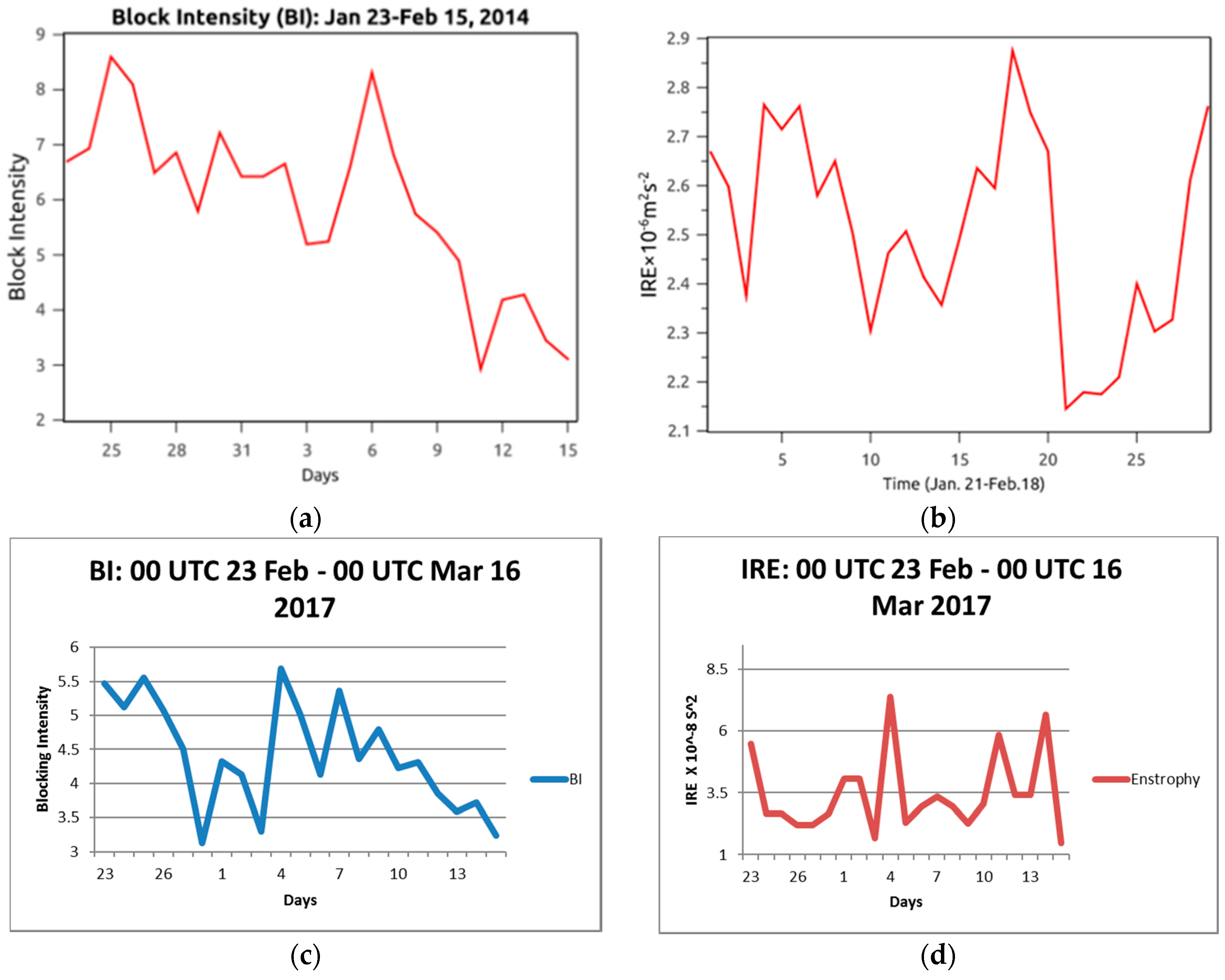
Examining the block intensity (BI) [24] for both cases (Figure 3a,c) demonstrates that each blocking event was most intense just following the onset of the event. The winter 2014 event intensified again in early February (3rd–6th) near the same time that the phase of the PNA changed from positive to negative indicating flow regime change [34]. The winter 2017 event underwent intensification in early March (2nd–7th). The work of [1] demonstrated the connection between block onset and cyclogenesis, and then [36] demonstrated that rapid height rises, and thus BI, follows upstream cyclogenesis during onset and mid-life block intensification. In the case of the first event, BI was markedly less after the PNA transition, indicating a weaker block until the decay period and termination. For the second event, the BI trended downward following 7 March 2017, reaching the minimum value (BI = 3.24) at termination. The IRE diagnostic also followed a similar evolution during the lifecycle of both events (Figure 3b,d), with the IRE reaching local maxima during onset, intensification, and termination.
Note that during the onset and mid-life intensification periods of the winter 2014 case (Table 1), both the BI and IRE were greater than the mean of the block lifecycle. The correlation coefficient between the two time-series was 0.45, which is significant at the 95% confidence level. The calculation for the correlation coefficient and the significance can be found in any introductory statistics text (e.g., [37]). However, if BI is lagged by 24 h, testing the assertion of [35,36], the correlation is 0.72, which is significant at the 99% confidence level supporting the possible lag relationship suggested by [35,36]. For the winter 2017 blocking case (Table 2), BI was relatively high for both the onset and intensification period, however, IRE did not increase markedly for 72 h following onset. The correlation coefficient between BI and IRE for this event was only 0.25 for the entire event (not quite significant at the 90% level), but when the BI was lagged by 72-h as suggested above the correlation coefficient was 0.45, significant at the 95% confidence level. Further time lags resulted in a decrease in correlation between BI and IRE for both events.
This lag between IRE and BI was studied in [35]. The work of [36] (and references therein) suggested that upstream cyclogenesis is a necessary condition for block onset or block intensification during the mid-block period. They also showed that the central height value and, thus, BI continues to increase for a short period following upstream cyclogenesis. Then, the pilot study of [35] suggested that first cyclogenesis occurs and then IRE increases, followed by BI for four case studies, including the winter 2017 case here. Additionally, in order to attempt to explain the difference in the lag times for each case, the deepening rates of the upstream cyclones were calculated. For the winter 2014 event, the upstream cyclone deepened from 983 hPa to 956 hPa near 40° N from 0000 UTC 20 to 0000 UTC 21 January 2014. This is a deepening rate of 1.5 Bergerons according to the criterion for explosive cyclogenesis published in [38]. The deepening rate of the cyclone preceding the winter 2017 event was only 1.0 Bergerons, as it deepened from 997 hPa to 977 hPa from 0000 UTC 20 to 0000 UTC 21 February 2017 at 45° N. Thus, the stronger deepening rate of the winter 2014 event might partly explain the smaller lag time between IRE and BI. However, more case studies would need to be examined in order to support the conclusions stated in this paragraph, and this analysis is the subject of another study [35].
In order to examine the relationship between IRE, BI, and KSE, the mid-lifecycle intensification periods will be examined here. IRE and KSE can be calculated for any mid-latitude flow, but BI can only be calculated while a block is present. Due to the algorithm used to calculate KSE, daily values could not be computed. Table 1 and Table 2 show that the KSE was relatively high during the mid-life intensification periods when compared to the value calculated over the entire block lifecycle from onset to termination. The results of Table 1 in combination with the higher correlations between BI and IRE suggest a correlation between all three quantities during the block lifecycle. For the winter 2104 event the mid-block intensification period was 11 days for all three variables (30 January–9 February 2014), even though intensification occurred over the shorter period of 2–7 February 2014. The mid-block intensification period for the winter 2017 blocking event was 2–7 March 2017. Thus, the 11-day calculation periods for the KSE included a decline in the values of BI and IRE. The onset intensification period calculation for both events were of different lengths, as noted in Table 1 and Table 2, but the results of this period generally support the position here that all three variables are generally larger during mid-life intensification for both events than for the entire block life cycle. However, due to the length of the time series used for KSE, the calculation included a significant part of the pre-block time period and may not represent the early intensification at all. Rather this quantity may indicate the pre-block conditions here.
4. Discussion, Summary and Conclusions
The objectives of this study were to determine whether IRE and KSE are similar quantities mathematically, and whether IRE, KSE, and BI provide the same information about the dynamics of blocking. A very strong blocking event that occurred in the Pacific Ocean Basin during the winter of 2013–2014 and another strong event occurring over the same region during February and March 2017 were selected for study to demonstrate the utility of the methods provided here, and to compare with other recent publications which examined these events [13,32,35]. The first objective was met in section two by describing the development of KSE and comparing expressions of IRE and KSE.
Blocking can develop very rapidly and models often fail to anticipate its onset and/or decay, especially decay after about ten days [39]. These results corroborate such studies and suggests that the predictability of the mid-block intensification periods would have been low after the onset period, and similar to [35,39], predict that the approximate decay period for both events could only be achieved with low confidence. Since blocking is maintained by vigorously developing, upstream, synoptic-scale, extratropical cyclones during the block lifecycle ([1,35,36] and many others), the time-scale for predictability of the onset, mid-life intensification, and decay of blocking may be limited to that of synoptic-scale cyclones. This may be an inherent characteristic of blocking, which indicates that we can expect limited progress in blocking predictability based on today’s understanding of these events as well as the modeling currently available to the community.
The results of [14] (and others) demonstrated that while predictability for blocking may be difficult, it is not impossible in a general sense. However, the timing of onset, intensification and decay will be governed by synoptic-scale processes [35,36]. Additionally, Schubert et al. [19] suggested that blocked flows were identifiable using Lyapunov exponents and are more unstable and more difficult to predict in their simplified model. This agrees with [2,12], and the results found here show that the Lyapunov exponents were relatively high at onset and intensification. Here we did not compare the values of IRE or KSE during blocked and non-blocked flow since BI cannot be calculated during non-blocked flows.
The work here also demonstrated that for these blocking events, IRE, KSE, and BI are all relatively large during the mid-block intensification, and suggest similar behavior at block onset. This indicates that each quantity represents a similar dynamic character for the large-scale flow during the life-cycle of this blocking event. Also, the correlation coefficient between BI and IRE, which was even stronger when BI lagged IRE by 24 h for the first event and 72 h for the second event, supports the earlier works of [35,36] on the relationship between upstream cyclogenesis and block development and intensification. The next step in this research will be to study several blocking events [35] and examine the behavior of BI, IRE, and KSE, as well as evaluating the ability of numerical models to capture the evolution of these three quantities during a forecast period of block onset or some other period within the block lifecycle.
Acknowledgments
The authors would like to acknowledge the anonymous reviewers of this work. Their time and effort made this a stronger contribution to the literature. Igor I. Mokhov and Mirseid G. Akperov were supported by the Russian Ministry of Education and Science, agreement Nº 14.616.21.0082 (RFMEFI61617X0082).
Author Contributions
Anthony R. Lupo and Andrew D. Jensen conceived and designed the experiments; Andrew D. Jensen and DeVondria D. Reynolds performed the experiments; all five authors analyzed the data and wrote the paper.
Conflicts of Interest
The authors declare no conflict of interest.
References
- Lupo, A.R.; Smith, P.J. Climatological features of blocking anticyclones in the Northern Hemisphere. Tellus Ser. A 1995, 47, 439–456. [Google Scholar] [CrossRef]
- Dymnikov, V.P.; Kazantsev, Y.V.; Kharin, V.V. Information entropy and local Lyapunov exponents of barotropic atmospheric circulation. Izv. Atmos. Ocean. Phys. 1992, 28, 425–432. [Google Scholar]
- Lupo, A.R.; Mokhov, I.I.; Dostoglou, S.; Kunz, A.R.; Burkhardt, J.P. Assessment of the impact of the planetary scale on the decay of blocking and the use of phase diagrams and enstrophy as a diagnostic. Izv. Atmos. Ocean. Phys. 2007, 43, 45–51. [Google Scholar] [CrossRef]
- Athar, H.; Lupo, A.R. Scale Analysis of Blocking Evens from 2002 to 2004: A case study of an unusually persistent blocking events leading to a heat wave in the Gulf of Alaska during August 2004. Adv. Meteorol. 2010, 2010. [Google Scholar] [CrossRef]
- Jensen, A.D.; Lupo, A.R. The role of deformation and other quantities in an equation for estrophy as applied to atmospheric blocking. Dyn. Atmos. Oceans 2014, 66, 151–159. [Google Scholar] [CrossRef]
- Haines, K.; Holland, A.J. Vacillation cycles and blocking in a channel. Q. J. R. Meteorol. Soc. 1998, 124, 873–897. [Google Scholar] [CrossRef]
- Colucci, S.J.; Baumhefner, D.P. Numerical prediction of the onset of blocking: A case study with forecast ensembles. Mon. Weather Rev. 1998, 126, 773–784. [Google Scholar] [CrossRef]
- Lupo, A.R.; Mokhov, I.I.; Akperov, M.G.; Chernokulsky, A.V.; Athar, H. A dynamic analysis of the role of the planetary and synoptic-scale in the summer of 2010 blocking episodes over the European Part of Russia. Adv. Meteorol. 2012, 2012. [Google Scholar] [CrossRef]
- Lupo, A.R.; Mokhov, I.I.; Chendev, Y.G.; Lebedeva, M.G.; Akperov, M.G.; Hubbart, J.A. Studying summer season drought in western Russia. Adv. Meteorol. 2014, 2014, 942027. [Google Scholar] [CrossRef]
- Mokhov, I.I. Specific features of the 2010 summer heat formation in the European territory of Russia in the context of general climate changes and climate anomalies. Izv. Atmos. Ocean. Phys. 2011, 47, 653–680. [Google Scholar] [CrossRef]
- Mokhov, I.I.; Akperov, M.G.; Prokofyeva, M.A.; Timazhev, A.V.; Lupo, A.R.; Le Treut, H. Blockings in the Northern Hemisphere and Euro-Atlantic region: Estimates of changes from reanalysis data and model simulations. Doklady Earth Sci. 2013, 499, 430–433. [Google Scholar] [CrossRef]
- Jensen, A.D.; Lupo, A.R. Using enstrophy advection as a diagnostic to identify blocking-regime transition. Q. J. R. Meteorol. Soc. 2014, 140, 1677–1683. [Google Scholar] [CrossRef]
- Jensen, A.D. A dynamic analysis of a record breaking winter season blocking event. Adv. Meteorol. 2015, 2015, 634896. [Google Scholar] [CrossRef]
- Lupo, A.R.; Li, Y.C.; Feng, Z.C.; Fox, N.I.; Rabinowitz, J.L.; Simpson, M.L. Sensitive versus Rough Dependence under Initial Conditions in Atmospheric Flow Regimes. Atmosphere 2016, 7, 11. [Google Scholar] [CrossRef]
- Li, Y.C. The distinction of turbulence from chaos—Rough dependence on initial data. Electron. J. Differ. Equ. 2014, 2014, 1–8. [Google Scholar]
- Ekmann, J.P.; Ruelle, D. Ergodic theory of chaos. Rev. Mod. Phys. 1985, 57, 617–656. [Google Scholar] [CrossRef]
- Ott, E. Chaos in Dynamical Systems; Cambridge University Press: One Liberty Plaza, NY, USA, 1993. [Google Scholar]
- Lorenz, E.N. Deterministic Nonperiodic Flow. J. Atmos. Sci. 1965, 20, 130–141. [Google Scholar] [CrossRef]
- Schubert, S.; Lucarini, V. Dynamical analysis of blocking events: Spatial and temporal fluctuations of covariant Lyapunov vectors. Q. J. R. Meteorol. Soc. 2016, 142, 2143–2158. [Google Scholar] [CrossRef]
- Oseledets, V.L. A multiplicative ergodic theorem. Lyapunov characteristic numbers for dynamical systems. Trans. Mosc. Math. Soc. 1968, 19, 179. [Google Scholar]
- Ruelle, D. An inequality for the entropy of differentiable maps. Bol. Soc. Bras. Math. 1978, 9, 83. [Google Scholar] [CrossRef]
- Persin, J.B. Lyapunov characteristic exponents and smooth ergodic theory. Russ. Math. Matical Surv. 1977, 32, 55–114. [Google Scholar] [CrossRef]
- Zeng, X.; Pielke, R.A.; Eykholt, R. Estimating the fractal dimension and the predictability of the atmosphere. J. Atmos. Sci. 1992, 49, 649–659. [Google Scholar] [CrossRef]
- Wiedenmann, J.M.; Lupo, A.R.; Mokhov, I.I.; Tikhonova, E.A. The climatology of blocking anticyclonesfor the Northern and Southern Hemispheres: Block intensity as a diagnostic. J. Clim. 2002, 15, 3459–3473. [Google Scholar] [CrossRef]
- Kalnay, E.; Kanamitsu, M.; Kistler, R.; Collins, W.; Deaven, D.; Gandin, L.; Iredell, M.; Saha, S.; White, G.; Woollen, J.; et al. The NCEP/NCAR 40-year reanalysis project. Bull. Am. Meteorol. Soc. 1996, 77, 437–471. [Google Scholar] [CrossRef]
- NCEP/NCAR Reanalyses Project. Available online: http://www.esrl.noaa.gov/psd/data/reanalysis/reanalysis.shtml (accessed on 19 June 2016).
- University of Missouri Blocking Archive. Available online: http://weather.missouri.edu/gcc (accessed on 6 June 2016).
- Shapiro, R. Smoothing, filtering, and boundary effects. Rev. Geophys. 1970, 8, 359–387. [Google Scholar] [CrossRef]
- Bond, N.A.; Cronin, M.F.; Freeland, H.; Mantua, N. Causes and impacts of the 2014 warm anomaly in the NE Pacific. Geophys. Res. Lett. 2015, 42, 3414–3420. [Google Scholar] [CrossRef]
- Bond, N.A.; Cronin, M.F.; Freeland, H. The Blob: An extreme warm anomaly in the Northeast Pacific [in “State of the Climate 2014”]. Bull. Am. Meteorol. Soc. 2015, 96, S62–S63. [Google Scholar]
- Jensen, A.D. The Nonequilbrium Thermodynamics of Atmospheric Blocking. Atmos. Chem. Phys. Discuss. 2017, in press. [Google Scholar] [CrossRef]
- Lupo, A.R.; Colucci, S.J.; Mokhov, I.I.; Wang, Y. Large-scale dynamics, anomalous flows, and teleconnections 2015. Adv. Meteorol. 2016, 2016, 1893468. [Google Scholar] [CrossRef]
- Li, J.; Chylek, P.; Zhang, F. The dissipation structure of extratropical cyclones. J. Atmos. Sci. 2014, 71, 69–88. [Google Scholar] [CrossRef]
- NOAA State of the Climate. Available online: http://www.ncdc.noaa.gov/sotc/synoptic/2014 (accessed on 17 November 2014).
- Reynolds, D.D.; Lupo, A.R.; Jensen, A.D.; Market, P.S. The predictability of Northern Hemisphere blocking using a ensemble mean forecast system. In Proceedings of the 2nd Electronic Conference on Atmospheric Science, Basel, Switzerland, 16–31 July 2017. [Google Scholar]
- Lupo, A.R. A diagnosis of two blocking events that occurred simultaneously in the mid-latitude Northern Hemisphere. Mon. Weather Rev. 1997, 125, 1801–1823. [Google Scholar] [CrossRef]
- Neter, J.; Wasserman, W.; Whitmore, G.A. Applied Statistics, 3rd ed.; Allyn and Bacon: Boston, MA, USA, 1988. [Google Scholar]
- Sanders, F.; Gyakum, J.R. Synoptic-dynamic climatology of the “bomb”. Mon. Weather Rev. 1980, 108, 1577–1589. [Google Scholar] [CrossRef]
- Matsueda, M. Predictability of Euro-Russian blocking in summer of 2010. Geophys. Res. Lett. 2011, 38. [Google Scholar] [CrossRef]
Figure 1.
Adapted from [13], the 500 hPa heights derived from the National Centers for Environmental Prediction/National Center for Atmospheric Research (NCEP/NCAR) reanalyses over the Pacific Ocean basin at 1200 UTC for (a) 4 February, (b) 5 February, (c) 6 February, and (d) 7 February in 2014. The black ‘H’ in the Pacific Region denotes the block center.
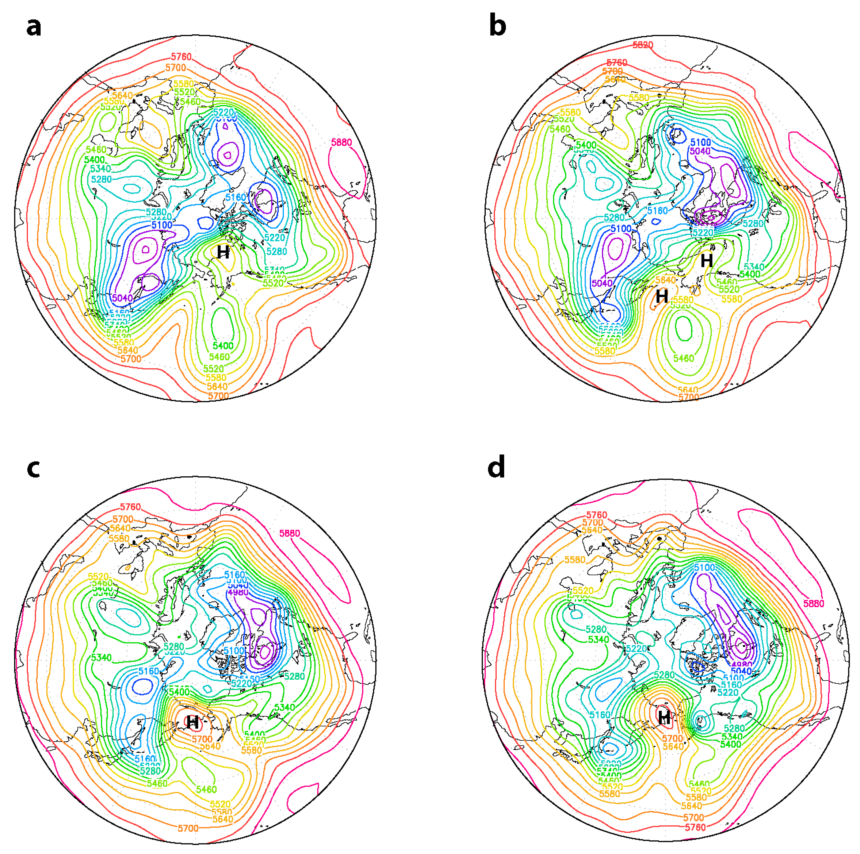
Figure 2.
As in Figure 1, except for (a) the onset time (1200 UTC 24 February 2017) and (b) peak intensity (1200 UTC 4 March 2017).
Figure 2.
As in Figure 1, except for (a) the onset time (1200 UTC 24 February 2017) and (b) peak intensity (1200 UTC 4 March 2017).
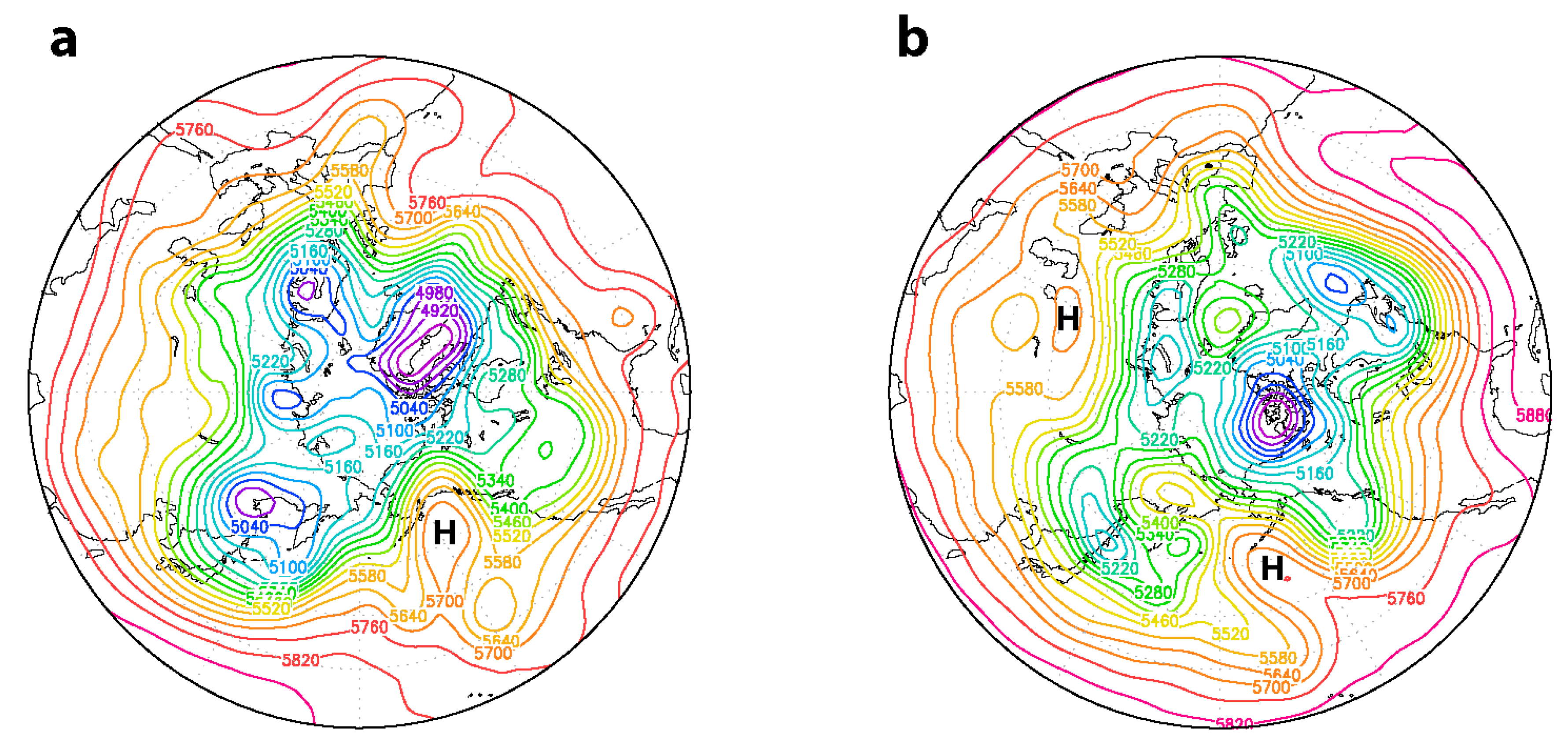
Figure 3.
Adapted from [13], (a,c) the block intensity (BI) as defined by [24] (ordinate) for the event studied in winter 2014 versus date in January and February 2014 and February and March 2017, respectively, (abscissa) (left), (b,d) the (Integrated Regional Enstrophy (IRE) (s−2) (ordinate) and days following the onset period in January and February 2014 and February and March 2017, respectively, (abscissa) (right).

Table 1.
Values for Block Intensity (BI), IRE, and Kolmogorov Smirnov Entropy ( KSE) during the lifecycle of the winter 2014 blocking event studied here, and the onset period as well as the mid-life intensification. The units for IRE are shown and BI and KSE are without units.
Table 1.
Values for Block Intensity (BI), IRE, and Kolmogorov Smirnov Entropy ( KSE) during the lifecycle of the winter 2014 blocking event studied here, and the onset period as well as the mid-life intensification. The units for IRE are shown and BI and KSE are without units.
| Block Period | BI | IRE (×10−6 s−2) | KSE |
|---|---|---|---|
| Onset Intensification 1 | 6.90 | 2.56 | 0.86 |
| Mid-block Intensification | 6.46 | 2.57 | 1.39 |
| Block Lifetime | 5.93 | 2.49 | 0.75 |
1 Due to the algorithm used to calculate KSE, the value obtained was the mean from 14 to 24 January 2014, while for the IRE the range of dates was 20–24 January 2014, and BI could only be 23–24 January 2014, since a block must be present for BI to be calculated.
Table 2.
As for Table 1, except for the winter 2017 blocking event studied here.
Table 2.
As for Table 1, except for the winter 2017 blocking event studied here.
| Block Period | BI | IRE (×10−6 s−2) | KSE |
|---|---|---|---|
| Onset Intensification 2 | 5.30 | 4.06 | 1.79 |
| Mid-block Intensification | 4.57 | 3.53 | 1.38 |
| Block Lifetime | 4.42 | 3.46 | 1.09 |
2 KSE was obtained from 15 to 25 February 2017, while for the IRE was 20–24 February 2017, and BI could only be 23–24 February 2017, since a block must be present for BI to be calculated.
© 2017 by the authors. Licensee MDPI, Basel, Switzerland. This article is an open access article distributed under the terms and conditions of the Creative Commons Attribution (CC BY) license (http://creativecommons.org/licenses/by/4.0/).
Share and Cite
MDPI and ACS Style
Jensen, A.D.; Lupo, A.R.; Mokhov, I.I.; Akperov, M.G.; Reynolds, D.D. Integrated Regional Enstrophy and Block Intensity as a Measure of Kolmogorov Entropy. Atmosphere 2017, 8, 237. https://doi.org/10.3390/atmos8120237
AMA Style
Jensen AD, Lupo AR, Mokhov II, Akperov MG, Reynolds DD. Integrated Regional Enstrophy and Block Intensity as a Measure of Kolmogorov Entropy. Atmosphere. 2017; 8(12):237. https://doi.org/10.3390/atmos8120237
Chicago/Turabian StyleJensen, Andrew D., Anthony R. Lupo, Igor I. Mokhov, Mirseid G. Akperov, and DeVondria D. Reynolds. 2017. "Integrated Regional Enstrophy and Block Intensity as a Measure of Kolmogorov Entropy" Atmosphere 8, no. 12: 237. https://doi.org/10.3390/atmos8120237
Note that from the first issue of 2016, this journal uses article numbers instead of page numbers. See further details here.