Energy Distribution of X-rays Produced by Meter-Long Negative Discharges in Air


1
Ångstrom Laboratory, Division of Electricity, Department of Engineering Sciences, Uppsala University, Box 534, SE-75121 Uppsala, Sweden
2
Institute for the Study of Earth, Oceans, and Space, University of New Hampshire, Morse Hall 309, 8 College Road, Durham, NH 03824, USA
*
Authors to whom correspondence should be addressed.
Atmosphere 2017, 8(12), 244; https://doi.org/10.3390/atmos8120244
Submission received: 11 September 2017
/
Revised: 29 November 2017
/
Accepted: 30 November 2017
/
Published: 6 December 2017
Abstract
:The energy deposited from X-rays generated by 1 m long laboratory sparks in air created by 950 kV negative lightning impulses on scintillated detectors was measured. Assuming the X-ray energy detected in such sparks results from the accumulation of multiple photons at the detector having a certain energy distribution, an experiment was designed in such a way to characterize their distribution parameters. The detector was screened by a copper shield, and eight series of fifteen impulses were applied by stepwise increasing the copper shield thickness. The average deposited energy was calculated in each series and compared with the results from a model consisting of the attenuation of photons along their path and probable photon distributions. The results show that the energy distribution of X-ray bursts can be approximated by a bremsstrahlung spectrum of photons, having a maximum energy of 200 keV to 250 keV and a mean photon energy around 52 keV to 55 keV.
1. Introduction
It is now a well observed fact that electrical discharges produce high energetic radiation from very soft X-rays in few kilo electron volts up to X-rays and gamma rays having several mega electron volts (Moore et al. [1]; Dwyer et al. [2,3]; Rahman et al. [4]; Nguyen et al. [5]; March and Montanyà, [6]; Kochkin et al. [7]). Experiments show that not only lightning flashes but also laboratory discharges generate X-rays (as first shown by Dwyer et al. [3]). The exact mechanism that leads to the generation of X-rays in laboratory sparks is still under investigation. It has been suggested, however, that the field enhancements caused during streamer encounters could be one possible mechanism that generates X-rays (Cooray et al. [8]). During these encounters, electrons could be accelerated beyond the threshold energies necessary for them to become runaways in the lower background fields. Even though the negative discharge development was simplified in the model, the main idea that the streamer encounters can cause X-ray emissions has been supported by recent experimental observations. In the case of positive breakdown in the laboratory, X-rays indeed appear when the positive streamers from the high voltage electrode meet the negative streamer that originates from the ground [7]. In recent studies, X-ray emissions were observed during the initiation of negative leaders from the high voltage electrode [9]. Even in this case, encounters occur between positive streamers originating from the space stem and the negative streamers originating from the high voltage electrodes. However, a recent simulations on runaway electron generation and X-ray emission questioned this mechanism [10,11,12]. However, as discussed in Section 5.4 of [9], the action of the electric field on the acceleration of electrons is underestimated in [10].
Energy distribution of X-ray photons generated by laboratory discharges is of interest in understanding the mechanism of X-ray generation. This is the case because it provides information concerning the maximum and average energies to which the electrons are accelerated. This information in turn can be used to test the predictions of the suggested mechanisms. However, in practice, measuring the energy of individual photons is difficult due to various reasons. Due to various constraints in methods used to detect these X-rays, it is difficult to quantify the measured X-ray radiation in both time domain and energy domain. This difficulty arises mainly because of limitations in detectors. Detection of X-ray bursts from electrical discharges is typically measured using scintillation detectors.
When an X-ray burst, generated from an electrical discharge, hits a scintillator crystal in an X-ray detector, each X-ray photon produces several visible light photons. These photons are collected by the cathode of the photo multiplier tube (PMT) attached to the scintillator and are converted to an electrical current which is multiplied by each stage in the PMT and is finally fed to a transient recorder. This mechanism is perfectly capable of resolving an X-ray spectrum correctly if certain conditions are satisfied. But these scintillated detectors produce higher output compared to individual photon energy when several X-rays photons in the burst hit the detector during the combined rise time of the measurement system and detector (depending on the surface area of the scintillator crystal, the distance from the source and the fluence of the photons, this could be a few photons to tens of photons). On the other hand, if the depth of the scintillator crystal is not thick enough to completely stop an X-ray photon, it might not produce an output at all or produce a smaller output. In cases, where a low energetic photon(s) immediately follows a very high energetic photon(s) within the decay time of the detector (250 ns in a typical NaI(Tl) detector), low energetic photon(s) may not be successfully detected.
In order to quantify X-ray energies from electrical discharges, the scintillation detectors could be shielded using attenuating material like lead. This is especially helpful where the X-ray detector produces an output higher than that of individual photon energy due to the accumulation of multiple photons. Previously, experiments were carried out with lead-shielded detectors along with unshielded detectors in measuring X-rays produced by rocket triggered lightning (Dwyer et al. [2]) and also laboratory discharges (Dwyer et al. [3]). These experiments also indicate that the measured energy from the unshielded detectors is higher than the individual X-ray photon energy of the associated bursts where the total deposited energy of an individual burst could be several MeV. In another study, Dwyer et al. [13] reported that the average photon energy could be around 230 keV while the total deposited energy could be as high as 50 MeV. Work carried out by Kochkin et al. in [7,14] using attenuators also reported X-ray photon energies on the order of 200 keV. In a detailed study, by assuming certain distributions for X-ray fluence and for photon energy, Carlson et al. [15] reported that the experimental results of X-rays from 1 MV electrical discharges can be modelled by an exponential X-ray distribution having a mean around 86 keV. Kochkin et al. [16] predicted that the mean energy of such sparks, when an exponential distribution is assumed, is 160 keV using a Monte Carlo model for electron and photon dynamics in an experimental setup with lead attenuators.
This paper describes an experiment carried out using attenuators and a model for the X-ray energy distribution to match the experimental results.
2. Experiment
The experimental study reported here was conducted at the high voltage laboratory of Uppsala University, Sweden. Figure 1 shows the approximate arrangement of the experiment schematically. A rod-sphere air gap was used at atmospheric pressure where the rod was made of brass and had a diameter of 10 mm. A sphere of diameter 2.1 cm was used as the anode. A negative so-called standard lightning impulse voltage (the impulse front time is 1.2 μs and the time to half value is 50 μs) was applied to the rod, defining the rod as the cathode. The gap length was 95 cm. The voltage impulse was generated by using a Marx impulse voltage generator (SGSA 1000-50, Haefely Test AG, Basel, Switzerland). In this experiment the charging voltage was 950 kV.
The voltage across the gap, the current through the gap and the emission of X-rays produced by the laboratory spark were measured. A capacitive impulse voltage divider (CS 1000-670, Haefely Test AG, Basel, Switzerland) was used to measure the voltage. The current was measured using a current transformer (Pearson model 411) at the grounded end. Both the voltage and the current were measured by a data acquisition card (Dias 733, Haefely Test AG, Basel, Switzerland) connected to a PC. The X-rays were measured using a NaI(Tl) scintillator of size 76 mm × 76 mm assembled with a photomultiplier tube (PMT) (model 3M3/3, Saint-Gobian Crystals, Hiram, OH, USA). The direct anode output of the NaI(Tl)/PMT was then connected to a fibre-optic transmitter (LTX-5515, Terahertz Technologies Inc., Oriskany, NY, USA). The whole detector system, consisting of scintillator, PMT and PMT base and the LTX-5515 fibre optic transmitter together with 12 V battery that supplied power to the detector system, was placed inside a 0.31 cm thick aluminium box. The box was then placed 105 cm away from the anode electrode on the grounded metal floor of the high voltage hall. The measured X-ray signal was then sent to a transient recorder (SL1000, Yokogawa Test & Measurement Corporation, Tokyo, Japan) via the fibre optic transceiver. The time synchronization of voltage, current and X-ray signal was achieved by splitting the current signal and also feeding it to the Yokogawa SL1000 recorder. The X-ray detector was calibrated using a 137Cs source.
The experimental setup used in this work is very similar to the experimental setup described in our previous work [17], with the primary difference being the use of attenuators surrounding the X-ray detector assembly as described next.
First a series of 15 sparks was applied where the NaI(Tl) detector was used un-shielded. Then a further 120 sparks were applied in 8 series with 15 sparks per series by covering the NaI(Tl) detector with copper shields of increasing thickness. This was achieved by using a copper sheet of thickness 0.3 mm to construct a shield which covers the scintillator crystal of the detector completely. This effective shield thickness varied from 0.3 mm to 2.4 mm by using a single layer up to 8 layers of copper shields in each series.
3. Results
The resulting waveforms of voltage, current and X-ray are very similar to what has been described in our previous work in [17]. A typical waveform from this experiment with X-ray signal, the applied voltage and the breakdown current at the ground is very much similar to the waveform shown in Figure 2 of [17]. The X-rays were mostly detected just before breakdown and about 250 ns prior to the current peak. The timing of the X-ray peak is discussed in detail in our previous work in [17]. In three sparks out of the total 135 sparks, an X-ray peak, occurring earlier in time, coinciding with the crest of the voltage, was also observed. The energy from these X-ray peaks was ignored when the average is calculated because these peaks were clearly separated from the typical X-ray peaks making them difficult to fit in the simulation model which is discussed in Section 4. The measurement system was not saturated in any of the 135 sparks.
Statistics of the X-ray detector output for the total 9 series of 135 sparks are tabulated in Table 1 showing the average, maximum and standard deviation of total detected energy in each series of 15 sparks. Additionally, the number of zero energy detections out of the total 15 sparks in each series is given.
When calculating the average of the total detected energy, cases where no X-rays were detected were included in the sample as a zero energy detection. This is justified by the following facts. A detection rate close to 100% was observed for the series where no copper shield is used. In addition, during the previous experiment described in [17] with the same experimental configuration, a detection rate close to 100% was observed. Hence, the zero energy detections in subsequent series, where copper shields exist, could be attributed to the absorption of photons by copper shields. Therefore, when taking the average, zero total energy cases should be considered to compare with results from the numerical model which will be described in Section 4.
The average of the total energy detected in each series is plotted against copper thickness in Figure 2. In spite of the two anomalies for copper shield thickness of 0.3 mm and shield thickness of 2.1 mm, the average energy data in above Table 1 could be fitted to a curve of first order exponential form with a tendency to show higher copper shield thickness reducing the average of the total detected energy.
As can be seen from Figure 2, each series has a standard deviation which is rather high. From our previous experience with X-ray measurements from very similar experiments of ~1 MV sparks, we observed that a higher number of sparks would not necessarily reduce the standard deviation of these measurements. This higher standard deviation could primarily be attributed to the initial distribution of the number of X-ray photons, variations of their energy spectrum in each spark, non-isotropic directional emission of photons from the spark and the varying efficiency of the detector system to a lesser extent.
4. Numerical Modelling, Comparison with Experimental Results and Discussion
4.1. Numerical Model
As evidenced by the experimental results, the X-ray fluence, measured at a given location, has a certain distribution caused by both varying luminosity of the photon bursts at the source and also by the possible non-isotropic beaming of photons. The energy spectrum of each spark itself could also vary, and the spectrum parameters are distributed in reality. In this study, because the distribution of photon energy is the primary concern, we have chosen to model only the energy spectrum of photons with unknown distribution parameters. The exclusion of distributions of fluence and detector efficiency from the numerical model makes it possible to conduct a more meaningful comparison of modelled results and experimental data, with fewer unknown parameters. This exclusion is further justified by the fact that, taking the average of the total detected energy of a series of sparks experimentally, the effect of those unknown distributions is implicitly included in the modelled result.
The experimental data provide the net total energy of the X-ray photons, after they penetrate copper shield of varying thickness and finally accumulate in the detector. In order to extract the photon energies from these data, it is necessary to determine the spectrum of X-ray photon energies that will satisfy the experimental data.
In almost all sparks where X-rays were detected, only a single X-ray burst was detected. Therefore, it is reasonable to assume that the energy detected by the detector is the accumulated energy of multiple photons absorbed by the detector within the rise-time of the detection system. If the spectrum and the number of photons are known at the origin of X-rays, then the total energy detected by the NaI(Tl) detector could be calculated for each data point in Figure 2 by calculating the attenuation of X-ray photons along their path from the source to the detector and integrating the resultant photon intensity curve with respect to energy.
Let us consider the spark to be an isotropic point source of X-ray photons and the total number of photons at the source for a given energy bin to be denoted by (the differential photon energy intensity). Then, let the function be the effective number of photons within the same energy bin at the source confined to a solid angle Ω (calculated using the distance from the detector to the source, and the surface area of the detector, ). Thus, can be calculated by multiplying by the factor as given in Equation (2). The function defines both the spectrum and the fluence of X-rays in this case.
Thus, the total number of photons confined to the solid angle Ω having an energy from to at the source is given by the integration with respect to energy,
and the total energy of the photons at the source confined to the solid angle Ω is given by the integration,
Now, in order to calculate the total detected energy by the NaI(Tl) X-ray detector, the attenuation of X-ray photons defined by function along their path from the origin to the detector surface should be considered. The attenuation from air (roughly 139 cm distance between the middle of the spark gap and aluminium box), aluminium enclosure, which is 3.1 mm thick, and the copper shield of varying thickness are considered in this case.
For a given intensity , the attenuation of mono energetic photons due to a mass of a certain material with thickness , density and attenuation coefficient is given by,
where is the intensity after the attenuation, and the term , which is dependent of the energy, is called the mass attenuation coefficient of the material considered for a given energy E.
Combining Equations (4) and (5), we can derive the total detected energy by the detector assuming a 100% absorption efficiency,
which is equal to the integration of the attenuated spectrum multiplied by energy, with respect to energy. Additionally the integration of the attenuated result shown in Equation (7) gives the total number of photons detected by the detector.
The NaI(Tl) X-ray detector used in this experiment was equipped with a 3″ × 3″ (i.e., 76 mm diameter, 76 mm thick) solid scintillator crystal. According to the manufacturer, a scintillator having NaI(Tl) crystal of thickness 76 mm has a roughly 80% absorption efficiency for 1 MeV photons and almost 100% absorption efficiency for 500 keV photons. Since we do not expect MeV range photons from a discharge of applied voltage of 950 kV, it is a fair assumption that the detector has almost 100% absorption efficiency for the X-ray photons considered in this experiment. This makes it possible to directly compare the results from Equations (6) and (7) with experimental results.
The mass attenuation coefficients, , for air, copper and aluminium for varying X-ray energies could be obtained from the NIST X-ray mass attenuation coefficient database (NISTIR 5632). Because is energy dependant and given in tabular format, the integrations in Equations (6) and (7) could only be solved numerically (even when an analytical expression for is known).
As can be seen from Equation (7), depending on the solid angle Ω and the initial fluence of photons generated at the source within the energy range to , could also be zero (because in order to get the number of photons from the integration, the result should be rounded off to a whole number). This is also evident experimentally with sparks where no X-rays are detected.
Because the function governing the spectrum and number of photons at the source, , is unknown, possible analytical expressions for X-ray spectrum for a laboratory spark should be considered. It is also evident that for a given analytical probability density function (or a differential intensity function) governing the photon spectrum, the function (which defines the total number of photons emitted at the source for a given energy) is simply the multiplication by a constant of proportionality .
In order to find an expression for the distribution of X-ray energy, one has to first find the distribution of electron energies involved in the bremsstrahlung process. Additionally, the bremsstrahlung differential cross-section relevant to the X-ray generation in electrical discharges in air for different ranges of electron energies should also be calculated. Using a combination of theoretical models for the generation of run-away electrons, Monte Carlo simulations of the electron energy and path, and considering the so-called Bethe-Heitler cross section for electron-nuclei bremsstrahlung, the photon fluence has been modelled previously in [16]. But photon energy spectrum is still arbitrarily assumed to be exponential in this study.
A similar approach is used in this study. A probable energy spectrum for photons is assumed first. Then, using attenuation of the photons, energy deposited at the X-ray detectors is calculated numerically. This result is then compared with experimental data. Two such possible spectrums for photons are considered in this study. The first is a bremsstrahlung spectrum, in its simplest and most crude form of Kramers’ law with an unknown maximum energy, assuming X-rays are primarily produced by the bremsstrahlung process between electrons and nitrogen atoms. The second is an exponential photon distribution with an unknown mean energy.
For both cases, the unknown parameters, the number of photons at the source and at the detector, the total energy produced at the source and the total energy absorbed by the detector could be calculated by defining the arbitrary function with analytical expressions from selected spectrums. In addition to these probable photon distributions, an extreme case where a burst of mono energetic photons is also considered for comparison purposes.
4.2. Simulation and Results with Kramers’ Law
The selection of Kramer’s law as the rule governing the X-ray spectrum is justified not because of any theoretical or experimental evidence of its validity but simply because it provides a rough approximation of a X-ray photon distribution for a bremsstrahlung process of a nearly mono-energetic electron beam hitting a target. In other words, it is reasonable to take this crude approach because the distribution of electrons themselves is not yet known. On the other hand, as can be seen later from Equation (11), the distribution of X-ray energies with this approach tends to follow a distribution of the order which is not significantly different from the assumptions made in previous studies. One can argue that, since electrons themselves have an energy distribution, the superposition of Kramers’ distributions for different electron energies would produce a more accurate photon distribution. But this approach is not considered because as mentioned earlier, Kramers’ rule is used somewhat arbitrarily in this case and superposition is deemed unnecessary.
In this case, we also assume the bremsstrahlung process happens in the spark gap itself but not at the electrodes. Thus, we consider the bremsstrahlung process between electron and nitrogen atoms primarily. The differential intensity I of the bremsstrahlung X-rays photons at any given energy in the spectrum is given by Kramer’s Law as
where Z is the mean atomic number (in this case for nitrogen), K is a constant of proportionality, E is the energy of generated photons and is the energy of the mono energetic electron beam and also the maximum energy of X-ray photons. The intensity is zero when (the Duane-Hunt limit) but approaches infinity () as approaches zero.
Now, for the case of Kramers’ law, , can be written using Equations (2), (8) and (9) as
By merging all constants together, above expression can be re written as
where the parameter is the product of the geometric distribution factor and other two constants and . By substituting for in (6), a simulated best fit curve of detected energy vs the coper thickness similar to the experimental results as shown in Figure 2 can be generated for two unknown parameters and . By comparing this curve with the experimental curve shown in Figure 2, the best possible combination of and is obtained.
During this process all the numerical integrations are calculated using trapezoidal rule with an energy step size of 0.1 keV. The minimum energy necessary to calculate the integration in (6) is considered to be 5 keV, which is derived from the maximum sensitivity of the detector system. But in reality, any value of minimum energy up to about 15 keV would give the same results, because air and aluminium box along the photon path produce a lower cut-off energy around 15 keV. The mass attenuation coefficients , for each energy step are calculated by interpolating the tables obtained from NISTIR 5632 database for different materials.
It is interesting to observe the attenuation of the photons along their path from the source to the detector, since the parameters and are now known. This gives a picture of how the number of photons confined to Ω decreases along their path from source to the detector. The source photon intensity confined to Ω, , is shown in Figure 3. It is also evident from Equation (7) that the term, gives the attenuated intensity of photons due to different media along the path of photons. This attenuated intensity of photons along their path is shown in Figure 4 and Figure 5 considering the attenuation of air, aluminium and copper. The total number of photons depicted in these figures is calculated by rounding off the integrated results to a whole number. The 15 keV lower cut-off energy due to attenuation is visible in Figure 4.
The final simulated results, assuming 100% efficient detection, and the experimental results are shown in Figure 6. We find a good agreement with the experimental data with and . However, before making any conclusions regarding the X-ray photon energies, it is necessary to determine the sensitivity of the results obtained for the changes to these two parameters. The result of a simple sensitivity analysis of the parameters relative to the simulated results is shown in Figure 7. Based on this analysis, it is concluded that the fits of the simulated and experimental results match only for the unique set of parameter values and .
The parameter , which is inherently an expression of number of photons, tends to influence the above plot in Figure 6 linearly, while the maximum energy has a greater influence on higher coper thickness of the plot. This is understandable because in order to penetrate thicker shields, photons with greater energies are required, and even a large number of low energetic photons cannot penetrate a thicker shield.
On the other hand, this result is also dependent on the shape of the generated spectrum. Even though there are modifications derived to the basic Kramers’ law for electron metal bremsstrahlung based on both experiments and theoretical models yielding accurate spectrums, such expressions for laboratory discharges where bremsstrahlung happens between electrons and air molecules and atoms (nitrogen and oxygen primarily) could not be found. If a bremsstrahlung spectrum, valid for X-ray production from discharges in air, is used instead of the basic Kramer’s law which is applied in the above simulation, the maximum energy would be different from the simulated value of 204 keV.
4.3. Simulation and Results with an Exponential Photon Energy Distribution
The choice of Kramers’ rule for photon distribution used above seems somewhat arbitrary and hence there could also be other distributions which also provide results in agreement with the experimental data. Therefore, an exponential energy distribution is also considered. Use of an exponential distribution is further relevant because previous statistical models used by Carlson et al. [15] and Kochkin et al. [16] have also assumed exponential photon energy distributions.
By using a similar approach as used in Equations (10) and (11), the differential intensity of X-rays photons at any given energy confined to a solid angle Ω, for an exponential distribution can be defined as
where is the mean energy of the photon distribution and is defined as the product of the geometric distribution factor and the coefficient of proportionality of the distribution.
By substituting for in (6) and utilizing the same approach as used previously for Kramers’ distribution, possible combinations of values for the unknown parameters and are obtained. In addition, these values are verified to be unique by utilising the same sensitivity analysis approach as described in Figure 7 for Kramers’ distribution.
The resultant photon intensities at the source , for varying copper thicknesses, and the final comparison of experimental and simulated results are shown in Figure 8, Figure 9 and Figure 10 respectively. The integration is carried out with a maximum energy of 950 keV (which is equal to the supply voltage across the gap, and hence the theoretical maximum energy of photons), a minimum energy of 5 keV and a step size of 0.1 keV.
4.4. Comparison of Distributions
Using Equations (3) and (4) it is possible to find the mean energy of the photons under Kramers’ rule and the exponential photon energy distribution. Additionally, Equations (1)–(3) could be used to calculate the total number photons generated at the source. The mean energies of detectable photons under Kramers’ distribution and exponential distribution, assuming a minimum threshold of 15 keV (derived from Figure 4 previously), are 52 keV and 54.5 keV respectively. The total number of detectable photons generated from the spark under Kramers’ and exponential distributions in sterad are 1.76 × 10⁵ and 1.7 × 10⁵ respectively (assuming that the X-rays are generated at the middle of the spark gap and the effective detector diameter is 76 mm). Additionally, as can be observed from Figure 8, the maximum energy under an exponential distribution is limited to about 250 keV which is not much higher than 204 keV, the maximum found under Kramers’ distribution. From these results it can be concluded that both the distributions yield comparable results.
As an extreme scenario of a chosen spectrum, a case, where X-rays generated from the spark are mono-energetic, could be considered. Assuming a mono energetic X-ray beam of 17 photons confined in the solid angle Ω with an energy of 83 keV, we get a close match to the experimental results as shown below in Figure 11. But, in reality, X-ray photons have different energies and the close match between the simulated and experimental data could be due to several reasons. First, it is possible that the range of the variation of the energy of individual photons is not very large, and for this reason, mono energetic spectrum could provide a close match within experimental uncertainties. The second possibility is that the average energy of the photons selected here provides a close match to the average energy of the photons generated in the experiment. The important point is that the average energy of the photons that is necessary to provide a close fit is not far from the values predicted from other theoretical considerations (Carlson et al. [15] and Kochkin et al. [16]).
5. Conclusions
The experimental data presented in this paper, in combination with numerical modelling, show that the maximum energy of the X-ray photons generated in 1 m long negative sparks is in the order of 200 keV to 250 keV with a mean energy around 50 keV to 55 keV. The two types of distributions considered produce similar results for the mean energy and for the total number of photons. Despite being slightly different from previous estimates reported in [7,13,14,15,16], the values derived in this study are of the same order of magnitude as these previous estimates.
Acknowledgments
This work was supported by Swedish Research Council grant VR-2015-05026 and partly by the fund from the B. John F. and Svea Andersson donation at Uppsala University.
Author Contributions
Pasan Hettiarachchi prepared the experiment, constructed X-ray detectors and conducted the experiment, collected the data, analyzed the data and implemented the theoretical simulation in Matlab, and wrote the manuscript. Vernon Cooray generated the original idea, contributed to the writing of the manuscript and to both the simulation and analysis. Mahbubur Rahman also conducted the experiment together with Pasan Hettiarachchi and contributed to the simulation and analysis. Joseph Dwyer contributed by sharing his knowledge and expertise on X-ray measurements systems and contributed to the theoretical model and simulation.
Conflicts of Interest
The authors declare no conflict of interest.
References
- Moore, C.B.; Eack, K.B.; Aulich, G.D.; Rison, W. Energetic radiation associated with lightning stepped-leaders. Geophys. Res. Lett. 2001, 28, 2141–2144. [Google Scholar] [CrossRef]
- Dwyer, J.R.; Uman, M.A.; Rassoul, H.K.; Al-Dayeh, M.; Caraway, L.; Jerauld, J.; Rakov, V.A.; Jordan, D.M.; Rambo, K.J.; Corbin, V.; et al. Energetic radiation produced during rocket-triggered lightning. Science 2003, 299, 694–697. [Google Scholar] [CrossRef] [PubMed]
- Dwyer, J.R.; Rassoul, H.K.; Saleh, Z.; Uman, M.A.; Jerauld, J.; Plumer, J.A. X-ray bursts produced by laboratory sparks in air. Geophys. Res. Lett. 2005, 32. [Google Scholar] [CrossRef]
- Rahman, M.; Cooray, V.; Ahmad, N.A.; Nyberg, J.; Rakov, V.A.; Sharma, S. X rays from 80-cm long sparks in air. Geophys. Res. Lett. 2008, 35. [Google Scholar] [CrossRef]
- Nguyen, C.V.; van Deursen, A.P.J.; Ebert, U. Multiple X-ray bursts from long discharges in air. J. Phys. D Appl. Phys. 2008, 41, 234012. [Google Scholar] [CrossRef]
- March, V.; Montanyà, J. Influence of the voltage-time derivative in X-ray emission from laboratory sparks. Geophys. Res. Lett. 2010, 37. [Google Scholar] [CrossRef]
- Kochkin, P.O.; Nguyen, C.V.; van Deursen, A.P.J.; Ebert, U. Experimental study on hard X-rays emitted from metre-scale positive discharges in air. J. Phys. D Appl. Phys. 2012, 45, 425202. [Google Scholar] [CrossRef]
- Cooray, V.; Arevalo, L.; Rahman, M.; Dwyer, J.; Rassoul, H. On the possible origin of X-rays in long laboratory sparks. J. Atmos. Sol. Terres. Phys. 2009, 71, 1890–1898. [Google Scholar] [CrossRef]
- Kochkin, P.; Lehtinen, N.; van Deursen, A.L.P.; Østgaard, N. Pilot system development in metre-scale laboratory discharge. J. Phys. D Appl. Phys. 2016, 49, 42520. [Google Scholar] [CrossRef]
- Ihaddadene, M.A.; Celestin, S. Increase of the electric field in head-on collisions between negative and positive streamers. Geophys. Res. Lett. 2015, 42, 5644–5651. [Google Scholar] [CrossRef] [Green Version]
- Köhn, C.; Chanrion, O.; Neubert, T. Electron acceleration during streamer collisions in air. Geophys. Res. Lett. 2017, 44, 2604–2613. [Google Scholar] [CrossRef] [PubMed]
- Babich, L.; Bochkov, E. Numerical simulation of electric field enhancement at the contact of positive and negative streamers in relation to the problem of runaway electron generation in lightning and in long laboratory sparks. J. Phys. D Appl. Phys. 2017, 50, 455202. [Google Scholar] [CrossRef]
- Dwyer, J.R.; Saleh, Z.; Rassoul, H.K.; Concha, D.; Rahman, M.; Cooray, V.; Jerauld, J.; Uman, M.A.; Rakov, V.A. A study of X-ray emission from laboratory sparks in air at atmospheric pressure. J. Geophys. Res. 2008, 113. [Google Scholar] [CrossRef]
- Kochkin, P.O.; van Deursen, A.P.J.; Ebert, U. Experimental study on hard X-rays emitted from metre-scale negative discharges in air. J. Phys. D Appl. Phys. 2015, 48, 025205. [Google Scholar] [CrossRef]
- Carlson, B.E.; Østgaard, N.; Kochkin, P.; Grondahl, Ø.; Nisi, R.; Weber, K.; Scherrer, Z.; LeCaptain, K. Meter-scale spark X-ray spectrum statistics. J. Geophys. Res. Atmos. 2015, 120, 191–202. [Google Scholar] [CrossRef] [PubMed]
- Kochkin, P.O.; Köhn, C.; van Deursen, A.P.J.; Ebert, U. Analyzing X-ray emissions from meter-scale negative discharges in ambient air. Plasma Sour. Sci. Technol. 2016, 25, 044002. [Google Scholar] [CrossRef]
- Hettiarachchi, P.; Rahman, M.; Cooray, V.; Dwyer, J. X-rays from negative laboratory sparks in air: Influence of the anode geometry. J. Atmos. Sol. Terres. Phys. 2016, 154, 190–194. [Google Scholar] [CrossRef]
Figure 1.
The experimental setup consisting of the Marx generator, voltage divider, spark gap and the X-ray detector (seen from left to right, not in real proportions).
Figure 1.
The experimental setup consisting of the Marx generator, voltage divider, spark gap and the X-ray detector (seen from left to right, not in real proportions).
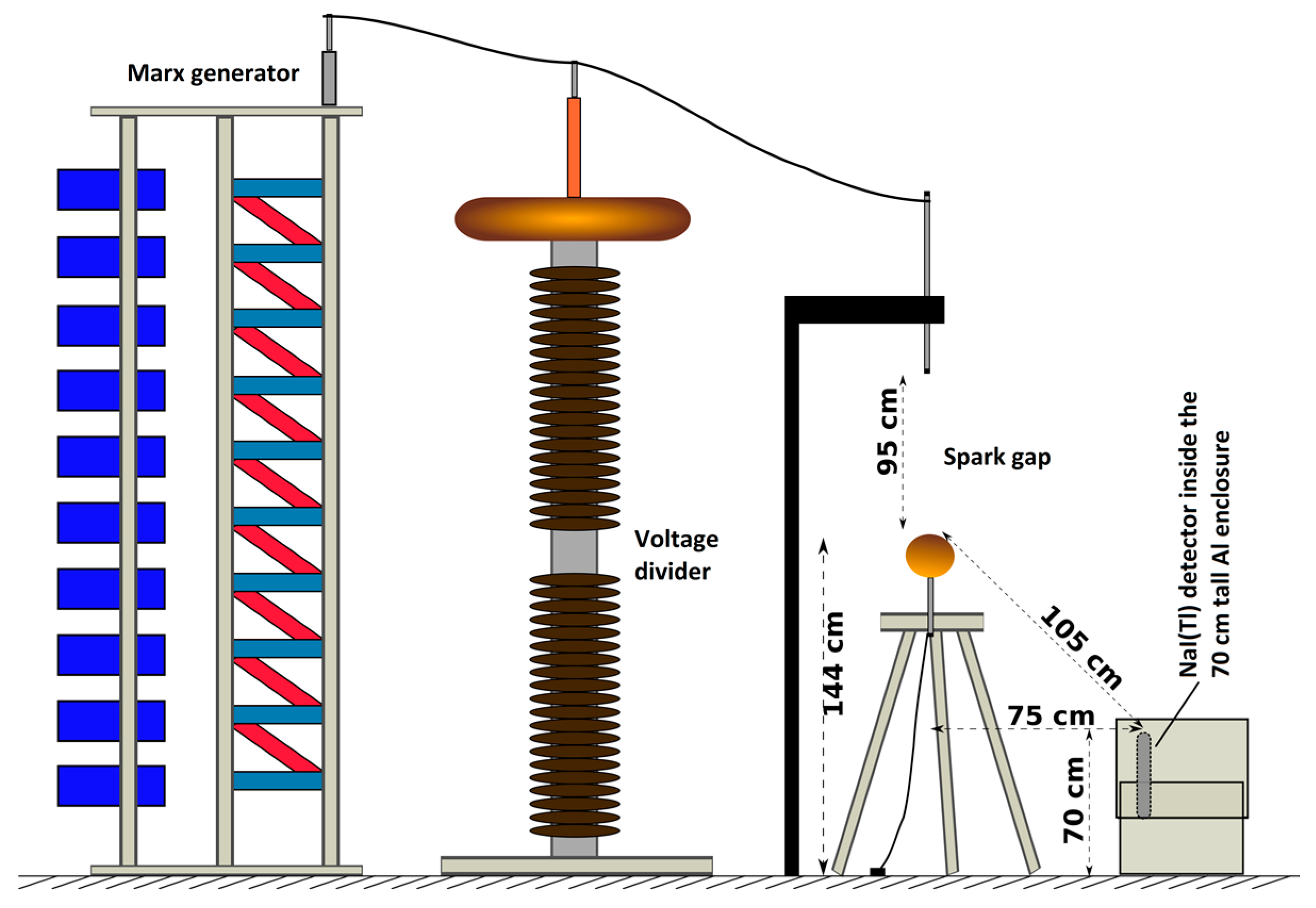
Figure 2.
Experimental results of the average total detected energy fitted to a curve with a first order exponential curve fit. The error bars indicate the standard deviation of each data point. The fit parameters are shown in the legend.
Figure 2.
Experimental results of the average total detected energy fitted to a curve with a first order exponential curve fit. The error bars indicate the standard deviation of each data point. The fit parameters are shown in the legend.
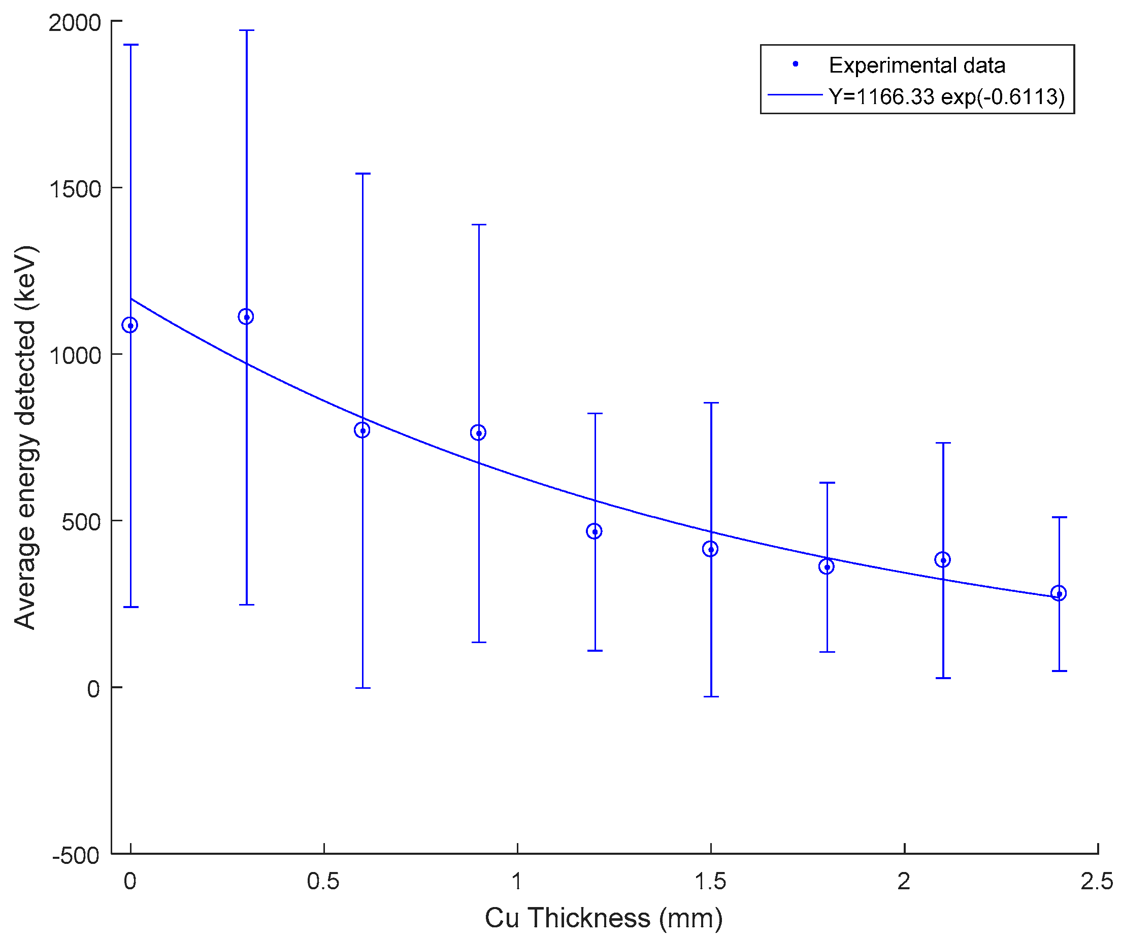
Figure 3.
A bremsstrahlung differential spectrum generated with Kramer’s law from an isotropic source confined to a solid angle Ω, , with maximum photon energy and the parameter . The choice of values for and is found by matching the final simulated results for Equation (6) with experimental results shown in Figure 2. The total number of photons, 57, and the total energy of photons at the source, 2024 keV, confined to the solid angle Ω, is obtained using Equations (3) and (4).

Figure 4.
Simulated X-ray intensity at the detector confined to a solid angle Ω after the attenuation of air and the aluminium box, . This is the case where no copper layers are used to cover the detector. Total integrated energy is 1253 keV and the total number of photons is 18 as shown in the legend.

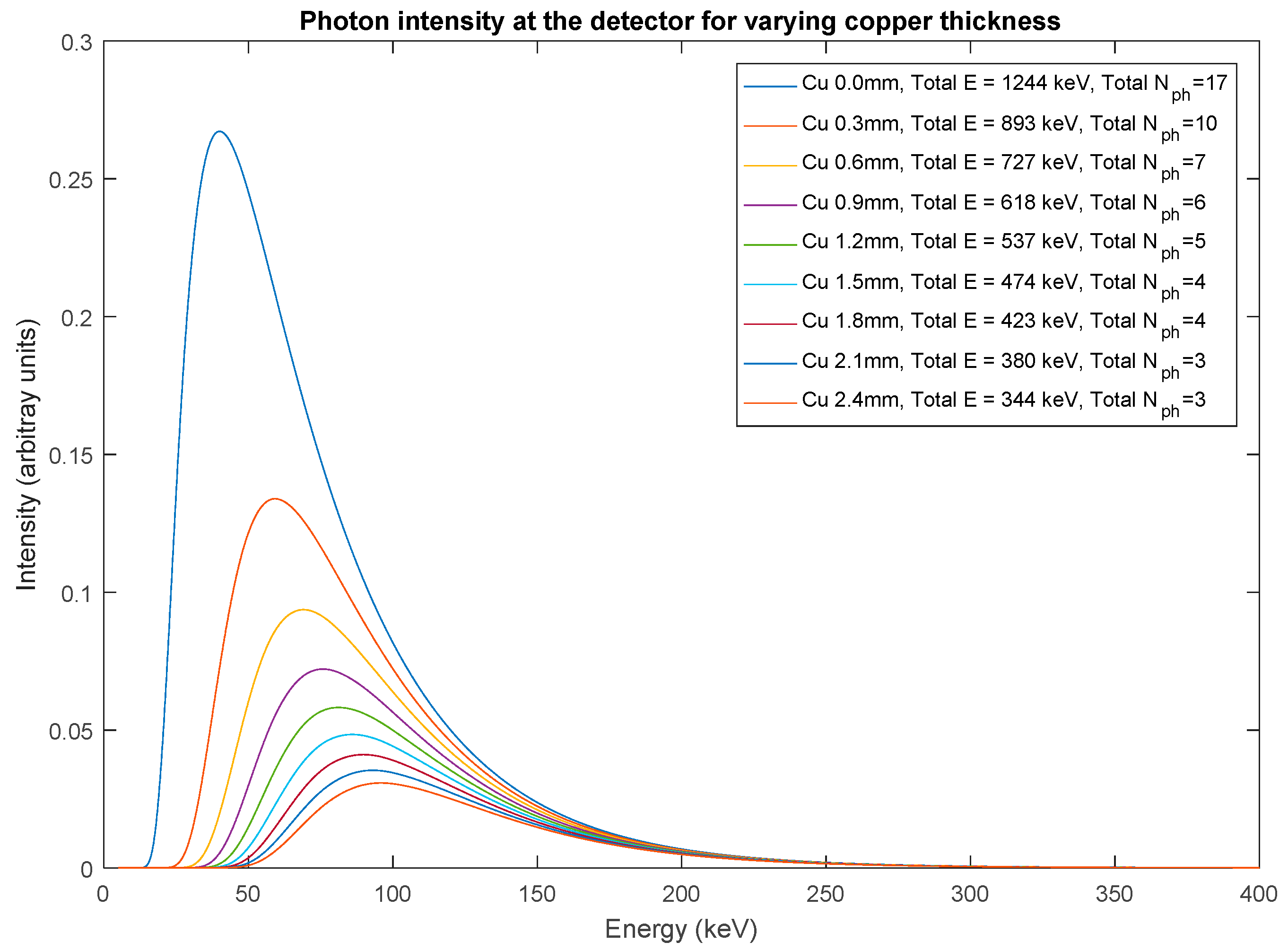
Figure 5.
Simulated X-ray photon intensities, confined to a solid angle Ω after the attenuation of air, aluminium box and copper shields with varying thicknesses. The total integrated energy and total number of photons are also given in the legend for different Cu shield thicknesses.
Figure 5.
Simulated X-ray photon intensities, confined to a solid angle Ω after the attenuation of air, aluminium box and copper shields with varying thicknesses. The total integrated energy and total number of photons are also given in the legend for different Cu shield thicknesses.

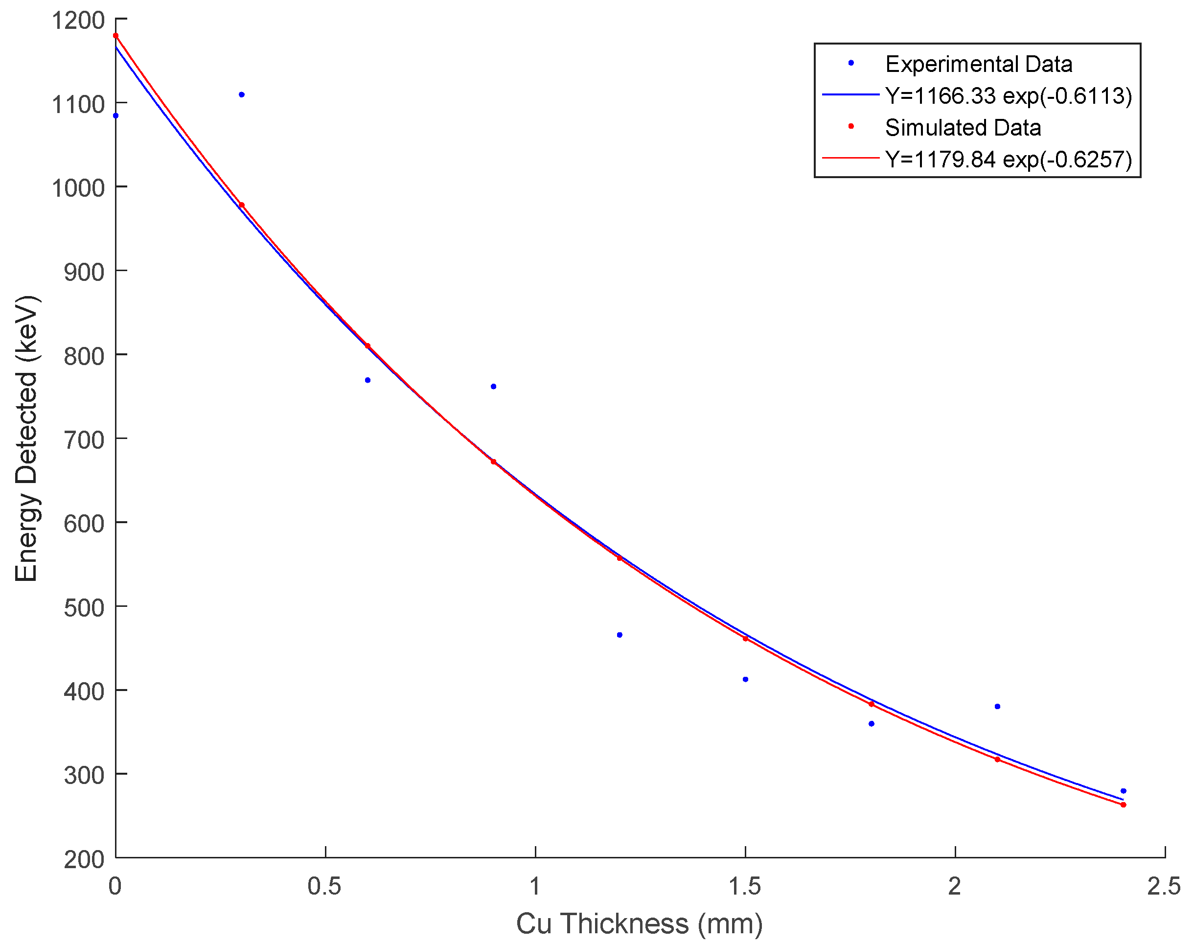
Figure 6.
Simulated vs experimental results for a photon distribution governed by Kramers’ law with and . The above values are chosen in such a way to obtain the best possible match between fitted curves of experimental and simulated results. Both curves for experimental and simulated results are fitted to a first order exponential curve with fit parameters shown in the legend.

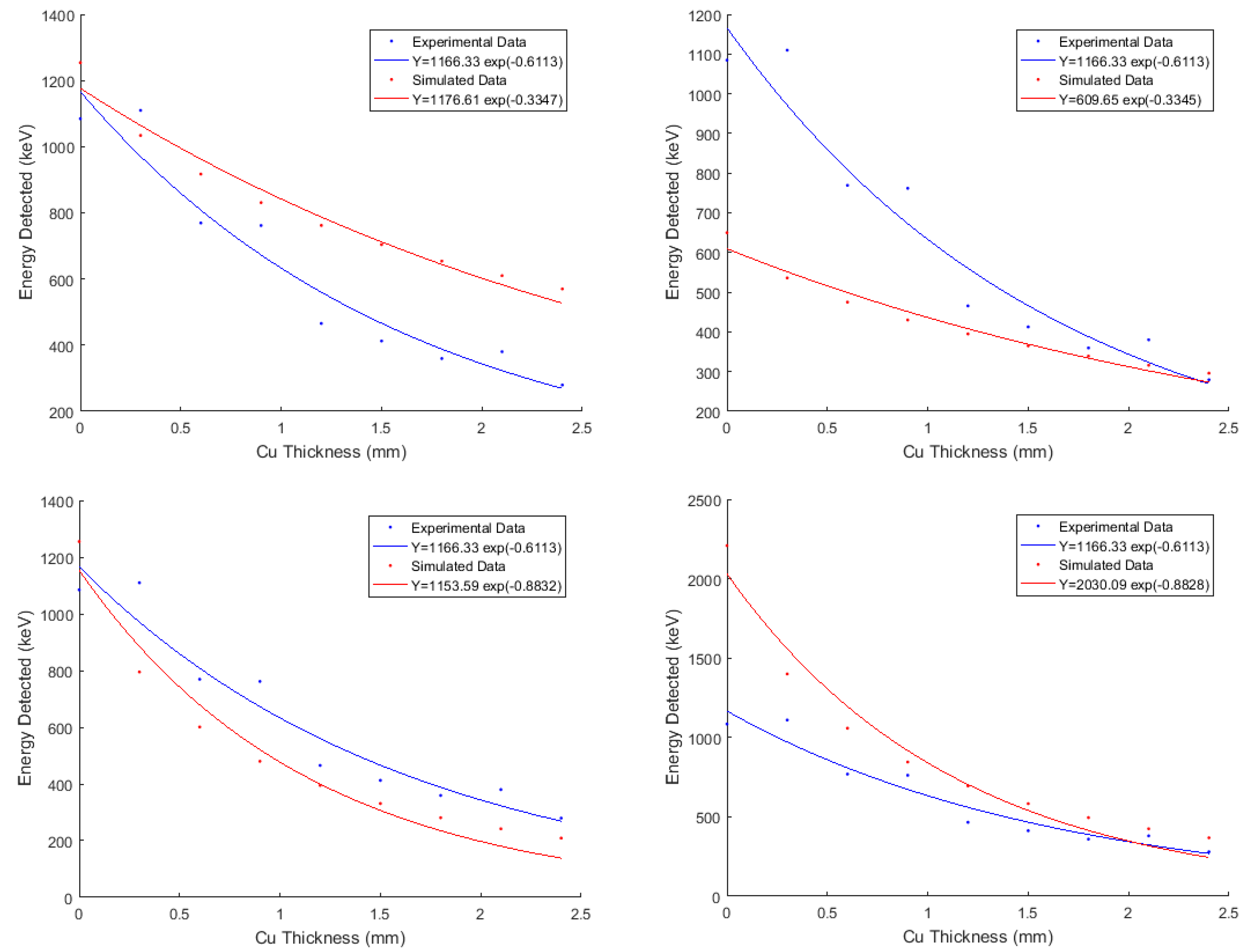
Figure 7.
Sensitivity of the simulated results to the parameters. The two upper plots are plotted with which is higher than the optimal, and in the upper left and in upper right plot. No value of could be found to match the experimental and simulated result. Similarly, with , which is lower than optimal is chosen in the bottom plots where in the bottom left and in bottom right plot. No value of could be found to match the experimental and simulated result.

Figure 8.
An exponential photon spectrum from an isotropic source confined to a solid angle Ω, , with characteristic mean photon energy and the parameter . The choice of values for and is found by matching the final simulated results for Equation (6) with experimental results shown in Figure 2. As can be seen from the curve, the effective maximum energy of photons is around 250 keV.
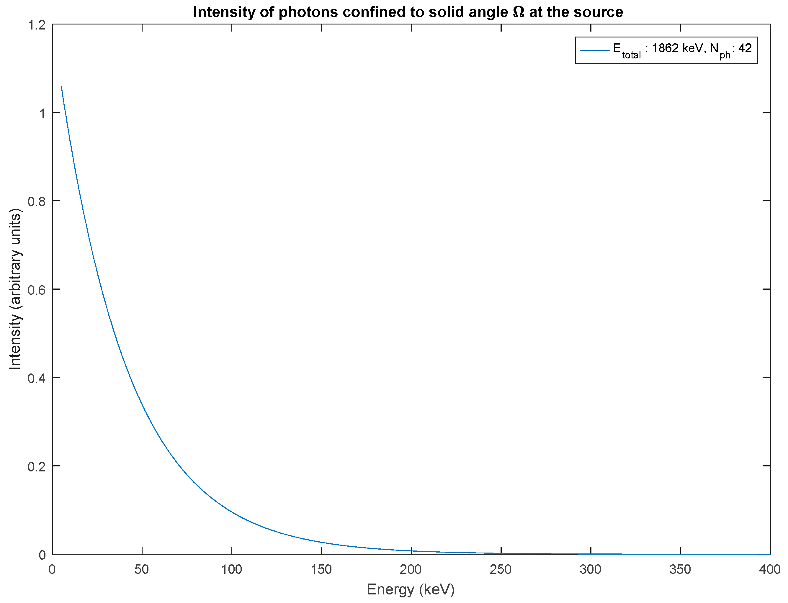
Figure 9.
Simulated X-ray photon intensities, confined to a solid angle Ω after the attenuation of air, aluminium box and copper shields with varying thicknesses or an exponential photon distribution with mean energy of the parameter . The total integrated energy and total number of photons are also given in the legend for different Cu shield thicknesses.

Figure 10.
Simulated vs. experimental results for an exponential photon distribution with and . The above values are chosen in such a way to obtain the best possible match between the experimental and simulated results. Both curves for experimental and simulated results are fitted to a first order exponential curve with fit parameters shown in the legend.
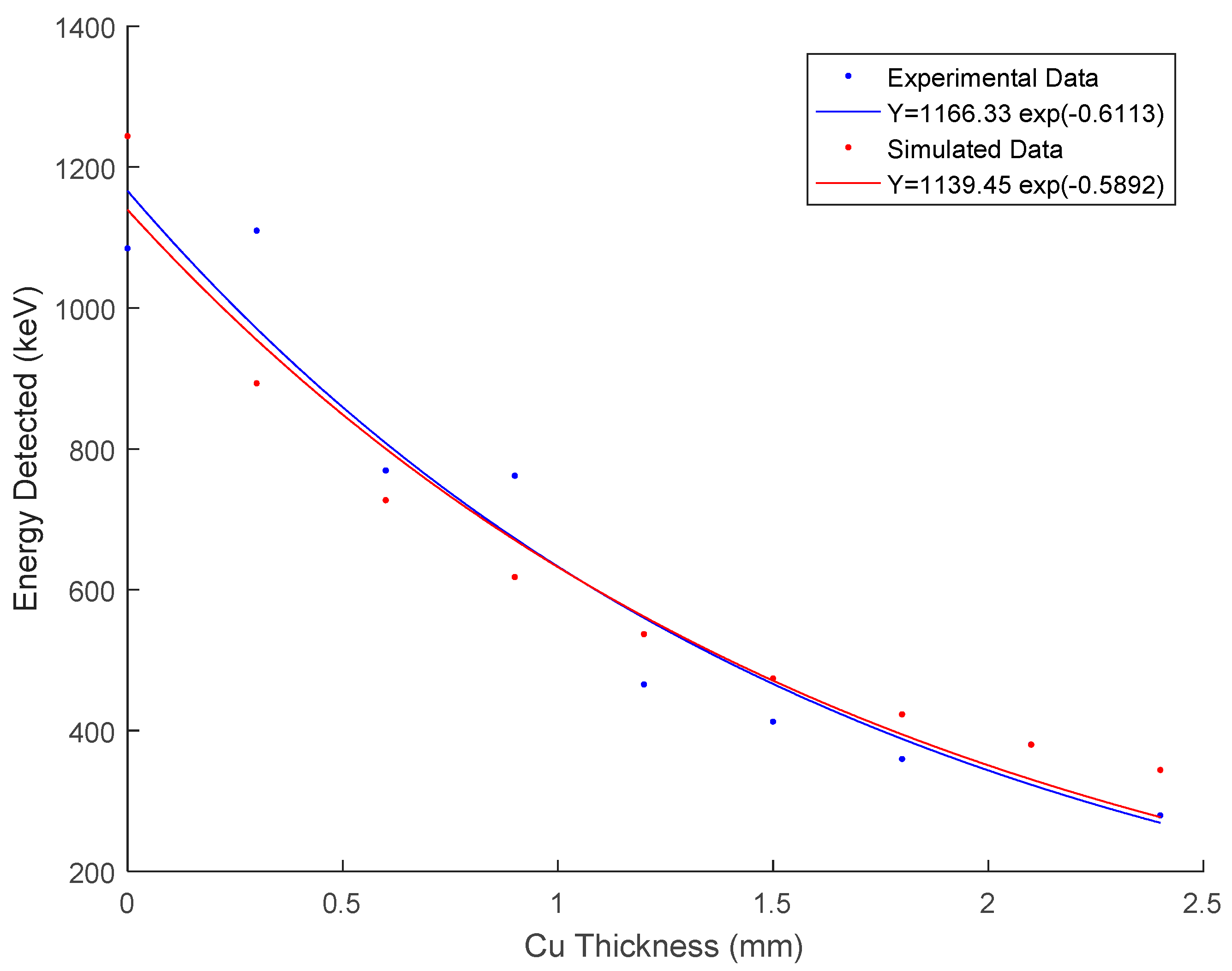
Figure 11.
Simulated vs. experimental results for a mono energetic X-ray burst of 17 photons with 83keV confined to solid angle Ω.
Figure 11.
Simulated vs. experimental results for a mono energetic X-ray burst of 17 photons with 83keV confined to solid angle Ω.


Table 1.
Average, minimum, maximum, standard deviation and zero detections of X-ray energy vs. Cu Shield thickness: The average is taken from each series consisting of 15 sparks with the given copper shield thickness surrounding the NaI(Tl) X-ray detector.
Table 1.
Average, minimum, maximum, standard deviation and zero detections of X-ray energy vs. Cu Shield thickness: The average is taken from each series consisting of 15 sparks with the given copper shield thickness surrounding the NaI(Tl) X-ray detector.
| Thickness of Cu Shield (mm) | 0.0 | 0.3 | 0.6 | 0.9 | 1.2 | 1.5 | 1.8 | 2.1 | 2.4 |
|---|---|---|---|---|---|---|---|---|---|
| Average X-ray Energy (keV) | 1085 | 1110 | 769 | 762 | 466 | 413 | 360 | 380 | 279 |
| Maximum Energy (KeV) | 3321 | 3662 | 2754 | 2294 | 1038 | 1238 | 1007 | 1354 | 734 |
| Standard Deviation (keV) | 844 | 862 | 772 | 627 | 356 | 441 | 254 | 353 | 231 |
| No. of Zero Detections Out of 15 | 1 | 1 | 2 | 1 | 4 | 6 | 2 | 3 | 4 |
© 2017 by the authors. Licensee MDPI, Basel, Switzerland. This article is an open access article distributed under the terms and conditions of the Creative Commons Attribution (CC BY) license (http://creativecommons.org/licenses/by/4.0/).
Share and Cite
MDPI and ACS Style
Hettiarachchi, P.; Cooray, V.; Rahman, M.; Dwyer, J. Energy Distribution of X-rays Produced by Meter-Long Negative Discharges in Air. Atmosphere 2017, 8, 244. https://doi.org/10.3390/atmos8120244
AMA Style
Hettiarachchi P, Cooray V, Rahman M, Dwyer J. Energy Distribution of X-rays Produced by Meter-Long Negative Discharges in Air. Atmosphere. 2017; 8(12):244. https://doi.org/10.3390/atmos8120244
Chicago/Turabian StyleHettiarachchi, Pasan, Vernon Cooray, Mahbubur Rahman, and Joseph Dwyer. 2017. "Energy Distribution of X-rays Produced by Meter-Long Negative Discharges in Air" Atmosphere 8, no. 12: 244. https://doi.org/10.3390/atmos8120244
Note that from the first issue of 2016, this journal uses article numbers instead of page numbers. See further details here.