Utilization of Global Precipitation Datasets in Data Limited Regions: A Case Study of Kilombero Valley, Tanzania


1
Department of Physical Geography, Stockholm University, 10691 Stockholm, Sweden
2
Department of Geography, Hydrology and Climate, University of Zurich, 8006 Zurich, Switzerland
3
The Nature Conservancy, Delmont, NJ 08314, USA
*
Author to whom correspondence should be addressed.
Atmosphere 2017, 8(12), 246; https://doi.org/10.3390/atmos8120246
Submission received: 3 October 2017
/
Revised: 16 November 2017
/
Accepted: 27 November 2017
/
Published: 7 December 2017
(This article belongs to the Special Issue Precipitation Variability and Change in Africa)
Abstract
:This study explored the potential for bias correction of global precipitation datasets (GPD) to support streamflow simulation for water resource management in data limited regions. Two catchments, 580 km2 and 2530 km2, in the Kilombero Valley of central Tanzania were considered as case studies to explore three GPD bias correction methods: quantile mapping (QM), daily percentages (DP) and a model based (ModB) bias correction. The GPDs considered included two satellite rainfall products, three reanalysis products and three interpolated observed data products. The rainfall-runoff model HBV was used to simulate streamflow in the two catchments using (1) observed rain gauge data; (2) the original GPDs and (3) the bias-corrected GPDs as input. Results showed that applying QM to bias correction based on limited observed data tends to aggravate streamflow simulations relative to not bias correcting GPDs. This is likely due to a potential lack of representativeness of a single rain gauge observation at the scale of a hydrological catchment for these catchments. The results also indicate that there may be potential benefits in combining streamflow and rain gauge data to bias correct GPDs during the model calibration process within a hydrological modeling framework.
Keywords:
bias correction; quantile mapping; satellite; reanalysis; interpolated; precipitation; HBV; Kilombero; Tanzania; Eastern Africa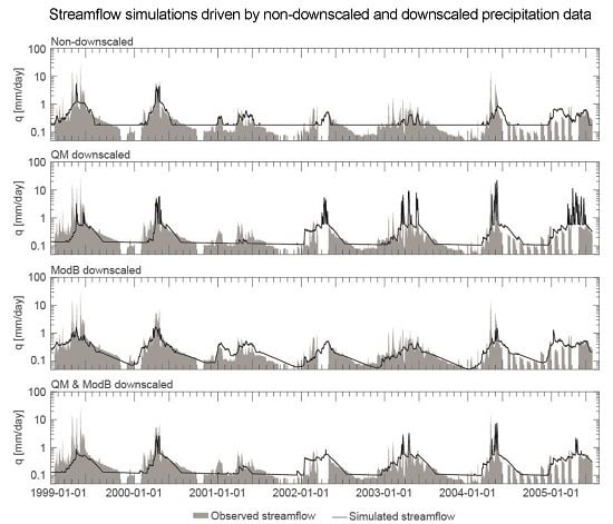
1. Introduction
Accessible and reliable precipitation observations are limited in large parts of the world. While central for hydroclimatological studies and development of water management schemes, precipitation observations are often based on discontinuous measurement records and have tendencies to contain discrepancies [1]. This deficiency in spatial and temporal coverage has motivated several attempts to create global precipitation datasets (GPDs) which could potentially be not only more temporally and spatially complete but also render more accurate precipitation estimates relative to the sparse data available via direct observations. If such improvements can be realized within GPDs, then these products would be very useful in data limited regions, especially those where the timing and amount of rainfall directly relate to economic and environmental sustainability [2,3].
For example, several studies have previously evaluated the quality of various GPDs in Eastern Africa both based on comparisons to precipitation estimates [4,5,6] and on their ability to produce accurate predictions from hydrological modelling [7,8,9]. With regards to the latter case, GPDs have been successfully implemented in hydrological modelling over a range of climatic zones, spatial scales and temporal resolutions [7,10,11,12]. While GPDs have shown promise to be a potential substitute for directly observed data in hydrological modelling applications, the performance of a specific GPD varies from region to region depending on, for example, complexity of terrain, availability of rain gauge data for bias correction and the temporal resolution considered [13,14,15,16,17]. Fundamentally, as all these factors can affect precipitation estimation accuracy and introduce non-linear error propagation into streamflow modelling [18,19]. Hence, there is need for investigations on the ability to utilize bias corrected GPDs in conjunction with hydrological models in data limited regions.
GPDs can be divided into three main categories: satellite-based products, reanalysis products and interpolated observed data products [20,21,22]. While each category can be considered to have various strengths and weaknesses in regional accuracy or applicability [23,24,25], all face performance issues related to the catchment size when being considered within a hydrological modeling framework [26]. Specifically, several authors have concluded that the ability of GPDs to estimate precipitation declines with decreasing target areas [23,27,28]. To tackle this issue, a number of bias correction techniques have been developed in order to potentially decrease GPDs precipitation estimate errors in smaller areas.
Bias correction techniques use empirical relationships between coarse resolution estimates and (for example) point observations to correct for systematic errors. Selecting a bias correction technique, thus, is inherently a function of data availability in a region. For example, Themeßl et al. [29] compared several bias correction (and empirical-downscaling) methods for regional climate model hindcast simulations in an area with a high rain gauge density. From that work, Quantile Mapping (QM) was shown to overall perform best and did particularly well for extreme events. Ringard et al. [30] further showed that QM could successfully reduce bias errors even in regions of sparse rain gauge network coverage by dividing the rain gauges into sub-groups representing different climate zones. However, the suitability of bias correction methods like QM in truly data-limited environments where GPDs are needed most in practice still needs to be explored.
Kilombero Valley (KV) (Figure 1), located in central Tanzania, is an example of such an environment (which is mirrored over much of Eastern Africa). KV’s general data limitations are troublesome as it has been targeted as a hot spot for agricultural development both in terms of increased annual crop production and cultivated area [31]. The goals of this development are increased food security and poverty alleviation [32]. As such, a call has been put forward for studies of all tributaries to the KV wetland and to the main river to improve understanding of current conditions and develop management strategies to avoid future deterioration of available water resources [33]. Given the limitations in observation data available for the region and emphasis on catchment-scale assessments [31], a first step could be to explore potentials and approaches for bias correction of GPDs to help fill gaps in time and spatial coverage of rainfall estimates and support modeling of streamflows [23].
In this study we investigate the possibility of using GPDs to simulate streamflow seasonality in the truly data limited environment offered within KV. We also investigate the possibility of improving streamflow simulations based on GPDs through bias correction. We build on the results of Koutsouris et al. [23] where an intercomparison of GPDs highlighted the differences in estimated precipitation between various GPDs. Specifically, we focus here on three different methods and a combined method for bias correction of area-integrated precipitation time series for two sub-catchments of KV (1) using a single local rain gauge per catchment; (2) using streamflow data in a hydrological modelling approach and (3) using a combination of rain gauge observations and the hydrological modelling approach. The quality of each bias corrected area-integrated precipitation time series is then evaluated by simulating streamflow with a hydrological model. This is similar to the approach used in Teutschbein et al. [26] to evaluate statistical and dynamical bias correction in a catchment in Sweden and used in Poméon et al. [34] to evaluate GPDs in Western Africa. Here, we use a modeling approach to answer the following question: Can bias correction of GPDs improve the ability of streamflow simulations to capture the seasonality of observed streamflow in the data limited environment of KV? The answer to this question could have regional relevance across much of Eastern Africa.
2. Site Description
The KV river basin is located in central Tanzania (Figure 1). It is part of the East African Rift Valley and has a size of approximately 35,000 km2. The climate in KV is sub-tropical with daily temperature averages around 22.5 °C and distinct rainy and dry seasons. The rainy season is in turn typically divided into the short rains (November–January) and the long rains (March–May). February often constitutes a transition month between the long and the short rains which may, depending on the year, cause a more or less prominent bimodal distribution of the precipitation [23]. The main driver of the regional precipitation pattern is the migration of the Intertropical Convergence Zone (ITCZ) as it migrates first southward during the short rains and then northward during the long rains [36]. Other large large-scale climate phenomena also (to a lesser extent) influence the annual precipitation variability including the El Niño–Southern Oscillation (ENSO) [37,38]), and the Indian Ocean zonal mode (IOZM) [39,40].
In this current study, we focus on two hydrological catchments in the KV basin (Figure 1), the Mpanga Catchment (MC) and the Kiburubutu Catchment (KC), due to their availability of streamflow data during the satellite era (post 1979). MC is situated in the northern part of KV with its headwaters in the Udzungwa Mountains (Figure 1). The main river for the MC is Mpanga River that joins Kilombero River upstream of the main valley wetland. For MC, discharge data were available from the streamflow gauging station 1KB08 measuring Mpanga River at Mpanga Village. MC has an area of 2500 km2 dominated by mountainous areas and footslopes. Elevation in MC ranges between 300 m and 2080 m a.s.l. The land coverage consists of 70% natural vegetation in the form of forest, scrublands and herbaceous vegetation. The remaining 30% is used for rain-fed agriculture producing mainly corn and rice [31]. The long-term average annual precipitation is approximately 1200 mm [23].
KC is situated in the northeastern part of KV (Figure 1) and defined by the streamflow gauging station 1KB14, measuring Lumemo River at Kiburubutu, as a catchment outlet. KC has an area of 580 km2 with its outlet located on the footslopes of Udzungwa Mountains. The catchment area is dominated by mountainous areas forming a single valley in the Udzungwa Mountains (though sections of the lower elevation areas are seasonally flooded). The elevation in KC ranges between 300 m and 2500 m a.s.l. and is almost exclusively covered with natural vegetation with a land coverage predominantly consisting of natural forest that are part of a forest reserve [33]. The long-term average annual precipitation is approximately 1400 mm and all precipitation falls as rainfall [23].
3. Datasets
A number of datasets with different temporal resolutions and spatial scales are available covering the KV drainage basin region of Tanzania. Large-scale precipitation estimates are available from products based on satellite, reanalysis and interpolated gauge data. In addition, records of rain gauge and streamflow observations are available from the Rufiji Basin Water Office (RWBO). Observed streamflow data were available at the outlet of the two catchments (namely, MC and KC in Figure 1) and observed precipitation data were available from rain gauges in the vicinity of the two catchments (namely, Kihansi Rain gauge and Ifakara Rain gauge in Figure 1). The combination of a marked decline in all observational data after 1990, the existence of long gaps in observed time series of both rainfall and streamflow, and the temporal coverage of the GPDs considered (Table 1) limits the length of the overlapping period. Given the data considered here (see following sections) and the goals of the study, we selected January 1999 through June 2005 as the study period for MC and January 2001 through June 2007 as the study period for KC.
3.1. Global Precipitation Dataset Products
3.1.1. Satellite Products
Two satellite products were included in this study based on the findings from Koutsouris et al. [23] (Table 1). The first is the Tropical Rainfall Measuring Mission (TRMM) multi-satellite precipitation analysis research-grade product v7 [41]. For simplicity’s sake it will here be referred to as TRMMv7 rather than 3B42v7, which is another commonly used moniker. The updated TRMMv7 product has been shown to significantly improve precipitation estimates compared to TRMMv6 [46]. One of the main differences between the two products is the inclusion of Global Precipitation Climate Center (GPCC, see following section) data in the bias correction as well as climatology and anomaly analysis [41]. It should be noted, though, that the two rain gauges used for bias correction within this study are not included in the datasets used for neither TRMM nor CMORPH precipitation estimates. Precipitation estimates for TRMMv7 are based on a combination of passive microwave (PMW) and infrared (IR) measurements. Since PMW estimates are not spatially complete, this allows IR measurements to fill in the gaps once calibrated using the overlapping PMW estimates [41]. Finally, the combined product is calibrated using a global network of ground based radar, rain gauge and disdrometer data [41]. The TRMMv7 precipitation estimates have a spatial coverage of ranging from 50° N–50° S with a 3 h temporal resolution.
Climate Prediction Center (CPC) morphing technique v1.0 CRT (CMORPH) [20,47] constitutes the second satellite product used in this study. CMORPH also uses PMW data from multiple sources (out of which some are also used in TRMMv7) to estimate precipitation [20]. Different from TRMMv7, CMORPH lets the gaps in PMW precipitation estimates be filled by using IR measurements to construct motion vectors of precipitation systems thus determining their motion and “morphing” by computing the propagation of precipitation intensity and shape [20]. The updated CMORPH version used here, the CPC morphing method v1.0 CRT as opposed to v0.x CRT, then uses daily Global Precipitation Climatology Project (GPCP) gauge data to bias correct precipitation estimates.
3.1.2. Reanalysis Products
Precipitation estimates from reanalysis are produced by assimilating a range of observed data and satellite products into a global climate model. The assimilated data are then unified using the model in a forecasting mode aiming to achieve physical coherence between parameters. Reanalysis products thus differ in (1) the exact type of data that have been assimilated; (2) the unifying process and (3) the physics behind the global climate model considered [48]. Consistent with Koutsouris et al. [23], we used reanalysis precipitation estimates from the Climate Forecasting System Reanalysis (CFSR) [22], the European Center for Medium-Range Weather Forecasts Interim Reanalysis (ERA-i) [42] and the Modern Era Retrospective-Analysis for Research and Applications (MERRA) [43] within this current study (Table 1).
The CFSR product uses a coupled atmosphere, ocean, land and sea ice forecast model [16]. The two datasets that are assimilated to produce precipitation data are the remotely sensed pentad CPC Merged Analysis of Precipitation (CMAP) and the CPC daily rain-gauge analysis [22]. These two datasets are combined using a latitude dependent function, favoring CMAP in tropical latitudes [49]. CFSR uses a 3D-variational data assimilation approach where observed values within a time range of the current time step are treated as if they are true for the current time step. From this, the CFSR uses a 6 h forecast window to generate precipitation fields.
The ERA-i product uses a global numerical weather prediction model which assimilates temperature, humidity and PMW measurements to estimate precipitation (or, in other words, rain-affected radiances are considered as opposed to derived rain rates) [42]. The subsequent precipitation estimates are thus heavily dependent on model representations of moisture fluxes. In ERA-i, the reanalysis of precipitation is constrained by observed temperature and humidity data, which can lead to potentially larger uncertainties in estimates for data limited areas [23]. Finally, the assimilation method differs from other reanalysis methods (such as those used in CFSR and MERRA) in that ERA-i uses a 4D-variational data assimilation approach [42].
The MERRA reanalysis product uses a dynamical atmospheric model coupled to a catchment-based land surface model for generating precipitation estimates. MERRA assimilates a range of radiance measurements as well as precipitation estimates based on data from the TRMM Microwave Imager (TMI) and the Special Sensor Microwave Imager (SSM/I). Similarly to CFSR, MERRA uses a 3D-variational data assimilation approach [43]. The resulting reanalysis precipitation estimates are corrected using Global Precipitation Climatology Project (GPCP) pentad data. MERRA differs from the other reanalysis products considered in this study in that the land surface estimates (including precipitation) are based on the integration of output from the atmospheric model into the land surface model [43].
3.1.3. Interpolated Products
Within the realm of GPDs, interpolated products are datasets constructed using spatial interpolation of observed data records. The three datasets considered in this current study are the Climate Research Unit Time Series 3.21 (CRU) [50], the Global Precipitation and Climatology Center v6 dataset (GPCC) [44] and the University of Delaware Air Temperature and Precipitation v3.01 dataset (UDEL) (Available online: climate.geog.udel.edu/~climate/), all with a monthly temporal resolution. These interpolated datasets tend to suffer with regards to accuracy for regions with low density rain gauge networks and when used in large parts of Africa due to over extrapolation of precipitation amounts [23]. For example, with regards to the two catchments included in this study, the nearest rain gauge considered in these products is located 75–500 km away from KC and 100–450 km away from MC depending on month and product during the period 2001–2010.
The CRU dataset is one of the most commonly used interpolated precipitation datasets. The CRU precipitation product is mainly based on the Global Historical Climatology Network v2 (GHCN) with approximately 20,600 gauging stations worldwide [51]. It also includes several smaller sources for rain gauge observations such as, for example, CLIMAT (a program for internationally exchanged monthly data within the framework of World Meteorological Organization), with a total of approximately 5500 gauging stations worldwide. The CRU precipitation dataset is produced using the Climate Anomaly Method described in Peterson et al. [52] where climatology is gridded using triangulated linear interpolation. Precipitation anomalies are then interpolated using the same methodology but with a correlation decay distance allowed to influence of each station [50].
The UDEL is mainly based on GHCN data but also includes a range of other sources such as the Legates and Willmott [53] archive. The total amount of rain gauges used in UDEL to construct the interpolated precipitation estimates also varies over time with a peak of 22,000 rain gauges. Climatologically Aided Interpolation [54] is used to estimate climatological precipitation fields. Anomaly values are then interpolated on a monthly basis to grid points using SPHEREMAP [55], a spherical adaptation of Shepard’s weighting scheme [56], and combined with the climatology to render monthly precipitation estimates. SPHEREMAP is an inverse distance weighting scheme that takes into consideration (1) the distances to the stations that are near a given grid point; (2) the direction of the stations relative to the grid point and (3) the gradient of the data field [44].
The GPCC utilizes the same gauging records as CRU plus data from the World Meteorological Organization (WMO), World WeatherWatch, Global Telecommunication System (GTS). GPCC also uses observational datasets reported by national weather organizations from 160 countries as well as records from the Food and Agriculture Organization of the UN (FAO). The total amount of gauging stations used in GPCC varies over time with a peak of 47,400 stations [44]. Similar to CRU, GPCC also uses precipitation gauge climatology and anomaly values during the interpolation scheme. GPCC interpolates to grid data using an adaptation of SPEHEREMAP [55]. For further details regarding the differences in the interpolation scheme between GPCC and UDEL (which originally implemented SPEHEREMAP) we refer to Becker et al. [44].
3.2. Observed Precipitation and Streamflow Data
Observed daily rain gauge data for bias correction of the GPDs were obtained from the Rufiji Water Basin Office (RWBO). Specifically, two datasets were obtained for the rain gauges that are closest to both MC (namely, the Kihansi Rain gauge) and KC (namely, the Ifakara Rain gauge) (Figure 1). These gauges and the associated datasets were selected as they are the only gauges maintained by RWBO containing data that consistently overlaps the GPDs with regards to temporal coverage. The precipitation time series used for bias correction of the GPDs to the KC was complete during the defined study period. For the rain gauge closest to the MC, there was about 1% missing data during the defined study period, most of which occurred in May 2004. Missing data were filled using an average of five other regional rain gauges located 15–30 km north of the Mpanga gauge. The time series of these additional rain gauges were, however, too short to be used independently for bias correction.
Daily streamflow data for both catchments were also obtained from RWBO. The discharge time series for MC had 20% missing data over the period from January 1999 through June 2005. The missing data primarily occurred during the wet seasons and high flow conditions (e.g., 40% of the missing data were in March and April). The streamflow time series for KC had 15% of missing data over the period of January 2001 through June 2007. The missing data were more evenly spread throughout the year for KC, though there was still an emphasis on the rainy period with a large part of the missing data occurring between January and March (50% of missing data).
4. Methods
The performance of various bias correction methods was assessed by simulating streamflow using the HBV model as described below. Specifically, we explored different methods for bias correction of GPD products within KV. These were: (1) Quantile Mapping (QM), which was used for daily resolution GPD products only; (2) daily percentages (DP) which were used for monthly resolution GPD products only; and (3) a model based (ModB) bias correction using HBV-light, which was used for both daily and monthly resolution GPD products. Further, we also explored the impact of combining either the QM approach or DP approach with the ModB approach. As such, in the following we introduce the HBV model (Section 4.1), the calibration methodology and the objective function used for evaluating model performance (Section 4.2). The bias correction methods QM (Section 4.3.1), ModB (Section 4.3.2) and DP (Section 4.3.3) are then presented.
4.1. HBV-Light Model
In this study, the HBV (Hydrologiska Byråns Vattenbalansavdelning) model [57,58] in the software implementation HBV-light [59] is used. With regard to the application in this study the choice of the particular HBV implementation does not significantly affect the simulation results. The simple model structure and parsimonious data requirements of the HBV model are advantageous for regions where observed data are limited (such as Kilombero Valley). Furthermore, Knoche et al. [60] showed that simple models such as the HBV model are preferred for hydrological evaluations of precipitation datasets since model sensitivity to parameter incommensurability and uncertainty tends to increase with model complexity. Below we provide a brief overview of HBV-light as it is considered in this study. For a more extensive description of the HBV model please see Lindström et al., Seibert and Seibert and Vis [57,59,61].
The HBV model is a catchment-scale, semi-distributed rainfall-runoff model that simulates runoff using conceptual descriptions to represent hydrological processes (Figure 2). It is a data parsimonious model with a small number of parameters only requiring precipitation and long-term monthly areal averages of precipitation and potential evapotranspiration as data input. The precipitation input consisted of both non-bias corrected and bias corrected GPD precipitation estimates. Temperature data are an additional requirement in catchments where precipitation occurs as snowfall to define rain-snow fractioning and to determine the timing of snowmelt. In this study, potential evapotranspiration (ETp) was approximated using the Hargreaves-Samaani method [62]. This method was selected based on the low data requirement and since resulting estimates were comparable to Penman-Monteith estimations in adjacent regions by Dagg et al. and Mjemah and Walraevens [64,65]. Following the notation in Maidment [66], ETp was defined as:
where S0 is the regional water equivalent of energy received by extra-terrestrial (solar) radiation (mm/day), is the mean temperature difference between monthly maximum and minimum temperatures (°C), and T is the daily temperature. Three ETP estimates were computed using CFSR, ERA-i and MERRA temperature data, respectively, in Equation (1). These three separate ETP estimates were then used to create one ensemble mean value of ETP for the HBV model.
The HBV model consists of (1) a soil moisture routine in which groundwater recharge and actual evapotranspiration are computed as functions of soil water storage; (2) a groundwater routine in which outflow is simulated based on input from the soil moisture routine and (3) a routing routine in which outflow is transformed to simulated streamflow based on a triangular weighting function (Figure 2). The soil moisture routine is the main control for generating runoff amounts as it defines the partitioning of precipitation into groundwater recharge, soil moisture storage and actual evapotranspiration, whereas the parameterization of the groundwater routine controls the exact runoff timing. Recharge is controlled by the parameters representing maximum soil storage of the catchment (FC), current (simulated) soil moisture storage (Ssm), and an exponent determining the relative contributions of the precipitation to recharge and soil water storage (β). Actual evapotranspiration (ETa) is determined as a function of potential evapotranspiration (ETP) and the current soil moisture value using a soil moisture threshold below which evaporation is reduced (LP).
The groundwater routine represents runoff processes by two groundwater boxes and thus impacts timing and volume of simulated streamflow. Firstly there is a quick non-linear flow response from an upper box representing shallower and quickly responding groundwater with two linear outflows, of which the upper only is active if the water level exceeds a certain threshold value. Secondly, a lower groundwater box with one linear outflow is representing base flow. The two quick-response flows, namely Q0 and Q1, are determined as a function of an upper runoff reservoir via the reservoir’s storage threshold (ULZ), recession coefficients (K0 and K1, respectively). Recharge from the upper groundwater reservoir to the deeper groundwater reservoir is determined by a percolation threshold parameter (PERC). Subsequent base flow (Q2) from the deeper groundwater reservoir is determined as a function of a recession coefficient (K2) and reservoir storage threshold (SLZ). Finally, the routing effects along the stream network is determined by a triangular weighting function (MAXBAS) [59].
4.2. Calibration of HBV-Light and Evaluation of Utility of GPDs in Data Limited Regions
HBV-light was independently calibrated at a daily time step for each catchment, non-corrected GPD and bias correction technique (including the ModB technique that uses HBV in the bias correction–see following sections), respectively. As such, the resulting hydrographs represent the optimal model fit to each input precipitation dataset for each catchment. We did not, however, consider a split sample calibration and validation approach as was done in [34] and in common in rainfall-runoff modeling to assess the optimality or robustness of the modeling in this current study. While this is clearly a potential limitation to our methodology, the relatively short length of the data time series available combined with the large amount of data gaps potentially precludes the applicability of a split sample evaluation. A GPD evaluation using a split sample analysis with too short periods is likely influenced by chance as potential errors in precipitation or runoff amount during single events have a larger influence on the resulting parameter set, this parameter set may or may not result in a good fit during the evaluation period [67]. As such, we would argue that an evaluation based on calibrations using a longer time period may be more robust than an evaluation using two short periods for calibration and evaluation respectively. Further, given that data-limitations such as those faced in KV are somewhat prevalent in large areas of the world, we did not want to proliferate a false sense of confidence in our modeling performance to the community. As such, the calibration covered an 8 year period with an initial 1.5 year spin-up period. The streamflow data during the spin-up period were a duplicate of the first 1.5 years of available streamflow data. Previous studies of the effect of the calibration period on streamflow simulations using HBV have shown that longer calibration periods are preferred [68]. Considering the short time series of observed streamflow data and the data gaps in the observed streamflow available for this study area, split sample calibration and evaluation was omitted and streamflow simulation performances were based on calibration results only.
The 9 parameters of HBV-light (10 if including the parameter used for ModB bias correction–see following sections) were automatically parameterized using a Genetic Algorithm and Powel optimization (GAP) for automatic [59]. The parameter ranges available for the GAP optimization calibration (Table 2) were set to reflect the full range of plausible values [59,61]. The GAP algorithm optimizes a model parameter set constrained by predefined minimum and maximum parameter values using an evolutionary mechanism. Then, as described in Seibert and Vis [59], the approach further optimizes the parameter set using Powell’s quadratically convergent method [69]. In this study, the GAP optimization was run independently 100 times to balance optimality of the final parameter set with computation time requirements. The streamflow simulation for the optimal calibrated parameter set was then evaluated against observed streamflow using an objective function (Reff,log) defined as:
where Qsim is the simulated streamflow from the optimal calibration and Qobs observed streamflow from MC and KC, respectively. Equation (2) is a variant of Nash-Sutcliffe where observed and simulated streamflow values are exchanged for their natural logarithms. Reff,log favors good model performance during high flows but also increases the weight allotted to good performance of low flows relative to that assigned with a Nash-Sutcliffe objective function. The root mean square error (RMSE), coefficient of determination (R2) and volume error (Ve) were also calculated for all simulations, where Ve is defined as:
These measurements of performance can, however, be considered sensitive to the ability to capture high flows. We, thus, find Reff,log as suitable as the main performance measurement considering the aim of this study to evaluate the general seasonality of the simulated streamflow relative to observed streamflow. Finally, the highest Reff,log value obtained from of all model realizations was used as a performance measure for the GPDs from both the raw non-bias corrected datasets and from the bias corrected datasets using the aforementioned approaches (e.g., by QM as in Section 4.3.1, by ModB as in Section 4.3.2, and by DP as in Section 4.3.3).
To help visualize the results and simplify characterizations, we defined a qualitative performance scale such that Reff,log above 0.7 is considered as “good” performance, Reff,log between 0.5 and 0.69 is considered as “fair” performance and Reff,log below 0.5 is considered as “poor” performance. The classification was determined before the simulations were conducted in order to, at least to some extent, decrease the subjective nature of any such classification scheme. While such a classification is still inherently (and admittedly) subjective, it allows for simple comparison from a consistent performance perspective. Further, to better assess potential improved (or decreased) performance when considering bias corrected data, streamflow simulations using the non-bias corrected GPDs were used as a base line of model performance.
4.3. Bias Correction of GPDs
4.3.1. Bias Correction with Quantile Mapping
QM is a bias correction method that corrects for both bias and variability. It has previously been successfully implemented as a bias correction technique for regional climate model data [29,70,71]. It has also succesfully been utilized for bias correcting GPDs using a sparse rain gauge network when rain gauges are matched to climate zones [30].
Similarly to Themeßl et al. [29], the QM implemented here was based on an empirical cumulative distribution function (ecdf) using both wet and dry days rather than a cumulative distribution function (cdf). Using ecdfs explicitly implies that GPD precipitation estimates outside the range of observed data will be constrained to the maximum observed value. In this regard and for the purpose of this study, ecdfs are suitable as they can be applied to a historical hindcast. In contrast to when projecting future precipitation trends, there is no need to simulate new extremes when QM is applied to hindcasting. Due to the limited available data, the QM bias correction here used daily catchment averages of precipitation estimates (where each pixel was weighted based on area covering the catchment) rather than using a point to pixel approach [29]. As such, the bias correction scheme implemented here does not increase the spatial resolution. Rather, it aims to correct the GPD time series based on local variability. Following the notation from Themeßl et al. [29], QM is defined as:
where Y is the bias corrected precipitation estimate and X is the original GPD estimate. For this approach, the ecdf is constructed from the estimates within a calibration period (cal) based on either observed data (obs) or modeled data (mod) to create the specific bias corrected value (val). The calibration period selected to construct the ecdf was defined using a moving 61-day window (t) centered around a specific day of the study period (i). The 61-day window was chosen based on an initial comparison of simulation results using a short (9-day) window, midsize (61-day) window or long (whole time series) window, respectively, for QM bias correction of ERA-i and TRMM precipitation input (Supplementary material, Table S1). The 61-day window, which gave best performance, has also previously been used in Themeßl et al. [29]. This window size also has an advantage in that it allows for annual cycle correction and renders a sufficiently large sample size [29]. The data from the two available rain gauges, namely Kihansi and Ifakara Rain gauge, were used separately for bias correcting GPD precipitation estimates for KC and MC. On the basis of an expectation of the rain gauge to be located in a similar climate zone [72] as the studied catchment, the frequency distribution of the single rain gauge is assumed to be representative of the rain falling over the entire catchment even though the rain gauges are located outside of the catchment. While this means the QM is rather sensitive to the ability of that single rain gauge to represent the rainfall field variability for the catchment, having a single gauge in proximity to a catchment is often a “best case scenario” in data limited environments. We will return to the potential impacts of this in the discussion.
4.3.2. Bias Correction GPDs with a Hydrological Model
In this study we attempt to explicitly exploit the model structure in HBV-light to provide a pragmatic form of model based time-invariant bias correction applied to precipitation estimates prior to be used as model input. This approach stems from Kirchners concept of “do hydrology backwards” where catchment precipitation is estimated based on streamflow [73]. By recognizing not only parameter uncertainty in hydrological modelling but also uncertainty in forcing data, streamflow modelling can be used to explore errors in input precipiation [74,75]. Furthermore, the ability of model parameterization to compensate for bias in rainfall estimates, at least to some extent, has been known for a long time [76].
Here and building upon the concept of “do hydrology backwards”, a bias adjustment was done by introducing a time-invariant correction factor (PCORR; Table 2) as a multiplier on precipitation input (a bias correction) as an additional parameter in HBV-light. The bias correction factor was then optimized jointly with the other model parameters of HBV-light during calibration of each model run (see following sections). This means, of course, that each model calibration can be considered as more of a model fitting of each GPD product rather than a true extension of a base-calibrated model setup. As such, the resulting calibrated bias correction factor is not solely a function of overestimation or underestimation of precipitation from the GPD products but rather fully-integrated hydrological modeling parameter able to interact across the entire parameter calibration space. The ModB bias correction approach was applied to both non-bias corrected time series (i.e., the raw GPDs), QM bias corrected time series creating a combined QM-ModB bias correction as well as daily percentages (DP) bias corrected time series creating a combined DP-ModB bias correction (see Section 4.3.3 for description of the DP bias correction method).
4.3.3. Bias Correction of Monthly Data
Three of the GPDs (namely, CRU, GPCC and UDEL) had a monthly temporal resolution rather than a daily temporal resolution. For these products daily time series were constructed by calculating a daily average precipitation from the monthly total estimated precipitation. Basically, this means that every day in a given month was assigned an equal proportion of the month total rainfall such that there was no variability between daily precipitation within a month. These constructed daily time series, thus, represent more of a base line for comparison of the other bias correction methods used for the monthly products rather than an attempt to construct a physically plausible time series. For the raw monthly GPD products, this allowed for construction of daily time series of precipitation that can be considered as non-bias corrected. For these GPD products that are developed on a monthly basis, QM could not be applied directly to the derived daily average precipitation due a lack of variability within a given month. Instead, bias correction was done using the DP of monthly total rainfall on each specific day calculated from the available rain gauge data as:
where Y is the bias corrected precipitation estimate and X is the original monthly GPD total precipitation estimate of month j, and P is observed precipitation. The subscript d then denotes the day of a given month j such that Pd,j/Pj implies the fraction of observed rainfall for day d of the total observed rainfall for month j.
5. Results
5.1. Mpanga Catchment
All streamflow simulations of MC had a moderate to low R2 value with an average of R2 = 0.32. The highest R2 value was found when simulated streamflow was calibrated using the ModB bias corrected MERRA product as precipitation input (R2 = 0.58; Table 3). Streamflow simulations calibrated based on ModB or QM + ModB bias corrected precipitation input generally increased the R2 values of the simulated streamflow compared to the simulations using non-bias corrected precipitation input. Streamflow simulations calibrated based on QM bias corrected precipitation input, on the other hand, generally lowered the R2 values of the simulated streamflow compared to the simulations using non-bias corrected precipitation input. The Ve was similar in average and range independent on the type of bias correction method (Table 3). The average Ve for all calibrations was 0.97, ranging between 0.91 and 1.00 (higher values means higher coherence). The average RMSE for all calibrations was 0.27. The RMSE remained the same or decreased when streamflow simulations were calibrated using ModB or QM + ModB bias corrected precipitation products relative to the non-bias corrected products (Table 3). Calibrations based on QM bias corrected precipitation products remained similar or increased the RMSE relative to the calibrations using the non-bias corrected products.
Most HBV-light streamflow simulations had poor performance (Reff,log < 0.5) when calibrated using non-bias corrected daily GPD products as precipitation input (Table 4). Of the products considered here, only calibrations based on ERA-i (Reff,log = 0.53) and the ensemble mean (Reff,log = 0.55 would be considered as fair performances. The ensemble was constructed based on the mean of all available GPDs. The contribution from monthly GPDs for a given day were calculated as the total monthly precipitation for the specific month divided by the number of days of that month. Interestingly, using observed rain gauge data as precipitation input led to worse performance (Reff,log = 0.12) compared to those achieved for any of the non-bias corrected GPD products considered. This could indicate the potential limited ability of the observed rainfall, which was measured outside the catchment boundaries, to represent the actually water inputs for MC or (alternatively) the potential limited ability of HBV-light as it was configured in this study to represent the hydrological processes occurring within the MC.
HBV-light simulations for MC based on QM bias correction of the daily GPDs decreased model performance for simulating streamflow in all instances compared to that achieved with non-bias corrected GPD counterparts. For example, ERA-i and the ensemble mean of the GPDs, which previously had fair performance based on simulations using non-bias corrected datasets, decreased Reff,log values from 0.53 and 0.55 to values of 0.18 and 0.19, respectively (Table 4). Given the poor performance of the observed rainfall data, it is not too surprising that the QM actually decreased the model performances. On the other hand, for the simulations based on monthly GPDs (CRU, GPCC and UDEL) where DP was used as bias correction the resultant model performance to their non-bias corrected counterparts increased; however, the performances were still considered rather poor (i.e., Reff,log values between 0.34 and 0.46).
Counter to calibrations based on QM bias corrected GPDs, most ModB bias corrected GPDs resulted in increased model performance relative to their non-bias corrected counterparts (Table 4). The increase in model performance was also seen when the ModB approach was applied to the observed rain gauge data. Here the Reff,log increased from 0.12 to 0.47. Of course, this may not be overly surprising as this ModB approach via a hydrological model introduces an additional calibrated parameter (degree of freedom) to the modeling allowing for improved performance. Calibrations based on ModB bias corrected ERA-i, MERRA, TRMM and the ensemble rendered fair performances (Reff,log from 0.51 to 0.61) with MERRA having the highest Reff,log value of all calibrated models. Calibrations based on ModB bias corrected monthly products, though leading to increased Reff,log values, still performed poorly with Reff,log ranging between 0.30 and 0.45.
Streamflow simulations from models calibrated based on combined QM + ModB bias corrected GPDs as precipitation input all increased (except for the ensemble) in Reff,log value relative to their non-bias corrected counterparts. All calibrations had a fair performance with Reff,log values ranging from 0.50 to 0.54. Furthermore, in most cases calibrations based on QM + ModB bias corrected GPDs also rendered higher Reff,log values compared to calibrations based on only QM bias corrected or ModB bias corrected GPDs. The exceptions were calibrations based on MERRA which decreased in Reff,log from 0.61 to 0.52 comparing the ModB bias corrected calibration with the QM + ModB bias corrected calibration.
The hydrographs of simulated specific discharges from HBV-light help to illuminate the impact of the various bias correction techniques considered as well as give an indication of the streamflow simulations ability to capture the general seasonality of the streamflow (Figure 3). All hydrographs are available in the Supplementary material (Figure S1); here, we specifically consider the modeling results using MERRA as precipitation input to gain a more detailed look at the model capacity to simulate streamflow. The hydrographs based on streamflow simulations using MERRA as precipitation input exemplify features that often were present in hydrographs using the other non-bias corrected and bias corrected GPDs as precipitation input. Clearly, calibrating HBV-light using the non-bias corrected MERRA data shows the model was capable of capturing the general seasonality for the MC (albeit with a Reff,log value of 0.38). However, the simulated streamflow showcased poor representation of the recession during the dry period. Furthermore, during two of the wet periods for the study period, the simulated specific discharge peaks at about 7 mm/day, which is in contrast to peak discharges observed when considering the entire historical record available [31]. Based on the entire streamflow record from 1976 to 2007, the maximum observed annual specific discharge peak was about 3 mm/day. Furthermore, it appears as if the low flow periods for the MC were not well represented (e.g., comparing the decreasing baseflow with time in the observed data to the constant baseflow with time in the modeled response) when the non-bias corrected MERRA product was considered as precipitation input to HBV-light. This was common across most of the GPDs calibrations in HBV-light independent of the product type.
The HBV-light calibration based on the MERRA product bias corrected with QM did not manage to capture the features of the observed hydrograph (Figure 3), which was also reflected in the low Reff,log value of 0.05. The “flashy” peaks simulated in HBV-light mostly occurred during periods when observed streamflow data were missing. As such, these periods of simulation do not affect the Reff,log value (i.e., the calibration objective function). Removing these peaks during the missing data periods would leave a simulated hydrograph that can be approximated with more or less a straight line, explaining the low Reff,log value. The HBV-light calibration based on the ModB bias corrected MERRA product (which had the highest Reff,log value at 0.61), exhibited simulated specific discharge peaks at a similar magnitude to that of the historic observed data (i.e., on the order of 3 mm/day). In addition, these simulations were able to capture the general seasonality across the streamflow observations for MC (Figure 3). HBV-light, however, appeared to have difficulties capturing the relative flashiness of the observed streamflow hydrograph (day to day variations in peaks of the observed data). This could be due to small-scale heterogeneities in processes (like runoff occurrence) in the catchments that are not captured in the lumped HBV-light conceptualization. Finally, the hydrographs simulated based on the HBV-light calibration using the QM + ModB combination of bias correction captured the general seasonality similarly to the hydrograph based on the calibration using non-bias corrected MERRA data. The impact of the QM bias correction that leverages the local rain gauge observation could, however, also be seen in the large peaks during high flow periods with peaks up to 9 mm/day.
5.2. Kiburubutu Catchment
All streamflow simulations of KC had a low R2 value with an average of R2 = 0.14. The highest R2 value vas found when simulated streamflow was calibrated using the non-bias corrected CFSR product (R2 = 0.26). There was no clear pattern with regards to an increase or decrease in R2 value when comparing the simulation results from the different bias correction methods. The average Ve for all calibrations was 0.82, ranging between 0.68 and 0.99 (higher values means higher coherence). Counter to expectations, the Ve value generally decreased when streamflow simulations were calibrated using ModB and QM + ModB bias correction and increased when using QM bias correction. This is likely due to the tendencies of lower flashiness of the simulated streamflow when ModB bias correction was implemented (Figure 4; Supplementary material, Figure S2). The average RMSE for all calibrations was 0.23. The RMSE generally remained the same or decreased when streamflow simulations were calibrated using ModB or QM + ModB bias corrected precipitation products as input relative to the non-bias corrected products. Calibrations based on QM bias corrected precipitation products remained similar or increased the RMSE relative to the calibrations using the non-bias corrected products.
Results from the streamflow simulations for the smaller KC showed varied success when HBV-light was calibrated for non-bias corrected GPD products as precipitation input (Table 5). Calibrations based on non-bias corrected CMORPH, ERA-i, and TRMM, along with those based on the ensemble average of the GPDs and observed rain gauge data, were all considered to be fair performances (Reff,log values between 0.50 and 0.65). Of these, ERA-i and the ensemble average rendered the highest Reff,log values (both equal 0.63). None of the non-bias corrected monthly GPD products resulted in performances that were considered fair. Simulations based on QM bias corrected GPD products performances were in general worse compared to their non-bias corrected counterparts (Table 6). The only exception was for the CFSR product, which had a minor increase in Reff,log value comparing between using the QM bias corrected and non-bias corrected precipitation datasets. Similar to MC, the bias corrected monthly-resolution GPDs using the DP method and derived from observations (i.e., the CRU, GPCC and UDEL) all led to increased model performance compared to their non-bias corrected counterparts. Model calibrations based on ModB bias corrected GPDs and model calibrations based on rain gauge data all increased model performance (increasing Reff,log values) compared to calibrations based on non-bias corrected counterparts. Furthermore, all calibrations, except for those based on CFSR, rendered fair performances for the ModB bias corrected data. The highest Reff,log values were obtained from calibrations based on the ensemble average and MERRA datasets (Reff,log values of 0.67 and 0.68, respectively).
All model performances based on products that originally had a monthly resolution also rendered fair results when bias corrected via the ModB. When combining ModB bias correction with either QM or DP bias correction, all GPDs products allowed for fair model performances (Reff,log values ranging from 0.51 to 0.63). Of these, simulations using UDEL data had the highest Reff,log value. Despite an increased performance relative to non-bias corrected products in HBV-light, almost all calibrations maintained or decreased in Reff,log values when using these combined bias correction approaches compared to calibrations based on ModB only.
Again, a visual comparison between observed and simulated specific discharges for KC shows the effect of bias correction on streamflow simulations (Figure 4). Similar to the MC, all hydrographs are available in the Supplementary material (Figure S2) and the modelling results using MERRA data as precipitation input are used as an example case that is representative of the other GPDs. Calibrating HBV-light using non-bias corrected MERRA data appears to only have captured the rough seasonal patterns of streamflow at KC. Both the recession period and the peak flows in the wet period appear to have been poorly represented by the model. The poor performance of the model during the recession period and the peak flows was reflected in the Reff,log value of 0.47 for this simulation. The simulated streamflow hydrograph calibrated based on the QM bias corrected MERRA product appears to have captured the seasonality and flashy behavior of the catchment to some extent. The simulated hydrograph showed peaks up to 21 mm/day, which is of a similar magnitude as those found in the observed data over the period 1967 to 2016. Nevertheless, the representation of the recession period still appears to be poorly captured in the calibrated streamflow hydrograph based on QM bias corrected MERRA data.
The simulation based on the ModB bias corrected MERRA product appears to have managed to capture the general seasonality and low period in KC (Figure 4). At least a rudimentary representation of the recession period was a common characteristic of all KC calibrations given fair performances (results not shown here). The streamflow simulation based on ModB bias corrected MERRA data did not, however, manage to capture the magnitude of peaks in the observed streamflow hydrograph. Simulated hydrographs peaked under 2 mm/day in contrast to the 26 mm/day in the observed streamflow data for the same year. Finally, the simulated streamflow hydrograph based on the QM + ModB bias corrected MERRA product had a similar appearance as the hydrograph based on the QM bias corrected MERRA product both with regards to the peak flows and the recession periods.
6. Discussion and Concluding Remarks
6.1. On the Potential for Using Non-Bias Corrected GPDs for Streamflow Modelling
The streamflow simulations based on the non-bias corrected GPDs gave mixed results when compared to the general seasonality of observed stream flow data. The interpolated monthly products did not perform well in either catchment. This was expected considering the rudimentary representation of the precipitation fields at a daily time scale available from these GPDs [23]. All GPDs generated streamflow simulations with higher Reff,log values in the smaller catchment (KC) compared to those in the larger catchment (MC). This is in contrast to previous findings which generally have shown an increased ability of GPDs to represent precipitation with larger catchment areas [77]. No impact of GPD spatial resolution on simulation performance was seen within this study (Table 1 and Table 4). This potentially reflects a limited ability for some of the GPD products to capture the spatial variation in the precipitation field of this region [23]. However, the spatial averaging of precipitation estimates employed when using the semi-distributed HBV model diminishes the potential benefits of higher GPD spatial resolution. Another potential explanation is that the lower performance measures of the larger catchment, as compared to the smaller catchment, may reflect a more complex streamflow generation processes in the larger catchment that is not captured by the current HBV-implementation. Hence, uncertainty stemming from model structure may also be a contributing factor. Regardless of the mechanism, the inability to accurately simulate streamflow using the non-bias corrected GPDs highlights the need to exercise care when considering globally-defined datasets at catchment-scales.
6.2. On the Potential Limitations of Bias Correction with Rain Gauge Data in Data Limited Regions
The evaluation of calibrated streamflow simulations based on QM bias corrected GPDs showed that QM generally decreased the capacity to accurately model observed streamflow when applied using a single rain gauge. This deterioration was generally less pronounced in the smaller catchment (KC) but resulted, nevertheless, in streamflow simulations of poor performance when QM bias corrected satellite or reanalysis products were used as precipitation input. While QM previously has been applied in data limited environment by leveraging similarity of temporal precipitation distribution within a climate zone [30], the decrease in model performance due to using the QM bias corrected products could, to some extent, be expected in this current study. The poor performance is likely attributed to both a lack of representativeness of the rain gauge as well as a commensurability problem where the frequency distribution of observations from a single rain gauge is extrapolated to the whole catchment. Maraun et al. [78,79] argued that point to pixel QM bias correction should be avoided since there is potential for a dissonance in scale when QM is applied over areas where gauge data are sparse. This is because QM assumes that the variability in variance at GPD relevant scales can be transformed using a deterministic function to represent the full spectra of variance at smaller scales [78]. The assumption of matching sources of variance across scales can be problematic since large-scale variability stems from, for example, synoptic circulation while small-scale variability is driven by, for example, local topography [80,81]. The potential for mismatch in scale and spatial variability may, in turn, cause inflation in variability [78,79].
The results of this study thus support the notion of inflation of variability when single point data are used for QM bias correction [78]. This is especially a concern in KV considering the highly localized and convective precipitation events that are frequent during the wet period [23] in combination with the potential limited representativeness of the rain gauges for these catchments (i.e., both rain gauge are located outside of their respective catchments). Hence, model calibration results from the two catchments studied here highlight that QM bias correction cannot be applied without consideration of data quality of the observed data and its representativeness for the catchment. As such, the potential risk for inflation of variability when using QM bias correction is a significant reality to be considered especially in data limited regions since there is often times (at best) only one rain gauge providing a reference for bias correction GPDs. Our results do, however, suggest that the risk for inflation of variability from QM bias correction can potentially be offset when combined with bias correction (such as, for example, ModB) using streamflow (e.g., Table 4). This is because streamflow (by definition) integrates all the water leaving a catchment [73] and thus represents an integration of catchment scale precipitation variability potentially overcoming the issue of inflation of variability. Regardless, the streamflow simulations based on QM + ModB bias correction are still influenced by the quality and representativeness of the rain gauge data used for the bias correction (Figure 3 and Figure 4). Therefore, the applicability of the combined QM + ModB bias correction approach will likely differ depending on the available rain gauge data as well as the catchments size and its topographic characteristics.
6.3. On the Potential Utility of Considering Streamflow to Bias Correct GPDs
The generated streamflow simulations are here considered to be fair or poor when looking at Reff,log as an performance indicator. Many of the streamflow simulations, particularly for KC, also had poor R2 values. The low R2 values in combination with the high Ve value (representing high coherence between simulated and observed streamflow) indicates that the low R2 values may largely be due to timing issues. Supporting this notion is also the significant difference in R2 values between the larger MC and the smaller, flashier, KC (Table 3 and Table 5).
The ModB bias correction generally improved streamflow simulations in both of the studied catchments relative to simulations using non-bias corrected or QM bias corrected GPDs as precipitation input with regards to Reff,log, R2 and RMSE as an performance indicator. As noted in, for instance, Brath et al. [82] and Das et al. [83] streamflow simulations may improve with added degrees of freedom in the model structure as a result of increased flexibility. Here, the addition of the automated calibration of the ModB bias correction constitutes an added degree of freedom and, given its function as bias correction, also allows the model to close the water balance, also. There is thus an added degree of “model fitting” in the ModB bias correction application (e.g., a loss of parsimony and increased possibility of confounded parameter interaction). Nevertheless, the uncertainty in precipitation estimates cannot be fully disentangled from the hydrological modelling when streamflow simulation is used for evaluation considering the ability of hydrological models to adjust the rainfall-runoff relationship [82,83]. As such, the ModB bias correction suffers from similar weaknesses associated with many modeling parameters like concerns stemming from the concept of equifinality [84]. Also, by calibrating to each GPD independently, there is the potential for model errors and GPD accuracy to interact, thus clouding the true bias correction impact from the model improvement impact.
This trade off could, however, be useful (and warranted) in data limited landscapes where improved precipitation estimates would reduce uncertainty with regards to future water resource planning efforts. The inherent coupling of GPD bias correction and a hydrological model (like HBV-light) subsequently creates a consistent platform for scenario exploration of variations in land-water management and climatic conditions. For example, this platform could allow for a robust assessment of the potential impacts of various changes in land coverage and land use associated with intensification of agriculture in KV on streamflow. This platform could be additionally useful in a water management or development context given the ability to extend several of the GPD products considered here forward in time [85,86] to estimate climatic change impacts on water flows at the catchment scale.
As corollary to this discussion on using streamflow data in bias correction of GPDs, and considering that the non-linear transformation of precipitation into streamflow may reduce the effect of estimation bias, it must be noted that it is essential to account for systematic errors in variable input for hydrological modelling. Thus, we end here by echoing the conclusion of Thiemig et al. [87] that bias correction is an essential part of using GPDs when simulating streamflow-especially if the GPDs show tendencies for biased precipitation estimates. By integrating the bias correction of precipitation estimates into streamflow simulations, the results of this study suggest that we can use streamflow observations to volume correct precipitation input and thereby increase the capacity for water balance closure and decrease the risk of inflation of variability. While the pragmatic approach presented here has clear strengths and weaknesses, it hopefully highlights the issues faced in data-limited environments, indicating the need for improving precipitation products.
Supplementary Materials
The following are available online at https://www.mdpi.com/2073-4433/8/12/246/s1, Figure S1: Semilog plots showing MC hydrographs of simulated and observed specific discharge, Figure S2: Semilog plots showing KC hydrographs of simulated and observed specific discharge, Table S1: LoggReff values of initial simulation results.
Acknowledgments
This work was supported by the Swedish International Development Agency (Sida) under Grant SWE-2011-066 and Sida Decision 2015-000032 Contribution 51170071 Sub-project 2239. Travel support was also given by Stiftelsen Lars Hiertas Minne under grant FO2015-0569. The first author also thanks the whole hydrology group (H2K) at the University of Zurich for the warm welcome and hospitality while visiting. The authors thank Tinghai Ou for processing the CMORPH data set.
Author Contributions
A.J.K., J.S. and S.W.L. conceived and designed the experiments; A.J.K. performed the experiments; A.J.K analyzed the data; J.S. contributed with analysis tools; A.J.K., J.S. and S.W.L. wrote the paper.
Conflicts of Interest
The authors declare no conflict of interest.
References
- Sawunyama, T.; Hughes, D.A. Application of satellite-derived rainfall estimates to extend water resource simulation modelling in South Africa. Water SA 2008, 34, 1–9. [Google Scholar]
- Barrios, S.; Bertinelli, L.; Strobl, E. Trends in Rainfall and Economic Growth in Africa: A Neglected Cause of the African Growth Tragedy. Rev. Econ. Stat. 2010, 92, 350–366. [Google Scholar] [CrossRef]
- Yengoh, G.T.; Armah, F.A.; Onumah, E.E.; Odoi, J.O. Trends in Agriculturally-Relevant Rainfall Characteristics for Small-scale Agriculture in Northern Ghana. J. Agric. Sci. 2010, 2. [Google Scholar] [CrossRef]
- Adeyewa, Z.D.; Nakamura, K. Validation of TRMM Radar Rainfall Data over Major Climatic Regions in Africa. J. Appl. Meteorol. 2003, 42, 331–347. [Google Scholar] [CrossRef]
- Mashingia, F.; Mtalo, F.; Bruen, M. Validation of remotely sensed rainfall over major climatic regions in Northeast Tanzania. Phys. Chem. Earth 2014, 67–69, 55–63. [Google Scholar] [CrossRef]
- Dinku, T.; Connor, S.; Ceccato, P. Evaluation of Satellite Rainfall Estimates and Gridded Gauge Products over the Upper Blue Nile Region. In Nile River Basin; Melesse, A.M., Ed.; Springer: Dordrecht, The Netherlands, 2011; pp. 109–127. [Google Scholar]
- Bitew, M.M.; Gebremichael, M. Assessment of satellite rainfall products for streamflow simulation in medium watersheds of the Ethiopian highlands. Hydrol. Earth Syst. Sci. 2011, 15, 1147–1155. [Google Scholar] [CrossRef] [Green Version]
- Roth, V.; Lemann, T. Comparing CFSR and conventional weather data for discharge and soil loss modelling with SWAT in small catchments in the Ethiopian Highlands. Hydrol. Earth Syst. Sci. 2016, 20, 921–934. [Google Scholar] [CrossRef] [Green Version]
- Thiemig, V.; Rojas, R.; Zambrano-Bigiarini, M.; Levizzani, V.; De Roo, A.; Thiemig, V.; Rojas, R.; Zambrano-Bigiarini, M.; Levizzani, V.; Roo, A. De Validation of Satellite-Based Precipitation Products over Sparsely Gauged African River Basins. J. Hydrometeorol. 2012, 13, 1760–1783. [Google Scholar] [CrossRef]
- Lauri, H.; Räsänen, T.A.; Kummu, M.; Lauri, H.; Räsänen, T.A.; Kummu, M. Using Reanalysis and Remotely Sensed Temperature and Precipitation Data for Hydrological Modeling in Monsoon Climate: Mekong River Case Study. J. Hydrometeorol. 2014, 15, 1532–1545. [Google Scholar] [CrossRef]
- Behrangi, A.; Khakbaz, B.; Jaw, T.C.; AghaKouchak, A.; Hsu, K.; Sorooshian, S. Hydrologic evaluation of satellite precipitation products over a mid-size basin. J. Hydrol. 2011, 397, 225–237. [Google Scholar] [CrossRef]
- Tobin, K.J.; Bennett, M.E. Satellite precipitation products and hydrologic applications. Water Int. 2014, 39, 360–380. [Google Scholar] [CrossRef]
- Dinku, T.; Ceccato, P.; Grover-Kopec, E.; Lemma, M.; Connor, S.J.; Ropelewski, C.F. Validation of satellite rainfall products over East Africa’s complex topography. Int. J. Remote Sens. 2007, 28, 1503–1526. [Google Scholar] [CrossRef]
- Romilly, T.G.; Gebremichael, M. Evaluation of satellite rainfall estimates over Ethiopian river basins. Hydrol. Earth Syst. Sci. 2011, 15, 1505–1514. [Google Scholar] [CrossRef]
- Maidment, R.I.; Grimes, D.I.F.; Allan, R.P.; Greatrex, H.; Rojas, O.; Leo, O. Evaluation of satellite-based and model re-analysis rainfall estimates for Uganda. Meteorol. Appl. 2013, 20, 308–317. [Google Scholar] [CrossRef]
- Zhang, Q.; Körnich, H.; Holmgren, K. How well do reanalyses represent the southern African precipitation? Clim. Dyn. 2012, 40, 951–962. [Google Scholar] [CrossRef]
- Lorenz, C.; Kunstmann, H. The Hydrological Cycle in Three State-of-the-Art Reanalyses: Intercomparison and Performance Analysis. J. Hydrometeorol. 2012, 13, 1397–1420. [Google Scholar] [CrossRef]
- Li, X.-H.H.; Zhang, Q.; Xu, C.-Y.Y. Suitability of the TRMM satellite rainfalls in driving a distributed hydrological model for water balance computations in Xinjiang catchment, Poyang lake basin. J. Hydrol. 2012, 426–427, 28–38. [Google Scholar] [CrossRef]
- Tobin, K.J.; Bennett, M.E. Using SWAT to model streamflow in two rivers basins with ground and satellite precipitation data 1. J. Am. Water Resour. Assoc. 2009, 45, 253–271. [Google Scholar] [CrossRef]
- Joyce, R.J.; Janowiak, J.E.; Arkin, P.A.; Xie, P.P. CMORPH: A Method that Produces Global Precipitation Estimates from Passive Microwave and Infrared Data at High Spatial and Temporal Resolution. J. Hydrometeorol. 2004, 5, 487–503. [Google Scholar] [CrossRef]
- Mitchell, T.D.; Jones, P.D. An improved method of constructing a database of monthly climate observations and associated high-resolution grids. Int. J. Climatol. 2005, 25, 693–712. [Google Scholar] [CrossRef]
- Saha, S.; Moorthi, S.; Pan, H.-L.; Wu, X.; Wang, J.; Nadiga, S.; Tripp, P.; Kistler, R.; Woollen, J.; Behringer, D.; et al. The NCEP Climate Forecast System Reanalysis. Bull. Am. Meteorol. Soc. 2010, 91, 1015–1057. [Google Scholar] [CrossRef]
- Koutsouris, A.J.; Chen, D.; Lyon, S.W. Comparing global precipitation data sets in eastern Africa: A case study of Kilombero Valley, Tanzania. Int. J. Climatol. 2016, 36, 2000–2014. [Google Scholar] [CrossRef]
- Blacutt, L.A.; Herdies, D.L.; de Gonçalves, L.G.G.; Vila, D.A.; Andrade, M. Precipitation comparison for the CFSR, MERRA, TRMM3B42 and Combined Scheme datasets in Bolivia. Atmos. Res. 2015, 163, 117–131. [Google Scholar] [CrossRef]
- Habib, E.; Elsaadani, M.; Haile, A.T. Climatology-Focused evaluation of CMORPH and TMPA satellite rainfall products over the Nile Basin. J. Appl. Meteorol. Climatol. 2012, 51, 2105–2121. [Google Scholar] [CrossRef]
- Teutschbein, C.; Wetterhall, F.; Seibert, J. Evaluation of different downscaling techniques for hydrological climate-change impact studies at the catchment scale. Clim. Dyn. 2011, 37, 2087–2105. [Google Scholar] [CrossRef]
- Meng, J.; Li, L.; Hao, Z.; Wang, J.; Shao, Q. Suitability of TRMM satellite rainfall in driving a distributed hydrological model in the source region of Yellow River. J. Hydrol. 2014, 509, 320–332. [Google Scholar] [CrossRef]
- Li, Z.; Yang, D.; Gao, B.; Jiao, Y.; Hong, Y.; Xu, T. Multiscale Hydrologic Applications of the Latest Satellite Precipitation Products in the Yangtze River Basin using a Distributed Hydrologic Model. J. Hydrometeorol. 2015, 16, 407–426. [Google Scholar] [CrossRef]
- Themeßl, J.M.; Gobiet, A.; Leuprecht, A. Empirical-downscaling and error correction of daily precipitation from regional climate models. Int. J. Climatol. 2011, 31, 1530–1544. [Google Scholar] [CrossRef]
- Ringard, J.; Seyler, F.; Linguet, L. A Quantile Mapping Bias Correction Method Based on Hydroclimatic Classification of the Guiana Shield. Sensors 2017, 17, 1413. [Google Scholar] [CrossRef] [PubMed]
- Lyon, S.W.; Koutsouris, A.; Scheibler, F.; Jarsjö, J.; Mbanguka, R.; Tumbo, M.; Robert, K.K.; Sharma, A.N.; van der Velde, Y. Interpreting characteristic drainage timescale variability across Kilombero Valley, Tanzania. Hydrol. Process. 2015, 29, 1912–1924. [Google Scholar] [CrossRef]
- SAGCOT Centre Ltd. Southern Agricultural Growth Investment Blueprint; SAGCOT Centre Ltd.: Dar es Salaam, Tanzania, 2011. [Google Scholar]
- United States Agency for International Development (USAID). Tanzania Environmental Threats and Opportunities Assessment; United States Agency for International Development (USAID): Washington, DC, USA, 2012.
- Poméon, T.; Jackisch, D.; Diekkrüger, B. Evaluating the Performance of Remotely Sensed and Reanalysed Precipitation Data over West Africa using HBV light. J. Hydrol. 2017, 547, 222–235. [Google Scholar] [CrossRef]
- Farr, T.G.; Rosen, P.A.; Caro, E.; Crippen, R.; Duren, R.; Hensley, S.; Kobrick, M.; Paller, M.; Rodriguez, E.; Roth, L.; et al. The shuttle radar topography mission. Rev. Geophys. 2007, 45, 1–33. [Google Scholar] [CrossRef]
- Camberlin, P.; Philippon, N. The East African March—May Rainy Season: Associated Atmospheric Dynamics and Predictability over the 1968–97 Period. J. Clim. 2002, 15, 1002–1019. [Google Scholar] [CrossRef]
- Stoeckenius, T. Interannual Variations of Tropical Precipitation Patterns. Mon. Weather Rev. 1981, 109, 1233–1247. [Google Scholar] [CrossRef]
- Goddard, L.; Graham, N.E. Importance of the Indian Ocean for simulating rainfall anomalies over eastern and southern Africa. J. Geophys. Res. 1999, 104. [Google Scholar] [CrossRef]
- Black, E.; Slingo, J.; Sperber, K.R. An Observational Study of the Relationship between Excessively Strong Short Rains in Coastal East Africa and Indian Ocean SST. Mon. Weather Rev. 2003, 131, 74–94. [Google Scholar] [CrossRef]
- Mölg, T.; Renold, M.; Vuille, M.; Cullen, N.J.; Stocker, T.F.; Kaser, G. Indian Ocean zonal mode activity in a multicentury integration of a coupled AOGCM consistent with climate proxy data. Geophys. Res. Lett. 2006, 33. [Google Scholar] [CrossRef]
- Huffman, G.J.; Bolvin, D.T.; Nelkin, E.J.; Wolff, D.B.; Adler, R.F.; Gu, G.; Hong, Y.; Bowman, K.P.; Stocker, E.F. The TRMM Multisatellite Precipitation Analysis (TMPA): Quasi-Global, Multiyear, Combined-Sensor Precipitation Estimates at Fine Scales. J. Hydrometeorol. 2007, 8, 38–55. [Google Scholar] [CrossRef]
- Dee, D.P.; Uppala, S.M.; Simmons, A.J.; Berrisford, P.; Poli, P.; Kobayashi, S.; Andrae, U.; Balmaseda, M.A.; Balsamo, G.; Bauer, P.; et al. The ERA-Interim reanalysis: configuration and performance of the data assimilation system. Q. J. R. Meteorol. Soc. 2011, 137, 553–597. [Google Scholar] [CrossRef]
- Rienecker, M.M.; Suarez, M.J.; Gelaro, R.; Todling, R.; Bacmeister, J.; Liu, E.; Bosilovich, M.G.; Schubert, S.D.; Takacs, L.; Kim, G.-K.; et al. MERRA: NASA’s Modern-Era Retrospective Analysis for Research and Applications. J. Clim. 2011, 24, 3624–3648. [Google Scholar] [CrossRef]
- Becker, A.; Finger, P.; Meyer-Christoffer, A.; Rudolf, B.; Schamm, K.; Schneider, U.; Ziese, M. A description of the global land-surface precipitation data products of the Global Precipitation Climatology Centre with sample applications including centennial (trend) analysis from 1901–present. Earth Syst. Sci. Data 2013, 5, 71–99. [Google Scholar] [CrossRef]
- University of Delaware (UDEL). Willmott, Matsuura and Collaborators’ Global Climate Resource Pages. Available online: climate.geog.udel.edu/~climate/ (accessed on 22 August 2016).
- Xue, X.; Hong, Y.; Limaye, A.S.; Gourley, J.J.; Huffman, G.J.; Khan, S.I.; Dorji, C.; Chen, S. Statistical and hydrological evaluation of TRMM-based Multi-satellite Precipitation Analysis over the Wangchu Basin of Bhutan: Are the latest satellite precipitation products 3B42V7 ready for use in ungauged basins? J. Hydrol. 2013, 499, 91–99. [Google Scholar] [CrossRef]
- Xie, P.; Yoo, S.; Joyce, R.; Yarosh, Y. Bias-Corrected CMORPH: A 13-Year Analysis of High-Resolution Global Precipitation. In Proceedings of the EGU General Assembly 2011, Vienna, Austria, 3–8 April 2011. [Google Scholar]
- Dee, D.P.; Balmaseda, M.; Balsamo, G.; Engelen, R.; Simmons, A.J.; Thépaut, J.N. Toward a consistent reanalysis of the climate system. Bull. Am. Meteorol. Soc. 2014, 95, 1235–1248. [Google Scholar] [CrossRef]
- Xie, P.; Chen, M.; Yang, S.; Yatagai, A.; Hayasaka, T.; Fukushima, Y.; Liu, C. A Gauge-Based Analysis of Daily Precipitation over East Asia. J. Hydrometeorol. 2007, 8, 607–626. [Google Scholar] [CrossRef]
- Harris, I.; Jones, P.D.D.; Osborn, T.J.J.; Lister, D.H.H. Updated high-resolution grids of monthly climatic observations—The CRU TS3.10 Dataset. Int. J. Climatol. 2014, 34, 623–642. [Google Scholar] [CrossRef] [Green Version]
- Peterson, T.C.; Vose, R.S. An Overview of the Global Historical Climatology Network Temperature Database. Bull. Am. Meteorol. Soc. 1997, 78, 2837–2849. [Google Scholar] [CrossRef]
- Peterson, T.C.; Karl, T.R.; Jamason, P.F.; Knight, R.; Easterling, D.R. First difference method: Maximizing station density for the calculation of long-term global temperature change. J. Geophys. Res. Atmos. 1998, 103, 25967–25974. [Google Scholar] [CrossRef]
- Legates, D.R.; Willmott, C.J. Mean seasonal and spatial variability in gauge-corrected, global precipitation. Int. J. Climatol. 1990, 10, 111–127. [Google Scholar] [CrossRef]
- Willmott, C.J.; Robeson, S.M. Climatologically aided interpolation (CAI) of terrestrial air temperature. Int. J. Climatol. 1995, 15, 221–229. [Google Scholar] [CrossRef]
- Willmott, C.J.; Rowe, C.M.; Philpot, W.D. Small-scale climate maps—A sensitivity analysis of some common assumptions associated with grid-point interpolation and contouring. Am. Cartogr. 1985, 12, 5–16. [Google Scholar] [CrossRef]
- Shepard, D. A two-dimensional interpolation function for irregularly-spaced data. In Proceedings of the 1968 23rd ACM National Conference, Las Vegas, NV, USA, 27–29 August 1968; ACM Press: New York, NY, USA, 1968; pp. 517–524. [Google Scholar]
- Lindström, G.; Johansson, B.; Persson, M.; Gardelin, M.; Bergström, S. Development and test of the distributed HBV-96 hydrological model. J. Hydrol. 1997, 201, 272–288. [Google Scholar] [CrossRef]
- Bergström, S. Development and Application of a Conceptual Runoff Model for Scandinavian Catchments; SMHI: Norrköping, Sweden, 1976.
- Seibert, J.; Vis, M.J.P. Teaching hydrological modeling with a user-friendly catchment-runoff-model software package. Hydrol. Earth Syst. Sci. 2012, 16, 3315–3325. [Google Scholar] [CrossRef] [Green Version]
- Knoche, M.; Fischer, C.; Pohl, E.; Krause, P.; Merz, R. Combined uncertainty of hydrological model complexity and satellite-based forcing data evaluated in two data-scarce semi-arid catchments in Ethiopia. J. Hydrol. 2014, 519, 2049–2066. [Google Scholar] [CrossRef]
- Seibert, J. Estimation of Parameter Uncertainty in the HBV Model. Nord. Hydrol. 1997, 28, 247–262. [Google Scholar]
- Hargreaves, G.H.; Samani, Z.A. Reference Crop Evapotranspiration from Temperature. Appl. Eng. Agric. 1985, 1, 96–99. [Google Scholar] [CrossRef]
- Seibert, J. Multi-criteria calibration of a conceptual runoff model using a genetic algorithm. Hydrol. Earth Syst. Sci. 2000, 4, 215–224. [Google Scholar] [CrossRef]
- Dagg, M.; Woodhead, T.; Rijks, D.A. Evaporation in East Africa. Int. Assoc. Sci. Hydrol. Bull. 1970, 15, 61–67. [Google Scholar] [CrossRef]
- Mjemah, I.C.; Walraevens, K. Hydrogeological mapping and estimation of potential evapotranspiration and recharge rate of Quaternary sand aquifers in Dar-es-Salaam, Tanzania. Int. J. Geomat. Geosci. 2015, 6, 1539–1555. [Google Scholar]
- Maidment, D.R. Handbook of Hydrology, 1st ed.; Maidment, D.R., Ed.; McGraw-Hill: New York, NY, USA, 1993. [Google Scholar]
- Li, C.; Wang, H.; Liu, J.; Yan, D.; Yu, F.; Zhang, L. Effect of calibration data series length on performance and optimal parameters of hydrological model. Water Sci. Eng. 2010, 3, 378–393. [Google Scholar] [CrossRef]
- Rusli, S.R.; Yudianto, D.; Liu, J. Effects of temporal variability on HBV model calibration. Water Sci. Eng. 2015, 8, 291–300. [Google Scholar] [CrossRef]
- Powell, M.J.D. An efficient method for finding the minimum of a function of several variables without calculating derivatives. Comput. J. 1964, 7, 155–162. [Google Scholar] [CrossRef]
- Dobler, A.; Ahrens, B. Precipitation by a regional climate model and bias correction in Europe and South Asia. Meteorol. Z. 2008, 17, 499–509. [Google Scholar] [CrossRef]
- Piani, C.; Haerter, J.O.; Coppola, E. Statistical bias correction of daily precipitation in regional climate models over Europe. Theor. Appl. Climatol. 2010, 99, 187–192. [Google Scholar] [CrossRef]
- Ndomba, P.M. Validation of PSIAC Model for Sediment Yields Estimation in Ungauged Catchments of Tanzania. Int. J. Geosci. 2013, 4, 1101–1115. [Google Scholar] [CrossRef]
- Kirchner, J.W. Catchments as simple dynamical systems: Catchment characterization, rainfall-runoff modeling, and doing hydrology backward. Water Resour. Res. 2009, 45, 1–34. [Google Scholar] [CrossRef]
- Vrugt, J.A.; ter Braak, C.J.F.; Clark, M.P.; Hyman, J.M.; Robinson, B.A. Treatment of input uncertainty in hydrologic modeling: Doing hydrology backward with Markov chain Monte Carlo simulation. Water Resour. Res. 2008, 44. [Google Scholar] [CrossRef]
- Kavetski, D.; Kuczera, G.; Franks, S.W. Bayesian analysis of input uncertainty in hydrological modeling: 2. Application. Water Resour. Res. 2006, 42. [Google Scholar] [CrossRef]
- Dawdy, D.R.; Bergmann, J.M. Effect of rainfall variability on streamflow simulation. Water Resour. Res. 1969, 5, 958–966. [Google Scholar] [CrossRef]
- Yilmaz, K.K.; Hogue, T.S.; Hsu, K.; Sorooshian, S.; Gupta, H.V.; Wagener, T. Intercomparison of Rain Gauge, Radar, and Satellite-Based Precipitation Estimates with Emphasis on Hydrologic Forecasting. J. Hydrometeorol. 2005, 6, 497–517. [Google Scholar] [CrossRef]
- Maraun, D. Bias Correction, Quantile Mapping, and Downscaling: Revisiting the Inflation Issue. J. Clim. 2013, 26, 2137–2143. [Google Scholar] [CrossRef] [Green Version]
- Maraun, D. Reply to “Comment on ‘Bias Correction, Quantile Mapping, and Downscaling: Revisiting the Inflation Issue’”. J. Clim. 2014, 27, 1821–1825. [Google Scholar] [CrossRef] [Green Version]
- Maurer, E.P.; Ficklin, D.L.; Wang, W. Technical Note: The impact of spatial scale in downscaling of climate model output for hydrologic impact studies. Hydrol. Earth Syst. Sci. Discuss. 2015, 12, 10893–10920. [Google Scholar] [CrossRef]
- Duethmann, D.; Zimmer, J.; Gafurov, A.; Güntner, A.; Kriegel, D.; Merz, B.; Vorogushyn, S. Evaluation of areal precipitation estimates based on downscaled reanalysis and station data by hydrological modelling. Hydrol. Earth Syst. Sci. 2013, 17, 2415–2434. [Google Scholar] [CrossRef]
- Brath, A.; Montanari, A.; Toth, E. Analysis of the effects of different scenarios of historical data availability on the calibration of a spatially-distributed hydrological model. J. Hydrol. 2004, 291, 232–253. [Google Scholar] [CrossRef]
- Das, T.; Bárdossy, A.; Zehe, E.; He, Y. Comparison of conceptual model performance using different representations of spatial variability. J. Hydrol. 2008, 356, 106–118. [Google Scholar] [CrossRef]
- Beven, K. A manifesto for the equifinality thesis. J. Hydrol. 2006, 320, 18–36. [Google Scholar] [CrossRef] [Green Version]
- Agarwal, A.; Babel, M.S.; Maskey, S. Analysis of future precipitation in the Koshi river basin, Nepal. J. Hydrol. 2014, 513, 422–434. [Google Scholar] [CrossRef]
- Awal, R.; Bayabil, H.; Fares, A. Analysis of Potential Future Climate and Climate Extremes in the Brazos Headwaters Basin, Texas. Water 2016, 8, 603. [Google Scholar] [CrossRef]
- Thiemig, V.; Rojas, R.; Zambrano-Bigiarini, M.; De Roo, A. Hydrological evaluation of satellite-based rainfall estimates over the Volta and Baro-Akobo Basin. J. Hydrol. 2013, 499, 324–338. [Google Scholar] [CrossRef]
Figure 1.
Topography and location of KV (KV) drainage basin in Tanzania. The location of Mpanga Catchment (MC) and Kiburubutu Catchment (KC) (solid black lines) are shown together with the river network, the wetland (cross hatch with dotted outline), streamflow gauges (white circle) and rain gauges used for bias correction (white squares). Topography is based on Shuttle Radar Topography Mission (SRTM) data [35].

Figure 2.
Model structure of HBV-light as used in this study. Modified from Seibert [63].
Figure 2.
Model structure of HBV-light as used in this study. Modified from Seibert [63].
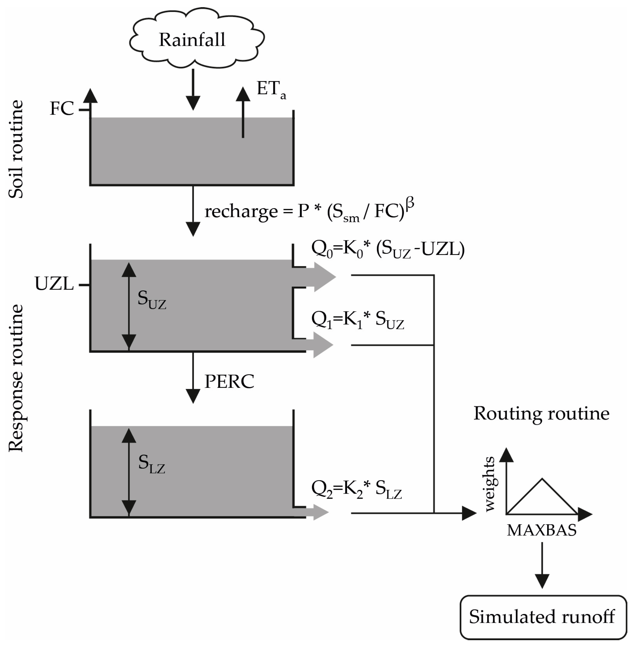
Figure 3.
Semilog plots showing MC hydrographs of simulated (black line) and observed (grey filled area) specific discharge. Panels show observed and simulated discharge from calibrations using rain gauge data (top); the non-bias corrected data (second); quantile mapped (QM) bias corrected data (third); model based bias correction (ModB) bias corrected data (fourth) and combined QM + ModB bias corrected data (bottom).
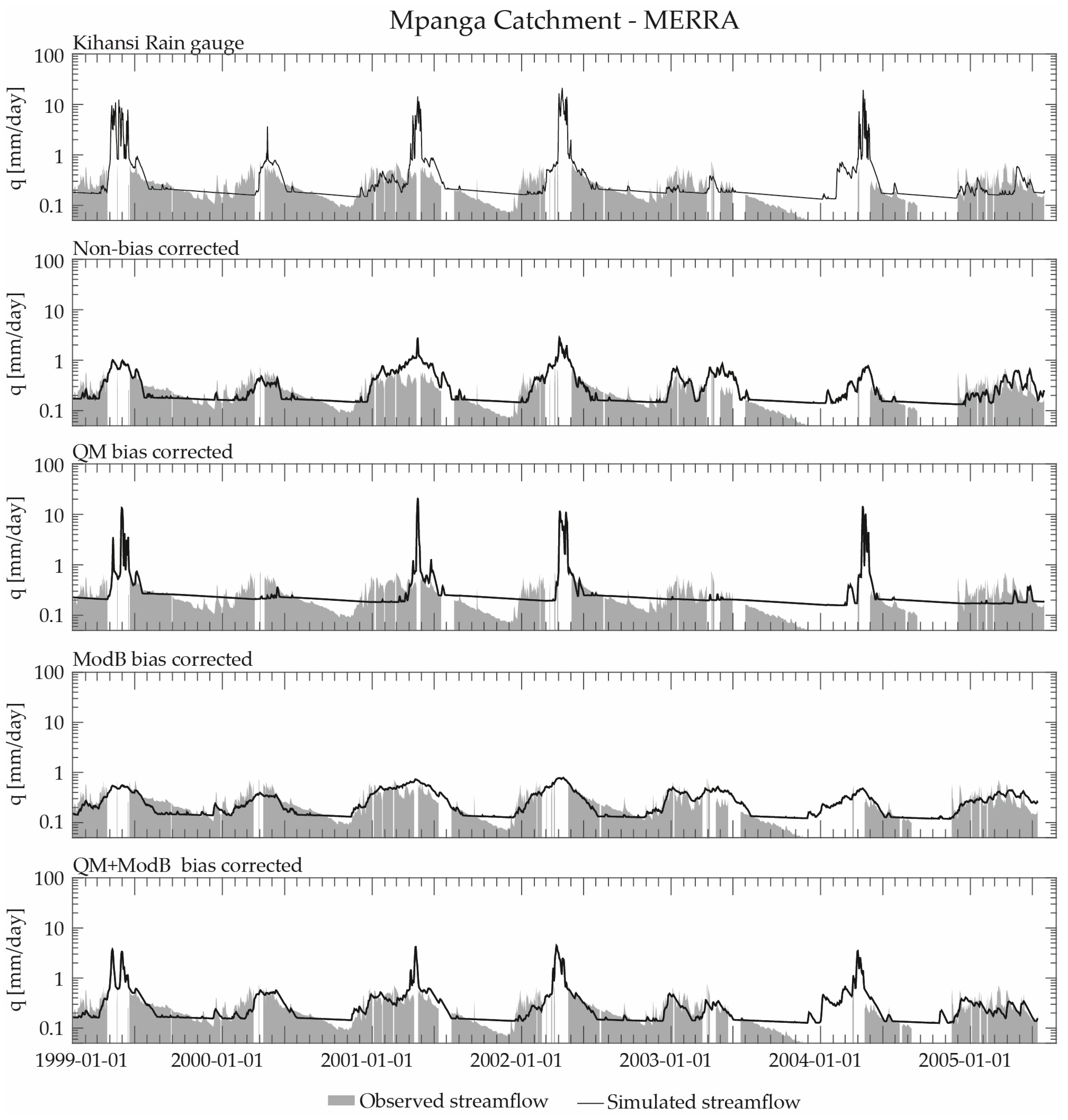
Figure 4.
Semilog plots showing KC hydrographs of simulated (black line) and observed (grey filled area) specific discharge. Panels show observed and simulated discharge from calibrations using rain gauge data (top); the non-bias corrected data (second); quantile mapped (QM) bias corrected data (third); model based bias correction (ModB) bias corrected data (fourth) and combined QM + ModB bias corrected data (bottom).
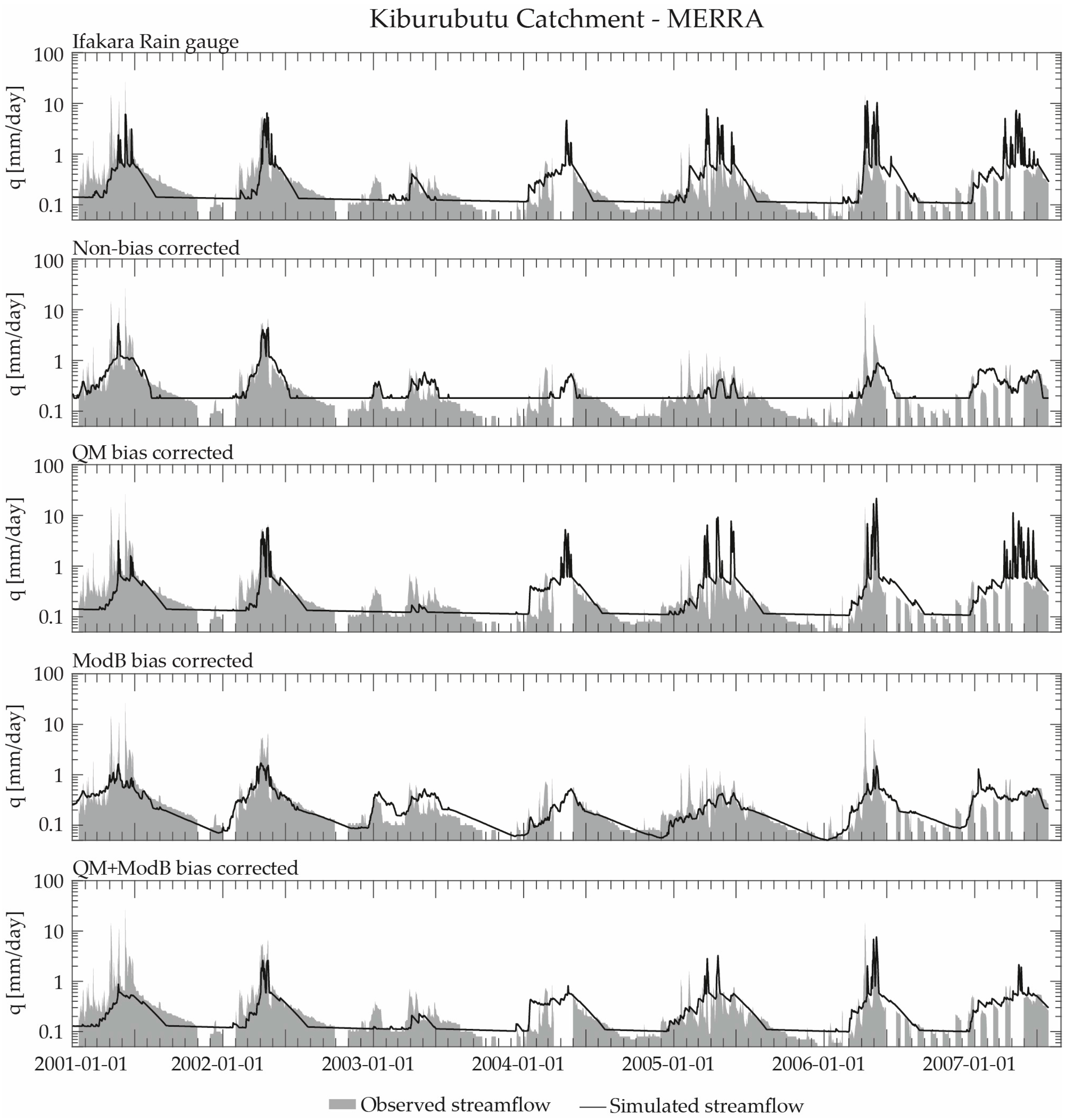

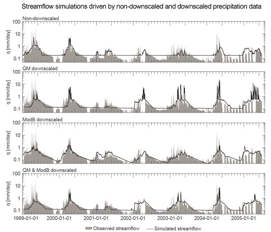
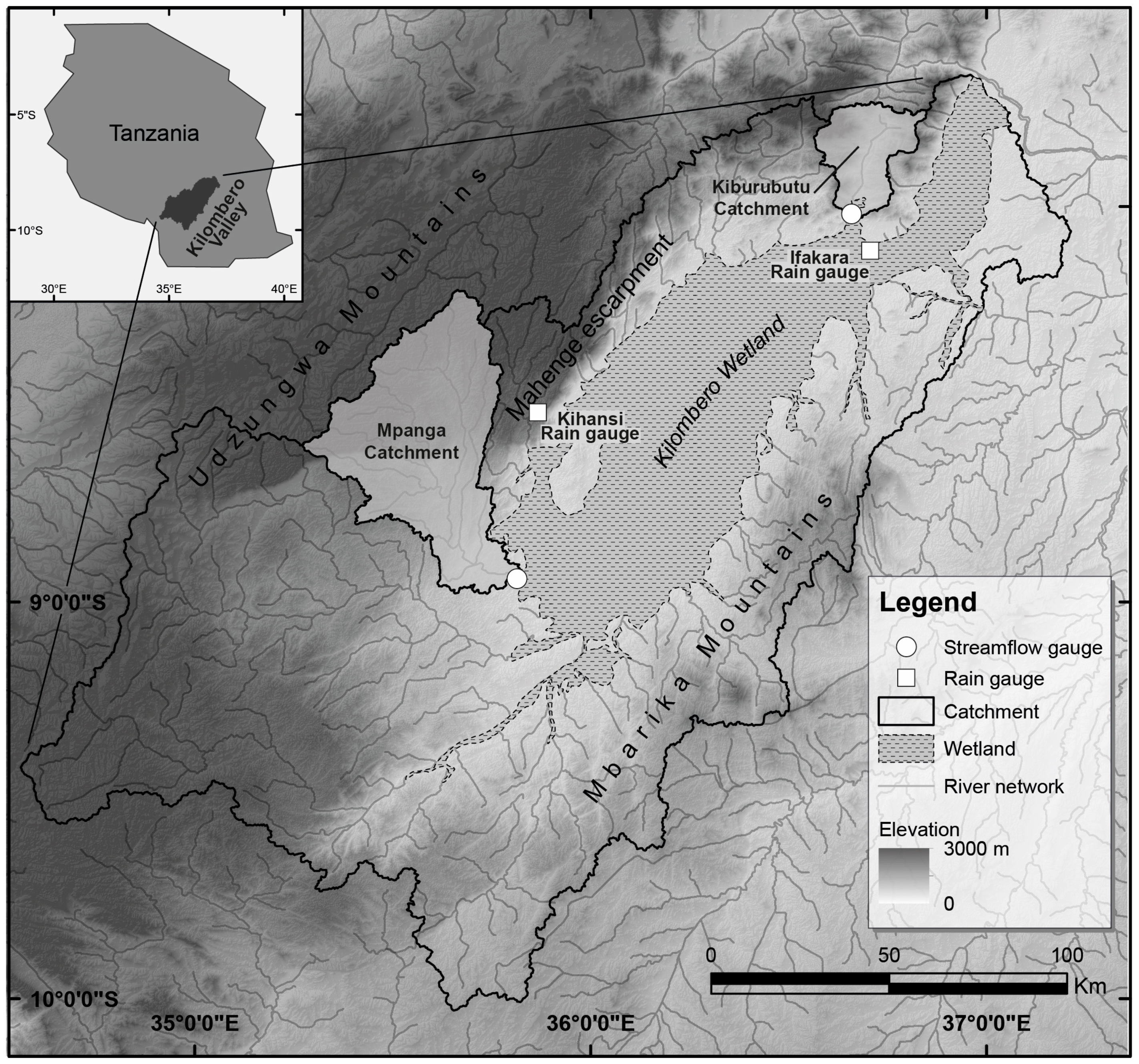
Table 1.
Characteristics of the global precipitation datasets considered in this study.
| Product | Type | Spatial Resolution | Spatial Coverage | Temporal Coverage | Temporal Resolution | n * | Reference |
|---|---|---|---|---|---|---|---|
| CMORPH | Satellite | 0.25° × 0.25° | 60 N–60 S | 1998–present | 0.5 h | 9;4 | [20] |
| TRMMv7 | Satellite | 0.25° × 0.25° | 50 N–50 S | 1998–present | 3 h | 9;4 | [41] |
| CFSR | Reanalysis | 0.50° × 0.50° | 90 N–90 S | 1979–present | 6 h | 7;4 | [22] |
| ERA-i | Reanalysis | 0.75° × 0.75° | 90 N–90 S | 1979–present | 6 h | 4;2 | [42] |
| MERRA | Reanalysis | 0.67° × 0.50° | 90 N–90 S | 1979–present | 1 h | 6;2 | [43] |
| CRU | Interpolated | 0.50° × 0.50° | 90 N–90 S | 1901–2014 | Monthly | 4;2 | [21] |
| GPCC | Interpolated | 0.50° × 0.50° | 90 N–90 S | 1900–2013 | Monthly | 4;2 | [44] |
| UDEL | Interpolated | 0.50° × 0.50° | 90 N–90 S | 1900–2014 | Monthly | 4;2 | [45] |
* n is the number of grid points that at least partially covered the catchment and thus were used for constructing precipitation time series. The first value is for MC, the second for KC. No pixel was completely within the catchment border for either catchment.
Table 2.
Parameter ranges for GAP optimization of streamflow simulations in HBV-light.
| Parameter | Min | Max |
|---|---|---|
| FC | 100 | 1000 |
| LP | 0 | 1 |
| β | 1 | 5 |
| PERC | 0 | 6 |
| UZL | 0 | 70 |
| K0 | 0.1 | 0.5 |
| K1 | 0.01 | 0.2 |
| K2 | 5E-07 | 0.1 |
| MAXBAS | 1 | 2.5 |
| PCORR * | 0.6 | 2 |
* Time-invariant correction factor as a multiplier on precipitation input.
Table 3.
Performance scores for MC discharge simulations. Performance is shown as Reff,log, R2, Ve, and RMSE values for each bias correction technique considered.
Table 3.
Performance scores for MC discharge simulations. Performance is shown as Reff,log, R2, Ve, and RMSE values for each bias correction technique considered.
| Mpanga Catchment | ||||||||||||
|---|---|---|---|---|---|---|---|---|---|---|---|---|
| GDP | Reff,log | R2 | Ve | RMSE | Reff,log | R2 | Ve | RMSE | ||||
| CFSR | Non- | bias corrected | 0.33 | 0.23 | 0.96 | 0.28 | ModB | bias corrected | 0.43 | 0.40 | 1.00 | 0.26 |
| ERAi | 0.53 | 0.48 | 0.96 | 0.23 | 0.53 | 0.50 | 0.96 | 0.23 | ||||
| MERRA | 0.38 | 0.44 | 0.94 | 0.29 | 0.61 | 0.58 | 0.99 | 0.22 | ||||
| CMORPH | 0.41 | 0.32 | 0.95 | 0.27 | 0.41 | 0.33 | 0.95 | 0.27 | ||||
| TRMMv7 | 0.45 | 0.36 | 1.00 | 0.27 | 0.51 | 0.42 | 0.99 | 0.24 | ||||
| Ensemble | 0.55 | 0.49 | 0.97 | 0.23 | 0.56 | 0.53 | 0.99 | 0.23 | ||||
| Rain gauge | 0.12 | 0.14 | 0.94 | 0.36 | 0.47 | 0.34 | 0.97 | 0.25 | ||||
| CRU * | 0.27 | 0.17 | 0.98 | 0.30 | 0.30 | 0.20 | 0.96 | 0.29 | ||||
| GPCC * | 0.29 | 0.23 | 0.99 | 0.30 | 0.32 | 0.24 | 0.97 | 0.29 | ||||
| UDEL * | 0.35 | 0.25 | 0.99 | 0.28 | 0.45 | 0.37 | 0.99 | 0.25 | ||||
| CFSR | QM | bias corrected | 0.22 | 0.18 | 0.96 | 0.33 | QM + ModB | bias corrected | 0.53 | 0.40 | 0.98 | 0.23 |
| ERAi | 0.18 | 0.16 | 0.91 | 0.35 | 0.54 | 0.41 | 0.98 | 0.23 | ||||
| MERRA | 0.05 | 0.08 | 1.00 | 0.33 | 0.52 | 0.45 | 0.98 | 0.23 | ||||
| CMORPH | 0.35 | 0.22 | 1.00 | 0.28 | 0.51 | 0.40 | 0.98 | 0.23 | ||||
| TRMMv7 | 0.19 | 0.15 | 0.91 | 0.35 | 0.51 | 0.42 | 0.98 | 0.24 | ||||
| Ensemble | 0.19 | 0.16 | 0.91 | 0.35 | 0.50 | 0.36 | 0.98 | 0.24 | ||||
| GPCC * | DP | bias corrected | 0.34 | 0.19 | 0.99 | 0.29 | DP + ModB | bias corrected | 0.37 | 0.23 | 0.97 | 0.28 |
| CRU * | 0.36 | 0.24 | 0.97 | 0.28 | 0.38 | 0.27 | 0.95 | 0.28 | ||||
| UDEL * | 0.46 | 0.32 | 0.96 | 0.27 | 0.52 | 0.44 | 1.00 | 0.24 | ||||
* Monthly products.
Table 4.
Performance scores for MC discharge simulations. Performance is shown as Reff,log values for each bias correction technique considered.
Table 4.
Performance scores for MC discharge simulations. Performance is shown as Reff,log values for each bias correction technique considered.

Table 5.
Performance scores for KC discharge simulations. Performance is shown as Reff,log, R2, Volume Error (Vol. Err.), and RMSE values for each bias correction technique considered.
Table 5.
Performance scores for KC discharge simulations. Performance is shown as Reff,log, R2, Volume Error (Vol. Err.), and RMSE values for each bias correction technique considered.
| Kiburubutu Catchment | ||||||||||||
|---|---|---|---|---|---|---|---|---|---|---|---|---|
| GDP | Reff,log | R2 | Vol. Err. | RMSE | Reff,log | R2 | Vol. Err. | RMSE | ||||
| CFSR | Non- | bias corrected | 0.38 | 0.01 | 0.78 | 0.26 | ModB | bias corrected | 0.41 | 0.01 | 0.74 | 0.25 |
| ERAi | 0.63 | 0.26 | 0.78 | 0.18 | 0.66 | 0.24 | 0.73 | 0.18 | ||||
| MERRA | 0.47 | 0.25 | 0.86 | 0.20 | 0.68 | 0.24 | 0.72 | 0.18 | ||||
| CMORPH | 0.56 | 0.08 | 0.79 | 0.23 | 0.62 | 0.10 | 0.68 | 0.20 | ||||
| TRMMv7 | 0.55 | 0.07 | 0.87 | 0.23 | 0.59 | 0.11 | 0.70 | 0.20 | ||||
| Ensemble | 0.63 | 0.19 | 0.80 | 0.19 | 0.67 | 0.22 | 0.73 | 0.19 | ||||
| Rain gauge | 0.52 | 0.25 | 0.96 | 0.23 | 0.59 | 0.21 | 0.78 | 0.20 | ||||
| CRU * | 0.42 | 0.09 | 0.97 | 0.29 | 0.57 | 0.12 | 0.70 | 0.21 | ||||
| GPCC * | 0.38 | 0.14 | 0.79 | 0.24 | 0.59 | 0.14 | 0.69 | 0.21 | ||||
| UDEL * | 0.47 | 0.12 | 0.86 | 0.23 | 0.64 | 0.16 | 0.71 | 0.19 | ||||
| CFSR | QM | bias corrected | 0.41 | 0.07 | 0.92 | 0.27 | QM + ModB | bias corrected | 0.53 | 0.12 | 0.71 | 0.20 |
| ERAi | 0.49 | 0.14 | 0.91 | 0.27 | 0.59 | 0.20 | 0.79 | 0.20 | ||||
| MERRA | 0.40 | 0.07 | 0.96 | 0.29 | 0.53 | 0.12 | 0.75 | 0.21 | ||||
| CMORPH | 0.44 | 0.05 | 0.92 | 0.27 | 0.51 | 0.08 | 0.74 | 0.22 | ||||
| TRMMv7 | 0.45 | 0.04 | 0.98 | 0.29 | 0.52 | 0.04 | 0.77 | 0.23 | ||||
| Ensemble | 0.48 | 0.07 | 0.91 | 0.29 | 0.56 | 0.06 | 0.83 | 0.23 | ||||
| GPCC * | DP | bias corrected | 0.51 | 0.20 | 0.96 | 0.24 | DP + ModB | bias corrected | 0.59 | 0.12 | 0.82 | 0.22 |
| CRU * | 0.51 | 0.13 | 0.99 | 0.26 | 0.57 | 0.18 | 0.83 | 0.21 | ||||
| UDEL * | 0.56 | 0.24 | 0.99 | 0.23 | 0.63 | 0.23 | 0.82 | 0.19 | ||||
* Monthly products.
Table 6.
Performance scores for KC discharge simulations. Performance is shown as Reff,log values for each bias correction technique considered.
Table 6.
Performance scores for KC discharge simulations. Performance is shown as Reff,log values for each bias correction technique considered.

© 2017 by the authors. Licensee MDPI, Basel, Switzerland. This article is an open access article distributed under the terms and conditions of the Creative Commons Attribution (CC BY) license (http://creativecommons.org/licenses/by/4.0/).
Share and Cite
MDPI and ACS Style
Koutsouris, A.J.; Seibert, J.; Lyon, S.W. Utilization of Global Precipitation Datasets in Data Limited Regions: A Case Study of Kilombero Valley, Tanzania. Atmosphere 2017, 8, 246. https://doi.org/10.3390/atmos8120246
AMA Style
Koutsouris AJ, Seibert J, Lyon SW. Utilization of Global Precipitation Datasets in Data Limited Regions: A Case Study of Kilombero Valley, Tanzania. Atmosphere. 2017; 8(12):246. https://doi.org/10.3390/atmos8120246
Chicago/Turabian StyleKoutsouris, Alexander J., Jan Seibert, and Steve W. Lyon. 2017. "Utilization of Global Precipitation Datasets in Data Limited Regions: A Case Study of Kilombero Valley, Tanzania" Atmosphere 8, no. 12: 246. https://doi.org/10.3390/atmos8120246
Note that from the first issue of 2016, this journal uses article numbers instead of page numbers. See further details here.