Urban Roughness Estimation Based on Digital Building Models for Urban Wind and Thermal Condition Estimation—Application of the SkyHelios Model


Abstract
:1. Introduction
2. Methods
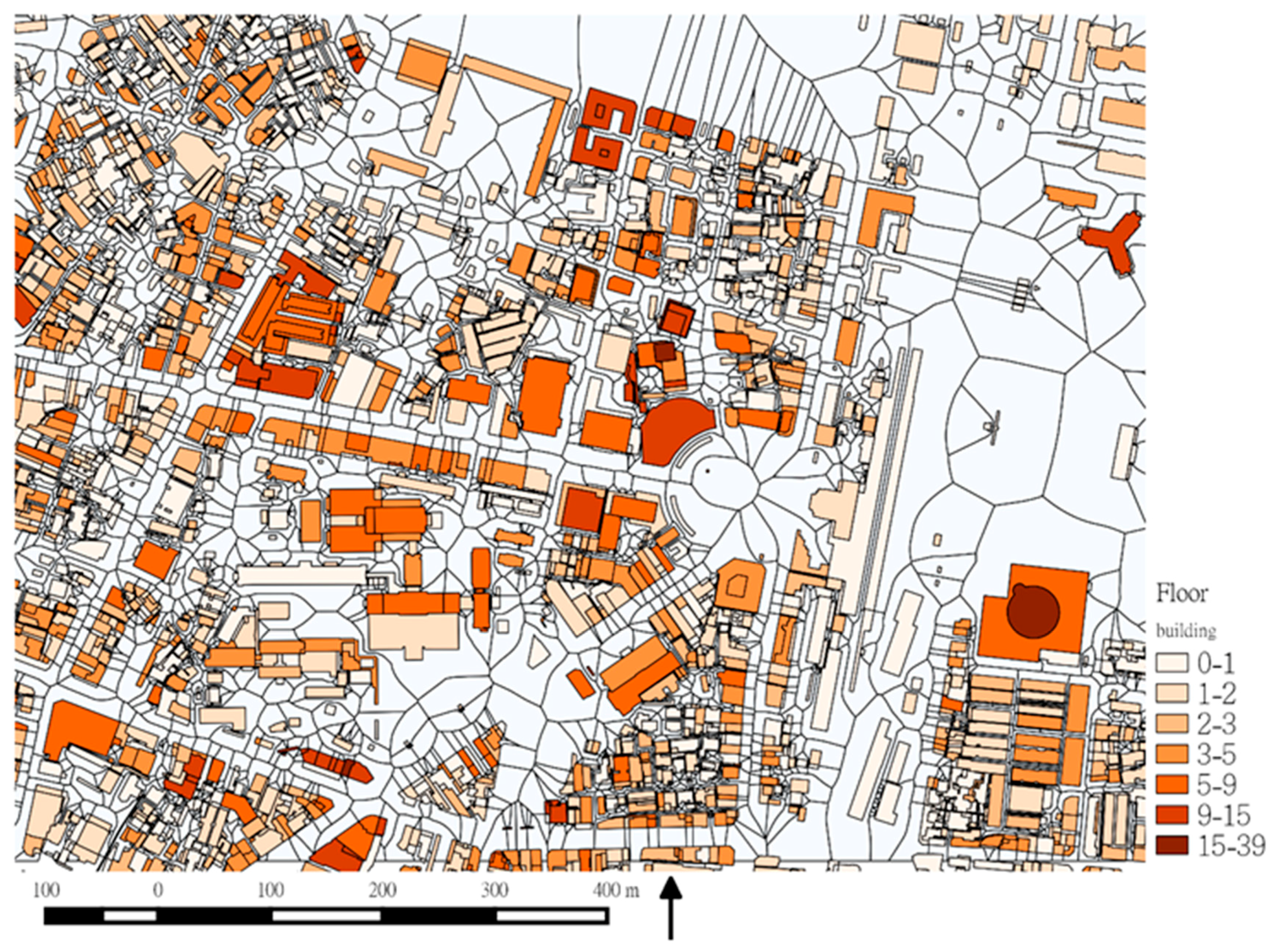
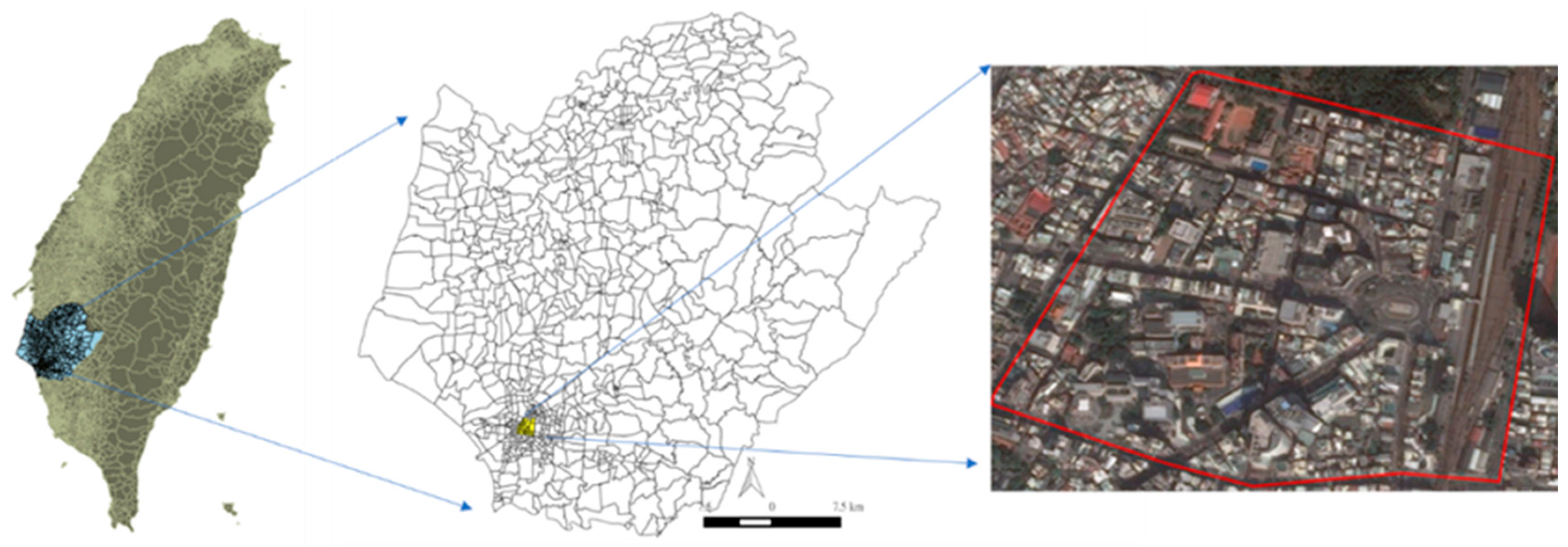
2.1. Study Area
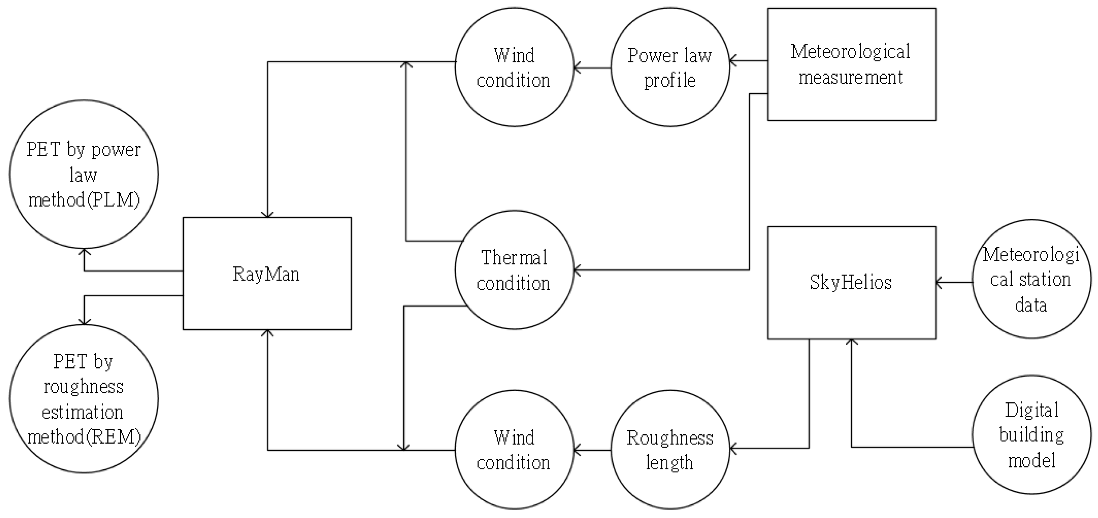
2.2. Research Structure
2.3. Local Roughness Estimation
2.4. Estimation of Wind Conditions
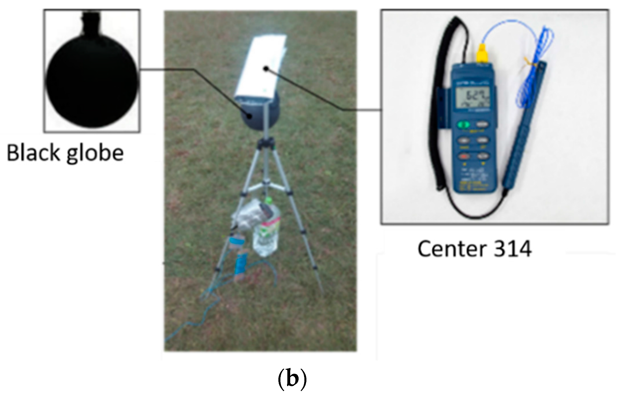
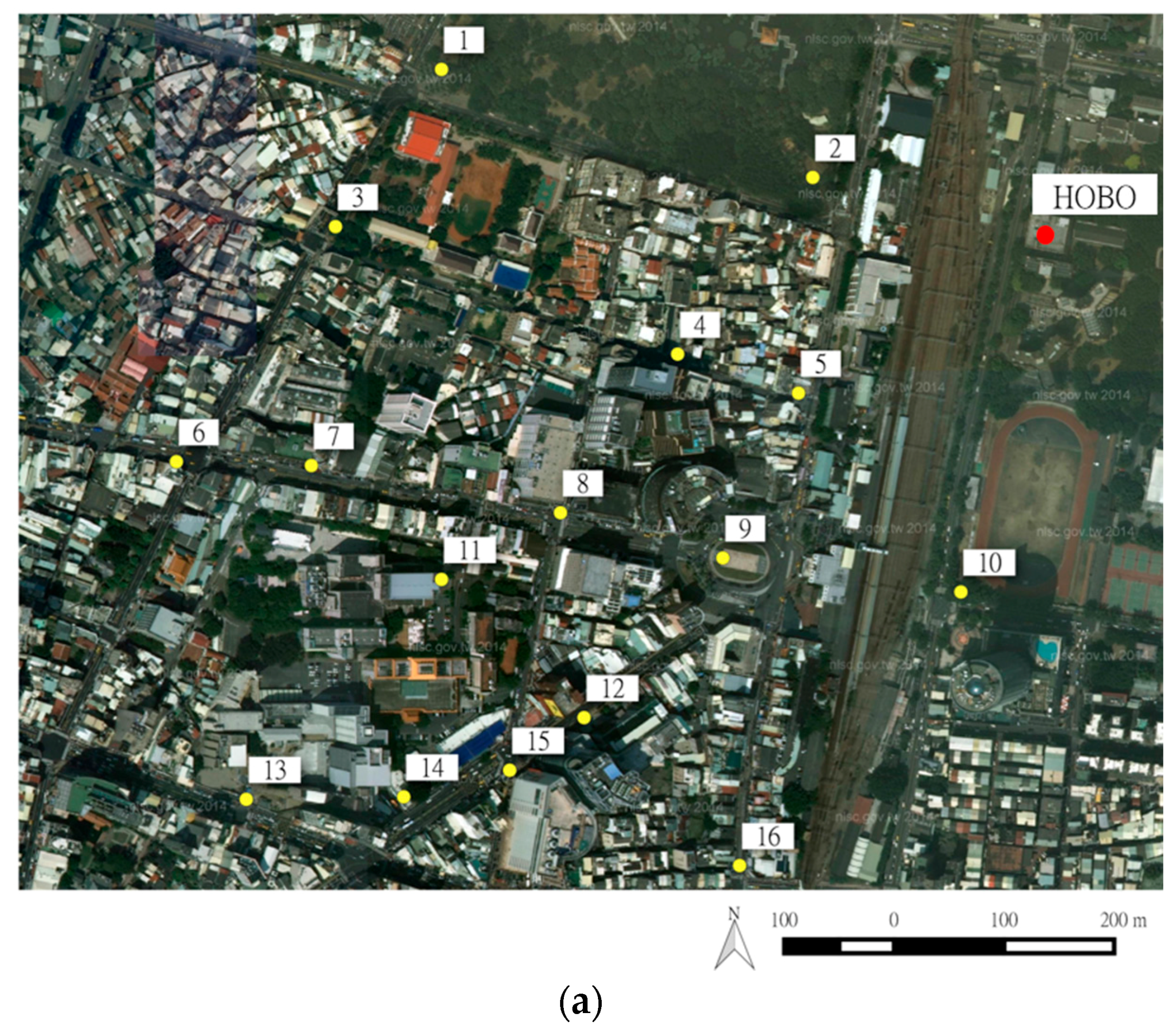
2.5. Meteorological Data Measurement Survey
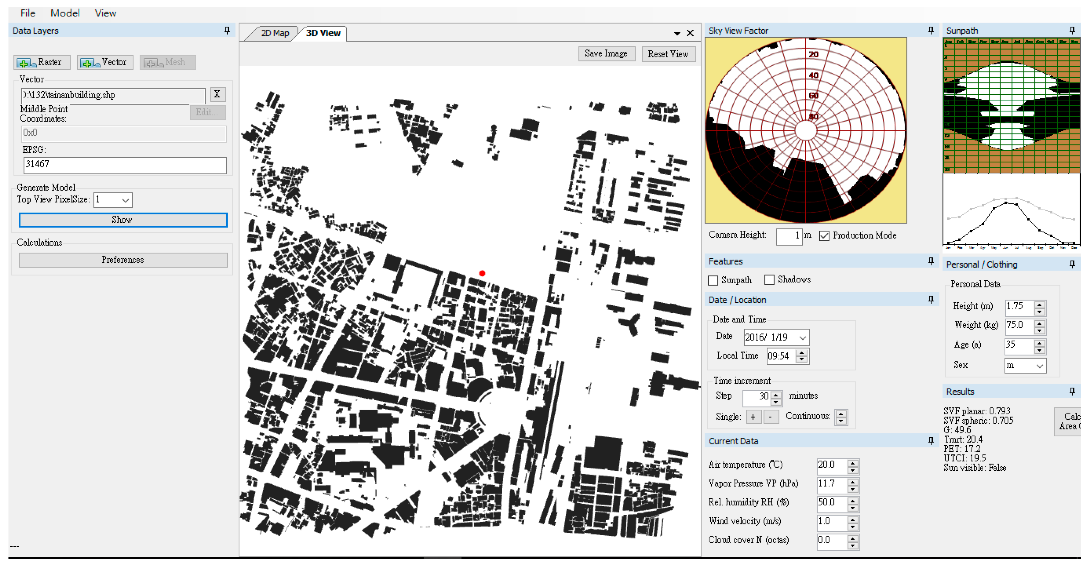
2.6. Estimation of Thermal Conditions
3. Results
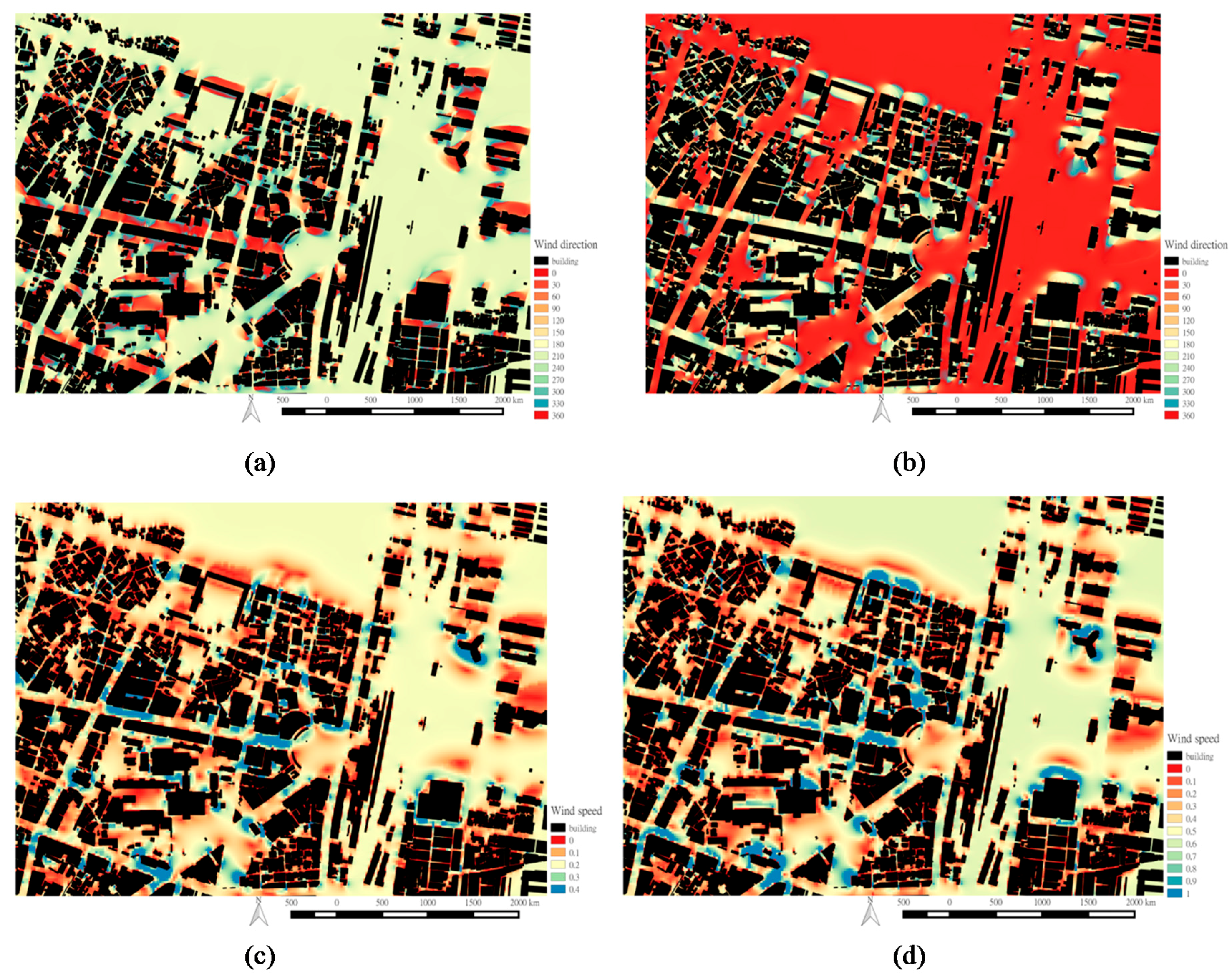
3.1. Wind Condition Mapping Based on Modeling
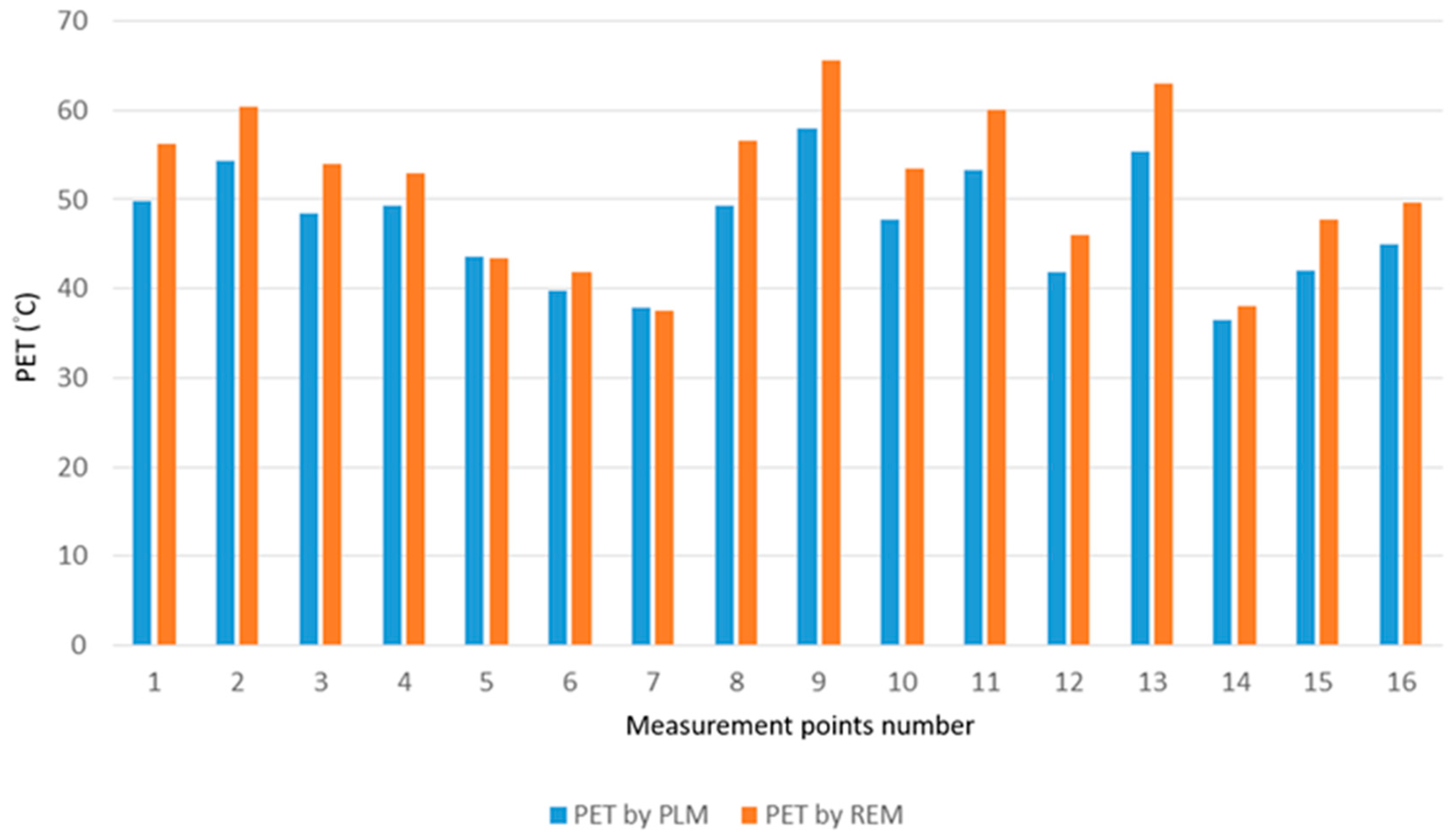
3.2. Thermal Environment Conditions Determined Using the PLM
3.3. Thermal Environment Conditions Determined Using the REM
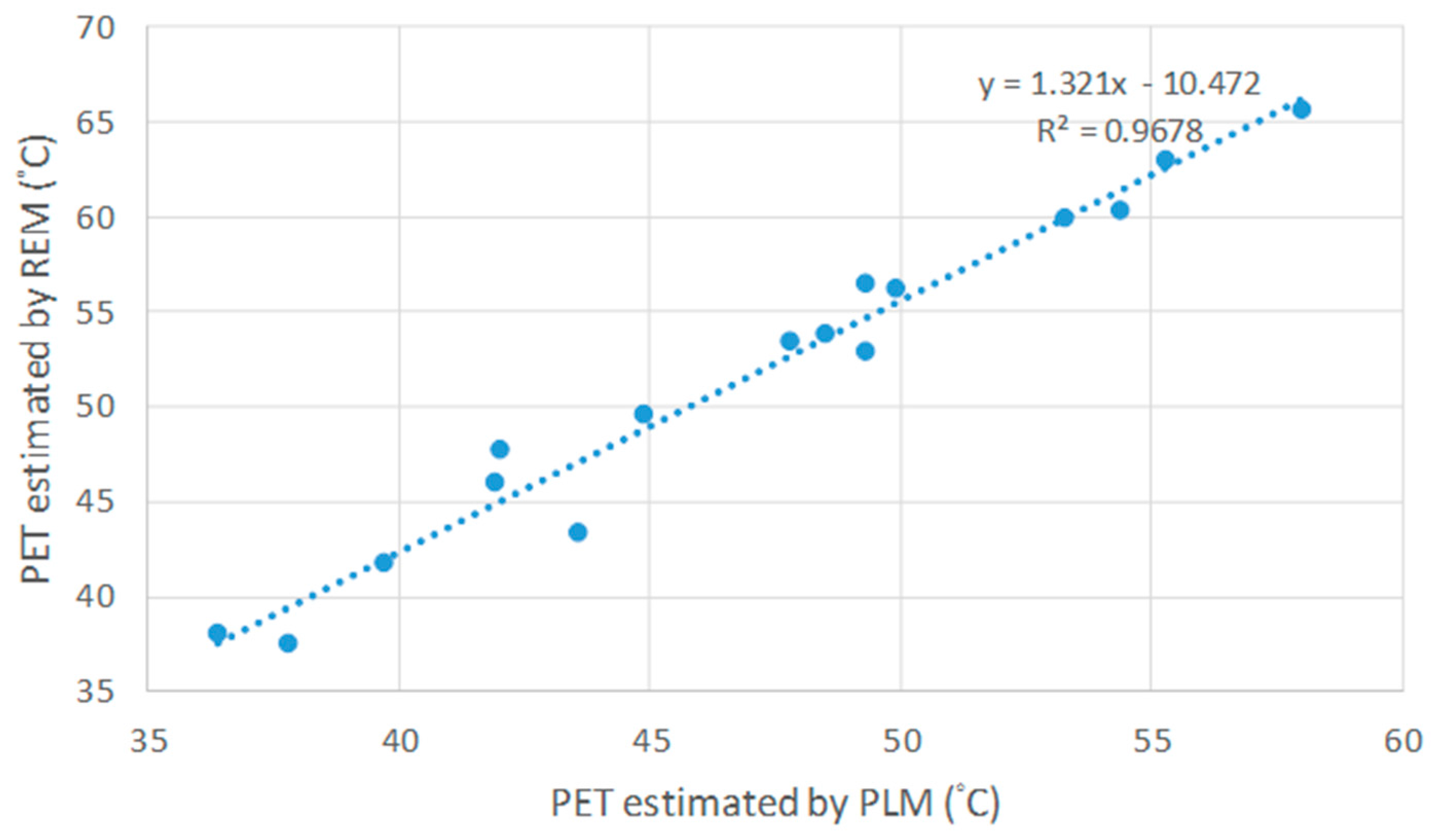
3.4. Correlation between Modeling and Measurements
4. Discussion
4.1. WS Difference Obtained Using the Two Methods
4.2. Main Findings and Comparison with Previous Studies
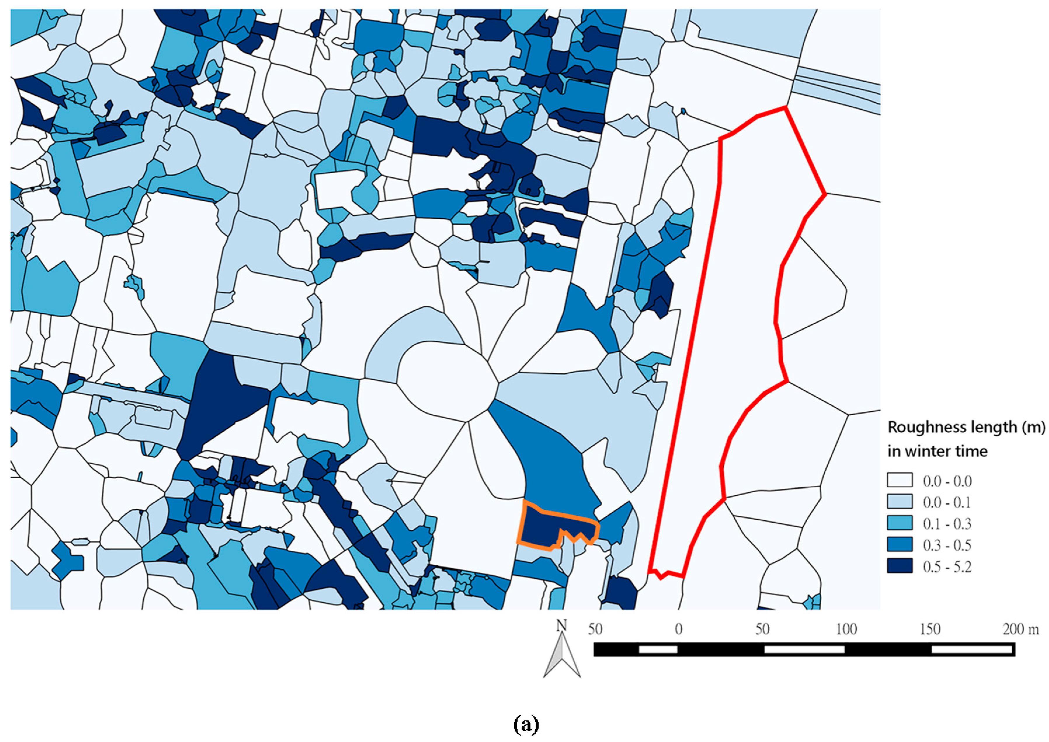
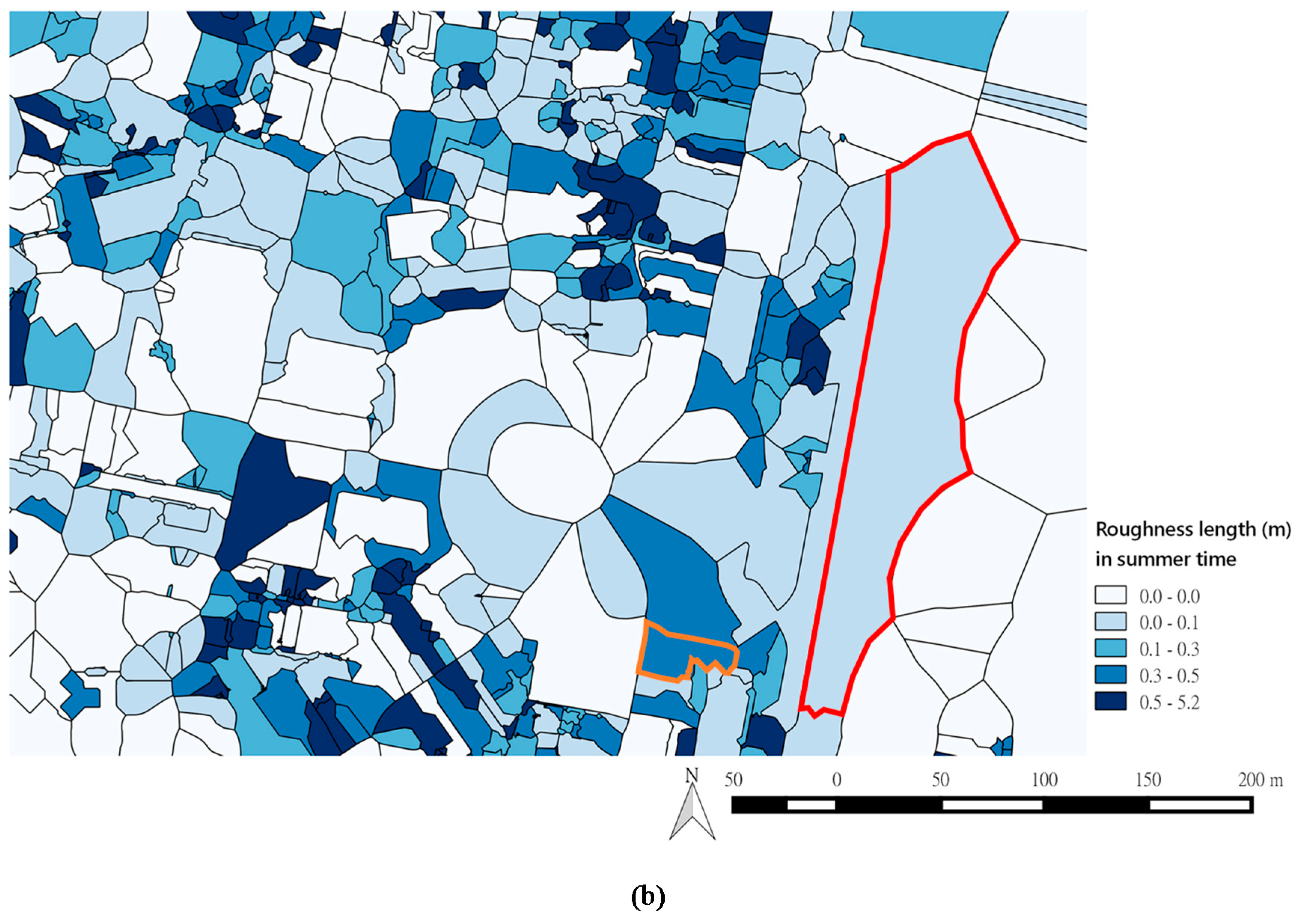
4.3. Differences in Roughness Length during Different Seasons
5. Conclusions
Acknowledgments
Author Contributions
Conflicts of Interest
References
- Wong, M.S.; Nichol, J.E.; To, P.H.; Wang, J. A simple method for designation of urban ventilation corridors and its application to urban heat island analysis. Build. Environ. 2010, 45, 1880–1889. [Google Scholar] [CrossRef]
- Atkinson, B.W. Numerical Modelling of Urban Heat-Island Intensity. Bound. Layer Meteorol. 2003, 109, 285–310. [Google Scholar] [CrossRef]
- Collier, C.G. The impact of urban area on weather. Q. J. R. Meteorol. Soc. 2006, 132, 1–25. [Google Scholar] [CrossRef]
- Müller, N.; Kuttler, W.; Barlag, A. Counteracting urban climate change: Adaptation measures and their effect on thermal comfort. Theor. Appl. Climatol. 2014, 115, 243–257. [Google Scholar] [CrossRef]
- Shishegar, N. Street design and urban microclimate: Analyzing the effects of street geometry and orientation on airflow and solar access in urban canyons. J. Clean Energy Technol. 2013, 1, 52–56. [Google Scholar] [CrossRef]
- Wever, N. Quantifying trends in surface roughness and the effect on surface WS observations. J. Geophys. Res. 2012, 117. [Google Scholar] [CrossRef]
- Gunturu, U.B.; Schlosser, C.A. Characterization of wind power resource in the United States. Atmos. Chem. Phys. 2012, 12, 9687–9702. [Google Scholar] [CrossRef] [Green Version]
- Van Hove, L.W.A.; Jacobs, C.M.J.; Heusinkveld, B.G.; Elbers, J.A.; van Driel, B.C.; Holtslag, A.A.M. Temporal and spatial variability of urban heat island and thermal comfort within the Rotterdam agglomeration. Build. Environ. 2015, 83, 91–103. [Google Scholar] [CrossRef]
- Faivre, R.D.; Colin, J.; Menenti, M. Evaluation of methods for aerodynamic roughness length retrieval from very high-resolution imaging LIDAR observations over the heihe basin in China. Remote Sens. 2017, 9, 63. [Google Scholar] [CrossRef]
- Ketterer, C.; Gangwisch, M.; Fröhlich, D.; Matzarakis, A. Comparison of selected approaches for urban roughness determination based on voronoi cells. Int. J. Biometeorol. 2016, 61, 189–198. [Google Scholar] [CrossRef] [PubMed]
- Matzarakis, A.; Endler, C. Climate change and thermal bioclimate in cities: Impacts and options for adaptation in Freiburg, Germany. Int. J. Biometeorol. 2010, 54, 479–483. [Google Scholar] [CrossRef] [PubMed]
- Grimmond, C.S.B.; King, T.S.; Roth, M.; Oke, T.R. Aerodynamic roughness of urban areas derived from wind observations. Bound. Layer Meteorol. 1998, 89, 1–24. [Google Scholar] [CrossRef]
- Houda, S.; Zemmouri, N.; Hasseine, A.; Athmani, R.; Belarbi, R.; Flow, U. A CFD model for simulating urban flow in complex. Online J. Sci. Technol. 2012, 2, 1–10. [Google Scholar]
- Fadl, M.S.; Karadelis, J. CFD Simulation for Wind Comfort and Safety in Urban Area: A Case Study of Coventry University Central Campus. Int. J. Archit. Eng. Constr. 2013, 2, 131–143. [Google Scholar] [CrossRef]
- Bruse, M. Die Auswirkungen Kleinskaliger Umweltgestaltung auf das Mikroklima. Entwicklung des Prognostischen Numerischen Modells ENVI-met zur Simulation der Wind-, Temperatur- und Feuchteverteilung in Städtischen Strukturen. Ph.D. Thesis, Ruhr-Universität Bochum, Bochum, Germany, 1999. [Google Scholar]
- Bruse, M.; Fleer, H. Simulating surface-plant-air interactions inside urban environments with a three dimensional numerical mode. Environ. Model. Softw. 1998, 13, 73–384. [Google Scholar] [CrossRef]
- Toparlar, Y.; Blocken, B.; Vos, P.; van Heijst, G.J.F.; Janssen, W.D.; van Hooff, T.; Montazeri, H.; Timmermans, H.J.P. CFD simulation and validation of urban microclimate: A case study for Bergpolder Zuid, Rotterdam. Build. Environ. 2015, 83, 79–90. [Google Scholar] [CrossRef]
- Blocken, B.; van der Hout, A.; Dekker, J.; Weiler, O. CFD simulation of wind flow over natural complex terrain: Case study with validation by field measurements for ria de ferrol, galicia, spain. J. Wind Eng. Ind. Aerodyn. 2015, 147, 43–57. [Google Scholar] [CrossRef]
- Chen, Y.C.; Lin, T.P.; Matzarakis, A. Comparison of mean radiant temperature from field experiment and modelling: A case study in Freiburg, Germany. Theor. Appl. Climatol. 2014, 118, 535–551. [Google Scholar] [CrossRef]
- Papadopoulou, M.; Raphael, B.; Smith, I.; Sekhar, C. Optimal Sensor Placement for Time-Dependent Systems: Application to Wind Studies around Buildings. J. Comput. Civ. Eng. 2015, 30. [Google Scholar] [CrossRef]
- Emeis, S. Vertical wind profiles over an urban area. Meteorol. Z. 2004, 13, 353–359. [Google Scholar] [CrossRef]
- Blocken, B. Computational fluid dynamics for urban physics: Importance, scales, possibilities, limitations and ten tips and tricks towards accurate and reliable simulations. Build. Environ. 2015, 91, 219–245. [Google Scholar] [CrossRef] [Green Version]
- Matzarakis, A.; Matuschek, O. Sky View Factor as a parameter in applied climatology—Rapid estimation by the SkyHelios Model. Meteorol. Z. 2011, 20, 39–45. [Google Scholar] [CrossRef]
- Höppe, P. The physiological equivalent temperature—A universal index for the biometeorological assessment of the thermal environment. Int. J. Biometeorol. 1999, 43, 71–75. [Google Scholar] [CrossRef] [PubMed]
- Lin, T.P.; Tsai, K.T.; Hwang, R.L.; Matzarakis, A. Quantification of the effect of thermal indices and sky view factor on park attendance. Landsc. Urban Plan. 2012, 107, 137–146. [Google Scholar] [CrossRef]
- Matuschek, O.; Matzarakis, A. Estimation of sky view factor in complex environment as a tool for applied climatological studies. In Proceedings of the Seventh Conference on Biometeorology, Meteorological Institute of the Albert-Ludwigs-Universität Freiburg Rep, Freiburg im Breisgau, Germany, 12–14 April 2010; Volume 20, pp. 534–539. [Google Scholar]
- Matzarakis, A.; Rutz, F.; Mayer, H. Modelling radiation fluxes in simple and complex environments—Application of the RayMan model. Int. J. Biometeorol. 2007, 51, 23–34. [Google Scholar] [CrossRef] [PubMed]
- Matzarakis, A.; Mayer, H.; Iziomon, M.G. Applications of a universal thermal index: Physiological equivalent temperature. Int. J. Biometeorol. 1999, 43, 76–84. [Google Scholar] [CrossRef] [PubMed]
- Lin, T.P.; Matzarakis, A. Tourism climate and thermal comfort in Sun Moon Lake, Taiwan. Int. J. Biometeorol. 2008, 52, 281–290. [Google Scholar] [CrossRef] [PubMed]
- Lettau, H. Note on aerodynamic roughness—Parameter estimation on the basis of roughness-element description. J. Appl. Meteorol. 1969, 8, 828–832. [Google Scholar] [CrossRef]
- Matzarakis, A.; Mayer, H. Mapping of urban air paths for planning in Munich. In Planning Applications of Urban and Building Climatology; The IFHP/ CIB-symposium: Berlin, Germany, 1992; Volume 16, pp. 13–22. [Google Scholar]
- Bottema, M.; Mestayer, P.G. Urban roughness mapping—Validation techniques and some first results. J. Wind Eng. Ind. Aerodyn. 1998, 74, 163–173. [Google Scholar] [CrossRef]
- Fröhlich, D. Development of a Microscale Model for the Thermal Environment in Complex Areas. Ph.D. Thesis, Albert-Ludwigs-University Freiburg, Freiburg im Breisgau, Germany, 2016. [Google Scholar]
- Röckle, R. Bestimmung der Strömungsverhältnisse im Bereich Komplexer Bebauungsstrukturen. Ph.D. Thesis, Technical University Darmstadt, Darmstadt, Germany, 1990. [Google Scholar]
- Macdonald, R.W. Modelling the mean velocity profile in the urban canopy layer. Bound. Layer Meteorol. 2000, 97, 25–45. [Google Scholar] [CrossRef]
- Bagal, N.; Pardyjak, E.; Brown, M. Improved Upwind Cavity Parameterizations for a Fast Response Urban Wind Model. In Proceedings of the 84th American Meteorological Society (AMS) Annual Meeting, Seattle, WA, USA, 13–16 January 2004; pp. 567–570. [Google Scholar]
- Pardyjak, E.R.; Brown, M.J.; Bagal, N. Improved Velocity Deficit Parameterizations for a Fast Response Urban Wind Model. In Proceedings of the 84th American Meteorological Society (AMS) Annual Meeting, Seattle, WA, USA, 13–16 January 2004; pp. 507–511. [Google Scholar]
- Singh, B.; Hansen, B.S.; Brown, M.J.; Pardyjak, E.R. Evaluation of the QUIC-URB fast response urban wind model for a cubical building array and wide building street canyon. Environ. Fluid Mech. 2008, 8, 81–312. [Google Scholar] [CrossRef]
- Mayer, H.; Höppe, P. Thermal comfort of man in different urban environments. Theor. Appl. Climatol. 1987, 38, 43–49. [Google Scholar] [CrossRef]
- Fröhlich, D.; Matzarakis, A. Modeling of changes in thermal bioclimate: Examples based on urban spaces in Freiburg, Germany. Theor. Appl. Climatol. 2013, 111, 547–558. [Google Scholar] [CrossRef]
- Gulyas, A.; Unger, J.; Matzarakis, A. Assessment of the microclimatic and human comfort conditions in a complex urban environment: Modelling and measurements. Build. Environ. 2006, 41, 1713–1722. [Google Scholar] [CrossRef]
- Peterson, E.W.; Hennessey, J.P., Jr. On the use of power laws for estimates of wind power potential. J. Appl. Meteorol. 1978, 17, 390–394. [Google Scholar] [CrossRef]
- Touma, J.S. Dependence of the wind profile power law on stability for various locations. J. Air Pollut. Control Assoc. 1977, 27, 863–866. [Google Scholar] [CrossRef]
- Lindén, J.; Holmer, B. Thermally induced wind patterns in the Sahelian city of Ouagadougou, Burkina Faso. Theor. Appl. Climatol. 2011, 105, 1–13. [Google Scholar] [CrossRef]
- Newman, J.F.; Klein, P.M. The Impacts of Atmospheric Stability on the Accuracy of WS Extrapolation Methods. Resources 2014, 3, 81–105. [Google Scholar] [CrossRef]
- Stewart, I.D.; Oke, T.R. Local Climate Zones for urban temperature studies. Bull. Am. Meteorol. Soc. 2012, 93, 1879–1900. [Google Scholar] [CrossRef]
- Kalyanapu, A.J.; Burian, S.J.; McPherson, T.N. Effect of land use-based surface roughness on hydrologic model output. J. Spat. Hydrol. 2009, 9, 51–71. [Google Scholar]
- Macdonald, R.W.; Griffiths, R.F.; Hall, D.J. An improved method for estimation of surface roughness of obstacle arrays. Atmos. Environ. 1998, 32, 1857–1864. [Google Scholar] [CrossRef]
- Holland, D.E.; Berglund, J.A.; Spruce, J.P.; McKellip, R.D. Derivation of effective aerodynamic surface roughness in urban areas from airborne Lidar terrain data. J. Appl. Meteorol. Climatol. 2008, 47, 2614–2626. [Google Scholar] [CrossRef]
- Bottema, M. Urban roughness modelling in relation to pollutant dispersion. Atmos. Environ. 1997, 31, 3059–3075. [Google Scholar] [CrossRef]
- Grimmond, C.S.B.; Oke, T.R. Aerodynamic properties of urban areas derived from analysis of surface form. J. Appl. Meteorol. Climatol. 1999, 38, 1262–1292. [Google Scholar] [CrossRef]
- Kwun, J.H.; Kim, Y.K.; Seo, J.W.; Jeong, J.H.; You, S.H. Sensitivity of MM5 and WRF mesoscale model predictions of surface winds in a typhoon to planetary boundary layer parameterizations. Nat. Hazards 2009, 51, 63–77. [Google Scholar] [CrossRef]
- Dudhia, J.; Bresch, J.F. A global version of the PSU-NCAR mesoscale model. Mon. Weather Rev. 2002, 130, 2989–3007. [Google Scholar] [CrossRef]
- Nielsen-Gammon, J.W.; McNider, R.T.; Angevine, W.M.; White, A.B.; Knupp, K. Mesoscale model performance with assimilation of wind profiler data: Sensitivity to assimilation parameters and network configuration. J. Geophys. Res. 2007, 112. [Google Scholar] [CrossRef]
- Childs, P.P.; Raman, S. Observations and numerical simulations of urban heat Island and sea breeze circulations over New York City. Pure Appl. Geophys. 2005, 162, 1955–1980. [Google Scholar] [CrossRef]


© 2017 by the authors. Licensee MDPI, Basel, Switzerland. This article is an open access article distributed under the terms and conditions of the Creative Commons Attribution (CC BY) license (http://creativecommons.org/licenses/by/4.0/).
Share and Cite
Chen, Y.-C.; Fröhlich, D.; Matzarakis, A.; Lin, T.-P. Urban Roughness Estimation Based on Digital Building Models for Urban Wind and Thermal Condition Estimation—Application of the SkyHelios Model. Atmosphere 2017, 8, 247. https://doi.org/10.3390/atmos8120247
Chen Y-C, Fröhlich D, Matzarakis A, Lin T-P. Urban Roughness Estimation Based on Digital Building Models for Urban Wind and Thermal Condition Estimation—Application of the SkyHelios Model. Atmosphere. 2017; 8(12):247. https://doi.org/10.3390/atmos8120247
Chicago/Turabian StyleChen, Yu-Cheng, Dominik Fröhlich, Andreas Matzarakis, and Tzu-Ping Lin. 2017. "Urban Roughness Estimation Based on Digital Building Models for Urban Wind and Thermal Condition Estimation—Application of the SkyHelios Model" Atmosphere 8, no. 12: 247. https://doi.org/10.3390/atmos8120247