Numerical Study on the Generation and Transport of Spume Droplets in Wind over Breaking Waves


1
Shanghai Institute of Applied Mathematics and Mechanics, Shanghai University, Shanghai 200072, China
2
Shanghai Key Laboratory of Mechanics in Energy Engineering, Shanghai 200072, China
3
Department of Mechanical Engineering, University of Minnesota, Minneapolis, MN 55455, USA
4
St. Anthony Falls Laboratory, University of Minnesota, Minneapolis, MN 55414, USA
*
Authors to whom correspondence should be addressed.
Atmosphere 2017, 8(12), 248; https://doi.org/10.3390/atmos8120248
Submission received: 31 October 2017
/
Revised: 28 November 2017
/
Accepted: 7 December 2017
/
Published: 12 December 2017
(This article belongs to the Section Biosphere/Hydrosphere/Land–Atmosphere Interactions)
Abstract
:Sea spray droplets play an important role in the momentum, heat and mass transfer in the marine atmospheric boundary layer. We have developed a new direct numerical simulation method to study the generation and transport mechanisms of spume droplets by wind blowing over breaking waves, with the wave breaking process taken into account explicitly. In this new computational framework, the air and water are simulated as a coherent system on fixed Eulerian grid with the density and viscosity varying with the fluid phase. The air-water interface is captured accurately using a coupled level-set and volume-of-fluid method. The trajectories of sea spray droplets are tracked using a Lagrangian particle-tracking method. The generation of droplets is captured by comparing the fluid particle velocity of water and the phase speed of the wave surface. From the simulation data, we obtain for the first time a detailed description of the instantaneous distribution of droplets at different stages of wave breaking. Furthermore, the time histories of the droplet number and its generation and disappearance rates are analyzed. Simulation cases with different parameters are performed to study the effects of wave age and wave steepness. The flow and droplet fields obtained from simulation provided a detailed physical picture of the problem of interest. It is found that plunging breakers generate more droplets than spilling breakers. Droplets are generated near the wave crest at young and intermediate wave ages, but at old wave ages, droplets are generated both near and behind the wave crest. It is also elucidated that the large-scale spanwise vortex induced by the wave plunging event plays an important role in suspending droplets. Our simulation result of the vertical profile of sea spray concentration is consistent with laboratory measurement reported in the literature.
1. Introduction
A large amount of sea spray droplets can be generated during wave breaking. Once sea spray droplets are generated, they are dispersed in the marine atmospheric boundary layer (MABL) and serve as an important component of the air-sea interface. Sea spray droplets enhance the interfacial heat flux [1,2], and small spray droplets suspended to high altitude affect the humidity and temperature profiles there through evaporation [3,4]. Moreover, the salt carried by sea spray droplets influences the radiative transfer and electro-optical properties of the MABL [4]. The investigation of the detailed flow physics associated with sea spray droplets, such as their turbulent transport by wind, the altitude they can reach and the duration they have for exchanging heat and moisture, is of great interest for developing climate and weather forecast models.
Sea spray droplets can be categorized into film droplets, jet droplets and spume droplets according to their generation processes [5,6,7,8,9,10,11,12]. Relevant to the present study, spume droplets are generated once the wind speed is high enough to provide sufficient surface shear stress to tear off the wave surface [13,14,15,16]. During measurements in the North Atlantic, Preobrazhenskii [17] observed spume droplets torn off by wind at the wave crest. He found that most droplets with µm are spume droplets. In laboratory experiments, Koga [18] observed the generation process of spume droplets and recorded droplets of µm. The radii of most spume droplets range from 10 µm–500 µm with the peak of the radius spectra centered at 100 µm [12,19,20,21]. Spume droplets of a larger radius can also be present. For example, Veron et al. [22] observed spume droplets of µm in laboratory experiments.
The effect of wind speed on the generation of spume droplets has been studied extensively [19,21,23,24,25,26]. Spume droplets are generated when , the wind speed at ten meters above the sea surface, is higher than 9–11 [12,14]. The wave age, i.e., the ratio of wave phase speed to the characteristic wind speed, also influences the generation of spume droplets [24,25,27,28]. While most spume droplets are generated at the wave crest at small wave ages, some can also be generated behind (with respect to the wave propagation direction) the wave crest at large wave ages [16].
The generation of sea spray and the effect of sea spray on the wind turbulence in extreme winds have drawn strong interests in the past few decades. Kudryavtsev and Makin [29] parameterized the effect of spume droplets on the turbulence mixing through stratification and found that the wind is accelerated and turbulence is suppressed due to the presence of sea spray droplets. Rastigejev et al. [30] pointed out that the concentration of spray increases rapidly with the wind speed at extreme winds, which results in a significant flow acceleration, compared to the wind without sea spray droplets. Rastigejev and Suslov [31] further found that the sea spray droplets suppress the turbulent momentum flux in the airflow. Wu et al. [32] pointed out that the effects of sea spray droplets on both the wind stress and heat flux are important in their air-sea interaction model. Zhang et al. [33] also showed that the sea spray droplets play a dominant role in the momentum transfer between air and water in their model of the marine atmospheric boundary at extreme winds. Rastigejev and Suslov [34] found that the evaporation of sea spray imposes significant mechanical and thermodynamic effects on the temperature, humidity and turbulent kinetic energy of the air in the lower atmosphere above the ocean. The aforementioned investigations of the effects of sea spray on the transport of momentum and temperature in extreme winds are based on parameterizations, while in laboratory experiments, the generation of sea spray droplets was studied. Ortiz-Suslow et al. [35,36] discovered that the concentration of spume droplets is proportional to at high wind speeds. Troitskaya et al. [37] pointed out that the breakup of large air pockets near the water surface is the major process that generates sea spray droplets at hurricane wind speeds.
Although the statistical properties of spume droplets have been studied through laboratory experiments [22,35,36], it is rather challenging to obtain the small-scale physics related to the detailed transport processes of droplets. Using numerical simulations, Richter and Sullivan [38,39] implemented a Lagrangian particle tracking (LPT) method to capture the motions of individual droplet particles in an idealized turbulent Couette flow. Based on the direct numerical simulation (DNS) of turbulence coupled with the LPT of droplet particles, they discovered that the ejection of airflow leads to accumulation of droplets. In a follow-up study, they found that droplets enhance the vertical heat flux by or greater [40]. Druzhinin et al. [41] conducted DNS coupled with the LPT method to study the wind over a stationary wavy bottom boundary. They found that the turbulence is suppressed as the wind speed increases.
The aforementioned numerical studies on the motion of droplets were not coupled to wave breaking explicitly. As summarized in many review papers, e.g., [42,43,44,45], substantial studies have been performed to investigate wave breaking. One of the major challenges in numerical simulations of wave breaking is the algorithm for capturing the air-water interface. The maker-and-cell method [46,47,48] was developed to capture the free surface in one-fluid simulations. In two-fluids simulations, interface tracking methods include, but are not limited to the level-set (LS) method [49,50,51], volume-of-fluid (VOF) method [52,53,54] and coupled LS-VOF (CLSVOF) [55,56,57] method. In general, the VOF method can conserve the mass of each phase of the fluids precisely, while the LS method captures the geometry of the air–water interface accurately.
In this paper, we present simulation results of the generation and transport of spume droplets in wave breaking. The CLSVOS method is used to capture the wave geometry. The LPT method is adopted for capturing the motions of sea spray droplets. With the use of the CLSVOF and LPT methods, the air, water and sea spray droplets can be solved on Eulerian grids. To the authors’ knowledge, this is one of the most advanced numerical models for simulating the transport of sea spray droplets with the breaking wave resolved directly. A kinematics-based criterion is applied for the generation of droplets. The effects of wave age and wave steepness on the generation and transport of droplets are analyzed.
2. Numerical Methods and Simulation Cases
2.1. Fluid Flow Solver
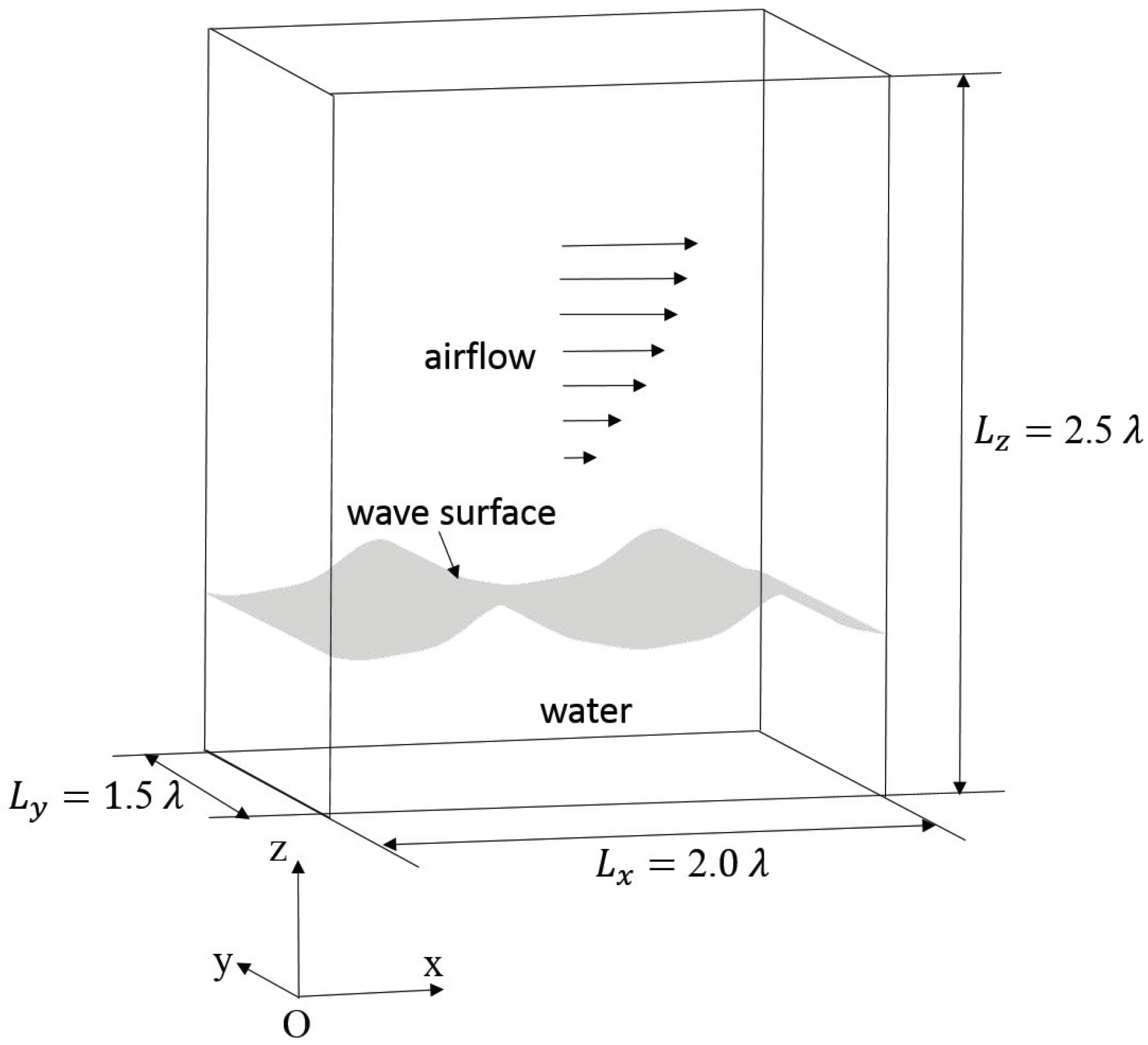
Figure 1 shows the computational domain and coordinate system used in the present study. Let x, y and z (or , and ) denote respectively the wave propagation, spanwise and vertical directions, with the corresponding velocity components denoted by u, v and w (or , and ), respectively. The mean velocity of the wind is in the same direction as the wave propagation. The computational domain is a box with the size , where is the wave length. The mean elevation of the water surface is set to . The mean depth of water and the mean height of air are and , respectively. The computational domain is discretized using a Cartesian grid system. The number of grid points is . The grid is evenly-spaced in the x- and y-directions. In the z-direction, the grid is refined near the wave surface between and , where the grid resolution is . The grid is stretched gradually to the bottom and top of the computational domain. Periodic boundary conditions are used in the x- and y-directions. We note here that the use of the periodic boundary condition is a common practice in simulations of breaking waves [58,59,60,61,62,63,64], because the non-periodic condition would substantially increase the computational cost. The no-slip condition is imposed at the bottom. At the top, the wind is driven by a constant shear stress in the streamwise direction, while shear-free () and impenetrable () conditions are prescribed for the spanwise and vertical velocity components, respectively. The initial flow field is fully-developed wind turbulence over prescribed steep waves. Following the practice of many previous two-fluid numerical simulations of wave breaking [58,59,60,61,62,63,64], the initial wave geometry is given by the analytical solution of the third-order Stokes wave as:
Here, is the wave surface elevation; is the initial wave amplitude; is the wave number; is the initial wave steepness; and is the phase speed of wave propagation, where is the angular frequency with g being the gravitational acceleration. The water velocities corresponding to the third-order Stokes wave are given as:
where is the water depth, which gives a dispersion parameter , representing a deep water condition.
To generate the initial flow field for simulating wind over breaking waves, the wave geometry and water velocities are prescribed using Equations (1) and (2), respectively, and the airflow is simulated using the algorithm introduced below. Once the airflow is fully developed, the time is set to and the two-fluid simulation of wave breaking starts.
The flows of air and water are simulated as a coherent system on a fixed Eulerian grid with the density and viscosity varying with the fluid phase. The dynamics of the two-fluid system are governed by the following continuity and momentum Equations,
Here, and are the densities and dynamic viscosities of the fluids; the LS function is defined as the signed distance to the air–water interface, for which the value is positive and negative in water and air, respectively; p is the pressure; is the strain rate tensor; and is the Kronecker delta tensor. Equations (3) and (4) are coupled to the LS function through the density and viscosity as [50]:
where the subscripts ‘a’ and ‘w’ denote air and water, respectively. The mollified step function is expressed as:
Here, is the smoothing thickness, with being the vertical grid size near the wave surface. Equation (4) is spatially discretized using the second-order central difference scheme. The second-order Runge–Kutta (RK2) method is used for the time integration. At each sub-step of the RK2 method, the divergence-free condition given by Equation (3) is enforced by using the fractional-step method [65] with a Poisson equation for the pressure solved by the PETSc (Portable, Extensible Toolkit for Scientific Computation) mathematic library [66].
The air-water interface is tracked by the CLSVOF method. The LS method solves the following advection equation of the LS function,
The VOF method is applied to keep the mass conserved for each phase of the fluids. The convection equation that governs the volume fraction is written as:
Here, is defined as the volume fraction of water in a cell. According to its definition, in the air, in the water and in cells with mixed air and water. Equations (8) and (9) are coupled using the method of Sussman and Puckett [55]. A more detailed description of the numerical method is given in Liu [57], Hu et al. [61] and Yang et al. [67].
2.2. Lagrangian Particle-Tracking Method
The LPT method has been used to simulate the motion of small particles with various sizes and geometries [68,69,70]. In the present study, we use the LPT method to track the sea spray droplets, which are treated as spherical particles. One-way coupling is considered here, with the feedback of droplets to the fluid flow and droplet-droplet interactions neglected, due to the low concentration of the droplets in the problem of interest. The kinematic equation of a spray droplet reads [71]:
where and are respectively the position and velocity of the droplet. The velocity of the droplet is governed by the following equation:
Here, is the fluid velocity at the position of the droplet, which may not be located exactly at any node of the Eulerian grid. Therefore, a fourth-order Lagrangian interpolation is used to calculate the fluid velocity at . The two terms on the right-hand side of Equation (11) are respectively the Stokes drag force and gravity, where is the vector of gravitational acceleration. The drag coefficient is given as [72]:
where is the droplet Reynolds number. This empirical equation of the drag coefficient is valid for droplets with [72], which is satisfied for sea spray droplets. Other forces exerted on a particle moving in fluid, such as the Basset history force, added mass term and Saffman lift force, are important if the densities of particle and fluid are of the same order [73]. However, the density ratio () in the present study is significantly higher than unity. As a result, only the Stokes drag force and gravity are considered in the present numerical framework. A second-order Adams–Bashforth scheme is used for the integration of Equations (10) and (11) in time.
2.3. Generation of Spume Droplets
In this study, we consider two groups of spume droplets, of which the radii are µm and 400 µm, respectively. At the beginning of the simulation, there are no droplets. During the simulation, we search grid points in the water phase to determine if a droplet is to be generated in the air at the next time step. To save computational time, only the grid points located one cell below the wave surface need to be searched. Let denote the velocity of a water parcel at at time step n. The position and velocity of this water parcel at time step are estimated as and , respectively, where is the right-hand side of Equation (4). If turns out to be located in the air phase at step , then a droplet is generated. The position and velocity of this droplet are given as:
The above droplet-generation method is based on the kinematics of air and water flows in breaking waves, i.e., spume droplets are generated if the fluid particle velocity at the water surface exceeds the wave phase speed. While it is desirable to prescribe the droplet initial location and ejection velocity based on experiment measurement, such data are currently unavailable [12,16]. In this study, we take advantage of the air-water coupled DNS that is capable of resolving the flow details in wave breaking and, thus, construct the above kinematics-based model for the mechanistic study of canonical problems. The physical meaning of the present kinematics-based model can be understood as a sea spray droplet is generated, if the velocity of a water parcel moves faster than the speed of the air-water interface, i.e., the phase speed of the wave. We remark here that the present kinematic criterion has limitations. Because the physical scale corresponding to the generation of sea spray droplets is much smaller than the present grid scale, the present model cannot address how the fluid parcels turn into droplets and what the radii of the droplets are. As a result, the droplets of different radii are generated at the same rate in the present study. It is important to study the transport of droplets of different radii systematically in the future. However, more measurement data on the initial location and ejection velocity of spray droplets of various sizes are needed. When a droplet falls back to the water phase, it is removed from the simulation.
2.4. Simulation Cases and Parameters
We have performed four simulation cases to study the motion of spume droplets over breaking waves. Table 1 summarizes the key parameters. The wave length is set to 5 m in all cases. The effect of the wave age is investigated through Cases A55, B55 and C55, in which is set to 3.7 (young wave), 12 (intermediate wave) and 27.7 (old wave), respectively. Here, c denotes the analytical solution of the phase speed of the third-order Stokes wave, and represents the friction velocity of wind. Plunging breakers are generated in these three cases by setting the initial wave steepness to . In Case A38, is smaller than the value in the other three cases, and spilling breakers are generated. Note that the wave phase speed c varies with the wave steepness . As a result, to keep the wave ages in Cases A38 and A55 the same, the wind speeds in these two cases differ slightly. In Table 1, we also summarize measured by Buckley and Veron [74] at the corresponding wave ages as an estimation of the wind speed. As shown, the wind speeds in Cases A55 and A35 are of practical interest, but those in Cases B55 and C55 are lower than the critical wind speed = 9–11 at which spume droplets are generated [12,14]. Cases B55 and C55 have relevance to the transport of sea spray droplets over swell-waves in the surf zone under low wind speeds. The wave period is used as the characteristic time scale for analyzing the results. The densities of air and water are set to the values at 1 atm and 20 °C. The realistic dynamic viscosities and under the same condition are also listed in the table. The value of the Reynolds number based on the realistic viscosity of air is . To perform DNS, we reduce the Reynolds number to by using an artificially lower dynamic viscosity of air, , for which the value is given in Table 1. We remark that the present work is the first simulation-based study on sea spray droplets in wind over waves, with the wave breaking process resolved explicitly. Unfortunately, the present computing power does not allow us to resolve the Kolmogorov scale of wind turbulence and the wave geometry simultaneously. While a realistic Reynolds number enabled by large-eddy simulation (LES) is more desirable, there are many challenging issues in LES, such as the subgrid-scale (SGS) modeling in air-water mixed flows and wall-layer modeling at the surfaces of breaking waves, which need substantial research. Therefore, it is more feasible to conduct DNS with a reduced Reynolds number. In the previous DNS of wave breaking without wind, it was observed that the wave geometry is not sensitive to the Reynolds number [63,64]. In the present study, an additional complexity is the strong wind shear that was not present in the previous DNS studies of wave breaking. Using the artificially high viscosity of air overestimates the viscous wind shear stress on the water, which tends to alter the wave geometry slightly. However, benefiting from the use of the high viscosity, the airflow can be resolved to the Kolmogorov scale. Meanwhile, the major events during wave breaking, such as wave plunging and water splash-up, can be captured in the simulation. Important features of wind turbulence in response to the wave breaking, such as airflow separation and the generation of large vortices, can also be observed. At the present very early stage in the numerical research on the complex subject of the transport of sea spray droplets in wave breaking, we focus our effort on developing the numerical framework. As a result, we leverage DNS, being a powerful research tool for mechanistic study without the use of ad hoc turbulence models [75]. The viscosity ratio between air and water is not altered, i.e., . The real viscosity of air is used for calculating the drag coefficient in Equation (11), so that the motions of droplets are captured correctly.
3. Results
We first demonstrate in Figure 2 representative snapshots of the three-dimensional field of droplets in Case A55 as an example of the evolution of droplets at different stages of wave breaking. As shown in Figure 2a, no droplet is present before the plunging event. When the wave front is steepened, droplets are generated near the wave crest (Figure 2b). More droplets are generated and suspended in air during the plunging events (Figure 2c). The wind sends some of the droplets far away from the wave surface at the late stage of wave breaking (Figure 2d). Note that due to the use of the periodic boundary condition in the streamwise direction, we essentially simulate a chain of breaking waves. The sea spray droplets shown in the figure are generated by breaking waves upstream of the boundary at an earlier time. The more detailed transport process of the sea spray droplets can be seen in the Supplementary Video S1.
Figure 3 shows the instantaneous streamwise profile of the droplet concentration and the projected positions of droplets in an x–z plane, together with the flow field, at different stages of wave breaking in Case A55. Here, is defined as:
where is the number of droplets in the interval between x and . In the simulation, the calculation of is simplified to:
where is the grid size in the x-direction. The value of is normalized by , where the reference droplet number is chosen as the maximal number of droplets of µm over all the time instances for all the cases. According to the definition of , the value of is between zero and one in all cases, where N is the instantaneous number of sea spray droplets. We use the same to normalize the results for droplets of µm, as well as the results in other cases, such that the number of droplets in different cases can be compared directly to illustrate the effects of wave age, wave steepness and droplet radius.
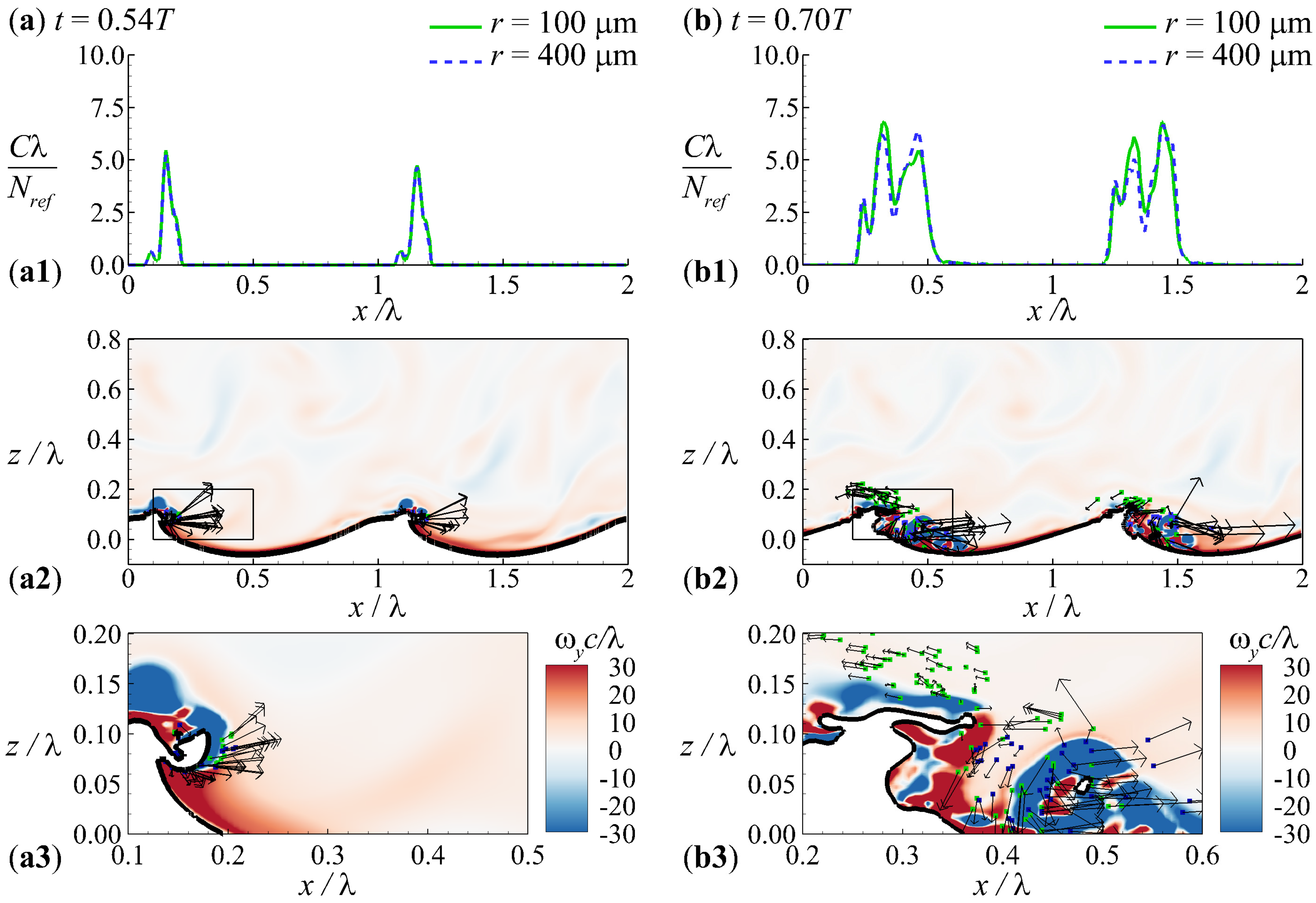
A sharp peak occurs in the horizontal profile of near each wave crest at (Figure 3(a1)), because droplets are generated at the wave crest when the wave front is steepened (Figure 3(a2)). The three-dimensional effect is not strong at the early stage of wave breaking, such that the projected positions of droplets collapse to the same location in the x–z plane. As a result, the real number of droplets is larger than what appears in Figure 3(a2,a3). Large negative spanwise vorticity is induced near the overturning jet, indicating the occurrence of a coherent spanwise vortex rotating in the counterclockwise direction (Figure 3(a3)). The spanwise vortex induces a positive vertical velocity in the downstream. Figure 3(b3) shows that when the spanwise vortex detaches from the wave surface at , the vertical motion of most droplets to the right of the vortex is upward. As a result, the profile of forms a bimodal shape within each wave length, with one peak located near the wave crest and the other in the downstream of the vortex (Figure 3(b1)). From the comparison between Figure 3(b1,c1), it is known that as the vortex moves far away from the wave crest, the peak of in the downstream of the vortex is flattened, because a large portion of the droplets falls back to the water.
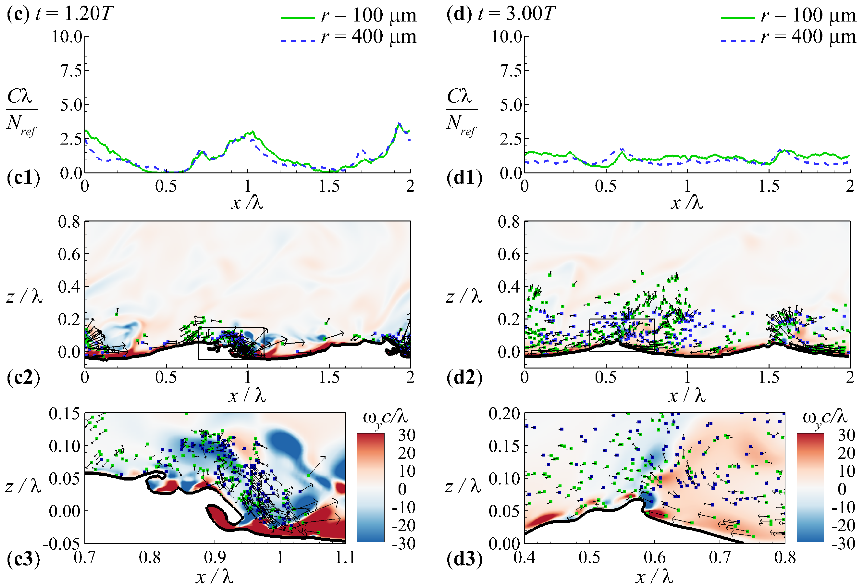
The first plunging event ends around , and then, another overturning jet is formed at (Figure 3(d2,d3)). The occurrence of successive splash-ups during plunging wave breaking has been reported in previous studies [58,60,62,63]. The sea spray droplets generated during the first wave plunging are transported downstream with the wind. Note that the sea spray droplets near are generated by the upstream wave, for which the crest is located near . Due to the use of the periodic boundary condition in the streamwise direction, these droplets leave the computational domain at and re-enter at . The generation and transport of droplets during the second plunging event are similar to those during the first plunging event. As shown in Figure 3(d2), a large number of droplets is generated near the tip of the jet. The second plunging event also induces a spanwise vortex (Figure 3(d3)), suspending the droplets in the downstream of it, which is evident from the bimodal shape of the profile of for droplets of µm (Figure 3(d1)). However, for droplets of µm, the peak of in the downstream of the vortex is absent here, indicating that the coherent vortex induced by the second plunging event is not sufficiently strong to suspend droplets with larger radii. Because the wind speed near the wave trough is low due to the airflow separation, the sea spray droplets near the wave surface are decelerated due to the wind drag. As a result, the vectors of these sea spray droplets point in the upstream direction. Note that the vectors show the relative velocity of sea spray droplets with respect to the wave phase speed (Figure 3(d3)).
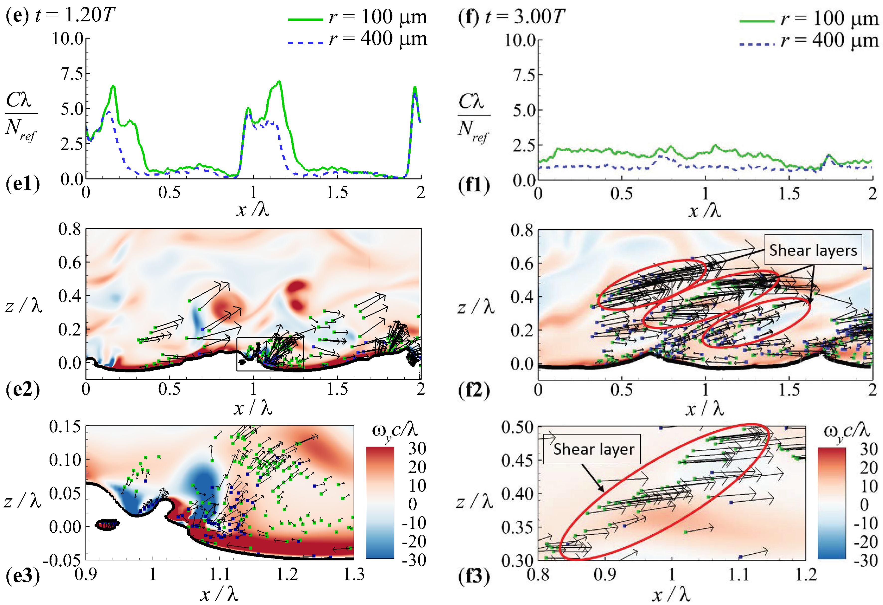
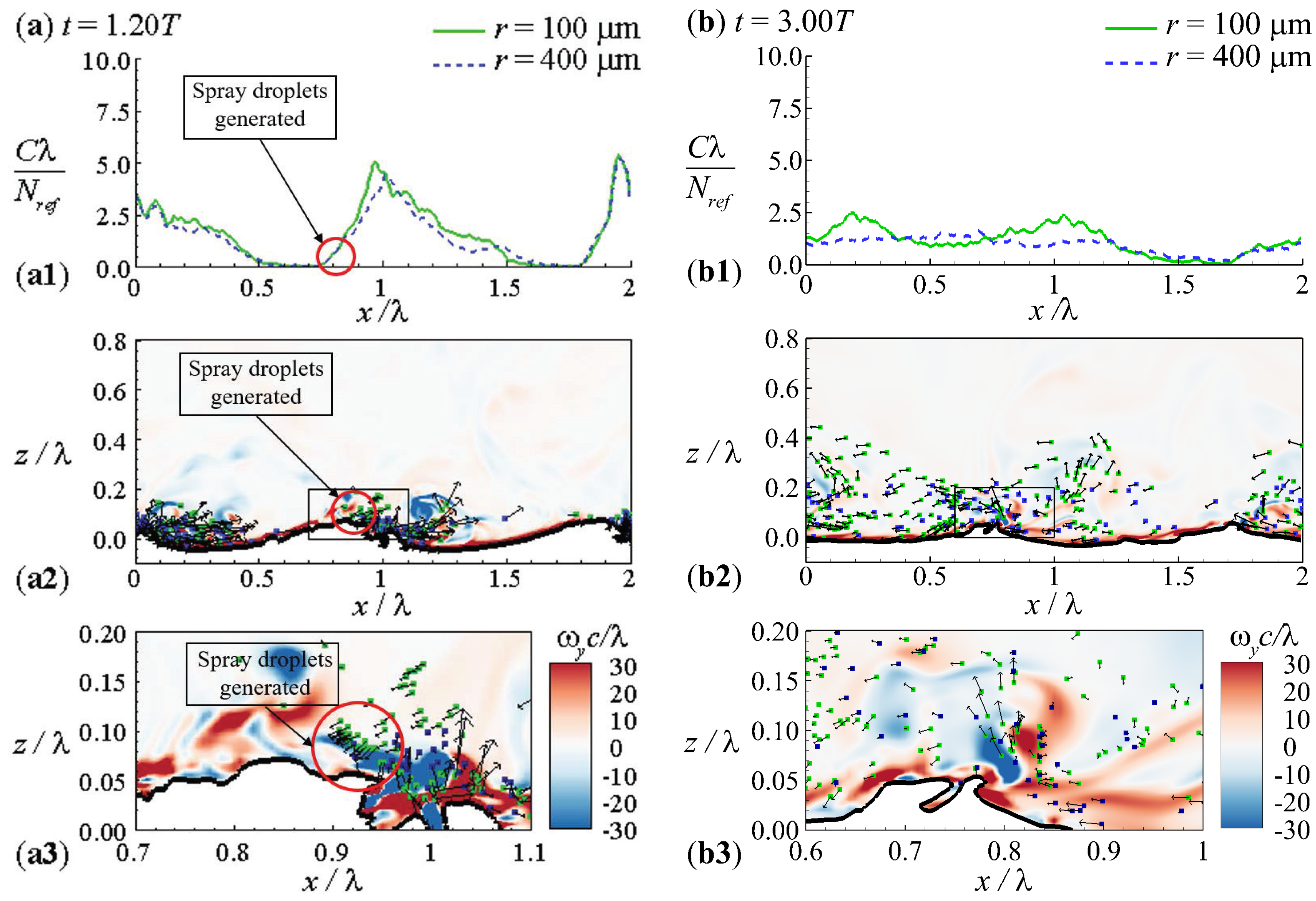
When the second overturning jet impinges the wave surface (Figure 3(e2,e3)), the generation of droplets becomes less active compared with that during the first plunging event, characterized by the decrease of near the wave crest (Figure 3(e1)). Furthermore, Figure 3(e2) shows that some of the droplets suspended during the first plunging event reach a high altitude of at .
At the late stage of wave breaking , the profile of is flatter than that during the first and second plunging events due to the convection of droplets in the horizontal direction. Airflow separation occurs over the wave crest, characterized by the shear layer shown in Figure 3(f2). Three shear layers can be observed from the figure. The first and third shear layers from left to right are attached to the wave crests near and 0.7, respectively. Due to the use of the periodic boundary condition, the first shear layer is broken into two parts in the figure. The mechanism underlying the second shear layer is not conclusive from the present simulation. We tracked the time history of the contours of the spanwise vorticity in this case and found that this shear layer is generated during wave plunging. Figure 3(d2) shows that at , a shear layer detaches from the wave crest and transports downstream. This detached shear layer is still present at , but the magnitude of vorticity is smaller than at . The separated air flows upward, which tends to suspend the droplets. As a result, the droplets are accumulated along the shear layer, with their vertical velocity being positive. There are more droplets of µm than those of µm near the shear layer (Figure 3(f3)), indicating that small droplets follow the airflow better than large droplets, which is as expected and is consistent with the conclusion drawn from previous studies on the motion of solid particles in other types of flows [76,77].
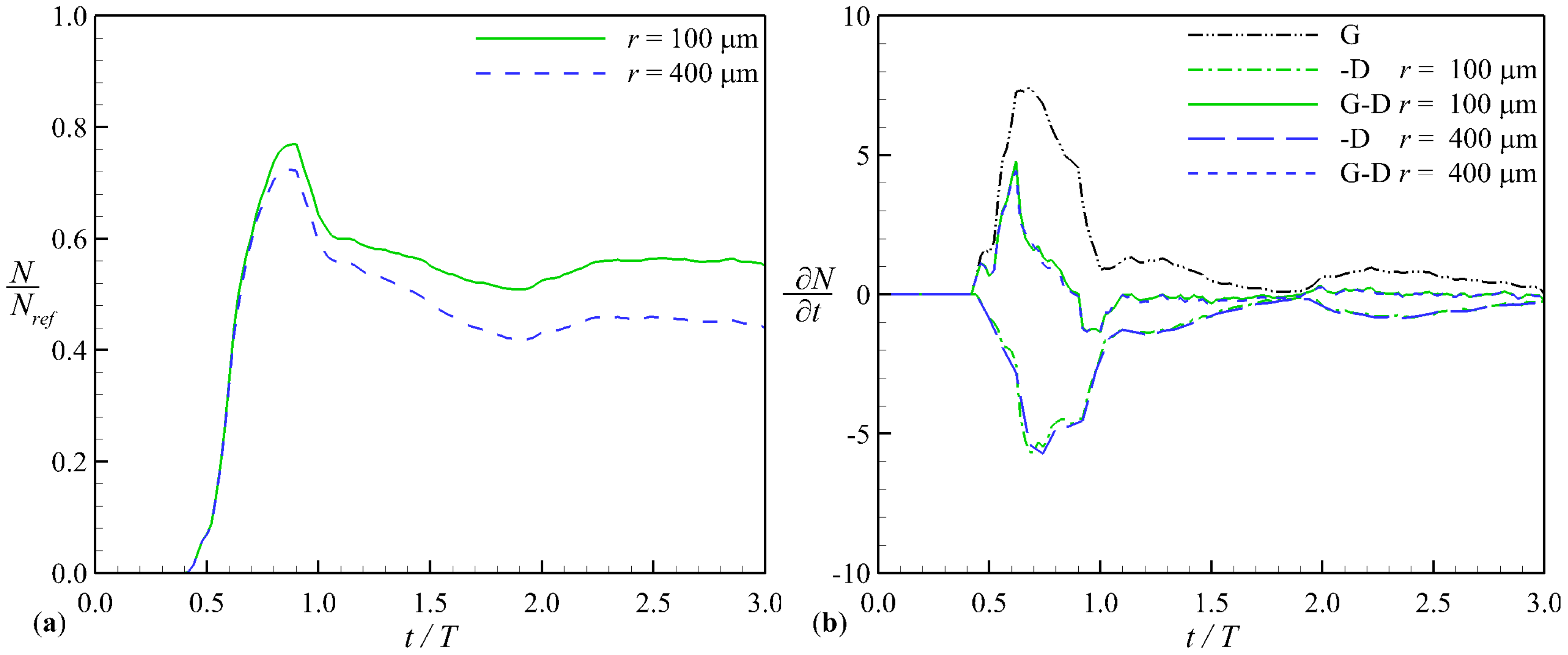
Figure 4a shows the time history of the total number of droplets in the air, N, in Case A55. The time rate of change of N is determined by the summation of the production rate G and disappearance rate as:
Here, G and D are defined as:
where and represent respectively the numbers of droplets generated at the wave surface and settling back to the water in a finite time duration from t to , and the limitation gives the instantaneous time rate of change of N due to the generation and disappearance. In the simulation, G and D at time step n are calculated as:
The histories of G, and in Case A55 are depicted in Figure 4b. As explained in Section 2.3, the effect of the droplet radius on the generation rate is not considered in the present simulations, so that the histories of G for droplets of µm and 400 µm are the same. Figure 4a shows that the value of N experiences a fast increase between and , when the first overturning jet is formed. After a short-term decrease, the value of N increases again between and during the second plunging event. The magnitude of for droplets of µm is larger than that of µm. As a result, the total number of droplets of µm is larger than that of µm. Note that the difference in N for droplets of different radii is caused by the time integration of the difference in . Although the values of for droplets of different radii are close to each other (Figure 4b), the difference of their time integrations can be more pronounced (Figure 4a).
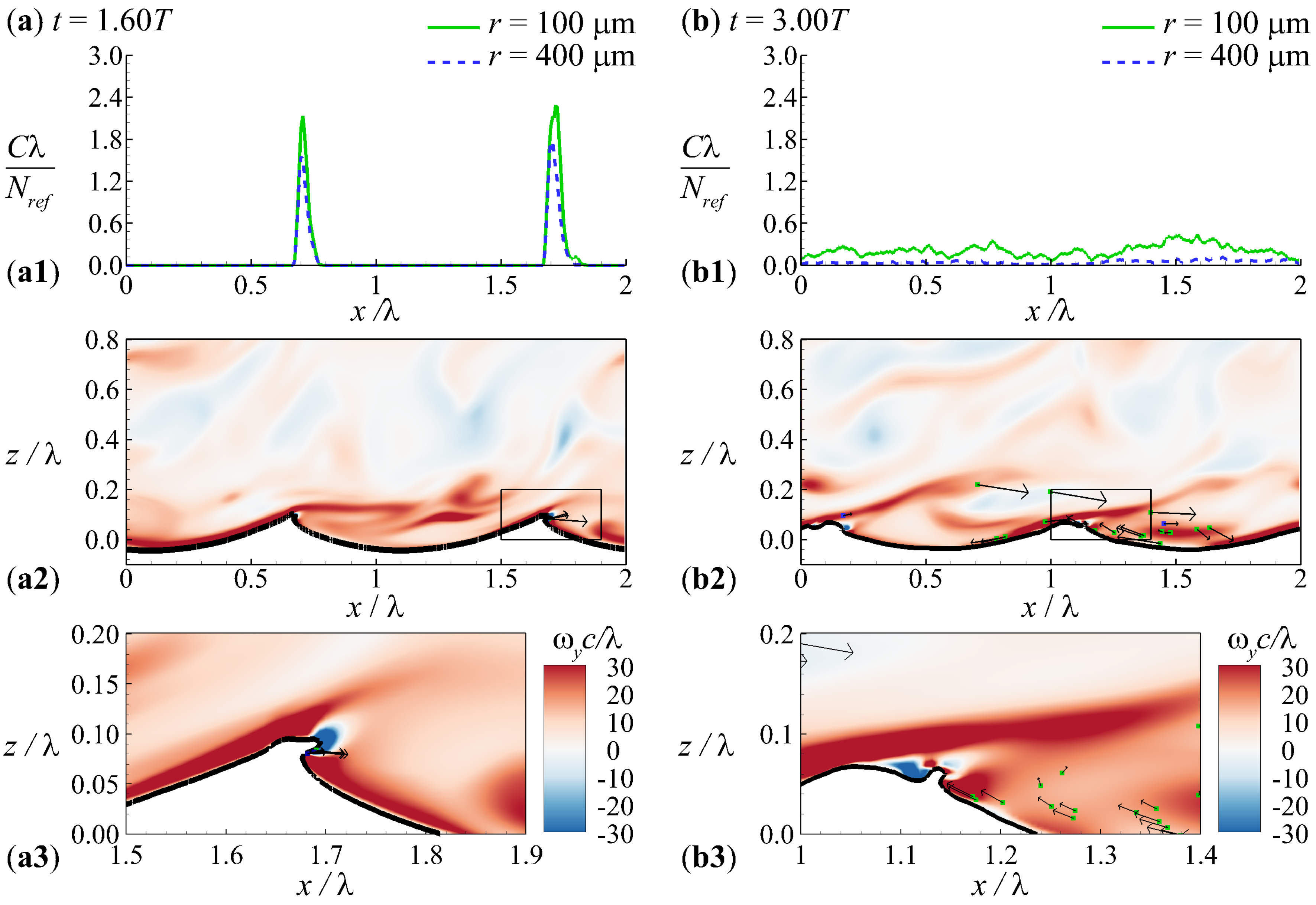
Next, we discuss the effects of wave steepness. Figure 5 shows the instantaneous distribution of droplets in Case A38, while Figure 6 demonstrates the time histories of the total number of droplets N, generation rate G and disappearance rate . The generation of droplets takes place later in Case A38 than in Case A55. Figure 6 shows that no droplet is generated before . The droplets are generated when a bulge is formed at the wave crest (Figure 5(a1)). The values of N and G increase at this stage. The number of droplets in Case A38 is much smaller than that in Case A55. Note that the vertical scale in Figure 6 is much smaller than that in Figure 4. A spanwise vortex is also found near the wave crest in Case A38. However, the size of the vortex in Case A38 is smaller than that in Case A55. Although the suspension effect of the vortex sends some droplets of µm to the altitude of at the late stage of wave breaking (Figure 5(b3)), most droplets fall back into water. As a result, the total number of droplets decreases after . The value of N for droplets of µm decreases faster than that of µm, consistent with the results in Case A55.
Thus far, we have shown the effects of wave steepness on the generation and transport of droplets by comparing Cases A55 and A38. Next, we further study the influences of the wave age through Cases B55 and C55. Figure 7 displays the distribution of droplets at different stages of wave breaking in Case B55, where the wave age is 12.0 as opposed to 3.7 in Case A55. From the comparisons between Figure 3a and Figure 7a and between Figure 3b and Figure 7b, it can be seen that the distribution of droplets in Case B55 is similar to that in Case A55 during the first plunging event. Large quantities of droplets are generated near the wave crest, when the overturning jet is formed (Figure 7a), and the upward-directed airflow in the downstream of the large-scale spanwise vortex suspends the droplets (Figure 7b). However, the second plunging event in Case B55 is not as violent as in Case A55, and as a result, less droplets are generated at this stage in Case B55. This is evident from the comparison between Figure 3(c1) and Figure 7(c1), which show that the horizontal profile of C forms a bimodal shape within each wave length in Case A55, while there is only one peak in each wave length in Case B55. At the late stage of wave breaking , the airflow separation is not shown in Case B55 (Figure 7d). The present observations of the airflow separation at different wave ages are consistent with the experimental results of Buckley and Veron [74], who found that airflow separation happens over young waves in their experiments, but not over more mature waves. Therefore, the spatial accumulation of droplets is absent at in Case B55. Due to the absence of the suspension effect caused by the airflow separation, the highest altitude that droplets reach in Case B55 is lower than that in Case A55, as evident from the comparison between Figure 3(f2) and Figure 7(d2).
Figure 8 shows the time histories of N, G and in Case B55. Different from Case A55, there is only one peak in the time histories of N and G in Case B55. As discussed above, the second peak is absent because the second plunging event in Case B55 is less violent. The values of for droplets of different radii are close to each other. As a result, the difference in the value of N between different droplet sizes in Case B55 is less significant than that in Case A55.
Figure 9 shows the distribution of droplets after the first plunging event in Case C55, for which the wave age is 27.7 (Table 1). The generation and transport of droplets during the first plunging event in Case C55 are similar to those in Cases A55 and B55. From Figure 10a, which shows the time history of N in Case C55, it is known that the total number of droplets also experiences a fast increase during the first plunging event. However, the value of N in Case C55 is smaller than that in Case A55, indicating that the high-speed wind in Case A55 (see Table 1) tends to enhance the generation of droplets, which is consistent with the observation in field measurements and laboratory experiments [12,16].
An interesting phenomenon in Case C55 is that from the comparison between Figure 3(e1) and Figure 9(a1), it can be seen that the number of droplets in the upstream of the wave crest is larger in Case C55 than in Case A55. This indicates that droplets are generated behind the wave crest in Case C55. Such a process of droplet generation over old waves has been observed by Veron [16] in laboratory experiments. The generation of droplets behind the wave crest lasts till , which in turn sustains the value of G at a high level (Figure 9b). As a result, the peak in the time history of N is wider in Case C55 than in Case A55.
The distribution of droplets at the late stage of wave breaking in Case C55 is similar to that in Case B55. Because there is no airflow separation in Cases B55 and C55, in these two cases, we observe no accumulation of droplets, in contrast to Case A55. It is known from the comparison among Figure 4a, Figure 8a and Figure 10a that after , the number of droplets of µm is significantly smaller in Cases B55 and C55 than in Case A55, due to the absence of airflow separation in Cases B55 and C55. In contrast, the numbers of droplets of µm in these three cases are close. As discussed above, this is because the airflow separation in Case A55 is not sufficiently strong to suspend large droplets.
Finally, we study the vertical distribution of the concentration of sea spray droplets , defined as:
where is the number of droplets in the interval between z and . In the simulation, the calculation of is simplified to:
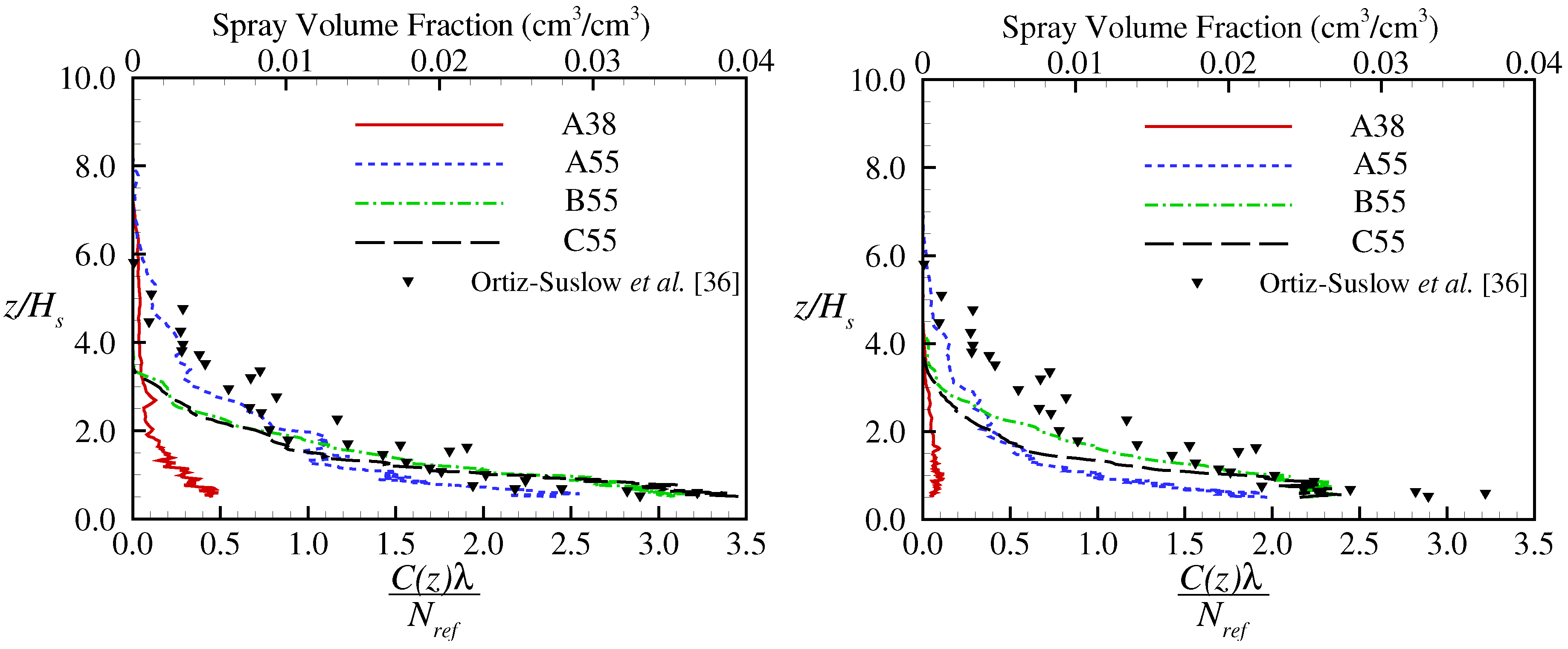
where is the grid size in the z-direction. Figure 11 compares the vertical profile of at the late stage of wave plunging () in all cases. The value of is normalized by , and the altitude z is normalized by the wave height . It is evident from Figure 11 that there are more droplets in Cases A55, B55 and C55 with plunging breakers than in Case A38 with spilling breakers. In the cases with plunging breakers, the concentration of droplets decreases as the altitude increases. The integral volume fraction of sea spray droplets of all scales at obtained from the laboratory experiment of Ortiz-Suslow et al. [36] is superposed in the figure for comparison. Note that the vertical profile of obtained from the simulation cannot be compared with the measurement results quantitatively, because the absolute value of the droplet number is unknown from the simulation. The lower horizontal axis gives the scale of of our simulation, and the upper horizontal axis gives the scale of the integral spray volume fraction of Ortiz-Suslow et al. [36]. However, the shape of the profile of in Case A55 is in agreement with that of the integral spray volume fraction obtained from the laboratory experiments of Ortiz-Suslow et al. [36]. Furthermore, both numerical and experimental results show that the sea spray droplets reach a high altitude at . In contrast, the droplets reach a lower altitude in Cases B55 and C55 with medium and old waves. As shown in Figure 11, sea spray droplets of both µm and µm only reach approximately.
4. Discussion
While the results demonstrated in this paper indicate that fine-scale high-resolution numerical simulations can serve as a useful tool for studying the generation and transport of sea spray droplets, the present simulations are only the first step towards the computation and prediction of the sea spray droplets in the complex wind and wave system. There are some limitations in the present study. For example, the results analysis in the present simulation is limited by the unsteadiness of wave breaking. We cannot perform time-averaging as has been done in many studies for other types of flows with simpler configurations [38,39,40,77] to define turbulence statistics. In the future, it is important to perform multiple runs with the same wave geometry and wind profile, but different instantaneous turbulence fluctuations to define turbulence statistics based on the ensemble-averaging over different runs. Furthermore, due to the lack of the detailed information on the sea spray generation function (SSGF) at the air–water interface, the effect of wind speed and droplet radius on the generation rate of sea spray cannot be addressed in the present simulations, and as a consequence, direct comparison of the present numerical results with the measurement results cannot be conducted. It is unrealistic to expect that numerical simulation can resolve everything, and it is more appropriate to rely on measurement data. The radius spectra of droplets measured in experiments will be needed to determine the numbers of droplets generated at different radii, and the measurement of the droplet ejection velocity will also be valuable. Furthermore, the feedback of droplets to the airflow is not considered in the present study. The Reynolds number and wind speed of practical interest also need to be considered in the future. Although the wind speeds in Cases A35 and A55 are close to a hurricane wind speed, the Reynolds number is not realistic because of the use of the artificial viscosity. LES with the proper wall-layer model near the wave surface needs to be developed to conduct simulations with parameters of practical interest. The encouraging results shown in this paper indicate that the computational framework established in this study can serve as a useful tool to investigate these effects and to incorporate measurement data from advanced experiments in the future.
5. Conclusions
In this study, a DNS method has been developed to study the generation and transport of spume droplets in wind over breaking waves, with the wave breaking process resolved explicitly. In the simulation, the air and water are treated as a coupled system, with the interface captured using the CLSVOF method. The trajectories of droplets are tracked using the LPT method. Droplets of two different radii are considered. The effects of wave age and wave steepness are analyzed through four simulation cases.
Plunging breakers generate a large amount of droplets. At young and intermediate wave ages, droplets are generated at the wave crest, but at the old wave age, droplets are also generated behind the wave crest with respect to the wave-propagation direction. The large-scale spanwise vortex induced in the plunging event plays an important role in suspending the droplets. There are two violent plunging events in the young wave case, and consequently, two peaks occur in the time history of the number of droplets. In the intermediate and old wave age cases, there is only one peak in the time history of the total number of droplets, because the second plunging event is much milder. Large droplets are more difficult to suspend, such that the disappearance rate of large droplets is higher than that of small droplets. At the late stage of wave breaking, the airflow separation over the wave crest causes small droplets to accumulate along the shear layer. Over intermediate and old waves, compared with the young wave case, airflow separation is not present, and no spatial accumulation of droplets is observed at the late stage of wave breaking. Different from the plunging breakers, spilling breakers generate much less droplets. Because no large-scale spanwise vortex occurs in the spilling event, the process of droplet suspension is absent during spilling wave breaking. As a result, the number of droplets in air over spilling breakers is much smaller than that over plunging breakers.
Supplementary Materials
The following are available online at www.mdpi.com/2073-4433/8/12/248/s1, Video S1: Spume droplets’ motion in Case A55.
Acknowledgments
Shuai Tang and Yu-Hong Dong would like to thank the Natural Science Foundation of China for its support (Award number 11572183) to this research. Shuai Tang also acknowledges the China Scholarship Council for sponsoring his visit to the University of Minnesota from June 2015 to June 2017. Zixuan Yang and Lian Shen would like to thank the support from ONR (Award number N00014-16-1-3205) and MN Sea Grant (Grant number R/CC-09-16).
Author Contributions
Yu-Hong Dong and Lian Shen conceived of and designed the numerical simulations. Shuai Tang, Zixuan Yang and Caixi Liu contributed simulation tools. Shuai Tang performed the numerical simulations. Shuai Tang and Zixuan Yang analyzed the data. Shuai Tang, Zixuan Yang, Yu-Hong Dong and Lian Shen wrote the paper.
Conflicts of Interest
The authors declare no conflict of interest.
Abbreviations
The following abbreviations are used in this manuscript:
| MABL | Marine atmosphere boundary layer |
| LPT | Lagrangian particle tracking |
| DNS | Direct numerical simulation |
| LS | Level-set |
| VOF | Volume of fluid |
| CLSVOF | Coupled level-set and volume-of-fluid |
| LES | Large eddy simulation |
| SSGF | Sea spray generation function |
References
- Andreas, E.L. Spray stress revisited. J. Phys. Oceanogr. 2004, 34, 1429–1440. [Google Scholar] [CrossRef]
- Mueller, J.A.; Veron, F. Impact of sea spray on air-sea fluxes. Part II: Feedback effects. J. Phys. Oceanogr. 2014, 44, 2835–2853. [Google Scholar] [CrossRef]
- Iida, N.; Toba, Y. Effect of sea-water droplets on evaporation from sea surface. In The Wind-Driven Air-Sea Interface; Banner, M., Ed.; School of Mathematics, University of South Wales: Sydney, Australia, 1999; pp. 325–332. [Google Scholar]
- Edson, J.; Paluszkiewicz, T.; Sandgathe, S.; Vincent, L.; Goodman, L.; Curtin, T.; Hollister, J.; Colton, M. Coupled Marine Boundary Layers and Air-Sea Interaction Initiative: Combining Process Studies, Simulations, and Numerical Models (Revision 5.0); Office of Naval Research: Arlington, TX, USA, 1999; pp. 41–45. [Google Scholar]
- Spiel, D.E. On the birth of film drops from bubbles on seawater surface. J. Geophys. Res. Oceans 1998, 103, 24907–24918. [Google Scholar] [CrossRef]
- O’Dowd, C.D.; de Leeuw, G. Marine aerosol production; A review of the current knowledge. Philos. Trans. R. Soc. Lond. Ser. A 2007, 365, 1753–1774. [Google Scholar] [CrossRef] [PubMed]
- Fuentes, E.; Coe, H.; Green, D.; de Leeuw, G.; McFiggans, G. Laboratory-generated primary marine aerosol via bubble-bursting and atomization. Atmos. Meas. Tech. 2010, 3, 141–162. [Google Scholar] [CrossRef]
- Monahan, E.C.; Spiel, D.E.; Davidson, K.L. A model of marine aerosol generation via whitecaps and wave disruption. In Oceanic Whitecaps; Springer: Dordrecht, The Netherlands, 1986; pp. 167–174. [Google Scholar]
- Kientzler, C.F.; Arons, A.B.; Blanchard, D.C.; Woodcock, A.H. Photographic investigation of the projection of droplets by bubbles bursting at a water surface. Tellus 1954, 6, 1–7. [Google Scholar] [CrossRef]
- MacIntyre, F. Flow patterns in breaking bubbles. J. Geophys. Res. 1972, 77, 5211–5228. [Google Scholar] [CrossRef]
- Spiel, D.E. More on the births of jet drops from bubbles bursting on seawater surfaces. J. Geophys. Res. Oceans 1997, 102, 5815–5821. [Google Scholar] [CrossRef]
- Andreas, E.L. A review of the sea spray generation function for the open ocean. In Atmosphere-Ocean Interactions; Perrie, W.A., Ed.; WIT Press: Southampton, UK, 2002; pp. 1–46. [Google Scholar]
- Wu, J. Production of spume drops by the wind tearing of wave crests: The search for quantification. J. Geophys. Res. Oceans 1993, 98, 18221–18227. [Google Scholar] [CrossRef]
- Andreas, E.L.; Edson, J.; Monahan, E.B.; Rouault, M.C.; Smith, S.D. The spray contribution to net evaporation from the sea: A review of recent progress. Bound.-Layer Meteorol. 1995, 72, 3–52. [Google Scholar] [CrossRef]
- Marmottant, P.; Villermaux, E. On spray formation. J. Fluid Mech. 2004, 498, 73–111. [Google Scholar] [CrossRef]
- Veron, F. Ocean Spray. Annu. Rev. Fluid Mech. 2015, 47, 507–538. [Google Scholar] [CrossRef]
- Preobrazhenskii, L. Estimate of the content of spray drops in the near-water layer of the atmosphere. Fluid Mech. Sov. Res. 1973, 2, 95–100. [Google Scholar]
- Koga, M. Direct production of droplets from breaking wind-wave—Its observation by a multi-colored overlapping exposure photographing technique. Tellus 1981, 33, 552–563. [Google Scholar] [CrossRef]
- Andreas, E.L. Sea spray and the turbulent air-sea heat fluxes. J. Geophys. Res. Oceans 1992, 97, 11429–11441. [Google Scholar] [CrossRef]
- Andreas, E.L. A new sea spray generation function for wind speeds up to 32 ms−1. J. Phys. Oceanogr. 1998, 28, 2175–2184. [Google Scholar] [CrossRef]
- Fairall, C.W.; Kepert, J.D.; Holland, G.J. The effect of sea spray on surface energy transports over the ocean. Glob. Atmos. Ocean Syst. 1994, 2, 121–142. [Google Scholar]
- Veron, F.; Hopkins, C.; Harrison, E.L.; Muelluer, J.A. Sea spray spume droplet production in high wind speeds. Geophys. Res. Lett. 2012, 39, L16602. [Google Scholar] [CrossRef]
- Smith, M.H.; Park, P.M.; Consterdine, I.E. Marine aerosol concentrations and estimated fluxes over the sea. Q. J. R. Meteorol. Soc. 1993, 119, 809–824. [Google Scholar] [CrossRef]
- Zhao, D.; Toba, Y.; Sugioka, K.I.; Komori, S. New sea spray generation function for spume droplets. J. Geophys. Res. Oceans 2006, 111. [Google Scholar] [CrossRef]
- Mueller, J.A.; Veron, F. A sea state dependent spume generation function. J. Phys. Oceanogr. 2009, 39, 2363–2372. [Google Scholar] [CrossRef]
- Shi, J.; Zhao, D.; Li, X.; Zhong, Z. New wave-dependent formulae for sea spray flux at air-sea interface. J. Hydrodyn. Ser. B 2009, 21, 573–581. [Google Scholar] [CrossRef]
- Kudryavtsev, V.N. On the effect of sea drops on the atmospheric boundary layer. J. Geophys. Res. Oceans 2006, 111. [Google Scholar] [CrossRef]
- Ovadnevaite, J.; de Leeuw, G.; Ceburnis, D.; Monahan, C.; Partanen, A.I.; Korhonen, H.; O’Dowd, C.D. A sea spray aerosol flux parameterization encapsulating wave state. Atmos. Chem. Phys. 2014, 14, 1837–1852. [Google Scholar] [CrossRef] [Green Version]
- Kudryavtsev, V.N.; Makin, V.K. Impact of ocean spray on the dynamic of the marine atmospheric boundary layer. Bound.-Layer Meteorol. 2011, 140, 383–410. [Google Scholar] [CrossRef]
- Rastigejev, Y.; Suslov, S.A.; Lin, Y.L. Effect of ocean spray on vertical momentum transport under high-wind conditions. Bound.-Layer Meteorol. 2011, 141, 1–20. [Google Scholar] [CrossRef]
- Rastigejev, Y.; Suslov, S.A. E-ϵ model of spray-laden near-sea atmospheric layer in high wind conditions. J. Phys. Oceanogr. 2014, 44, 742–763. [Google Scholar] [CrossRef]
- Wu, L.; Rutgersson, A.; Sahlée, E.; Larsén, X.G. The impact of waves and sea spray on modelling storm track and development. Tellus A Dyn. Meteorol. Oceanogr. 2015, 67, 27967. [Google Scholar] [CrossRef] [Green Version]
- Zhang, T.; Song, J.; Li, S.; Yang, L. The effects of wind-driven waves and ocean spray on the drag coefficient and near-surface wind profiles over the ocean. Acta Oceanol. Sin. 2016, 35, 79–85. [Google Scholar] [CrossRef]
- Rastigejev, Y.; Suslov, S.A. Two-temperature nonequilibrium model of a marine boundary layer laden with evaporating ocean spray under high-wind conditions. J. Phys. Oceanogr. 2016, 46, 3083–3102. [Google Scholar] [CrossRef]
- Ortiz-Suslow, D.G.; Haus, B.K.; Mehta, S.; Laxague, N.J. A laboratory study of spray generation in high winds. In IOP Conference Series: Earth and Environmental Science; IOP Publishing: Bristol, UK, 2016; Volume 35. [Google Scholar]
- Ortiz-Suslow, D.G.; Haus, B.K.; Mehta, S.; Laxague, N.J. Sea spray generation in very high winds. J. Atmos. Sci. 2016, 73, 3975–3995. [Google Scholar] [CrossRef]
- Troitskaya, Y.; Kandaurov, A.; Ermakova, O.; Kozlov, D.; Sergeev, D.; Zilitinkevich, S. Bag-breakup fragmentation as the dominant mechanism of sea-spray production in high winds. Sci. Rep. 2017, 7, 1614. [Google Scholar] [CrossRef] [PubMed]
- Richter, D.H.; Sullivan, P.P. Sea surface drag and the role of spray. Geophys. Res. Lett. 2013, 40, 656–660. [Google Scholar] [CrossRef]
- Richter, D.H.; Sullivan, P.P. Momentum transfer in a turbulent, particle-laden Couette flow. Phys. Fluids 2013, 25, 053304. [Google Scholar] [CrossRef]
- Richter, D.H.; Sullivan, P.P. The sea spray contribution to sensible heat flux. J. Atmos. Sci. 2014, 71, 640–654. [Google Scholar] [CrossRef]
- Druzhinin, O.A.; Troitskaya, Y.I.; Zilitinkevich, S.S. The study of droplet-laden turbulent airflow over waved water surface by direct numerical simulation. J. Geophys. Res. Oceans 2017, 122, 1789–1807. [Google Scholar] [CrossRef]
- Banner, M.L.; Peregrine, D.H. Wave breaking in deep water. Annu. Rev. Fluid Mech. 1993, 25, 373–397. [Google Scholar] [CrossRef]
- Sullivan, P.P.; McWilliams, J.C. Dynamics of winds and currents coupled to surface waves. Annu. Rev. Fluid Mech. 2010, 42, 19–42. [Google Scholar] [CrossRef]
- Perlin, M.; Choi, W.; Tian, Z. Breaking waves in deep and intermediate waters. Annu. Rev. Fluid Mech. 2013, 45, 115–145. [Google Scholar] [CrossRef]
- Lamb, K.G. Internal wave breaking and dissipation mechanisms on the continental slope/shelf. Annu. Rev. Fluid Mech. 2014, 46, 231–254. [Google Scholar] [CrossRef]
- Harlow, F.H.; Welch, J.E. Numerical calculation of time-dependent viscous incompressible flow of fluid with free surface. Phys. Fluids 1965, 8, 2182–2189. [Google Scholar] [CrossRef]
- Miyata, H.; Nishimura, S.; Masuko, A. Finite difference simulation of nonlinear waves generated by ships of arbitrary three-dimensional configuration. J. Comput. Phys. 1985, 60, 391–436. [Google Scholar] [CrossRef]
- Miyata, H. Finite-difference simulation of breaking waves. J. Comput. Phys. 1986, 65, 179–214. [Google Scholar] [CrossRef]
- Osher, S.; Sethian, J.A. Fronts propagating with curvature-dependent speed: Algorithms based on Hamilton-Jacobi formulations. J. Comput. Phys. 1988, 79, 12–49. [Google Scholar] [CrossRef]
- Sussman, M.; Smereka, P.; Osher, S. A level set approach for computing solutions to incompressible two-phase flow. J. Comput. Phys. 1994, 114, 146–159. [Google Scholar] [CrossRef]
- Zhang, Y.; Zou, Q.; Greaves, D. Numerical simulation of free-surface flow using the level-set method with global mass correction. Int. J. Numer. Methods Fluids 2010, 63, 651–680. [Google Scholar] [CrossRef]
- Scardovelli, R.; Zaleski, S. Direct numerical simulation of free-surface and interfacial flow. Annu. Rev. Fluid Mech. 1999, 31, 567–603. [Google Scholar] [CrossRef]
- Lopez, J.; Hernandez, J.; Gomez, P.; Faura, F. An improved PLIC-VOF method for tracking thin fluid structures in incompressible two-phase flows. J. Comput. Phys. 2005, 208, 51–74. [Google Scholar] [CrossRef]
- Weymouth, G.D.; Yue, D.K. Conservative volume-of-fluid method for free-surface simulations on Cartesian-grids. J. Comput. Phys. 2010, 229, 2853–2865. [Google Scholar] [CrossRef]
- Sussman, M.; Puckett, E.G. A coupled level set and volume-of-fluid method for computing 3D and axisymmetric incompressible two-phase flows. J. Comput. Phy. 2000, 162, 301–337. [Google Scholar] [CrossRef]
- Lv, X.; Zou, Q.; Zhao, Y.; Reeve, D. A novel coupled level set and volume of fluid method for sharp interface capturing on 3D tetrahedral grids. J. Comput. Phys. 2010, 229, 2573–2604. [Google Scholar] [CrossRef]
- Liu, Y. Numerical Study of Strong Free Surface Flow and Breaking Waves. Ph.D Thesis, The Johns Hopkins University, Baltimore, MD, USA, 2012. [Google Scholar]
- Chen, G.; Kharif, C.; Zaleski, S.; Li, J. Two-dimensional Navier-Stokes simulation of wave breaking. Phys. Fluids 1999, 11, 121–133. [Google Scholar] [CrossRef] [Green Version]
- Song, C.; Sirviente, A.I. A numerical study of breaking waves. Phys. Fluids 2004, 16, 2649–2667. [Google Scholar] [CrossRef]
- Iafrati, A. Numerical study of the effects of the breaking intensity on wave breaking flows. J. Fluid Mech. 2009, 622, 371–411. [Google Scholar] [CrossRef]
- Hu, Y.; Guo, X.; Lu, X.; Liu, Y.; Dalrymple, R.A.; Shen, L. Idealized numerical simulation of breaking water wave propagating over a viscous mud layer. Phys. Fluids 2012, 24, 112104. [Google Scholar] [CrossRef]
- Deike, L.; Popinet, S.; Melville, W.K. Capillary effects on wave breaking. J. Fluid Mech. 2015, 769, 541–569. [Google Scholar] [CrossRef]
- Lubin, P.; Glockner, S. Numerical simulations of three-dimensional plunging breaking waves: Generation and evolution of aerated vortex filaments. J. Fluid Mech. 2015, 767, 364–393. [Google Scholar] [CrossRef]
- Deike, L.; Melville, W.K.; Popinet, S. Air entrainment and bubble statistics in breaking waves. J. Fluid Mech. 2016, 801, 91–129. [Google Scholar] [CrossRef]
- Kim, J.; Moin, P. Application of a fractional-step method to incompressible Navier-Stokes equations. J. Comput. Phys. 1985, 59, 308–323. [Google Scholar] [CrossRef]
- Balay, S.; Brown, K.; Eijkhout, V.; Gropp, W.; Kaushik, D.; Knepley, M.; Mcinnes, L.C.; Smith, B.; Zhang, H. PETSc Users Manual; Revision 3.3; Computer Science Division, Argonne National Laboratory: Argonne, IL, USA, 2012.
- Yang, Z.; Lu, X.-H.; Guo, X.; Liu, Y.; Shen, L. Numerical simulation of sediment suspension and transport under plunging breaking waves. Comput. Fluids 2017, 158, 57–71. [Google Scholar] [CrossRef]
- McLaughlin, J.B. Aerosol particle deposition in numerically simulated channel flow. Phys. Fluids 1989, 1, 1211–1224. [Google Scholar] [CrossRef]
- Dong, Y.-H.; Chen, L.-F. The effect of stable stratification and thermophoresis on fine particle deposition in a bounded turbulent flow. Int. J. Heat Mass Transf. 2011, 54, 1168–1178. [Google Scholar] [CrossRef]
- Zhao, L.H.; Anderson, H.I.; Gillissen, J. Turbulence modulation and drag reduction by spherical particles. Phys. Fluids 2010, 22, 081702. [Google Scholar] [CrossRef]
- Maxey, M.R.; Riley, J.J. Equation of motion for a small rigid sphere in a nonuniform flow. Phys. Fluids 1983, 26, 883–889. [Google Scholar] [CrossRef]
- Clift, R.; Grace, J.R.; Weber, M.E. Bubbles, Drops and Particles; Academic Press: Cambridge, MA, USA, 1978. [Google Scholar]
- Elghobashi, S.; Truesdell, G.C. Direct simulation of particle dispersion in a decaying isotropic turbulence. J. Fluid Mech. 1992, 242, 655–700. [Google Scholar] [CrossRef]
- Buckley, M.P.; Veron, F. Structure of the airflow above surface waves. J. Phys. Oceanogr. 2016, 46, 1377–1397. [Google Scholar] [CrossRef]
- Moin, P.; Mahesh, K. Direct numerical simulation: A tool in turbulence research. Annu. Rev. Fluid Mech. 1998, 30, 539–578. [Google Scholar] [CrossRef]
- Ninto, Y.; Garcia, M.H. Experiments on particle turbulence interactions in the near wall region of an open channel flow: Implications for sediment transport. J. Fluid Mech. 1996, 326, 285–319. [Google Scholar] [CrossRef]
- Liu, C.; Tang, S.; Shen, L.; Dong, Y. Characteristics of turbulence transport for momentum and heat in particle-laden turbulent vertical channel flows. Acta Mech. Sin. 2017, 33, 833–845. [Google Scholar] [CrossRef]
Figure 1.
Computational domain and coordinate system in the simulations.

Figure 2.
Successive snapshots of the three-dimensional field of droplets at (a) t = 0.4T, (b) t = 0.5T, (c) t = 1.0T, and (d) t = 3.0T in Case A55.
Figure 2.
Successive snapshots of the three-dimensional field of droplets at (a) t = 0.4T, (b) t = 0.5T, (c) t = 1.0T, and (d) t = 3.0T in Case A55.
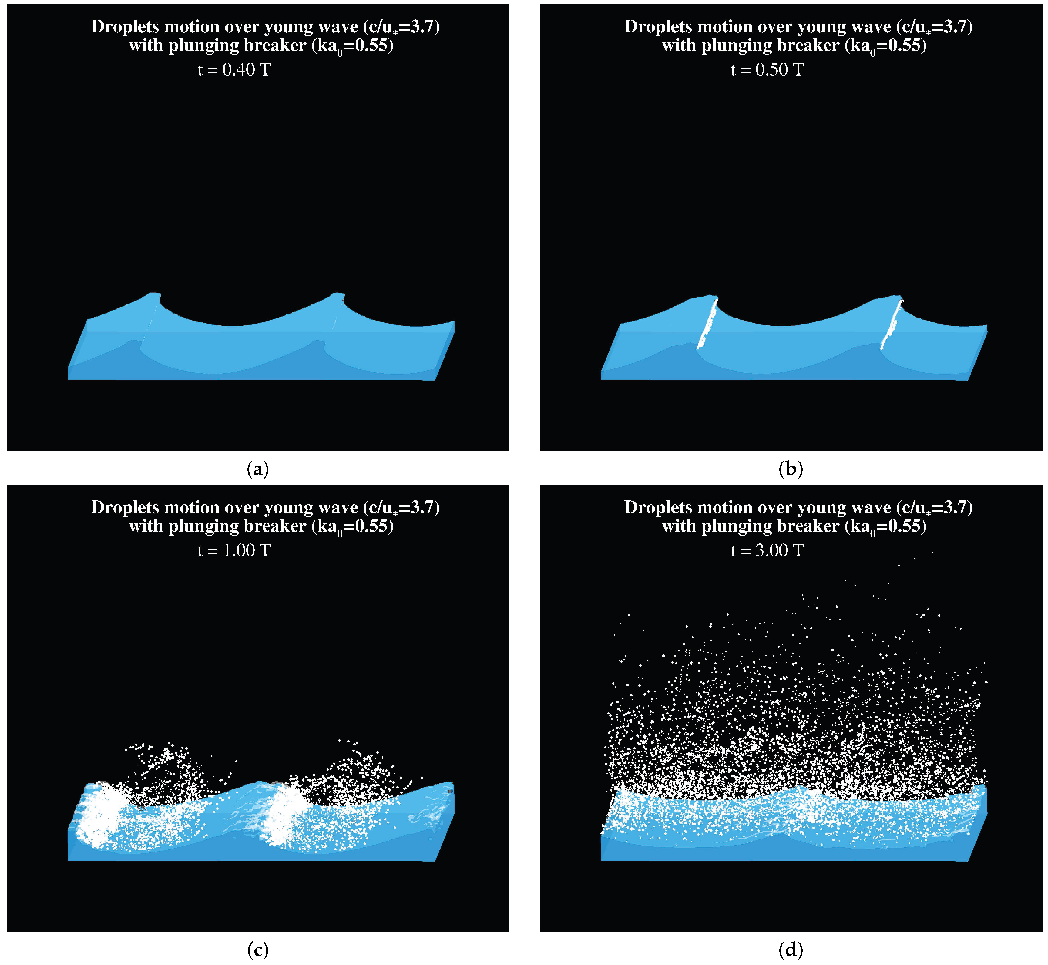
Figure 3.
Instantaneous distribution of droplets in Case A55 at (a) t = 0.54T, (b) t = 0.70T, (c) t = 0.90T, (d) t = 1.04T, (e) t = 1.20T, and (f) t = 3.00T. The upper panels of each figure show the streamwise profile of the droplet concentration . The middle panels show the projected positions of droplets in a spanwise plane. Green and blue dots denote droplets of µm and 400 µm, respectively. Only of the droplets are shown in the figure for clearer visualization. The vectors represent the in-plane relative velocity with respect to the wave phase speed c. Contours of the instantaneous spanwise vorticity of the airflow in the plane are superimposed. The thick solid lines represent the instantaneous air–water interface in the same plane. The lower panels show the zoom-in view of the region denoted by the box in the middle panel, and only of the droplets are demonstrated for clearer visualization. The wave propagates in the -direction.
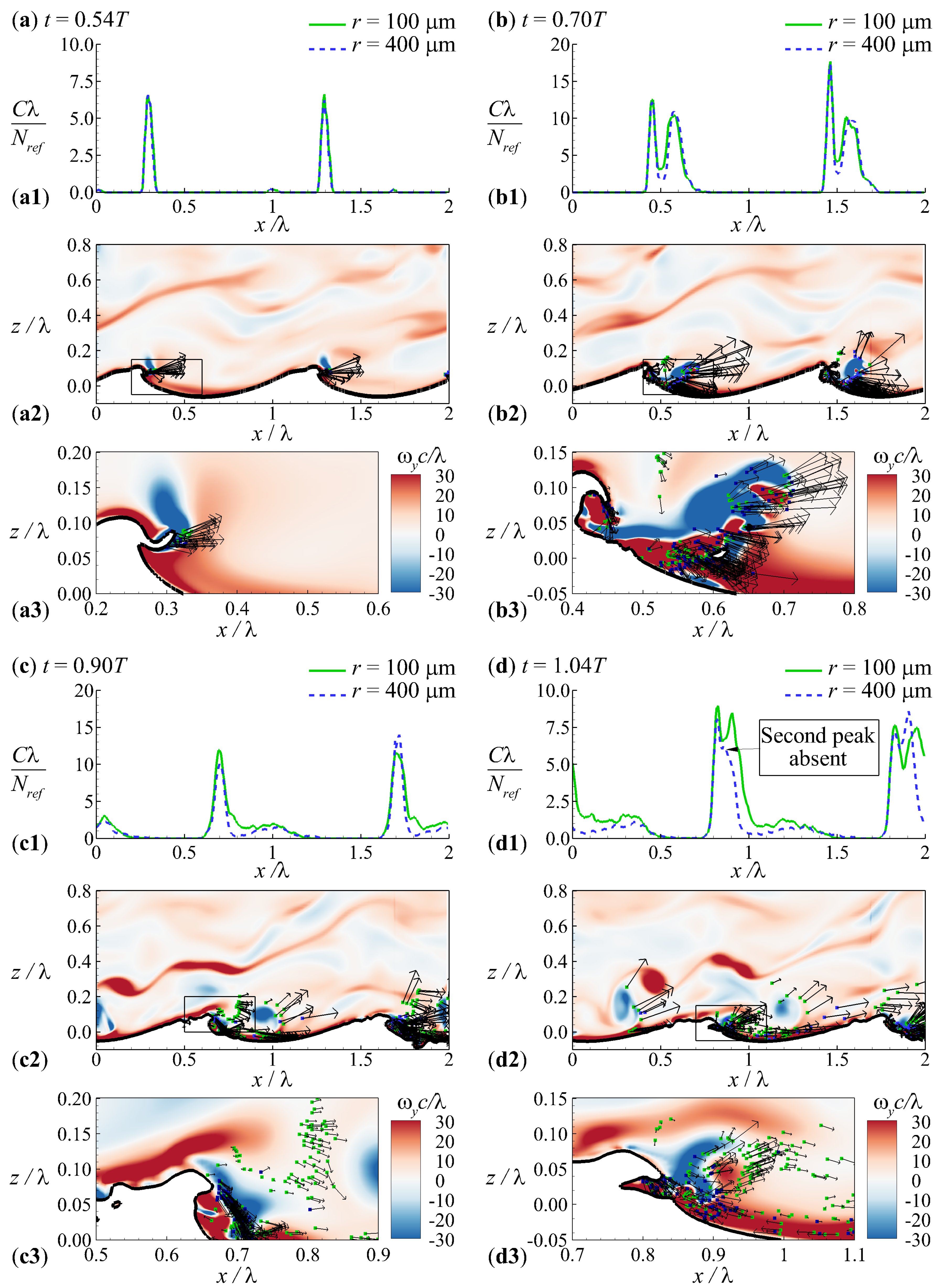

Figure 4.
Time histories of (a) the number of droplets , and (b) generation rate and disappearance rate of droplets in Case A55.
Figure 4.
Time histories of (a) the number of droplets , and (b) generation rate and disappearance rate of droplets in Case A55.
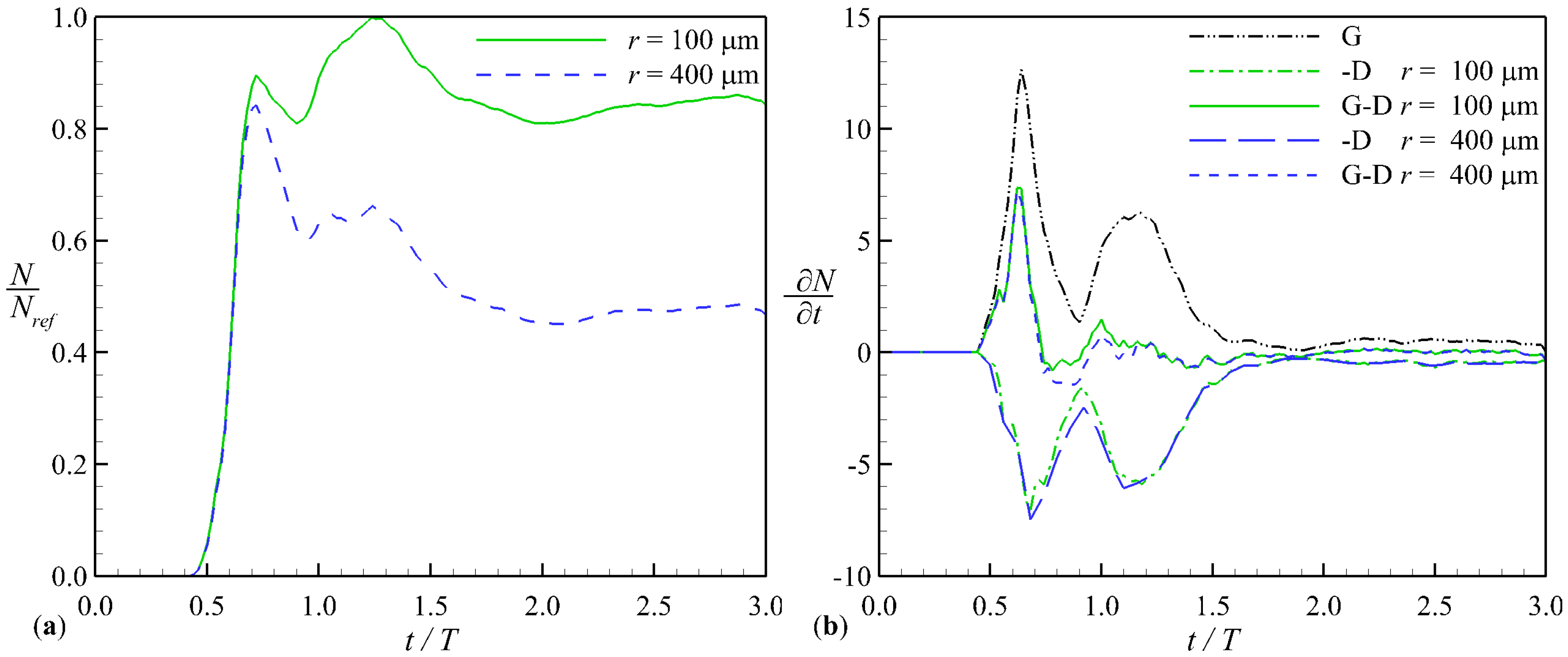
Figure 5.
See Figure 3 for the caption. Here, the results of Case A38 at (a) t = 1.60T and (b) t = 3.00T are shown instead.
Figure 5.
See Figure 3 for the caption. Here, the results of Case A38 at (a) t = 1.60T and (b) t = 3.00T are shown instead.

Figure 6.
Time histories of (a) the number of droplets , and (b) generation rate and disappearance rate of droplets in Case A38.
Figure 6.
Time histories of (a) the number of droplets , and (b) generation rate and disappearance rate of droplets in Case A38.
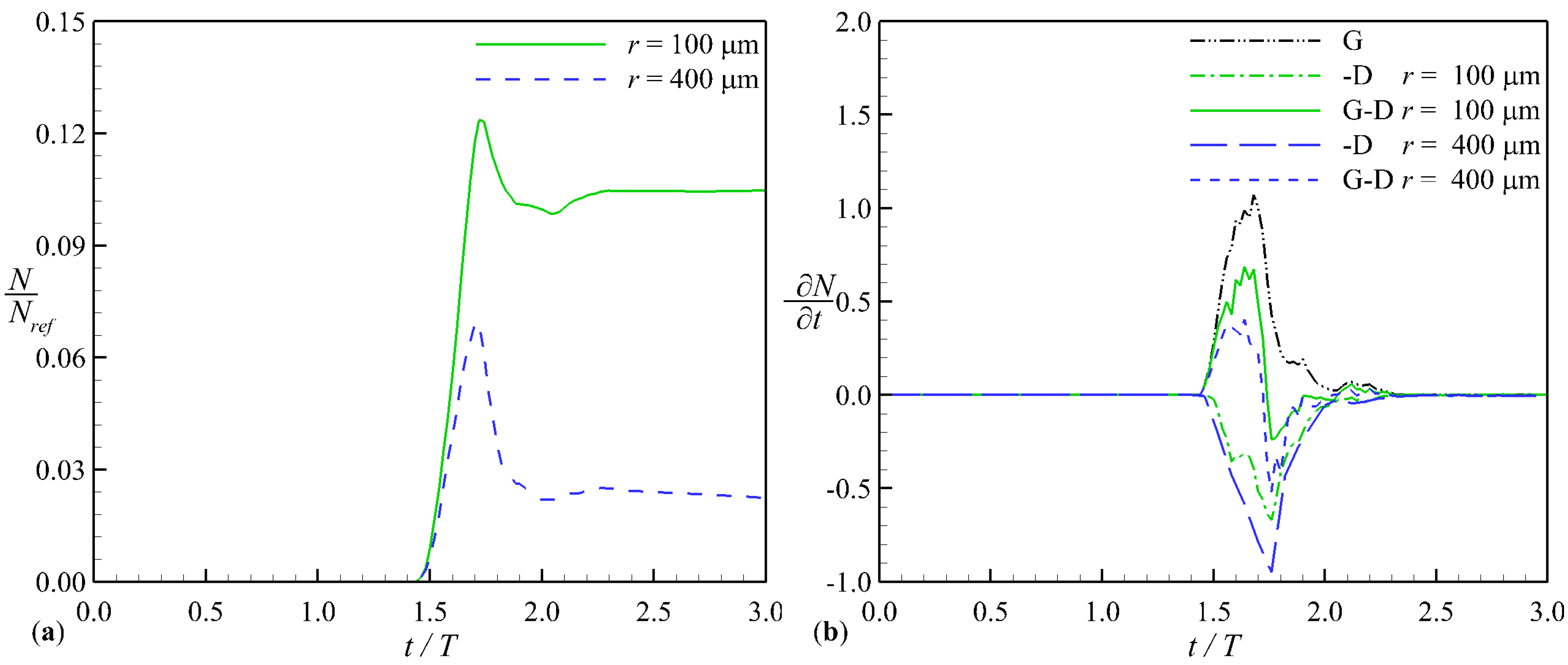
Figure 7.
See Figure 3 for the caption. Here, the results of Case B55 at (a) t = 0.54T, (b) t = 0.70T, (c) t = 1.20T, and (d) t = 3.00T are shown instead.
Figure 7.
See Figure 3 for the caption. Here, the results of Case B55 at (a) t = 0.54T, (b) t = 0.70T, (c) t = 1.20T, and (d) t = 3.00T are shown instead.


Figure 8.
Time histories of (a) the number of droplets , and (b) generation rate and disappearance rate of droplets in Case B55.
Figure 8.
Time histories of (a) the number of droplets , and (b) generation rate and disappearance rate of droplets in Case B55.

Figure 9.
See Figure 3 for the caption. Here, the results of Case C55 at (a) t = 1.20T and (b) t = 3.00T are shown instead.
Figure 9.
See Figure 3 for the caption. Here, the results of Case C55 at (a) t = 1.20T and (b) t = 3.00T are shown instead.

Figure 10.
Time histories of (a) the number of droplets , and (b) generation rate and disappearance rate of droplets in Case C55.
Figure 10.
Time histories of (a) the number of droplets , and (b) generation rate and disappearance rate of droplets in Case C55.
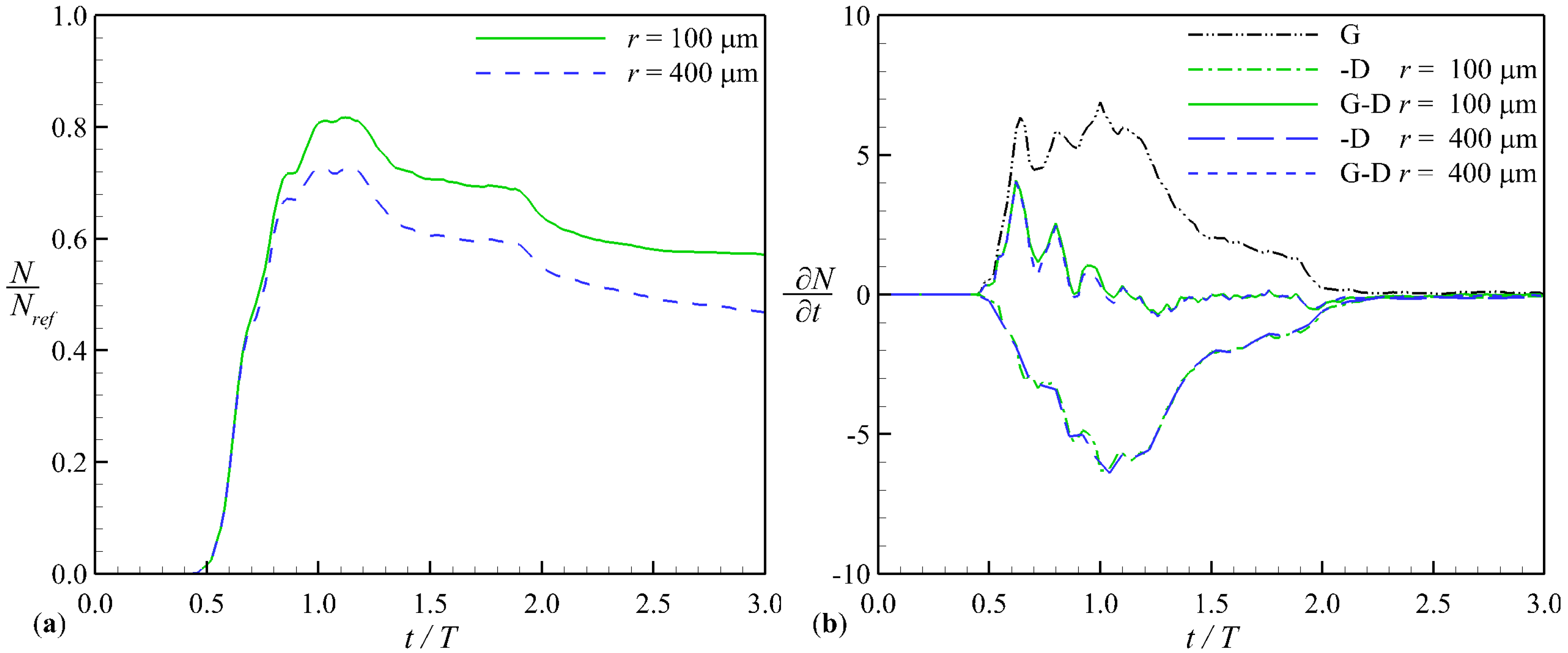
Figure 11.
Instantaneous vertical profile of the concentration of sea spray droplets of (a) µm and (b) µm at the late stage of wave plunging (). The integral volume fraction of sea spray droplets of all scales at obtained from the laboratory experiment of Ortiz-Suslow et al. [36] is superposed in the figure for comparison. The lower horizontal axis gives the scale of of our simulation. The upper horizontal axis gives the scale of the integral spray volume fraction of Ortiz-Suslow et al. [36].

Table 1.
Computational parameters for the simulation cases considered in this study.
| Dimensional Parameters | ||||||
| Case | ||||||
| A55 | 5 | 0.88 | 3.19 | 0.86 | 25.8 | 1.57 |
| A38 | 0.60 | 2.99 | 0.81 | 24.1 | 1.68 | |
| B55 | 0.88 | 3.19 | 0.27 | 8.1 | 1.57 | |
| C55 | 0.88 | 3.19 | 0.12 | 3.4 | 1.57 | |
| Dimensional Parameters | ||||||
| Case | ||||||
| A55 | 1.205 | 998 | 1.87 | |||
| A38 | 1.76 | |||||
| B55 | 0.59 | |||||
| C55 | 0.26 | |||||
| Dimensionless Parameters | ||||||
| Case | ||||||
| A55 | 3.7 | 0.55 | 180 | |||
| A38 | 3.7 | 0.38 | ||||
| B55 | 12.0 | 0.55 | ||||
| C55 | 27.7 | 0.55 | ||||
© 2017 by the authors. Licensee MDPI, Basel, Switzerland. This article is an open access article distributed under the terms and conditions of the Creative Commons Attribution (CC BY) license (http://creativecommons.org/licenses/by/4.0/).
Share and Cite
MDPI and ACS Style
Tang, S.; Yang, Z.; Liu, C.; Dong, Y.-H.; Shen, L. Numerical Study on the Generation and Transport of Spume Droplets in Wind over Breaking Waves. Atmosphere 2017, 8, 248. https://doi.org/10.3390/atmos8120248
AMA Style
Tang S, Yang Z, Liu C, Dong Y-H, Shen L. Numerical Study on the Generation and Transport of Spume Droplets in Wind over Breaking Waves. Atmosphere. 2017; 8(12):248. https://doi.org/10.3390/atmos8120248
Chicago/Turabian StyleTang, Shuai, Zixuan Yang, Caixi Liu, Yu-Hong Dong, and Lian Shen. 2017. "Numerical Study on the Generation and Transport of Spume Droplets in Wind over Breaking Waves" Atmosphere 8, no. 12: 248. https://doi.org/10.3390/atmos8120248
Note that from the first issue of 2016, this journal uses article numbers instead of page numbers. See further details here.