
Calibrating Radar Data in an Orographic Setting: A Case Study for the Typhoon Nakri in the Hallasan Mountain, Korea


1
Department of Civil, Environmental and Architectural Engineering, College of Engineering, Korea University, Seoul 136-713, Korea
2
School of Civil, Environmental and Architectural Engineering, College of Engineering, Korea University, Seoul 136-705, Korea
*
Author to whom correspondence should be addressed.
Atmosphere 2017, 8(12), 250; https://doi.org/10.3390/atmos8120250
Submission received: 7 October 2017
/
Revised: 7 December 2017
/
Accepted: 8 December 2017
/
Published: 13 December 2017
(This article belongs to the Section Meteorology)
Abstract
:The Typhoon Nakri passed the Jeju Island in Korea (1–3 August 2014) and recorded one-day rainfall of 1182 mm at Witse-Oreum (a place name where a small volcanic cone is) of the Hallasan Mountain, Korea. This one-day rainfall amount was the highest rainfall that was ever recorded in Korea. As the altitude of Witse-Oreum is 1673 m, it was believed that the orographic effect enhanced the rainfall depth significantly. It was also argued that the maximum rainfall could be recorded in some other locations in the Hallasan Mountain. In this study, the rainfall event due to the Typhoon Nakri in the Jeju Island was analyzed using the radar and rain gauge data that were collected during this rainfall event. Fortunately, two radars are available on the eastern and western side of the Jeju Island. The entire Hallasan Mountain is covered by these two radars. A total of 23 rain gauges are also available in the Jeju Island. As a first step, independent ground-level Z-R relations were derived for every 250 m interval from the sea-level. Each Z-R relation was then applied to the corresponding-altitude radar reflectivity data to generate the rain rate field over the Jeju Island. Finally, the generated radar rain rate data were examined fully to evaluate the orographic effect in the Hallasan Mountain, also to locate the point where the maximum rain rate was recorded. This result shows that the maximum one-day rainfall amount could be up to 1500 mm, which was about 30% higher than the rain gauge measurement.
1. Introduction
On 2 August 2014, a daily rainfall depth of 1182 mm was recorded at Witse Oreum near the top of the Hallasan Mountain, the Jeju Island in Korea. This rainfall event occurred due to the 12th Typhoon Nakri. This record was about 20% higher than the previous one (870.5 mm), which was recorded at Gangreung on 31 August 2002 when the Typhoon Rusa hit the Korean Peninsula. This daily rainfall depth of 1182 mm recorded in 2014 comprises more than 90% of the annual precipitation amount of Korea, about 1300 mm.
The Jeju Island, made by the volcanic activity of the Hallasan Mountain, is known as the rainiest region in Korea. Even though the height of the Hallasan Mountain is just 1950 m (and the altitude at Witse Oreum is 1673 m), many studies have reported that the rainfall in the Hallasan Mountain is strongly governed by the orographic effect [1]. It was also shown that, based on the rain gauge data analysis recorded from 2003 to 2012 (10 years) in the Jeju Island, there is a strong correlation between the annual rainfall amount and altitude, which is even stronger in the Hallasan Mountain [2,3]. The orographic rainfall has also been reported in many countries worldwide [4,5,6,7].
Even though the daily rainfall depth at Witse Oreum was record-breaking, it is not clear what the true daily maximum was at that time in the Jeju Island. At present, the Jeju Regional Office of Meteorology (JROM) operates four regional meteorological offices and 24 automatic weather systems (AWSs) [2,8]. Among them, 13 rain gauges are located in the coastal region, with altitudes of between 0 and 100 m and just 4 in the mountain region with altitude of 600 m or higher. Though the rain gauges in the Jeju Island are distributed evenly in space, the number of rain gauges in the mountain region is small when considering the high spatial-temporal variability of the rain rate field.
Radar can be a promising tool to measure the rain rate field when rain gauges are unavailable. It is also important to monitor the storm over the ocean. As the Jeju Island is located in the southernmost portion of the Korean Peninsula, two radar systems are being used to monitor the typhoon approaching land. Two, not one, radar systems were introduced in the Jeju Island because of the severe beam blockage caused by the Hallasan Mountain [9]. It goes without saying that this radar data can be used to analyze the rain rate field over the Jeju Island, including the Hallasan Mountain. An example case of analyzing the orographic rainfall using the radar data can be found in [10]. They analyzed the data collected by two ground-based Doppler radars in Taiwan during the Typhoon Xangsane, 2000. Another case of analyzing the orographic rainfall could also be found in Dominica [11].
In this study, the radar data is analyzed to investigate the rain rate field over the Jeju Island during the rainfall event that was caused by the Typhoon Nakri in 2014. Additionally, the maximum rainfall depths for several durations, i.e., ten minutes, one hour, and one day, are estimated and compared with those measured by rain gauges. Finding the occurrence spots of the maximal rainfall depths is also an interesting topic to better understand the spatial characteristics of the rain rate field in the Hallasan Mountain.
The remainder of this paper is structured as follows. In Section 2, the study area and rainfall events analyzed in this study are explained. Section 3 addresses the derivation of Z-R relations at every altitude zone over the Hallasan mountain. A correction of abnormal reflectivity data is also covered in this section. Finally, the radar rain rate data over the entire Jeju Island is utilized to find the location of highest rain rate for several rainfall durations, from 10 min to one day.
2. Study Area and Rainfall Observation
2.1. Jeju Island
The Jeju Island is located in the southernmost region of the Korean Peninsula. In fact, the Jeju Island is composed of the main island, eight inhabited islands, and 55 uninhabited islands. Figure 1 shows the Jeju Island and its administrative districts.
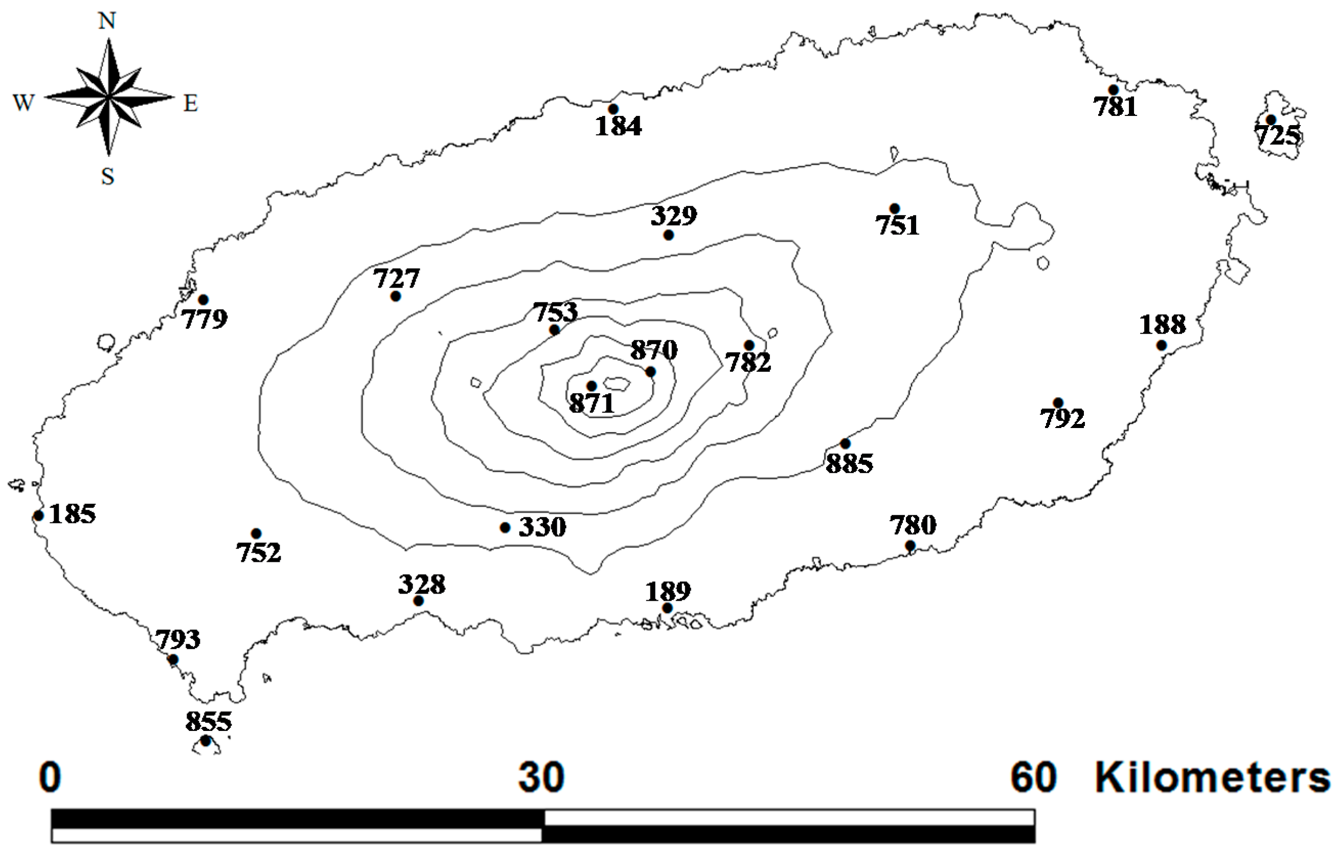
The Jeju Island is a volcanic island that is composed of about 360 small-scale volcanoes and volcanic cones [12]. The Hallasan Mountain is located at the center of the Jeju Island, and sits at a height of 1950 m. The Hallasan Mountain has a gentle slope of about 3° along the east-west direction, but a steeper slope of about 5° along the north-south direction (Jeju Special Self-Governing Province, http://www.jeju.go.kr). The shape of the island is elliptical, with a major axis length of 73 km along the east-west direction and a minor axis length of 31 km along the north-south direction. The total area of the Jeju Island is 1848 km2, and the coastal area whose altitude above sea level is less than 200 m covers 55.3% of the island’s total area.
2.2. Radars
The Korea Meteorological Administration (KMA) operates two radar systems-the Gosan and the Seongsan. The Gosan Radar, which was originally a C-band radar, started tracking typhoons in 1991, but was replaced by an S-band radar in 2006. The Seongsan Radar was introduced in 2006 to supplement the Gosan Radar; in particular, to remove the blind spot that was caused by the Hallasan Mountain. The Seongsan Radar is also an S-band radar. Both possess an observation radius of 240 × 240 km and a resolution of 1 × 1 km. The major specifications of the Gosan and Seongsan Radars are summarized in Table 1.
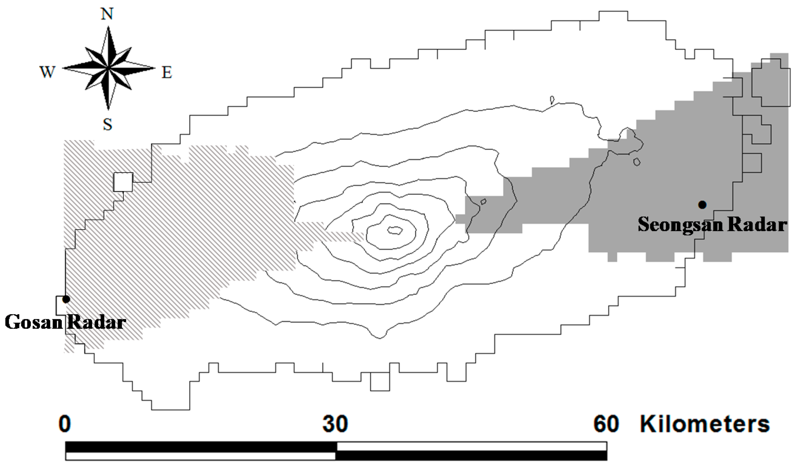
The locations of the Gosan and Seongsan Radars and their radar beam blocking (masking) areas are shown in Figure 2. The radar blocking area in this figure represents the 1.5 km CAPPI (constant altitude plan position indicator) data. Using both of the radars, it is possible to observe the entire island.
2.3. Rain Gauges
In 1990, KMA started to introduce the AWSs in the Jeju Island [2]. Now, 24 AWSs are being operated [8]. Among them, a total of 16 rain gauges are located in the coastal area whose altitude is less than 250 m, four in between 250~500 m, two in between 750~1000 m, one in between 1250~1500 m, and one at 1500 m or higher. The locations of the rain gauges are presented in Figure 3. As can be seen from this figure, the rain gauges are well-distributed over the Jeju Island. That being said, more than half of the total rain gauges are located in the coastal region (0–250 m), and relatively less in the mountainous area. Also, more rain gauges are located on the northern slope of the Hallasan Mountain than the southern slope, which is due to the steepness of the southern slope.
3. Typhoon Nakri
The rainfall event that is considered in this study is the Typhoon Nakri, the 12th typhoon in 2014. The Typhoon Nakri was developed in the Pacific Ocean near the Philippines on 30 July, and arrived at the Jeju Island on 1 August [13]. Originally a mid-sized typhoon, the Typhoon Nakri had become very weak, nearly downgraded to a tropical depression. However, the impact of the Typhoon Nakri was enormous, especially on the Jeju Island. After passing the island, it became a tropical depression on 3 August.
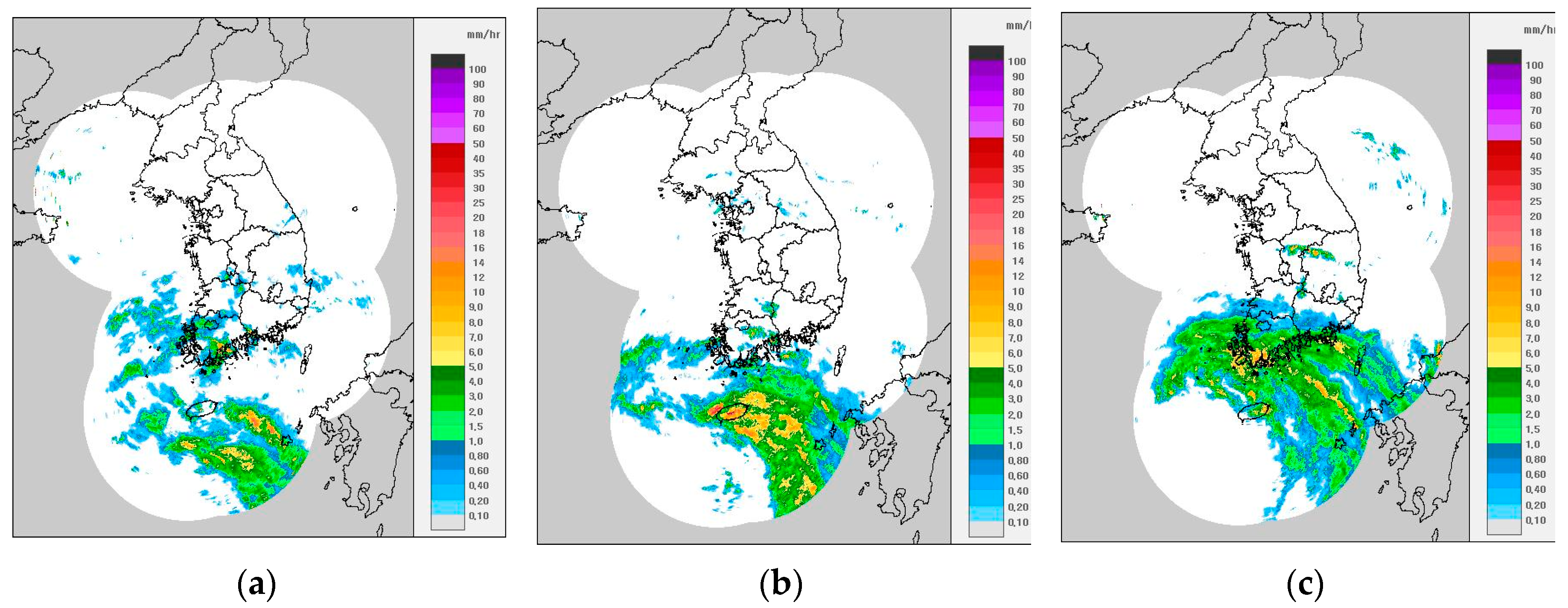
As Typhoon Nakri approached Jeju Island, the central pressure and maximum wind velocity of the Typhoon Nakri were 980 hpa and 25 m/s, respectively. Figure 4 displays the synthetic image of the radar observed on the Korean Peninsula. As can be seen from the figure, the storm center moved from the Jeju Island at 0000 LST (local standard time; LST = UTC + 9 h) 2 August to the southern province of the Korean Peninsula at 0900 LST on the same day.
4. Decision of Z-R Relation at Each Altitude Zone
4.1. Z-R Relations
The Z-R relation is used to estimate the radar reflectivity into the rain rate. Radar measures the intensity of the echo generated from the raindrops in the air, which is the radar reflectivity (Z, mm6/m3), which can also be expressed in decibels (dBZ).
Zero dBZ represents the radar reflectivity if a single raindrop with a diameter of 1 mm is located in a unit volume of 1 m3 [14]. If the information about the drop size distribution (DSD) is given, then Z is calculated as:
In this equation, D represents the diameter of a raindrop, N(D) is the number of raindrops with diameter (D ~ D + dD) in the unit volume. Using the relation between the radar reflectivity and rain rate, one can estimate the rain rate with a given radar reflectivity factor [15]. This is called the Z-R relation, which is:
where, R is the rain rate (mm/h) measured by the rain gauge, and A and b are parameters to be estimated using the observed data.
As can be seen in the above equations, the DSD affects much on the Z-R relation. In case that the rain rate (R) is the same, the radar reflectivity (Z) can be a different value depending on the DSD. In fact, the Z-R relation given in Equation (3) was derived based on that the DSD follows the exponential distribution [16]. The gamma distribution is also frequently considered in the theoretical analysis of Z-R relation [17].
The parameters of the Z-R relation can vary from storm to storm, due to the difference in their DSD distributions [18,19]. In the early studies, the parameters were estimated by considering the fact that the DSD varies according to the storm type [16,20,21,22,23]. It is also possible that both convective and stratiform clouds coexist, and that raindrops evaporate or collide while they are falling to the ground [24].
4.2. Preparation of Radar Reflectivity Data
From both the Gosan and Seongsan radars, a total of eight radar reflectivity fields were prepared from an altitude of 250 m to 2000 m, in intervals of 250 m. These data were used to make the composite field at each altitude. When data were available from both radar systems, their arithmetic mean was calculated to make the representative reflectivity.
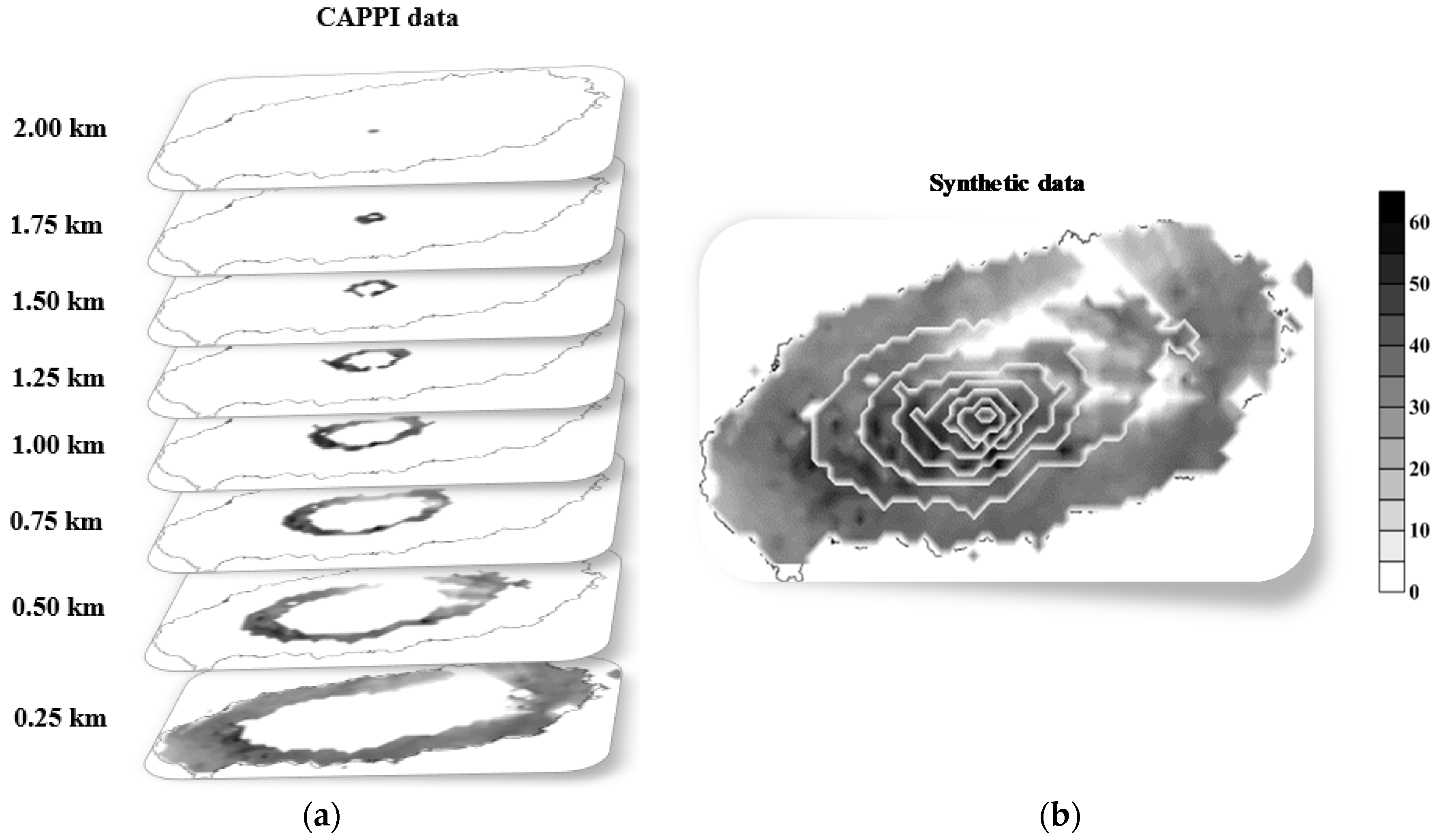
Every 10 min, eight radar composite reflectivity fields were prepared and used to create the ground-level composite reflectivity field for the entire Jeju Island. Figure 5 shows how the ground-level radar composite reflectivity field for the entire Jeju Island was constructed. At each altitude zone from 250 m to 2000 m, only the corresponding-altitude radar CAPPI data were used to make the ground-level radar composite reflectivity field. As the altitude increases, a much smaller toroidal radar CAPPI data field was selected (Figure 5a). Finally, by combining these donut-shaped fields, the full ground-level radar composite reflectivity field over the entire island could be created (Figure 5b). The radar reflectivity values in this figure are all within a maximum altitude difference 250 m to the ground.
4.3. Parameter Estimation of Z-R Relation
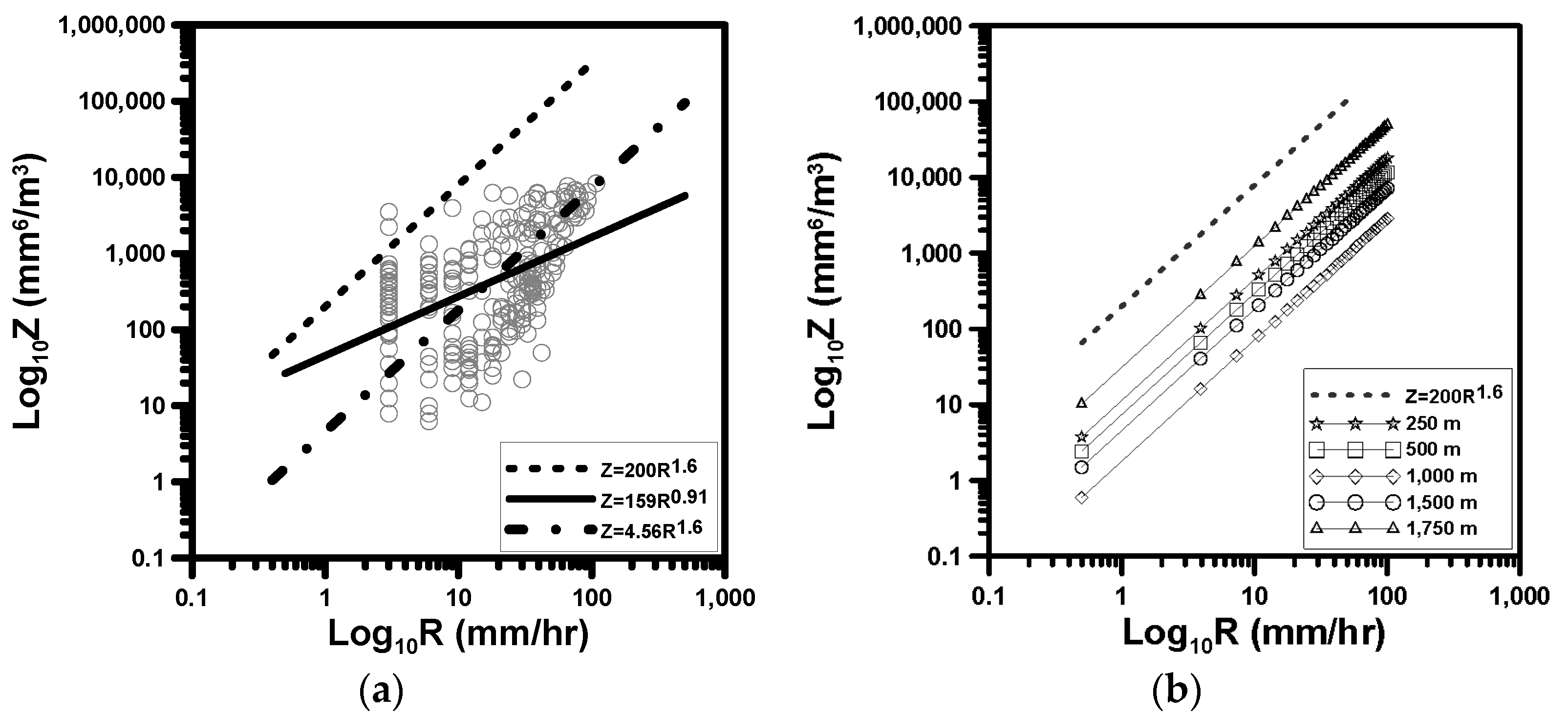
In this study, the Z-R relation was derived independently for each altitude zone; hence, the Z-R relation at one altitude zone (for example, 0–250 m) can differ from that at another (for example, 750–1000 m). Figure 6a shows the resulting Z-R relations that were derived for the altitude zone 1250–1500 m as an example, among which, the solid line represents the one derived without any constraints, and the alternated long and short dash line the one with a fixed exponent b = 1.6 as in Equation (3). The use of the exponent b = 1.6 was based on the visual comparison between the Marshall-Palmer equation [16] and the regression line derived simply by applying the least square method, i.e., . The Marshall-Palmer equation for the stratiform rainfall event, that is, , is also given by the dotted line in the figure for reference. By comparing these two lines on log-log paper, it was found that the slope of the regression line was closer to 1.6. Finally, after fixing the exponent to be 1.6, the new regression line was derived.
As can be seen in this figure, the Z-R relation derived in this study (without any constraints) was very different from the Marshall-Palmer equation with different parameters A and b. However, as the exponent b = 1.6 appeared to be reasonable for the data in this study, only the parameter A was estimated again after fixing b = 1.6. The resulting Z-R relation was found to better fit the observed data, which is also given in the same figure. The exponent b = 1.6 was found to be a reasonable choice for the Z-R relation in all of the altitude zones in this study. Simply by changing the parameter A, the Z-R relation for each altitude could be effectively fit. This parameter estimation was repeated for five altitudes, 250 m, 500 m, 1000 m, 1500 m and 1750 m. For three altitudes −750 m, 1250 m, and 2000 m-the parameter estimation could not be completed due to the absence of rain gauge data. Finally, the Z-R relations derived for each altitude are compared in Figure 6b.
The Z-R relation derived for each altitude zone during the Typhoon Nakri were also found to differ dramatically, as can be seen in Figure 6b. It was also found that the parameter A was, in all of the cases, much smaller than that of the Marshall-Palmer equation. This result indicates that the rain rate is much higher as compared to the strength of radar reflectivity.
When comparing the Z-R relation with the parameter A, it was least at an altitude around 1000 m, and greatest at an altitude around 1750 m. More interestingly, the parameter A from the coastal area (low altitude zone) to the mountain area (high altitude zone) did not show an increasing or decreasing trend. The parameter A was decreased after passing the coastal region, with a minimal value at an altitude around 1000 m, and then increased again. As the change in the parameter A is so large, from 11.4 to 1.8, and then 31.1, it cannot be regarded as a problem from observed data or parameter estimation. On the other hand, this change may be explained by the sea-breeze front [25], which, in general, occurs in the coastal area. As the sea-breeze includes the ascending air current, a convective cloud can be developed easily when the humidity is high. The orographic effect may be the reason to increase the parameters A in the high altitude zone. The rainfall intensity can be increased due to the ascending air current following the mountain slopes, which can also be strengthened when the humidity and wind velocity are all high [26,27,28,29,30,31].
For those altitude zones in which rain gauges are not available, the parameter A was estimated by considering the trend of As, as decided in five altitude zones. The parameter A for the altitude zones of 500–750 m, 1000–1250 m and 1750–2000 m were estimated to be 5.0, 3.2, and 57.7, respectively.
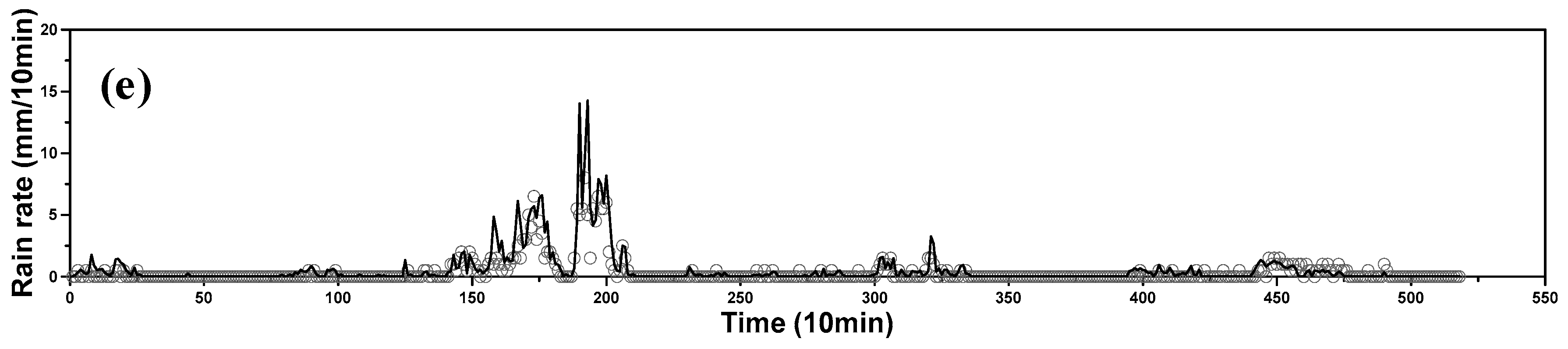
Using the Z-R relations that are determined in this section, the radar rain rate was estimated every 10 min and compared with the rain gauge rain rate (Figure 7). As can be seen in Figure 7, the radar rain rate is sometimes higher or lower than the rain gauge rain rate; however, these rates typically match well. Thus, in this study, the parameters of the Z-R relation were assumed to be properly determined.
4.4. Removal of Abnormal Reflectivity Data
Though the radar and rain gauge rain rate typically match well, there were still some strangely high or low radar rain rates when compared with the surrounding values. It is also from the very high or low radar reflectivity data (hereafter, it is called the abnormal reflectivity). In this study, this abnormal reflectivity was removed by comparing it with surrounding reflectivity values within 3 km range. Figure 8 displays an example for the Witse Oreum AWS station located in the altitude zone of 1500–1750 m. Figure 8a shows the numbers of cells located within the 3 km range around the Witse Oreum AWS station (cell number 7). Since cell number 7 is located in the altitude zone 1500–1750 m, just a few cells are within a 3 km range at the same altitude level and other cells are located at other altitude zones of 1250–1500 m or 1750–2000 m. These cells were excluded in the comparison.
Figure 8b is a scatter plot between the reflectivity at cell number 7 and reflectivity values at other cells within a 3 km range. This shows that the reflectivity at cell number 7 has a 1:1 relation, for the most part, in comparison to the other cells. However, it is also true that some of them exist far from the 1:1 line, even some of the data are concentrated along the X and Y axes, which were assumed abnormal in this study.
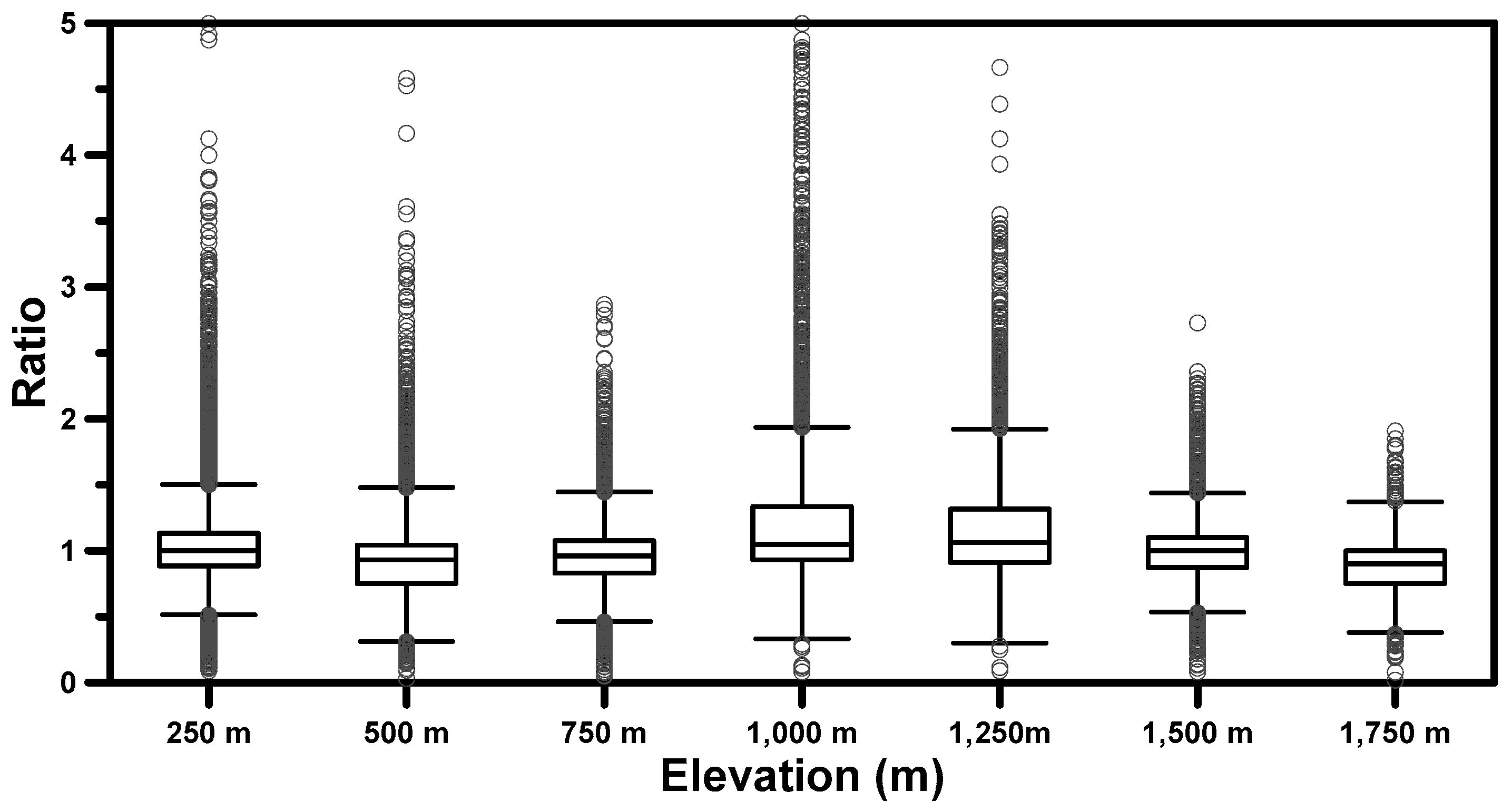
Because it was difficult to distinguish one radar reflectivity as abnormal, a threshold value was derived as the ratio between two adjacent reflectivity values. After summarizing the ratio data by a box-plot for each altitude zone, the values beyond the 1.5 × IQR (interquartile range) were assumed to be abnormal. Figure 9 displays the box-plots rendered for each altitude zone. Reflectivity values that were abnormally higher and lower than surrounding values based on the 1.5 × IQR were all removed. Finally, the removed reflectivity data were filled by the average reflectivity of the surrounding eight cells.
It should also be mentioned that this method of finding and correcting the abnormal values could introduce another type of bias in the resulting reflectivity field. Especially, some of very high reflectivity values can be smoothed out even though they are real. As a result, the maximum rainfall depth to be derived in the following section can be a bit underestimated. However, at this moment, the authors had no choice and expected the results to be statistically reasonable.
5. Maximum Rainfall Depth Records in the Radar Rain Rate Field
5.1. Estimation of Radar Rain Rate Field and G/R Correction
The Z-R relation derived in Section 4 was applied to estimate the radar rain rate field over the Jeju Island. However, at certain times, the radar and rain gauge rain rate still differ dramatically. This disparity, or the mean-field-bias, becomes even larger when the rain rate approaches its maximum. The mean-field-bias correction is the procedure to correct the mean difference between the radar rain rate and the rain gauge rain rate. Generally, the ratio of the means of the rain gauge rain rate and radar rain rate (that is, the G/R ratio) is used for this purpose [32,33]. As the G/R ratio can be estimated easily and in real-time, it has been widely used for the purpose of mean-field bias correction [18,34,35,36]. In this study, the radar rain rate was once again corrected by applying the G/R ratio that was derived at every point of time and for each altitude zone. The G/R ratio was determined by the following equation:
where represents the rain gauge rain rate and the radar rain rate. Additionally, n is the number of data pairs.
The estimated G/R ratios in this study were all around 0.66–1.35. Figure 10 shows the comparison of radar and rain gauge rain rate before and after the G/R correction at some locations of AWSm such as Witse-Oreum (1750 m), Jindallebat (1500 m), Seongpanak (1000 m), Seonheul (500 m), and Seoqwipo (250 m). As can be seen in Figure 10, the G/R correction improved the radar rain rate so that it is similar to the rain gauge rain rate. At some locations, like at Witse-Oreum, the radar rain rate was increased after the G/R correction, while at other locations, like Seongpanak, Seonheul, and Seoqwipo, the radar rain rate was decreased. It was also found that at some locations, like Jindallebat, the radar rain rate still differed from the rain gauge rain rate. Interestingly, at Jindallebat, the radar rain rate was much higher than the rain gauge rain rate before the peak rain rate, but much smaller after the peak rain rate. As a result, the estimated G/R ratio was nearly 1.0, thus the G/R correction could not fix this problem.
5.2. Comparison of Maximum Rainfall Depths and Occurrence Spots
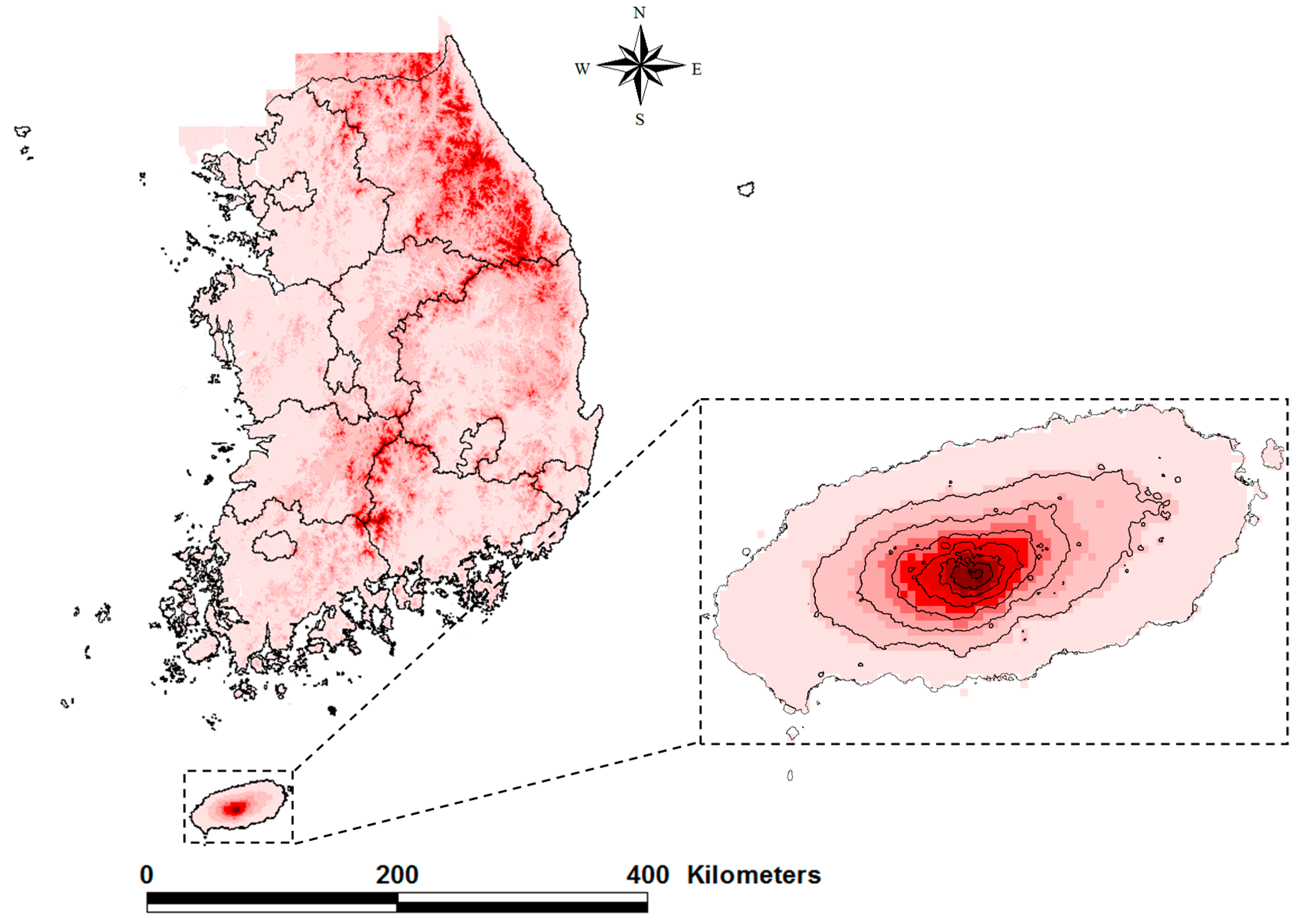
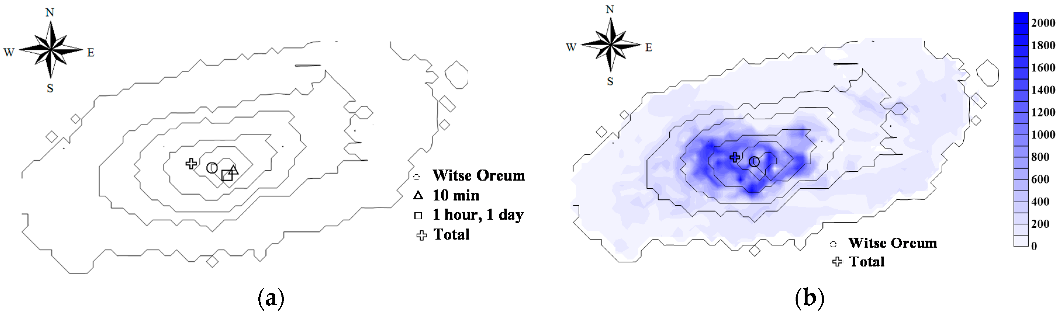
As there are only a few rain gauges available over the Jeju Island, we cannot be sure that the maximum rain rate observed by the rain gauge is truly accurate. Hence, the maximum rainfall depth for some given duration, as well as its spatial region of occurrence, was explored using the radar data prepared in the previous section. The durations of rainfall considered in this study were 10 min, one hour, one day, and the entire period of the Typhoon Nakri. The AWS records show that the maximum rainfall depths for these durations were all recorded at the same location, Witse Oreum.
First, for the duration of 10 min, the maximum rainfall depth was recorded on the opposite side (at a similar altitude) of the Halla Mountain to the location of Witse Oreum (Figure 11). The radar rainfall depth recorded was 67.6 mm, which was about twice as large as the rain gauge measurement of 30.0 mm at Witse Oreum. The occurrence time was also significantly different as the radar measurement was made at 0000 LST 2 August, but the AWS measurement at 0650 LST same day.
Second, for the duration of one hour, the maximum rainfall depth was also recorded on the opposite side of Witse Oreum (Figure 11), but it differs from the location at which the 10-min maximum rainfall depth was recorded. In particular, this location is known to be the steepest side of the Halla Mountain. The radar rainfall depth recorded was 192.0 mm, which was about 50% higher than the rain gauge measurement of 138.0 mm. Its occurrence time was the same as that of the rain gauge measurement at 0700 LST 2 August. For the duration of one day, the maximum rainfall depth was recorded at the same location as that for the one-hour maximum rainfall. The maximum one-day rainfall was observed on 2 August by both the radar and rain gauge. The radar rainfall depth recorded was 1547.3 mm, which was about 30% higher than the rain gauge measurement of 1182.0 mm.
Finally, for the entire duration of the Typhoon Nakri, the maximum rainfall depth was recorded on its west side of Witse Oreum, at same side of the Hallasan Mountain. The altitude of this location was also a bit lower than that of Wirse Oreum. The radar rainfall depth recorded was 1976.8 mm, which was less than 10% different from that of the rain gauge measurement, namely 1734.5 mm. The total duration of rainfall recorded was 88 h. Table 2 summarizes the above maximum rainfall depth for several durations measured by the rain gauge and radar.
6. Conclusions
In this study, radar data was analyzed to investigate the rain rate field over the Jeju Island during the rainfall event that was generated by the Typhoon Nakri in 2014. First, the Z-R relation to convert the radar reflectivity data into rain rate data was developed for each altitude zone (eight altitude zones from 0 to 2000 m in 250 m intervals), which was to consider the possible orographic effect of the Hallasan Mountain in the Jeju Island. After additional data processing to remove outliers and correct the mean-field-bias, the maximum rainfall depths for several durations-0 min, one hour, and one day-were estimated and compared with those measured by the rain gauges. The occurrence spots of those maximum rainfall depths were also determined and compared with those that were recorded by the rain gauges. The results is summarized as follows.
First, the Z-R relation derived for each altitude zone during the Typhoon Nakri shows that the parameter A decreased after passing the coastal region, with a minimal value at an altitude around 1000 m, and then increased again. This change could be explained partly by the sea-breeze front, and partly by the orographic effect.
Second, the spot of maximum rainfall depth over the radar rain rate field was found to be very different from that of rain gauge rain rate field. In particular, the spatial regions of maximum rainfall depth in the radar rain rate field were found to be located near the steepest side of the Hallasan Mountain. There is no rain gauge that is available in this steepest area, but one on the opposite side of the Hallasan Mountain, Witse Oreum.
Third, it was also found that, especially for the rainfall duration of 10 min, the occurrence time of the maximum rainfall depth that was recorded by the radar rain rate data was different from the rain gauge rain rate data. Their locations differed as well. However, the occurrence time was the same for the long rainfall duration, like one day.
Finally, the maximum rainfall depths recorded by the radar were found to be higher than the rain gauge by 10% (entire duration) to 100% (10 min). As the rain gauge data are available only at several locations, the true maximum rainfall depth for a given rainfall duration must be greater than that observed by the rain gauge. In that sense the maximum rainfall depths recorded by the radar can be assumed to be reasonable, and the radar data can be used to perform a more detailed investigation of the rain rate field over a region as in this study.
Acknowledgments
This research was supported by the ‘Basic Science Research Program’, through the National Research Foundation of Korea, funded by the Ministry of Education (NRF-2016R1D1A1A09918155).
Author Contributions
All the authors contributed in the writing of the paper.
Conflicts of Interest
The authors declare no conflict of interest.
References
- Um, M.-J.; Cho, W.; Rim, H.-W. Rainfall adjustment on duration and topographic elevation. J. Korea Water Resour. Assoc. 2007, 40, 511–521. [Google Scholar] [CrossRef]
- Choi, G. Spatial patterns of seasonal extreme precipitation events in Mt. Halla. KU Clim. Res. Inst. 2013, 8, 267–280. [Google Scholar] [CrossRef]
- Jeju Regional Office of Meteorology. Regional Climate Change Report (Jeju Island); Jeju Regional Office Meteorology: Jeju, Korea, 2011; pp. 21–25.
- Dore, A.J.; Choularton, T.W. Orographic rainfall enhancement in the mountains of the Lake District and Snowdonia. Atmos. Environ. 1992, 26, 357–371. [Google Scholar] [CrossRef]
- Misumi, R. A study of the heavy rainfall over the Ohsumi Peninsula (Japan) caused by Typhoon 9307. J. Meteorol. Soc. Jpn. 1996, 74, 101–113. [Google Scholar] [CrossRef]
- Suprit, K.; Shankar, D. Resolving orographic rainfall on the Indian west coast. Int. J. Climatol. 2008, 28, 643–657. [Google Scholar] [CrossRef]
- White, A.B.; Nieman, P.J.; Ralph, F.M.; Kingsmill, D.E.; Persson, P.E.G. Coastal orographic rainfall processes observed by radar during the California Land-Falling Jets Experiment. J. Hydrometeorol. 2003, 4, 264–282. [Google Scholar] [CrossRef]
- National Geographic Information Institute. The Geography of Korea—Jeju Special Self-Governing Province; National Geographic Information Institute: Suwon-si, Korea, 2013.
- Korea Meteorological Administration. 40 Years History of Weather Radar in Korea; Korea Meteorological Administration: Seoul, Korea, 2012; pp. 96–97.
- Yu, C.K.; Cheng, L.W. Radar observations of intense orographic precipitation associated with Typhoon Xangsane (2000). Mon. Weather Rev. 2008, 136, 497–521. [Google Scholar] [CrossRef]
- Smith, R.B.; Schafer, P.; Kirshbaum, D.J.; Regina, E. Orographic precipitation in the tropics: Experiments in Dominic. J. Atmos. Sci. 2009, 66, 1698–1716. [Google Scholar] [CrossRef]
- Jeju Regional Office Meteorology. Detailed Climate Characteristics of Jeju Island; Jeju Regional Office Meteorology: Jeju, Korea, 2010; pp. 9–10.
- National Typhoon Center. Typhoons Affecting the Korean Peninsula; Analysis Report; National Typhoon Center: Jeju, Korea, 2015; pp. 73–74.
- Lee, J.; Ryu, C. Radar Meteorology; Sigmapress: Busan, Korea, 2009; pp. 73–74. [Google Scholar]
- Bringi, V.N.; Chandrasekar, V. Polarimetric Doppler Weather Radar, Principles and Applications; Cambridge University Press: Cambridge, UK, 2001; pp. 534–537. [Google Scholar]
- Marshall, J.S.; Palmer, W.M. The distribution of raindrop with size. J. Atmos. Sci. 1948, 5, 165–166. [Google Scholar] [CrossRef]
- Ulbrich, C.W. Natural variations in the analytical form of the raindrop size distribution. J. Clim. Appl. Meteorol. 1983, 22, 1764–1775. [Google Scholar] [CrossRef]
- Chumchean, S.; Seed, A.; Sharma, A. Correcting of real-time radar rainfall bias using a Kalman filtering approach. J. Hydrol. 2006, 317, 123–137. [Google Scholar] [CrossRef]
- Smith, J.A.; Seo, D.J.; Baeck, M.L.; Hudlow, M.D. An intercomparison study of NEXRAD precipitation estimates. Water Resour. Res. 1996, 32, 2035–2045. [Google Scholar] [CrossRef]
- Jones, D.M.A. Rainfall Drop-Size Distribution and Radar Reflectivity; Research Report 6; Illinois State Water Survey: Urbana, IL, USA, 1956; pp. 3–5. [Google Scholar]
- Battan, L.J. Radar Observation of the Atmosphere; The University of Chicago Press: Chicago, IL, USA, 1973; p. 324. [Google Scholar]
- Blanchard, D.C. Raindrop size distribution in Hawaiian rains. J. Meteorol. 1953, 10, 457–473. [Google Scholar] [CrossRef]
- Twomey, S. On the measurement of precipitation intensity by radar. J. Meteorol. 1953, 10, 66–67. [Google Scholar] [CrossRef]
- Jung, S.H.; Kim, K.E.; Ha, K.J. Real-time estimation of improved radar rainfall intensity using rainfall intensity measured by rain gauges. Asia-Pac. J. Atmos. Sci. 2005, 41, 751–762. [Google Scholar]
- Aguado, E.; Burt, J.E. Understanding Weather and Climate, 4th ed.; Pearson: Hoboken, NJ, USA, 2005; pp. 182–187. [Google Scholar]
- Alter, J.C. Normal precipitation in UTAH. Mon. Weather Rev. 1919, 47, 633–636. [Google Scholar] [CrossRef]
- Barrows, H.K. Precipitation and runoff and altitude relations for Connecticut River. EOS Trans. Am. Geophys. Union 1933, 12, 396–406. [Google Scholar] [CrossRef]
- Henry, A.J. Increase of precipitation with altitude. Mon. Weather Rev. 1919, 47, 33–41. [Google Scholar] [CrossRef]
- Hutchinson, P. An analysis of the effect of topography on rainfall in the Taieri Catchment area, Otago. Waikato Geol. Soc. Univ. Waikato 1968, 2, 51–68. [Google Scholar]
- Schermerhorn, V.P. Relations between topography and annul precipitation in western Oregon and Washington. Water Resour. Res. 1967, 3, 707–711. [Google Scholar] [CrossRef]
- Spreen, W.C. A determination of the effect of topography upon precipitation. Trans. Am. Geophys. Union 1947, 28, 285–290. [Google Scholar] [CrossRef]
- Yoo, C.; Yoon, J. A proposal of quality evaluation methodology for radar data. KSCE J. Civ. Eng. 2010, 30, 429–435. [Google Scholar]
- Smith, J.A.; Krajewski, W.F. Estimation of the mean field bias of radar rainfall estimates. J. Appl. Meteorol. 1991, 30, 397–412. [Google Scholar] [CrossRef]
- Seo, D.J.; Breidenbach, J.P.; Johnson, E.R. Real-time estimation of mean field bias in radar rainfall data. J. Hydrol. 1999, 223, 131–147. [Google Scholar] [CrossRef]
- Anagnostou, E.N.; Krajewski, W.F. Real-time radar rainfall estimation. Part I: Algorithm formulation. J. Atmos. Ocean. Technol. 1999, 16, 189–197. [Google Scholar] [CrossRef]
- Chumchean, S.; Sharma, A.; Seed, A. Radar rainfall error variance and its impact on radar rainfall calibration. Phys. Chem. Earth 2003, 28, 27–39. [Google Scholar] [CrossRef]
Figure 1.
Location of the Jeju Island, Korea (the contour lines over the Jeju Island represent the 250 m altitude interval).
Figure 1.
Location of the Jeju Island, Korea (the contour lines over the Jeju Island represent the 250 m altitude interval).

Figure 2.
Location of the Gosan and Seongsan radars and their beam blocking areas (shaded area and hatched area, respectively) for the 1.5 km CAPPI.
Figure 2.
Location of the Gosan and Seongsan radars and their beam blocking areas (shaded area and hatched area, respectively) for the 1.5 km CAPPI.

Figure 3.
Rain gauges over the Jeju Island (Among them, the rain gauge #871 (Witse Oreum) recorded the daily rainfall of 1182 mm during the Typhoon Nakri in 2014).
Figure 3.
Rain gauges over the Jeju Island (Among them, the rain gauge #871 (Witse Oreum) recorded the daily rainfall of 1182 mm during the Typhoon Nakri in 2014).

Figure 4.
Synthetic radar image around the Korea Peninsula during the Typhoon Nakri in the Jeju Island (2 August 2014). (a) 2014/08/02/00:00; (b) 2014/08/02/06:00; (c) 2014/08/02/12:00.
Figure 4.
Synthetic radar image around the Korea Peninsula during the Typhoon Nakri in the Jeju Island (2 August 2014). (a) 2014/08/02/00:00; (b) 2014/08/02/06:00; (c) 2014/08/02/12:00.

Figure 5.
Construction of ground-level radar reflectivity field over the Jeju Island using the radar CAPPI (radar data observed on 0500 LST 2 August 2014). (Each altitude zone radar CAPPI data (a), and the radar composite reflectivity field over the entire island (b)).
Figure 5.
Construction of ground-level radar reflectivity field over the Jeju Island using the radar CAPPI (radar data observed on 0500 LST 2 August 2014). (Each altitude zone radar CAPPI data (a), and the radar composite reflectivity field over the entire island (b)).

Figure 6.
Z-R relations determined for the altitude zone 1250–1500 m as an example (a), and those determined for each altitude zone (b). (In Figure 6a represents the Z-R relation proposed by Marshall and Palmer (1948), the regression equation derived simply by applying the least square method, and the one derived after fixing the exponent b to be 1.6).

Figure 7.
Comparison of radar and rain gauge rain rate at several AWS locations (a) #871 (Witse-Oreum, 1750 m); (b) #870 (Jindallebat, 1500 m); (c) #782 (Seongpanak, 1000 m); (d) #751 (Seonheul, 500 m); and (e) #189 (Seoqwipo, 250 m).
Figure 7.
Comparison of radar and rain gauge rain rate at several AWS locations (a) #871 (Witse-Oreum, 1750 m); (b) #870 (Jindallebat, 1500 m); (c) #782 (Seongpanak, 1000 m); (d) #751 (Seonheul, 500 m); and (e) #189 (Seoqwipo, 250 m).


Figure 8.
Cells around Witse Oreum (cell number 7) (a), and the scatter plot of radar reflectivity data at Witse Oreum and nearby cells within 3 km range (b).
Figure 8.
Cells around Witse Oreum (cell number 7) (a), and the scatter plot of radar reflectivity data at Witse Oreum and nearby cells within 3 km range (b).
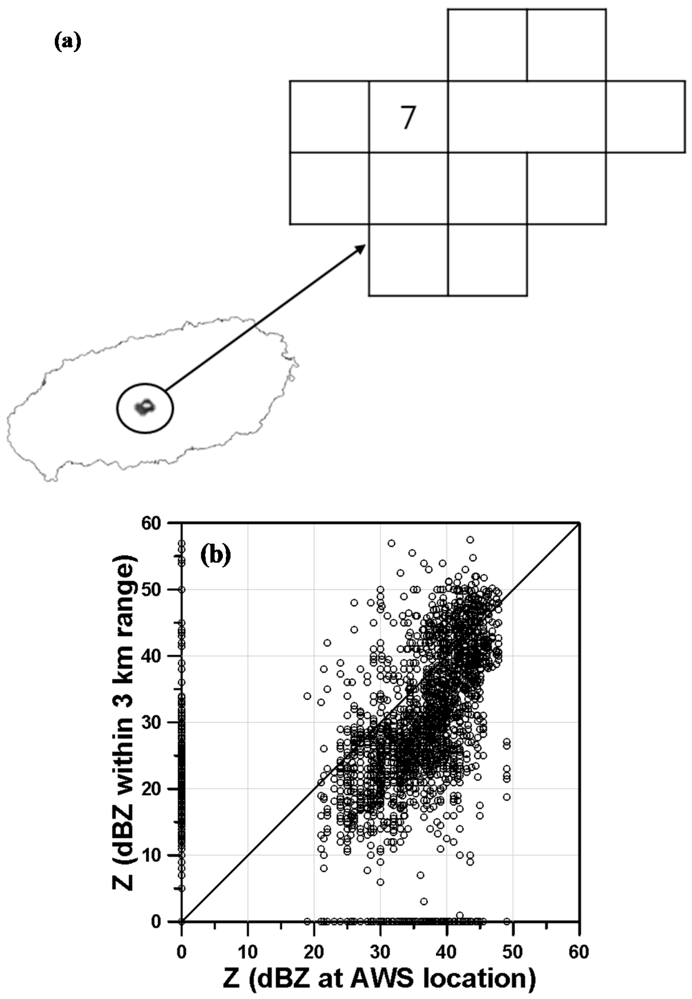
Figure 9.
Box plots of radar reflectivity ratio between two adjacent cells derived at each altitude zone.
Figure 9.
Box plots of radar reflectivity ratio between two adjacent cells derived at each altitude zone.

Figure 10.
Comparison of radar and rain gauge rain rate before and after the G/R correction at several AWS locations (a) #871 (Witse-Oreum, 1750 m); (b) #870 (Jindallebat, 1500 m); (c) #782 (Seongpanak, 1000 m); (d) #751 (Seonheul, 500 m); and (e) #189 (Seoqwipo, 250 m).
Figure 10.
Comparison of radar and rain gauge rain rate before and after the G/R correction at several AWS locations (a) #871 (Witse-Oreum, 1750 m); (b) #870 (Jindallebat, 1500 m); (c) #782 (Seongpanak, 1000 m); (d) #751 (Seonheul, 500 m); and (e) #189 (Seoqwipo, 250 m).
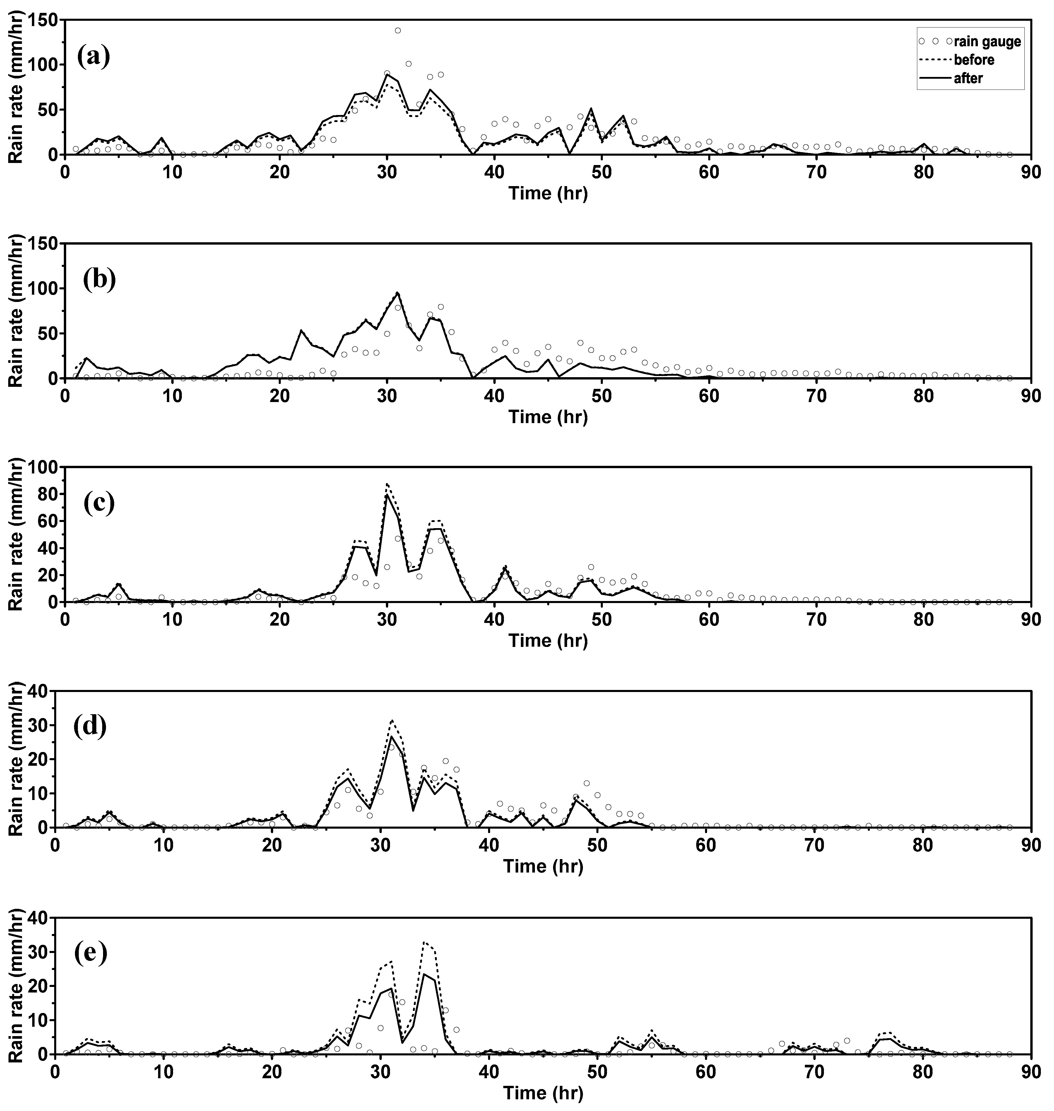
Figure 11.
Locations of maximum rainfall depths for several durations (a) and the spatial distribution of total rainfall depth during the Typhoon Nakri (b).
Figure 11.
Locations of maximum rainfall depths for several durations (a) and the spatial distribution of total rainfall depth during the Typhoon Nakri (b).


Table 1.
Major specification of the Gosan and Seongsan Radars.
| Gosan Radar | Seongsan Radar | ||
|---|---|---|---|
| Radar type | S-band | S-band | |
| Transmitter | Transmitting tube | Klystron | Klystron |
| Receiver | Frequency | 2825 MHz | 2755 MHz |
| Peak Power | 750 kW | 750 kW | |
| Pulse width (short/long) | 1.0/4.5 | 1.0/4.5 | |
| PRF | 250~1200 Hz | 250~1200 Hz | |
| Occupied bandwidth | 8 MHz | 8 MHz | |
| Antenna | Dynamic range | 95 dB | 95 dB |
| Intermediate frequency | 10 MHz | 10 MHz | |
| Antenna diameter | 8.5 m | 8.5 m | |
| Beam width | 1.0° | 1.0° | |
| Antenna gain | 45 dB | 45 dB | |
Table 2.
Comparison of maximum rainfall depths recorded by rain gauge and radar for several rainfall durations.
Table 2.
Comparison of maximum rainfall depths recorded by rain gauge and radar for several rainfall durations.
| Rain Gauge | Radar | |
|---|---|---|
| 10 min | 30.0 mm | 67.6 mm |
| (0650 LST 2 August 2014) | (0000 LST 2 August 2014) | |
| 1 h | 138.0 mm | 192.0 mm |
| (0700 LST 2 August 2014) | (0700 LST 2 August 2014) | |
| 1 day | 1182.0 mm | 1547.3 mm |
| (2 August 2014) | (2 August 2014) | |
| Total | 1734.5 mm | 1976.8 mm |
| (1–3 August 2014) | (1–3 August 2014) |
© 2017 by the authors. Licensee MDPI, Basel, Switzerland. This article is an open access article distributed under the terms and conditions of the Creative Commons Attribution (CC BY) license (http://creativecommons.org/licenses/by/4.0/).
Share and Cite
MDPI and ACS Style
Ku, J.M.; Yoo, C. Calibrating Radar Data in an Orographic Setting: A Case Study for the Typhoon Nakri in the Hallasan Mountain, Korea. Atmosphere 2017, 8, 250. https://doi.org/10.3390/atmos8120250
AMA Style
Ku JM, Yoo C. Calibrating Radar Data in an Orographic Setting: A Case Study for the Typhoon Nakri in the Hallasan Mountain, Korea. Atmosphere. 2017; 8(12):250. https://doi.org/10.3390/atmos8120250
Chicago/Turabian StyleKu, Jung Mo, and Chulsang Yoo. 2017. "Calibrating Radar Data in an Orographic Setting: A Case Study for the Typhoon Nakri in the Hallasan Mountain, Korea" Atmosphere 8, no. 12: 250. https://doi.org/10.3390/atmos8120250
Note that from the first issue of 2016, this journal uses article numbers instead of page numbers. See further details here.