Article

An Evaluation of the CHIMERE Chemistry Transport Model to Simulate Dust Outbreaks across the Northern Hemisphere in March 2014

1
INERIS, National Institute for Industrial Environment and Risks, Parc Technologique ALATA, 60550 Verneuil-en-Halatte, France
2
Laboratoire de Météorologie Dynamique, Ecole Polytechnique, PSL Research University, Ecole Normale Supérieure, Université Paris-Saclay, Sorbonne Universités, UPMC University Paris 06, CNRS, Route de Saclay, 91128 Palaiseau, France
3
Central Laboratory, Beijing Municipal Institute of Labour Protection, Room 317, 55 Taoranting Road, Xicheng District, Beijing 100054, China
4
École des Ponts ParisTech, Université Paris-Est, 77455 Champs-sur-Marne, France
5
Laboratoire d’Aérologie, Université de Toulouse, CNRS, UPS, 14 Avenue Edouard Belin, 31400 Toulouse, France
*
Author to whom correspondence should be addressed.
Atmosphere 2017, 8(12), 251; https://doi.org/10.3390/atmos8120251
Submission received: 22 October 2017 / Revised: 7 December 2017 / Accepted: 8 December 2017 / Published: 13 December 2017
(This article belongs to the Section Air Quality)

Abstract

:
Mineral dust is one of the most important aerosols over the world, affecting health and climate. These mineral particles are mainly emitted over arid areas but may be long-range transported, impacting the local budget of air quality in urban areas. While models were extensively used to study a single specific event, or make a global analysis at coarse resolution, the goal of our study is to simultaneously focus on several affected areas—Europe, North America, Central Asia, east China and the Caribbean area—for a one-month period, March 2014, avoiding any parameter fitting to better simulate a single dust outbreak. The simulation is performed for the first time with the hemispheric version of the CHIMERE model, with a high horizontal resolution (about 10 km). In this study, an overview of several simultaneous dust outbreaks over the Northern Hemisphere is proposed to assess the capability of such modeling tools to predict dust pollution events. A quantitative and qualitative evaluation of the most striking episodes is presented with comparisons to satellite data, ground based particulate matter and calcium measurements. Despite some overestimation of dust concentrations far from emission source areas, the model can simulate the timing of the arrival of dust outbreaks on observational sites. For instance, several spectacular dust storms in the US and China are rather well captured by the models. The high resolution provides a better description and understanding of the orographic effects and the long-range transport of dust plumes.

Graphical Abstract

1. Introduction

Air quality impairment is one of the major environmental threats throughout the world. The impact of pollutants on health, ecosystems and climate were clearly highlighted by many studies. The main sources of pollutants are anthropogenic and biogenic in origin and in the two last decades, particulate matter (PM) were identified as a vector of toxics particularly the fine fractions PM10 and PM2.5 (respectively, the mass of particles with diameter below 10 and 2.5 µm). According to the World Health Organization, in 2012, air pollution was responsible for 7 million premature deaths, 3.7 million deaths from ambient air pollution and 4.3 million deaths from household air pollution [1]. Long-term or short-term exposure to PM10 and PM2.5 could trigger hospital visits for asthma in children, as recently shown in China [2].
At the global level, mineral dust is one of the major species affecting the PM background concentrations, interacting with clouds and then on the radiative budget [3,4] and will also be particularly affected by climate change in the future [5]. The Sahara is certainly the largest source of atmospheric desert dust [6], contributing about 50% of the global total, followed by China and Central Asia (about 20% of the global total), Arabia and Australia. Drylands in Southern Africa and the Americas are relatively minor sources, together accounting for probably less than 5% of the global total. To a lesser extent, large agricultural areas can also contribute to soil PM, a good example is the dust event originated from Ukraine chernozemic soils in 2007 [7]. Health impacts of dust can be illustrated by the case of the Sahel region [8]. This region of West Africa has the highest bacterial meningitis attack and case fatality rates in the world. Mice exposed to the interaction of both heat and dust inhalation have significantly increased risk of invasive pneumococcal disease. It might be that the combination of abrasion of the respiratory tract, impaired phagocytosis, and increased release of damaging pathogen toxins creates a “perfect storm” for dissemination of colonized bacteria from the nasopharynx [9,10]. Moreover, several studies show the impact of natural dust on asthma hospital admissions of affected people [11,12,13,14,15] and the importance of the mix of dust with anthropogenic pollution [16]. Model simulations suggest that global annual dust emissions have increased by 25% to 50% over the last century due to a combination of land use and climate changes. Sand dust storm frequency and severity have increased in recent decades in some areas but decreased in other areas. There appear to have been no major changes in dust activity over the past three decades over North Africa, the Middle East and South America, whereas there have been substantial changes in the US high plains, central Asia and Australia [17]. Over the Northern Hemisphere, the south of Europe, the Caribbean zone, and Central to East Asia are particularly affected by dust outbreaks leading to PM10 exceedances [18,19]. From the Rocky Mountains to the central plains of USA, dust storms can also occur and lead to very high PM concentration levels in these regions with an intensification of dust storms within the last two decades [20,21]. Concentration peaks usually occur in early spring in this region. Atmospheric transport of dust is also the major source of iron and other nutrients in ocean [22,23] and plays an important role on the biogeochemical of marine ecosystems through atmospheric fallouts of dust. Dust storms have economic implications, most usually account for household cleaning and disruption to commercial activities (retail and service industries), air transport and construction [6,7,8,9,10,11,12,13,14,15,16,17,18,19,20,21,22,23,24].
Modeling tools, the so-called chemistry transport models (CTMs), have been designed to work from the global to local scales. While global models used to focus on major species such as primary organic matter, sulfates and desert dust, regional models were better developed to predict the secondary organic and inorganic chemistry. Now, regional and global models host similar chemical and physical modules, only the resolution can differ with still different goals.
Global CTMs are closely linked to long-term simulations related to climate change issues and to predict monthly or annual evolution of the atmospheric composition, they are commonly used at 1° to 2° horizontal resolution to gain computing time. Model forecast of dust outbreaks from Africa to Europe have been evaluated using global and regional chemistry transport models [25]. Models tend to underestimate the long-range transport towards Northern Europe. Their analysis suggests that this is partly due to difficulties in simulating the vertical distribution of dust and horizontal winds. Recently, the NOAA National Centers for Environmental Prediction (NCEP) implemented the NOAA Environmental Modeling System (NEMS) Global Forecast System (GFS) Aerosol Component (NGAC) for global dust forecasting in collaboration with NASA Goddard Space Flight Center (GSFC). NGAC Version 1.0 has been providing five-day dust forecasts at 1° × 1° resolution [26,27].
Regional models are usually run for air quality purposes over short periods such as short term forecasts [28] from the regional up to the urban scales (for large cities) with resolution up to 1 or 2 km over large domains [29] showing the added value of finer resolutions to analyze the evolution of anthropogenic pollution plumes issued from source areas. However, using a finer resolution improves the bias but can lead to an impairment of the spatial correlations if the quality of emissions is not improved appropriately [29]. Regional models are also commonly used for policy analysis with yearly simulation in “scenario modes” [30] or for climate impact studies [31]. The meteorological conditions influencing the development of deep convection, such as mixing depth, local thermodynamic variability, and wind velocity, are best resolved by models having much higher resolution than current global CTMs [32,33]. The added value of a finer resolution is also mentioned for models in other recent studies for the transport of dust in West Asia [34,35]. Differences due to a finer resolution are also associated to the channelization of the dust flow through valleys and the differences in the modeled altitude of the mountains that alters the meteorology and blocks the simulated dust fronts limiting the dust transport. For the USA, the use of the Non Hydrostatic Mesoscale Dust model at fine resolution [36] shows a large improvement of dust storm simulation thanks to the improvement of the quality of input data such as soil moisture and vegetation cover. A major West African dust storm was simulated at 5 km resolution with the French modeling system AROME coupled with the ORILAM aerosol model [37]. A high-resolution modeling of dust phenomena is computationally demanding and requires high-resolution input fields [38], however, high resolution simulations ensure a better quantification of dust source regions, meteorological mechanisms that control dust emission fluxes [39,40], transport pathways [41,42], dust radiative direct and indirect effects, complex atmospheric chemistry, and deposition processes. For anthropogenic pollution, a statistical evaluation performed by [43] showed that the increased resolution better reproduces the spatial gradients in pollution regimes, but does not help to improve significantly the model performance for reproducing observed temporal variability. However, this study clearly shows that increasing model resolution is advantageous, and that leaving a resolution of 50 km in favor of a resolution between 10 and 20 km is practical and worthwhile. For ozone, a horizontal resolution of 12 km was considered as an optimum value to simulate the concentrations over the Paris Basin [44]. For dust storms, the intermediary spatial scale of about 100 km to about 1000 km consistent with ranges in between local and regional scales is critical and crucial to analyze because many population centers lie on the margins of deserts and because large amounts of dust can be transported over these intermediate distances, these regional dust-transport events are rarely documented as discussed in [45].
The development of global emission inventories resulting of the merge of continental emission inventories authorizes the global and regional models to be used at the same resolution over large domains. Thus, recently the CHIMERE model has been developed to work at the hemispheric level at 10 km resolution consistently with global existing emission inventories [46]. Several numerical issues have been solved to reach this goal and a work has been carried out to improve the emission of mineral dust throughout the world either from arid and semi-arid areas or from large dried arable lands.
In this study, a high spatial resolution simulation (about 10 km) for a one-month period (March 2014) over the Northern Hemisphere was performed with the last CHIMERE version [46]. Spring is known to be one of the more active seasons for dust emissions in the Northern Hemisphere [47]. This complete simulation including anthropogenic pollution and natural species including windblown dust emissions is an opportunity to evaluate the ability of the model to simulate the transport of mineral dust plumes far from emission sources at very fine resolution throughout the Northern Hemisphere. While models were extensively used to study a single specific event, or make a global analysis at coarse resolution, the goal of our study is to simultaneously focus on several areas—Europe, North America, Central Asia, east China and the Caribbean area—for a one-month period. After an overview of modeled results at the global scale with global budgets related to dust concentrations and their transport, a quantitative and qualitative evaluation of the most striking episodes over the five previously identified areas will be performed using satellite data and ground based PM and calcium measurements where available. The results are analyzed in the context of the previous studies related to these episodes; the fine resolution of the simulation authorizes local scale analyzes of some local specific features.

2. Experiments

2.1. Modeling Tools

2.1.1. The Chemistry Transport Model CHIMERE

The CHIMERE off-line chemistry transport model [46,48] was used to model the transport and transformation of trace species in the lower troposphere. Several international teams for research and environmental policy underpinning are using the model. It has been involved in several model inter-comparison initiatives [49,50,51,52,53,54] and is now a part of the COPERNICUS services (Available online: http://www.copernicus.eu). The model and further documentation can be found at http://www.lmd.polytechnique.fr/chimere/. Simulations at very high resolution have been performed over domains encompassing the full European domain [29,55] with resolutions up to 2 km thanks to refined emission inventories using adequate proxies for emission regridding. Besides the technical challenge, the authors found that model biases were significantly reduced, especially over urban areas. The high-resolution grid also allows reevaluating the contribution of individual city plumes to the European burden of pollution, providing new insights to target the appropriate geographical level of action when designing air pollution mitigation strategies. The CHIMERE 2017 version [46] has been used in this study. Several improvements to work at the hemispheric level on the parallelization, numeric schemes, deposition processes, mineral dust emissions (described in next section), chemistry and physics of the aerosols (condensation and coagulation processes) have been performed. Particularly, the notion of wet diameter and wet density was introduced in CHIMERE-2017. Particles are distributed between bins according to their dry diameter. The wet diameter of the particles is calculated as a function of humidity and the composition of the particle. To compute the wet density and wet diameter for each aerosol size bin, the amount of water in each bins is computed with the “reverse mode” of the thermodynamic module ISORROPIA [56] by using the composition of particles, assuming that only sulfate, nitrate, ammonium and sea salts have a high enough hygroscopicity to absorb a significant amount of water. The density of the aqueous phase of particles is computed according to composition following the method in [57].

2.1.2. Model Set-Up

The model grid covers the Northern Hemisphere using a polar stereographic projection with 1440 × 1440 points. With this projection and this number of points, the horizontal model resolution varies from 18 × 18 km2 at the Equator to 9 × 9 km2 at the Pole. Global chemical fields from a six-year reanalysis with the LMDz4-INCA3 model [58,59] are used as boundary conditions for the model top and lateral borders. For this simulation, the lateral boundary conditions (under the Equator) will have a low impact since the selected domain covers the whole Northern Hemisphere with few interactions with Southern Hemisphere.
The vertical discretization has 16 layers extending from approximately 997 hPa to 200 hPa. This number of layers is a compromise between accuracy and computing capability, certainly this is not sufficient to well simulate the long-range transport of pollutants, and this has to be analyzed in follow-up works. The period of March 2014 is simulated with 15 days spin-up in February 2014. The model configuration is summarized here, but the reader is referred to the reference CHIMERE publication [46] for details on the corresponding model components and references as well as non-user-specific model characteristics. The gas-phase chemical mechanism is MELCHIOR2, which consists of a simplified version (40 species and 120 reactions) of the full chemical mechanism based on the concept of chemical operators. Modeled particulate matter includes primary particulate matter, and secondary inorganic (nitrate, sulfate, ammonium based on the ISORROPIA thermodynamic equilibrium model) and organic aerosol (whose formation is represented according to a single-step oxidation of the relevant anthropogenic and biogenic precursors and gas–particle partitioning of the condensable oxidation products). For the computation of thermodynamic equilibrium, the relative humidity is capped with a maximum value of 97% to avoid a too large growth of particle size. Biogenic emissions are computed with MEGAN version 2.04, sea-salt and mineral dust emissions are also considered, emission parameterization for the latter species is discussed later.
The particle size ranges from 10 nm to 40 µm over 10 bins according these ranges from bin No. 1 to bin No. 10 which are, respectively, 10.00–22.01 nm, 2.20–48.43 nm, 48.43–106.7 nm, 106.7–234.7 nm, 234.7–516.2 nm, 516.2–1.14 µm, 1.14–2.50 µm, 2.5–5.0 µm, 5.0–10.0 µm, and 10–40 µm. In this paper, SIA, SOA, DUST, SALT, and TPPM, respectively, refer to Secondary Inorganic Aerosol (sum of nitrate, sulfate and ammonium), Secondary Organic Aerosols (anthropogenic and biogenic in origins), natural mineral dust, sea salt and Total Primary Particle Matter (total primary anthropogenic carbonaceous and non-carbonaceous species). The attribute “−10”, “−25” or “coarse” are affected, respectively, for the PM10, and PM2.5 and the coarse (PM10–PM2.5) fractions. “Total dust” (sum over all bins including the bin above 10 µm) is a terminology sometimes used in this study; the “coarse” fraction can include the last bin in some analyses.
Horizontal transport is solved with the second-order Van Leer scheme. Subgrid scale convective fluxes are considered. The present set-up also benefits from an improved representation of turbulent mixing in urban areas that yields lower horizontal wind and vertical mixing to better capture the difference between the urban canopy (where the first CHIMERE model level lies) and the top of the urban sublayer of which the lowermost meteorological model level is representative [55].
As an offline CTM, CHIMERE requires prescribed meteorological fields which were provided here by ECMWF with the Integrated Forecasting System model at 0.125° resolution with data assimilation consistent with the CHIMERE horizontal resolution. Emissions for the main pollutants are issued from the EDGAR-HTAP initiative [60,61,62]. The EDGAR-HTAP project compiled a global emission dataset with annual inventories for CH4, NMVOC, CO, SO2, NOx, NH3, PM10, PM2.5, BC (Black Carbon), OC (Organic Carbon) and covering the period 2008–2010 using, to the extent possible, official or scientific inventories at the national or regional scale that are likely to be acceptable for policy makers in each region of the world. This compilation of different official inventories from EMEP for Europe, EPA for USA, GAINS for China and REAS was first gap-filled with global emission data of EDGARv4.2. For this period, the 2010 dataset has been used; monthly emissions of these macro pollutants are pre-processed in the CHIMERE suite to fit with the simulation grid, the model species and the final time resolution [46]. To evaluate the CHIMERE outputs with observed optical properties, the OPTSIM model [63] has been used to calculate the main properties. This post-processing tool calculates properties such as the aerosol optical depth (AOD), the Ångström exponent (α), single scattering albedo (SSA), the color ratio and the visibility.

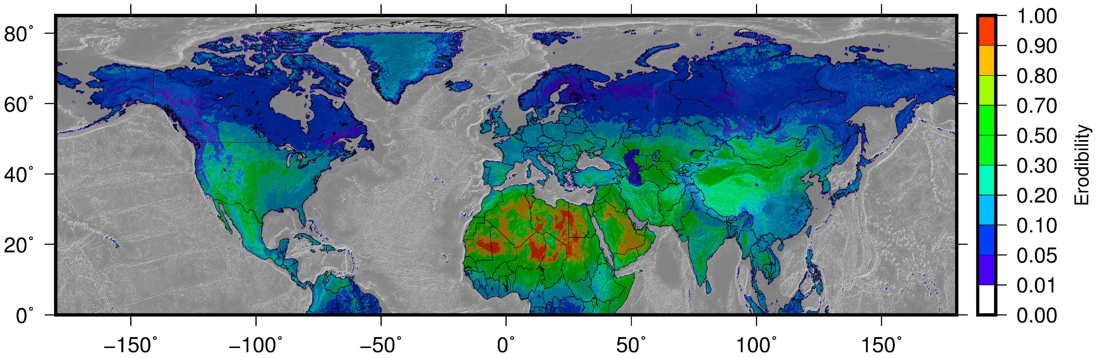
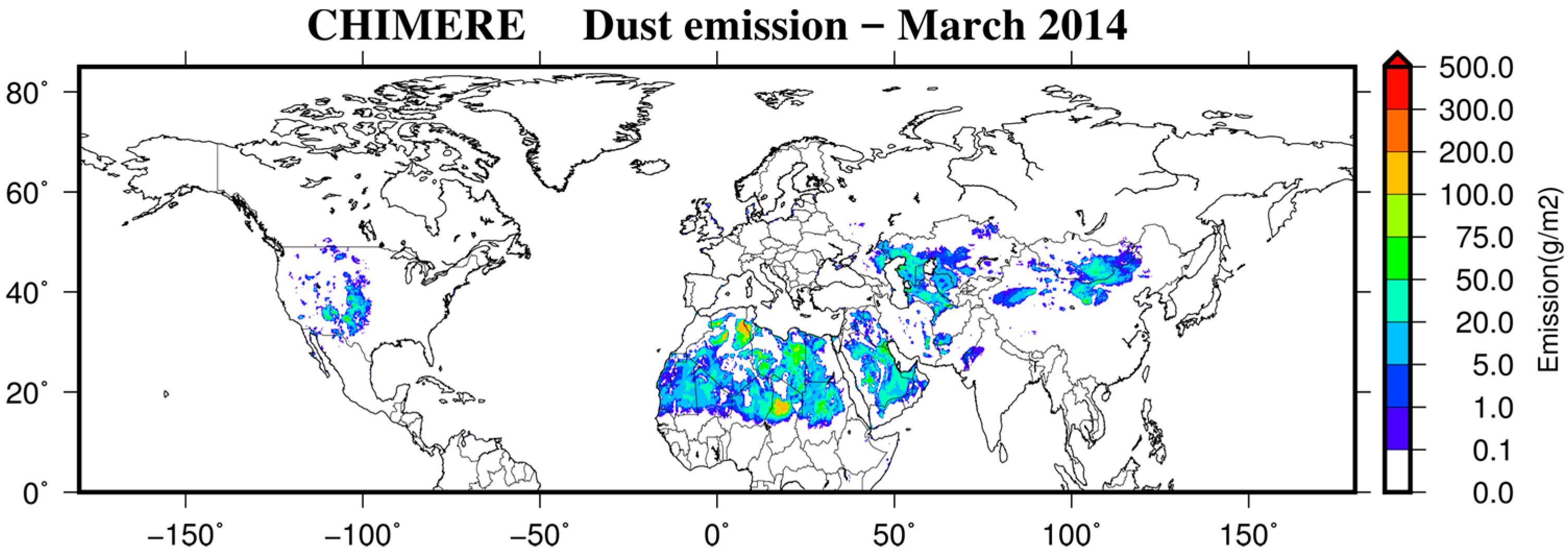
2.2. Dust Emission in CHIMERE

The mineral dust emissions are calculated using the last version of the emission module described in previous studies [46,48,64]. In this model version, the Kok’s [65,66] mineral dust emissions parameterization is proposed, in addition to the schemes described in [67,68]. The vertical dust flux Fd is calculated as described in Equation (1):
F d = C d f b a r e f c l a y ρ a ( u * 2 u * t 2 ) u * s t ( u * u * t ) C α u * s t u * s t 0 u * s t 0 u * s t = u * t ρ a ρ a 0 C d = C d 0 e x p ( C e u * s t u * s t 0 u * s t 0 ) C e = 2.0 ;   C α = 2.7 ;   u * s t 0 = 0.16   m   s 1 ;   ρ a 0 = 1.225   k g   m 3 ; C d 0 = 4.4   × 10 5
where fbare and fclay represent the relative fraction of bare soil and clay soil content, respectively; ρa is the air density; and Cd the coefficient of erodibility. The flux is calculated only if u > u∗t, the threshold friction velocity, u∗t, is calculated using two possible schemes up to the user [69,70]. The corresponding u∗st is this friction velocity but for a standard atmospheric density. The vertical dust flux is integrated over the whole size distribution of particles. The Dust Production Model and its parameters are fully described in [46,71]. To have global and highly spatially resolved surface databases, the module uses the NCAR USGS landuse dataset [72] and the STATSGO-FAO soil dataset [73]. The roughness length is estimated using the global 6 km horizontal resolution “Global Aeolian Roughness Lengths from ASCAT and PARASOL” dataset [74]. The soil erodibility is refined over desert areas using the global erodibility dataset derived from MODIS (Moderate Resolution Imaging Spectroradiometer) data [75], Figure 1 represents the erodibility of soils for the CHIMERE domain, deserts can be clearly identified but large agricultural zones over the US, Europe and Asia are also highlighted in light blue. Some soil and surface parameters are added to limit the emissions fluxes, depending on the period to model and its meteorological conditions. To consider the monthly vegetation variability, the vegetation fraction is diagnosed from the USGS 30s resolution database (from U.S. Geological Survey, accessible at https://landcover.usgs.gov/) and is used as limiter to the erodibility factor. The rain may also inhibit the emission flux and a function is added to stop the fluxes after a precipitation event [46]. The flux may also be limited by the soil humidity and the threshold friction velocity is limited using the Fecan’s scheme [76]. Higher in latitude over Alaska, Canada, Siberia and Greenland, dust emissions can potentially occur [77] due to additional processes specific to or enhanced in cold regions: low temperatures, humidity, strong winds, permafrost and niveo-aeolian processes. Most of these processes are not included in CHIMERE, however for an early spring period such as in this study, the emissions would be turned off due to the snow coverage in these regions.

2.3. Observational Data for the Evaluation of Model Performances

Various sources of data and derived products are used to evaluate the performances of the model for the March 2014 period; they are briefly described below.
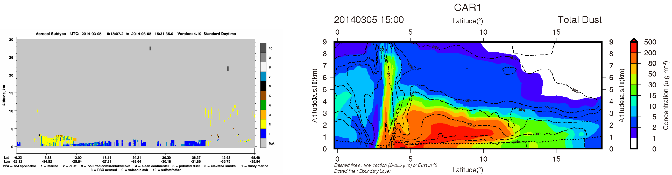
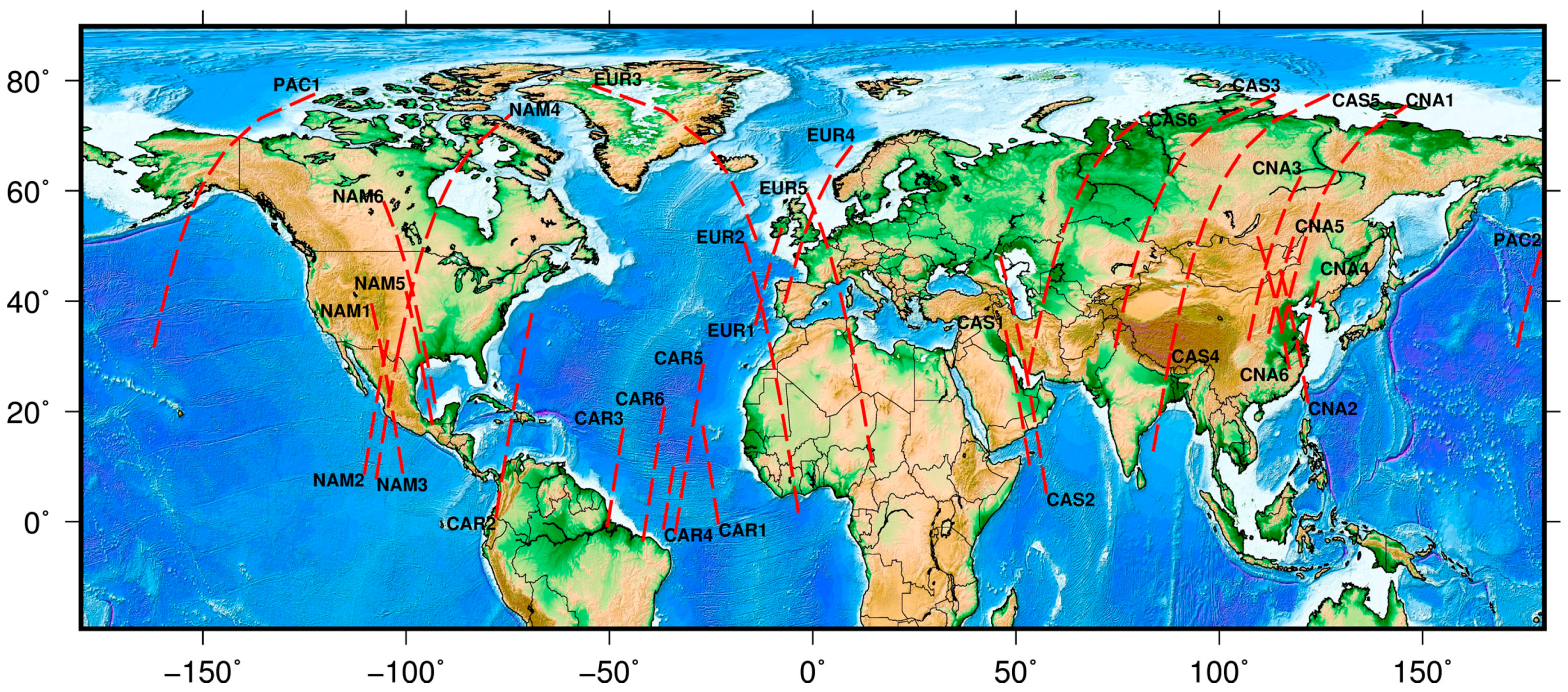
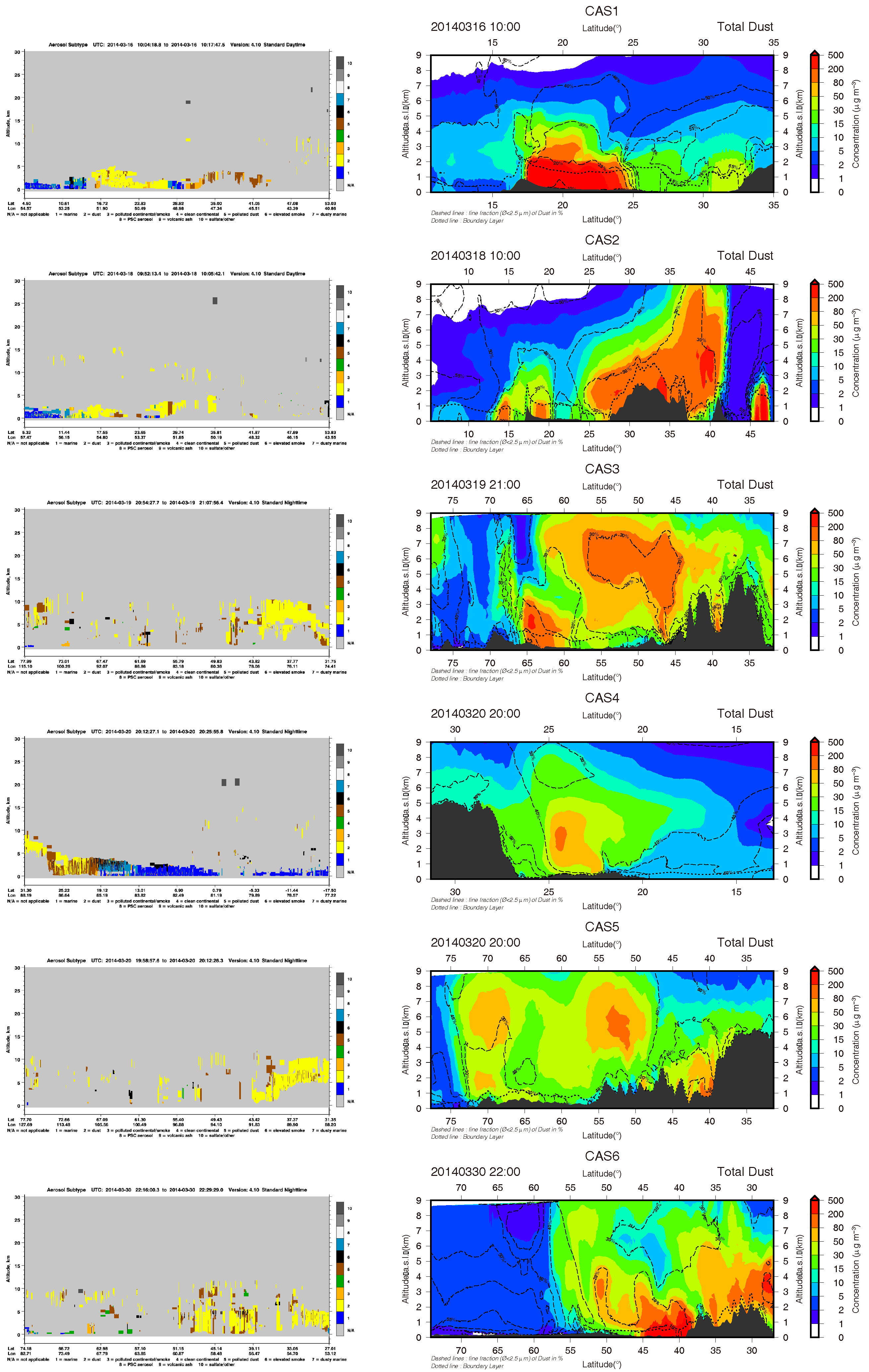
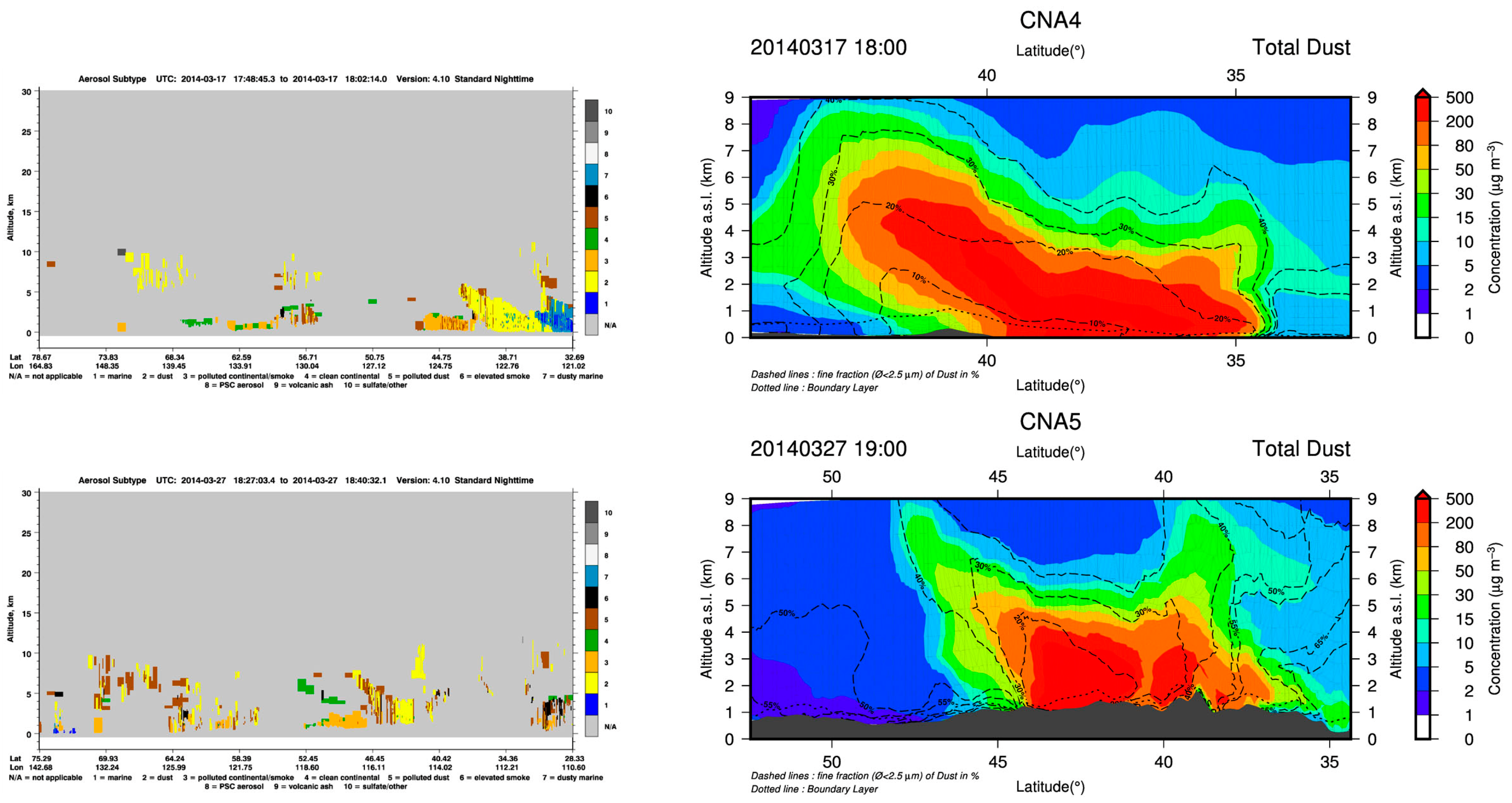
  • CALIPSO and CloudSat, launched in 2006 as part of NASA’s A-train satellite constellation, provide detailed information on cloud and aerosol vertical profiles from tropics to the poles. Cloud vertical profiles are derived from Cloud-Aerosol Lidar with Orthogonal Polarization (CALIOP) [78]. Here, we use the V4.10 dataset [79], cross section of the atmosphere provides various categories separating mineral dust from anthropogenic pollution. The list of selected orbits is given in Figure 2.
  • MODIS (Moderate Resolution Imaging Spectroradiometer) is a key instrument aboard the Terra (originally known as EOS AM-1) and Aqua (originally known as EOS PM-1) satellites. Terra’s orbit around the Earth is timed so that it passes from north to south across the equator in the morning, while Aqua passes south to north over the equator in the afternoon. Terra MODIS and Aqua MODIS are viewing the entire Earth’s surface every 1–2 days, acquiring data in 36 spectral bands, or groups of wavelengths. The MODIS Aerosol Product monitors the ambient aerosol optical thickness over the oceans globally and over the continents. Furthermore, the aerosol size distribution is derived over the oceans, and the aerosol type is derived over the continents. “Fine” aerosols (anthropogenic/pollution) and “course” aerosols (natural particles; e.g., dust) are also derived [80,81]. MODIS products are downloaded from the Worldview tool developed by NASA accessible at https://worldview.earthdata.nasa.gov/. In this paper, the merged Dark Target/Deep Blue Aerosol Optical Depth product will be used. It provides a more global, synoptic view of aerosol optical depth over land and ocean. This layer is created from three algorithms: two “Dark Target” (DT) algorithms for retrieving: (1) over ocean (dark in visible and longer wavelengths); and (2) over vegetated/dark-soiled land (dark in the visible); and the Deep Blue (DB) algorithm, originally developed for retrieving (3) over desert/arid land (bright in the visible wavelengths). Which algorithm is used for a particular location on the Earth depends on its surface cover.
  • The MISR (Multi-angle Imaging SpectroRadiometer) Aerosol Optical Depth Average layer product is also used. This instrument on board Terra displays the temporal averages of all aerosol optical depths calculated from radiances acquired from the green band (555 nm) of MISR’s cameras as an average value for March 2014. This instrument is aboard the Terra satellite.
  • Atmospheric composition data from the US IMPROVE network are also available with PM2.5, PM10 and Soil PM concentrations based on calcium measurements [82]. Daily data are available every three days and available at http://vista.cira.colostate.edu/Improve/improve-data/.
  • Air quality data from the US EPA (Environmental Protection Agency) network provides hourly PM2.5 concentrations accessible at https://www.epa.gov/outdoor-air-quality-data.
  • Data from the Chinese network provides hourly PM10 and PM2.5 concentrations made available for the Beijing area.
  • The French GEOD’AIR database provides PM10 and PM2.5 concentrations for some stations over the French Caribbean Islands in this study (Available online: https://www.geodair.fr/).
  • For the whole Europe, background PM2.5, PM10 and Calcium daily and/or hourly data are retrieved thanks to the EMEP-EBAS database [83]. As a first estimate, Soil PM can be calculated as a first guess from calcium measurements by multiplying the calcium concentrations by a factor of 8 [84].
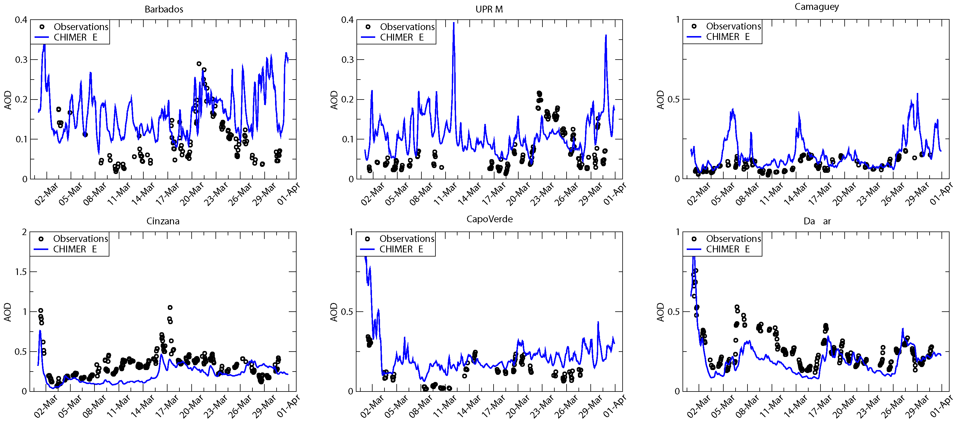
  • The modeled daytime Aerosol Optical Depth (AOD) is compared to observations from the AERONET network [85], available at https://aeronet.gsfc.nasa.gov from the daily AERONET level-2 measurements AERONET-AOD at 870 nm. Unfortunately, AERONET measurements can be used in clear sky conditions areas generally below 20° N in latitude over the Northern Hemisphere, while the model can simulate the AOD for all types of sky. For Europe [86], Central Asia or North America, most dust outbreaks are issued from low-pressure systems and then imply cloudy conditions that makes impossible to use level 2 AERONET products to detect these episodes since most of data are ruled out due to clouds.
  • Synoptic data called SYNOP from the World Meteorological Organization (WMO) provide reporting weather observations made by manned and automated weather stations. The following ten types of coded data have been selected to identify observed dust episodes: “widespread dust in suspension not raised by wind”, “dust or sand raised by wind”, “well developed dust or sand whirls”, “dust or sand storm within sight but not at station”, “slight to moderate dust storm decreasing in intensity”, “slight to moderate dust storm, no change”, “slight to moderate dust storm, increasing in intensity”, “severe dust storm, decreasing in intensity”, “severe dust storm, no change”, and “severe dust storm, increasing in intensity”. The categories “Haze” and “Smoke” have not been considered. These observations remain subjective as they are man-based observations: they can be mixed-up with anthropogenic, wildfires pollution, or misty and foggy conditions, but, in some locations, such as in Central Asia, this information is the only one we can access.
  • Additional data from isolated stations or issued from previous publications will be used to assess the model performances.
Maps of site locations of interest and discussed in this study are provided in Figure S6 in the Supplementary Materials.

3. Discussion Results at the Hemispheric Scale

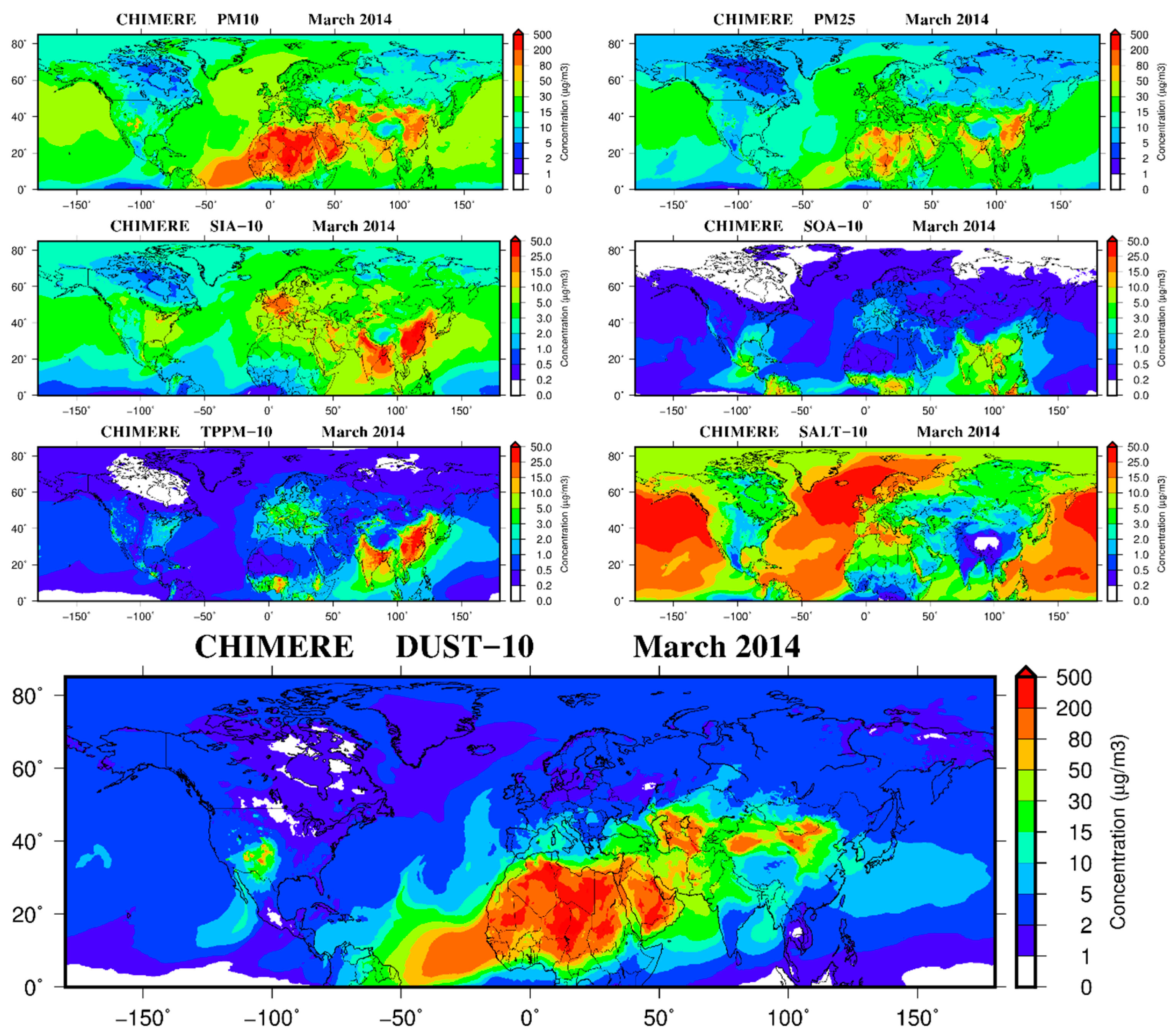
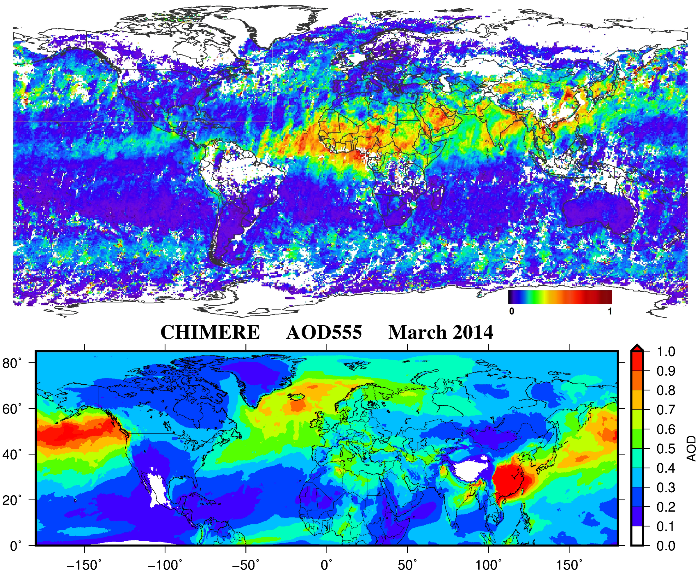
3.1. Overview of PM Concentrations Simulated by CHIMERE over the Northern Hemisphere in March 2014

The map of total emissions for March 2014 is displayed in Figure 3. This map is a combination of the various meteorological and soils related processes computed on an hourly basis. The main emission areas are closely linked to the erodibility map (Figure 1), the main desert area can be clearly identified (Algeria, Tunisia, Libya, Gobi Desert in China and Mongolia, Arabian Peninsula and to a lesser extent the US desert area) and particularly the Bodélé depression in the south of the Sahara (Chad) which is the most intense source of dust worldwide. In Europe, and especially in Spain, the too high soil moistures in this season makes impossible the emission of agricultural dust. Significant dust emissions around the Caspian Sea are simulated; this specific pattern is discussed in Section 4.4.
Figure 4 represents the mean surface concentration maps of PM for March 2014 over the Northern Hemisphere. The main hot spots of PM10 concentrations are located over the arid and semi-arid regions and also over the most populated areas in Asia. High PM levels are simulated in the southwest of the USA. For the SIA species, the patterns are rather different with high concentrations observed in Europe dominated by ammonium nitrate concentrations and in Asia with mainly due to sulfate. The influence of PM pollution events [87] is very strong and usual for the early spring period. In March, high SOA concentrations are simulated below the 40° N latitude, the contribution of biogenic species is important in Africa and South America while the contribution of anthropogenic emissions is more important in Asia. The primary emissions are very large over the most populated areas in Asia and Africa (e.g., Nigeria). Sea salt emissions are mostly influenced by wind speed and the resulting concentrations are obviously high over the North Pacific and Atlantic oceans where the low-pressure systems are still active in early spring, the order of magnitude is in agreement with observational data as reported on coastal areas [88,89].
At the global scale, the PM pattern is largely influenced by the dust concentrations, two dust plumes issued from the continental areas can be observed from the Southwest US to the South Pacific and from the Sahara to the Caribbean area. A more diluted transport of dust is also observed over the North Pacific Ocean. For mineral dust, the comparison with observational data is difficult, as such data are very scarce in the literature. Globally, the patterns of surface dust concentrations in the bottom panel of Figure 4 are very close to the multiannual structure shown in previous studies based on SYNOP meteorological observations [90], moreover the global increase of dust load in Figures S7–S10 in Supplementary Materials during the course of March 2014 is confirmed by data reported in previous works showing the yearly cycle of dust concentrations with the beginning of the “dust season” in February over the Northern Hemisphere [91].
Observational data for a March period based on available data are reported in the literature [92], unfortunately the exact data are not available: observed values are averaged from available data, but a first estimate shows that CHIMERE for March 2014 produces the same order of magnitude for dust concentrations, the main hot spots in Cape Verde (16.70° N–22.90° W) and Izaña (28.30° N–16.50° W) are rather well reproduced by the models with respectively about 100 and 10 µg m−3 against observed values generally close to 200 and 30 µg m−3. Better agreements are found over two islands in front of China coasts with for instance in Cheju (33.52° N–126.48° E) about 27 µg m−3 for the measurements and 20 µg m−3 predicted by CHIMERE.
The lowest values (<1 µg m−3) of surface dust concentrations are simulated over the Equatorial Pacific, this is certainly due to low dust emissions downwind to the prevailing air mass fluxes from Central and South America. From Central to North Pacific the mean surface concentrations lie in the range 2–10 µg m−3 that are usual for a March period which generally exhibits the highest dust concentrations over the Pacific Ocean [91], these orders of magnitude are fully in line with the SEAREX experiments findings [93]. In Alaska, the CHIMERE model exhibits dust concentrations in the fine mode of particles 5 to 10 times overestimated at IMPROVE Stations (Denali 63.72° N–148.97° W, Gates of the Arctic 66.90° N–151.52° W and Trapper Creek 62.31° N–150.32° W) with observational data usually in the range 0.01–0.4 µg m−3 while CHIMERE simulates concentrations up to 1 to 5 µg m−3, however the end of March 2014 increase of concentrations is well reproduced by the model. This overestimation of background concentrations over remote areas is shared by several global models participating to the AeroCom phase I project [94], and also identified in the Conformal Cubic Atmospheric Model (CCAM) [95] where the dust lifetime is longer than the ones calculated in previous modeling exercises.
Even if the objective of the paper is not to perform an exhaustive evaluation of the model for criteria pollutants, as it has been made in past studies (see previous sections for adequate references), Table 1 presents an overview of the model performances for PM2.5 over Beijing, Europe and the USA. The performances will be more detailed in the next sections to analyze the ability of the model to simulate the identified dust events. For Beijing, the daily correlation is very good and the bias very low for this period. For Europe, as is generally the case in this period, an underestimation of PM2.5 concentrations is observed but the correlation is rather good, particularly the spatial correlation. This underestimation is due to underpredicted ammonium nitrate concentrations in early spring pollution events and a lack of wood burning emissions (from the residential sector) in emission inventories [54]. For the USA, a negative bias is also observed with a lower correlation mainly driven by a low spatial correlation. In addition, Table S1 in Supplementary Materials provides an overview of the evaluation at AERONET sites; at these sites, CHIMERE generally overestimates the AOD and the time correlation is poor, except at low latitude stations where more hourly data are available thanks to clear sky conditions. However, the spatial correlation is better.

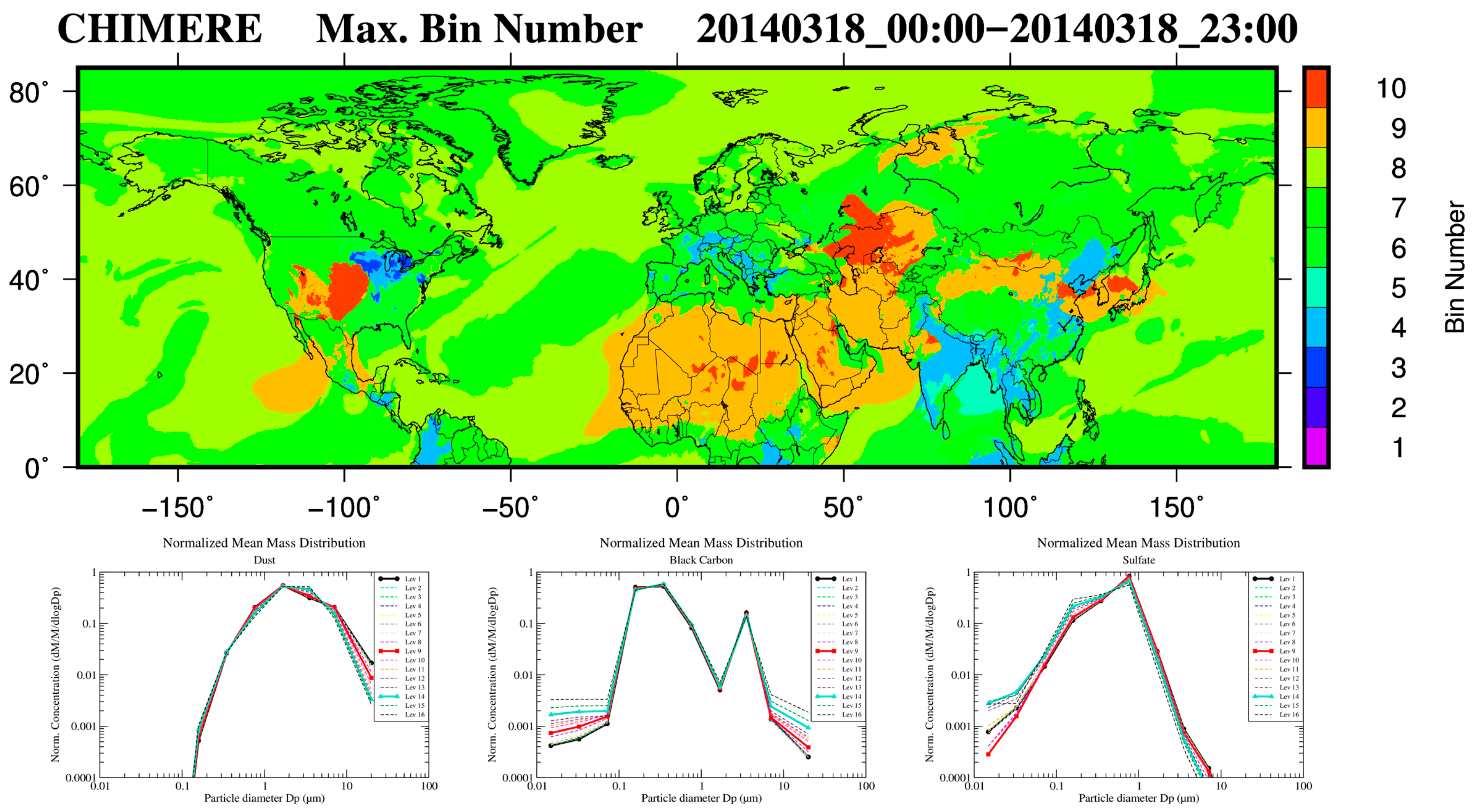
3.2. Particle Size Distribution

The period 16–19 March is very active for dust episodes at the global scale; several outbreaks of dust in Asia and USA are observed occurring at the same time (Figure 5). These events will be discussed later in the regional focus of the study. The dust transport in Asia can be observed with pollution plumes advected toward the Pacific Ocean later in March, a transatlantic transport of dust from Africa to the Caribbean is also simulated on 16 March. Over North America, dust from the southwest of USA are transported over the Pacific Ocean. For this date, the bin number providing the maximum PM concentration is also plotted (Figure 6). This maximum is the highest close to the dust emissions area with a peak around bin 9 and 10, i.e., around 10 µm. This peak is below 2.5 µm (bin 5 and 6) for areas influenced by anthropogenic sources, and in-between elsewhere. At the bottom of Figure 6, the mean normalized size distributions for dust is displayed and compared to black carbon and sulfate species. This distribution is averaged over the whole hemispheric domain for each 16 model levels from the surface to the top on 18 March 2014. On average, for dust, a single peak around 2 µm in particle diameter is predicted by the model, the contribution of the last bin decreases for the highest levels consistent with the effect of particles sedimentation, however a slight shift of the accumulation mode toward the coarse particles is also simulated as a consequence of particle growing by condensation of secondary species. The black carbon distribution displays a bi-modal pattern around 0.2 µm and 3 µm and consistent to what was observed in Europe during field campaigns on background sites [96]. For sulfates, the model simulates a single distribution peak around 0.8 µm and also high concentrations around 0.2 µm; this is consistent with experimental findings [97,98] as the results of condensation of sulfate on the maximum of available particle surface for mass transfer. For AERONET sites, a main mode is generally observed around 4 µm and a second peak around 0.2 µm [99], this second peak being certainly due to anthropogenic sources (since the measurement is performed within the city), the main peak being driven by windblown dust emissions. In CHIMERE, internal mixing is assumed for aerosol particles; therefore, mineral dust participates directly or indirectly to chemical and microphysical processes (coagulation, condensation so far). This assumption is validated by experimental evidences in many studies [100] and allows a full interaction between all constitutive species of particles. Nevertheless, in this version of CHIMERE the formation of coarse nitrate due to the reaction of calcium with nitric acid (issued from the anthropogenic pollution) is not considered and could enhance the interactions between natural and anthropogenic emissions as it has been studied in China [101].
The transport of “giant” mineral particles, which can be defined as particles with diameters exceeding 10 µm, is rarely documented in the literature according to a recent study [102]. This study analyzes a specific Asian episode leading to the delivery of big particles in Korea thanks to mid-tropospheric strong winds. In Figure 6, the pattern close to Korea (showing that the maximum size bin is largely influenced by dust) confirms the possibility of long-range transport of “giant” particles far from emission areas. As mentioned in the Introduction, the added value of using models with fine horizontal resolutions [33] allows to better reproduce the processes of particle lifting like through the parametrization of deep convection processes activated in this version of CHIMERE [48]. However as suggested in [33], an explicit resolution of convection will enhance the capacity of the model to transport big particles on very long-range transport, but this remains too much time consuming so far for such large domains. Moreover, a recent study describing a conceptual model of dust dynamics showed that vertical transport can efficiently counteracts and limits the gravitational settling of coarse particles [103], according to Lidar observations in the frame of the SALTRACE experiment.
The evolution of the particle sizes is also shown in Figure 7 which provides an overview of dust concentration fields through latitudinal cross sections [0° N–90° N] averaged over boxes encompassing the Pacific and Atlantic Oceans, respectively, within longitudes ranges of [122° E–124° W] and [80° W–17° W]. Over the Pacific Ocean, concentrations peaks are located at 2–3 km in altitude at the interface with the boundary layer in mid latitude regions 35–40° N resulting mainly of the trans-Pacific transport of Asian dust emissions mixed with diluted Saharan dust transported by southwesterly fluxes. In Figure 7, the deep convection updraft flux integrated over the column is displayed as an indicator of the convective activity. A peak is observed over the Equatorial Pacific and an increase is also observed at mid latitudes, these convective processes could enhance the lift of dust particles within the free troposphere. Over the Atlantic Ocean the altitude of the maximum dust concentrations is lower, located within the marine boundary layer and very close to the Equatorial area at 5–10° N as the results of trans-Atlantic transport of Saharan dust by the trade winds (easterly flux). The dust concentrations peak are linked to the lowest contributions of fine particles (with diameter lower than 2.5 µm), in background areas of the atmosphere the fine fraction contribution is generally higher due to the sedimentation and dry deposition of the biggest particles. In the lower troposphere, the lowest concentrations are simulated near the polar easterlies area (about 60° N) with a second concentrations peak between 2 and 3 km in altitude in the polar cell above 80° N; this specific location over the poles is confirmed during the AeroCom experiment [104]. A close look at vertical wind speeds shows slight positive vertical winds around 2–3 km in altitude (Figure S11 in Supplementary Materials) upper in altitude, which can explain this feature, generating stagnant conditions leading to higher concentrations. However, a slight increase of ground wind speed is observed, indeed if wind velocities are generally low in this region, sudden gales can be frequently observed then affecting the averaged monthly values.

3.3. Deposition of Mineral Dust in March 2014

Dust deposition fluxes are larger over the Atlantic Ocean compared to the Pacific Ocean due to higher concentrations over the Atlantic, except over mid latitude over Pacific between 30 and 50° N. On the Northern Hemisphere, the dry deposition simulated by CHIMERE dominates the total deposition (Figure S11 in Supplementary Materials), while global models generally overestimate the role of wet deposition as described in [94]. The total monthly averaged deposition fluxes (wet and dry) are in line with those reported in the literature [105] presented on a yearly basis even if the range of model results can vary within an order of magnitude due to differences in dust emissions and the parameterization of processes. A ratio Ω for the dry (d) and wet (w) deposition processes at a given latitude (lat) defined in the set of Equation (2), as the ratio of scavenging coefficients in the coarse (defined here as particle diameter in the range 2.5–40 µm) over scavenging coefficient in the fine fraction of dust (particle diameter below 2.5 µm):
C mode col , lat ( day ) ¯ = ver = 1 H top lon = 1 Nlon hour = 1 24 C mode ( hour , lon , lat , ver ) × Δ H ( ver ) H top × Nlon × 24 C mode ground , lat ( day ) ¯ = lon = 1 Nlon hour = 1 24 C mode ( hour , lon , lat , 1 ) Nlon × 24 mode = fine ( φ < 2.5   μ m )   or   coarse ( 2.5   μ m < φ < 20   μ m ) D dep , mode , lat ( day ) ¯ = lon = 1 Nlon hour = 1 24 D dep , mode ( hour , lon ) Nlon × 24 dep = w   or   d   ( respectively   for   wet   or   dry   deposition ) Λ w ,   mode lat ( day ) = D w , mode , lat ( day ) ¯ C mode col , lat ( day ) ¯    Λ d ,   mode lat ( day ) = D d , mode , lat ( day ) ¯ C mode ground , lat ( day ) ¯ Ω w lat = Λ w , coarse lat ( day ) ¯ Λ w , fine lat ( day )   if ( Λ w , fine lat ( day ) 0 ) Ω d lat = Λ d , coarse lat ( day ) ¯ Λ d , fine lat ( day )   if ( Λ d , fine lat ( day ) 0 )
where D (µg cm−2 s−1) and C (µg cm−3) are, respectively, the deposition fluxes (dry or wet) and concentrations for dust in the coarse and fine fraction of particles averaged over hours, longitude (lon); and Nlon is the number of longitudes considered. The concentrations are vertically averaged (ver = 1–16, Htop is the top of the vertical mesh) for the wet deposition as it concerns the whole column (col) by in- and sub-cloud scavenging, and for dry deposition only the ground concentration is used. The scavenging coefficient Λ is a type of daily deposition velocities for a given latitude for the coarse and fine fractions of dust expressed in m s−1. An increase of the fine fraction of dust is modeled in the equatorial area particularly over the Atlantic Ocean with an increase of the altitude of the maximum concentrations certainly in relation to an increase of the magnitude of precipitations (Figure 7), which are peaking during this season in equatorial areas. Indeed, precipitations remove the biggest particles by impaction processes by sub-cloud scavenging while the smallest ones will be less influenced [104] except by Brownian motions, this behavior observed over the Atlantic Ocean at 0–5° N close to the equator is consistent with the patterns for the Pacific Ocean with a slight shift towards northern latitudes (about 10° N). This behavior is highlighted in Figure 7 with an increase of the Ωw ratio for wet deposition close to the equator in relation with an increase of precipitations. Moreover, Ωw is anti-correlated with the cloud water content: when this parameter increases the in-cloud scavenging increases leading to lower differences (decrease of Ω) between the washout of the coarse and fine fractions of dust because there are no differences between the treatment of in-cloud scavenging for coarse and fine particles in CHIMERE [46]. However, this ratio Ωw is generally high with values above 10 and even 200 close to the equator meaning that sub-cloud scavenging largely dominates the dust deposition in this area. These Ωw large values are the results of a sharp increase of the impact efficiency between falling droplets and the particles with diameters between 2 and 10 µm, which can change with two orders of magnitude [106,107]. Over the northern latitudes (above 70° N), particularly over the Pacific Ocean, the precipitation decreases, the dry deposition fluxes become higher than the wet deposition, the wind speed increases and governs the dry deposition fluxes that is known to be positively correlated with wind velocity [108]. On average, Ωd is in the range 3–10, meaning that coarse particles are more influenced by dry deposition due to higher sedimentation velocities.

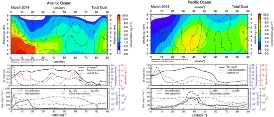
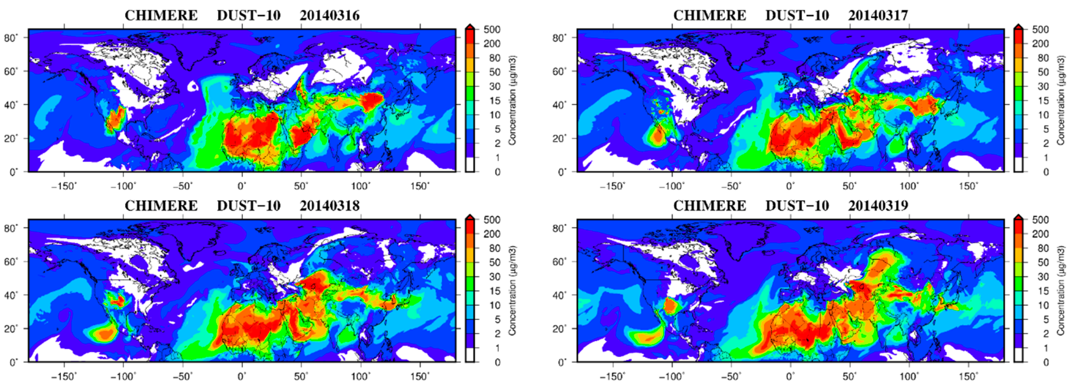
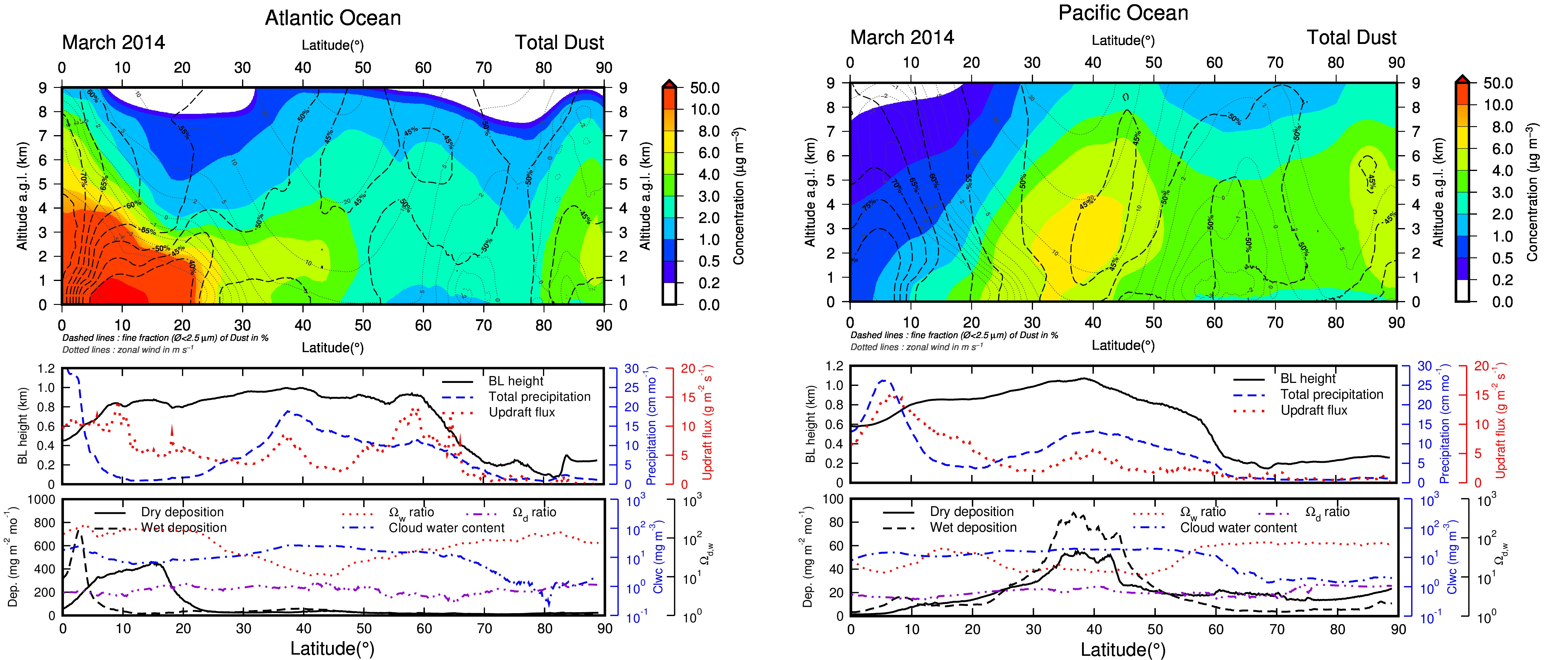
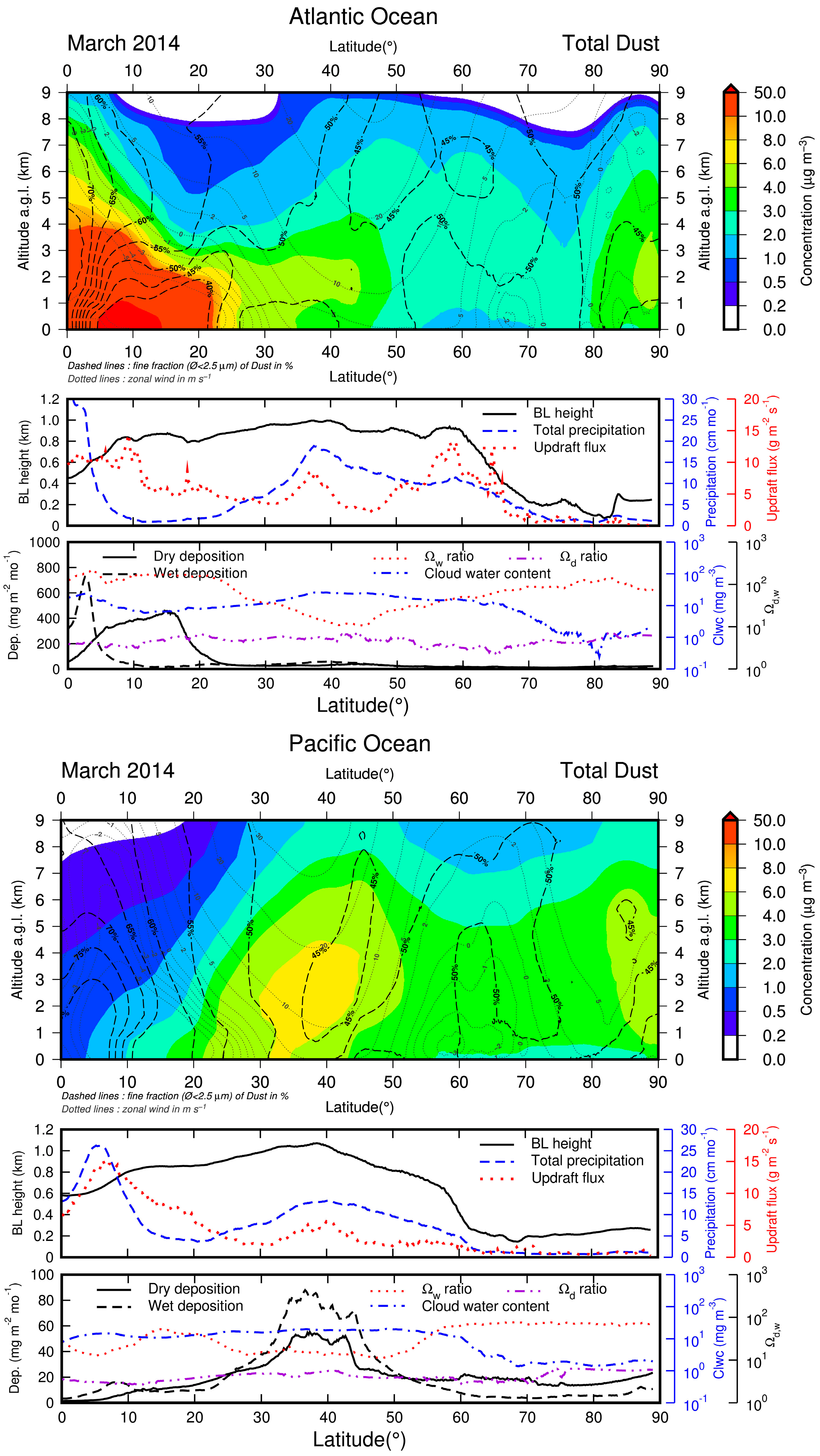
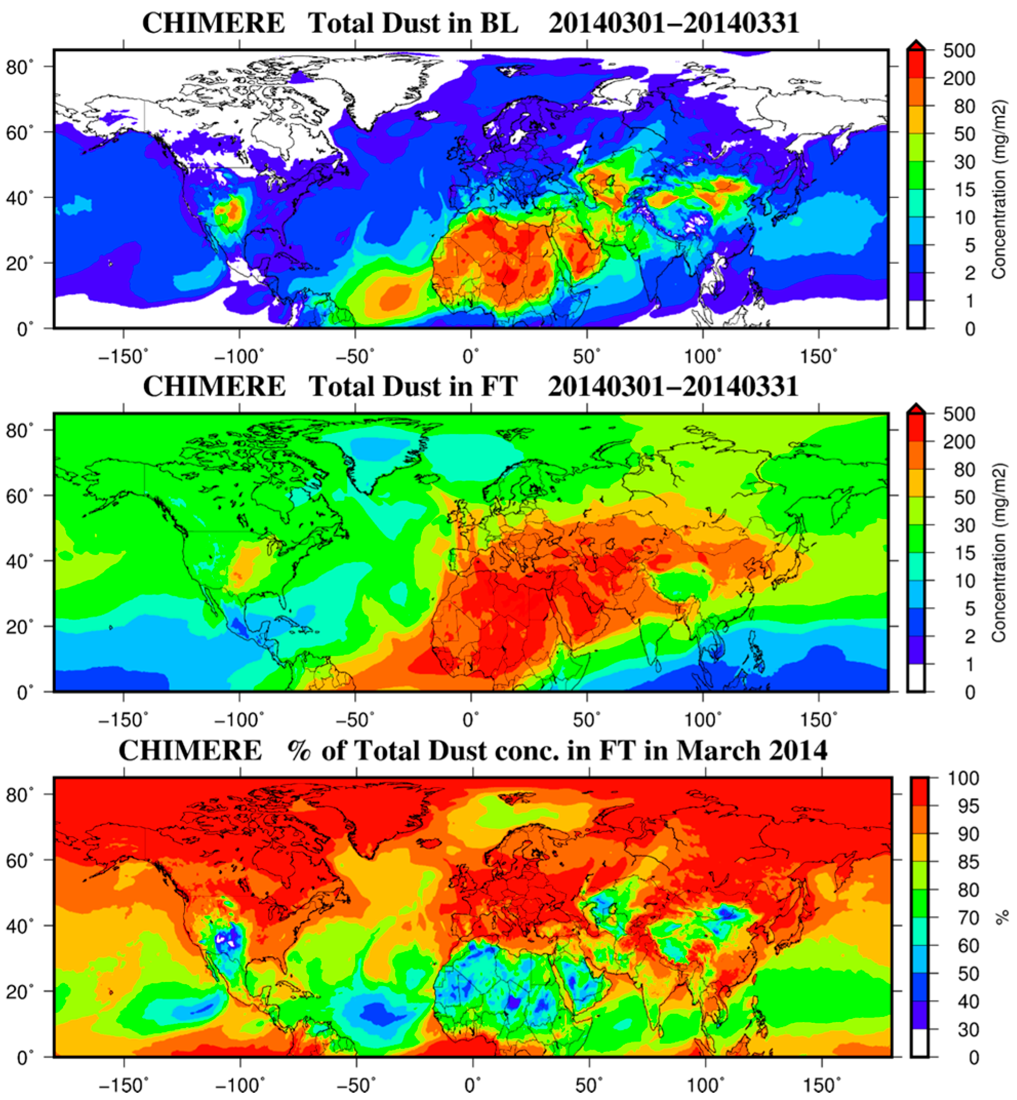
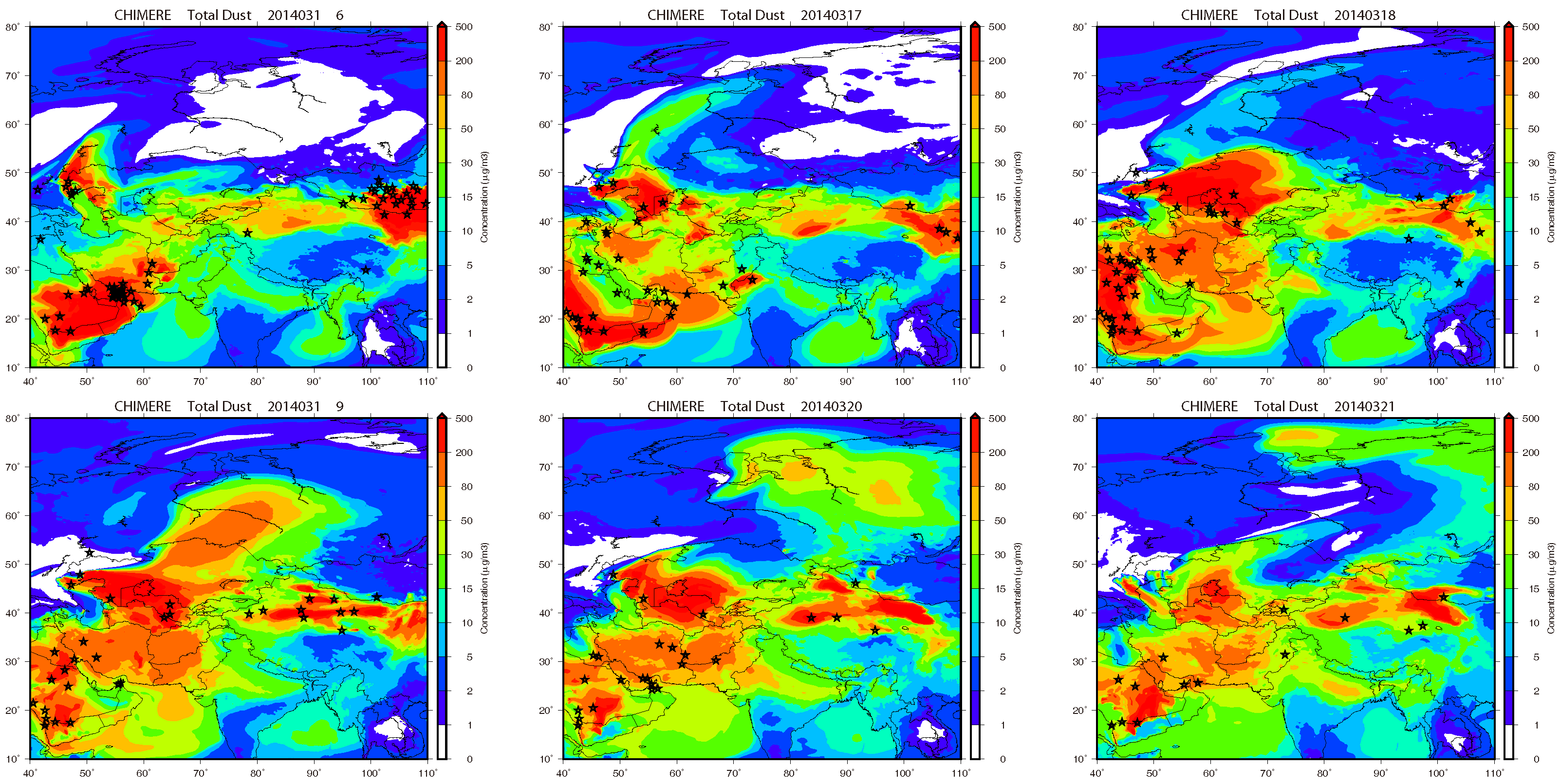
3.4. Transport of Mineral Dust Simulated by CHIMERE in March 2014

Figure 8 shows the monthly averaged integrated dust concentrations C (in mg m−2) over the boundary layer (BL) as provided by the meteorological driver and the free troposphere (FT) height according Equation (3), the ratio of the FT concentrations to the total column (BL + FT) is also represented as computed in Equation (4). ∆h is the thickness of CHIMERE layers, and a minimum of BL is used as the first CHIMERE layer (about 30 m).
C B L   o r   F T [ mg   m 2 ] = h = B L   o r   F T ( t i m e   C [ µ g   m 3 ] × Δ h [ m ] / 1000 )
R a t i o   ( % ) = C F T [ mg   m 2 ] / ( C F T [ mg   m 2 ] + C B L [ mg   m 2 ] )
Figure 8 reveals the transport of dust over the Northern Hemisphere. Figures S7–S10 in Supplementary Materials provide the full daily evolution of the concentrations in March 2014. A more spread structure in the FT is observed with a shift towards the northeast compared to the concentrations within the BL. Generally, the highest dust loads are located and diluted in the FT allowing an efficient long-range transport as they are less influenced by deposition and submitted to high velocity winds. Above the 45° N latitude, more than 80% of the dust load is in the free troposphere. Around the 40° N latitude areas, the transpacific transport of dust from Asia to the USA used the free troposphere routes while this transport seems more balanced between Africa and the Caribbean area. High dust loads in the BL are simulated over the emission source areas partly because of elevated height of BL in these regions. Western Europe is clearly affected by dust transport in the FT. In Figures S7–S10 in Supplementary Material, we can clearly see the evolution of the dust emitted in Africa and the Middle East at the beginning of March, and blown up into the FT and transported over East Asia during mid-March. At the end of March, a large plume emitted in Africa flies over Europe and reaches the Arctic, participating to the accumulation of dust in this region as previously described.
An overview of the aerosol load can be observed from space using the equipment on board Terra and Aqua satellites. The MIRS instrument as previously described allows to generate monthly maps of AOD at 555 nm such as the one presented in Figure 9 (top panel). Unfortunately, the cloud screening does not allow a full overview of the aerosol load across the world particularly at the highest latitudes (where a lack of sunlight at certain time of year is also responsible for a poor retrieval at the highest latitudes). In the bottom panel of Figure 9, the AOD computed by CHIMERE provides the AOD 555 nm without cloud screening. The model underestimates the AOD in the lowest latitude mainly due to the missing fire emissions that are not included in this simulation, however the pattern of dust from Africa to the Caribbean zone can be identified. Over the North Atlantic and Pacific Ocean, the high AOD simulated is mainly due to sea salts over the Atlantic Ocean (due to a high absorption of water by sea salts in ISORROPIA calculations) and a mix with anthropogenic aerosols and natural dust over the Pacific Ocean; this pattern can be observed by the MISR instrument but with a lower intensity due to the cloud screening. Elsewhere at lower latitude, in India for instance, as March is a month with clear sky conditions (pre-monsoon season in many regions), a comparison between CHIMERE and MISR data can be performed and, generally, the same pattern can be observed with an underestimation of CHIMERE AOD. The Chinese plume simulated by CHIMERE cannot be caught by the instrument due to the presence of clouds but a small fraction can be observed over the Beijing area.

4. Discussion on Regional Dust Events

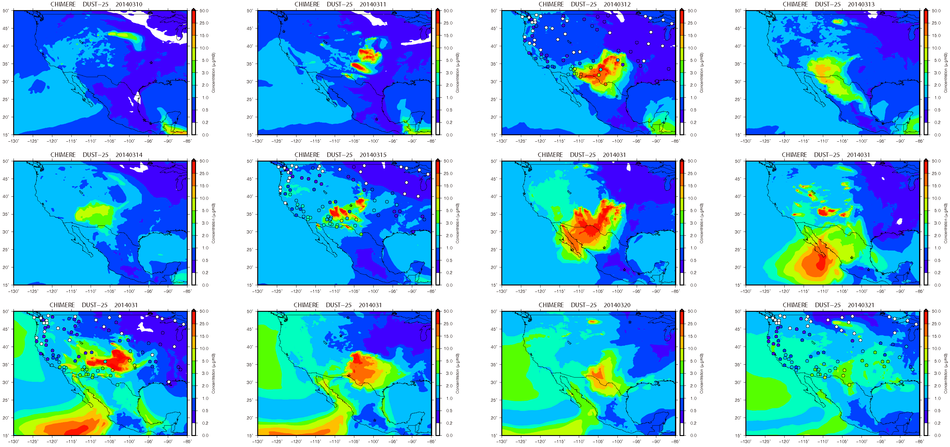
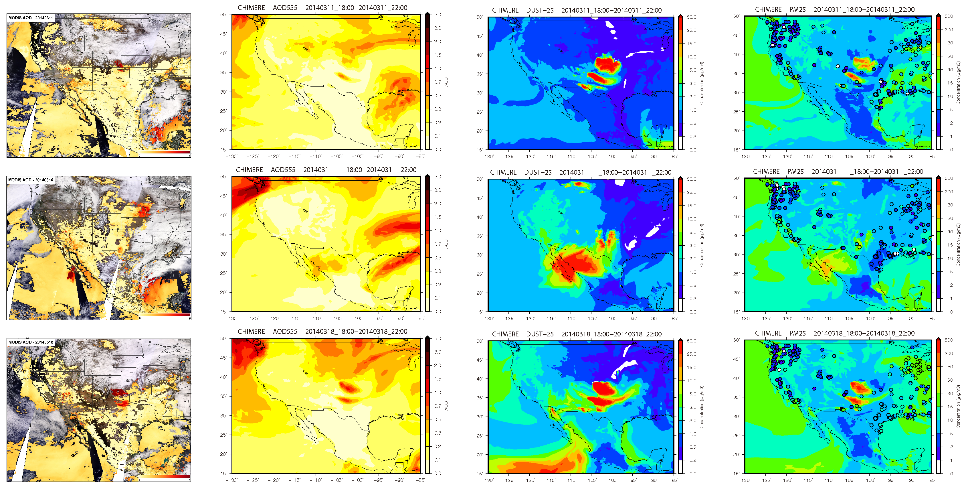
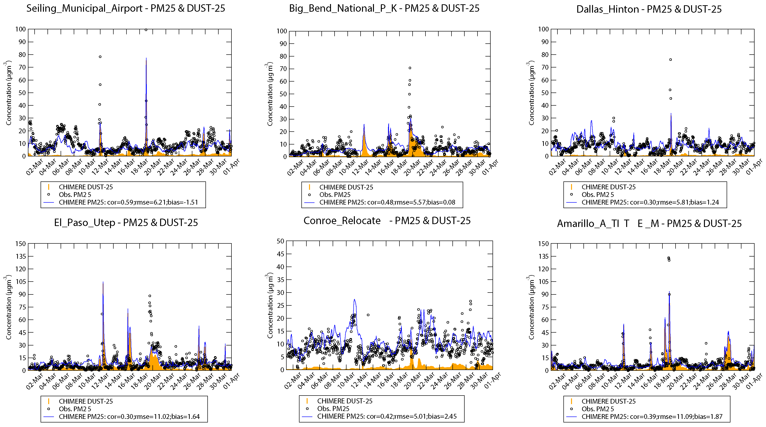
4.1. Dust Outbreaks over North America

In arid and semi-arid climates of North America (Arizona, New Mexico, California, Utah, Colorado and Texas), dust storms are commonly observed, particularly during the March–May period [109,110]. Several dust episodes can be observed over the southern USA in March 2014, some of them have been discussed and commented in media and press release of scientific institutions only. Over North America, on 11–12, 16, and 18–19 March, episodes were reported in media [111] and institutional Internet resources [112,113]. The 18 March episode was particularly commented: a low-pressure system brought strong winds—gusting to 85 km h−1—to the Southern Plains. The winds picked up exposed soil from the parched landscape, resulting in a large dust storm that covered parts of Colorado, Kansas, Oklahoma, New Mexico, and Texas. The storm was the second in the week to sweep across the region with similar wind patterns. The dust originated from New Mexico. The plume stretched across about 175 km, but was dissipated a couple of hours later. The large images reported in the NASA report [113] shows dust across a wider area, including a second large dust plume in southern Colorado, Kansas, and Oklahoma.
Some stations from the USEPA air quality network have been selected to analyze the March 2014 dust events close to soil dust emission areas, mostly in the southwest of US (Figure 10). PM2.5 observations have been selected to be consistent with the IMPROVE data mainly focused in fine fraction of particles. The three episodes can be identified in most of selected stations and are clearly correlated to the presence of dust in the model outputs. The correlation coefficient based on hourly values is in the range 0.3 to 0.6 at these stations and the timing of the soil dust episodes is rather good (a correlation based on hourly value is very hard for such a model), however the intensity of these events is underestimated at the station. On average, the bias is rather low, the background observed and simulated concentrations are closed to 10 µg m−3. During the dust outbreaks, PM2.5 concentrations can reach and exceed 100 µg m−3. The evolution of soil dust concentrations in the PM2.5 matrix of particles is displayed in Figure 11 at IMPROVE stations and confirms the ability of the model to rather well locate the pattern of the plume events with sometimes a clear overestimation of dust concentrations during the dust events. However, on average, for IMPROVE stations a negative bias is observed for March 2014, −23%, and a correlation of 0.39. From 16 March, the dust plume is advected toward Mexico over the Baja California region. Manned SYNOP observations indicate the presence of dust from 16 to 21 March particularly in Baja California (Ciudad Constitucion: 25.00° N–111.67° W) where the presence of dust is reported several times on 16 March. All stations in Chihuahua (city located in the very north of Mexico close to the USA border) displays high PM concentrations on 13 March with PM2.5 hourly values largely exceeding 100 µg m−3 at the Sur station (urban station located 28.63° N–106.04° W) and two other peaks on 17 and 21 March; these three events are well detected by CHIMERE despite an underestimation (Figure S12 in Supplementary Materials) certainly due to local dust or resuspension of road traffic dust. Mexican data can be accessed at http://sinaica.inecc.gob.mx/ that is the Air quality information system in Mexico. High concentrations are also observed at this station on 19 and 20 March confirming the extension of the plume far from the emission areas in US. The comparison of CALIPSO data identified as “dusty marine” in Figure S1 in Supplementary Materials (NAM5 trajectory) clearly confirms the dust load within the boundary layer simulated by CHIMERE over the Pacific Ocean between 10° and 30° N, dust is mixed with sea salts (“dusty marine” category for CALIPSO products).
The three events can also be observed thanks to the MODIS data despite the presence of clouds that limits the detection of the full emission areas. As depicted in Figure 12, MODIS data are compared with the AOD computed with CHIMERE at the same wavelength (555 nm), the pattern of over the emission areas in the southeast of Colorado on 11 March and two high concentrations area on 18 March over an area located in the intersection of Colorado, New Mexico and Kansas states and the other one over Texas. On 16 March, the pattern observed by MODIS is more difficult to reproduce, nevertheless the small structure over Texas also exists in the model outputs with a lower intensity, which is confirmed by the PM2.5 observations in this region matching the predicted concentrations.

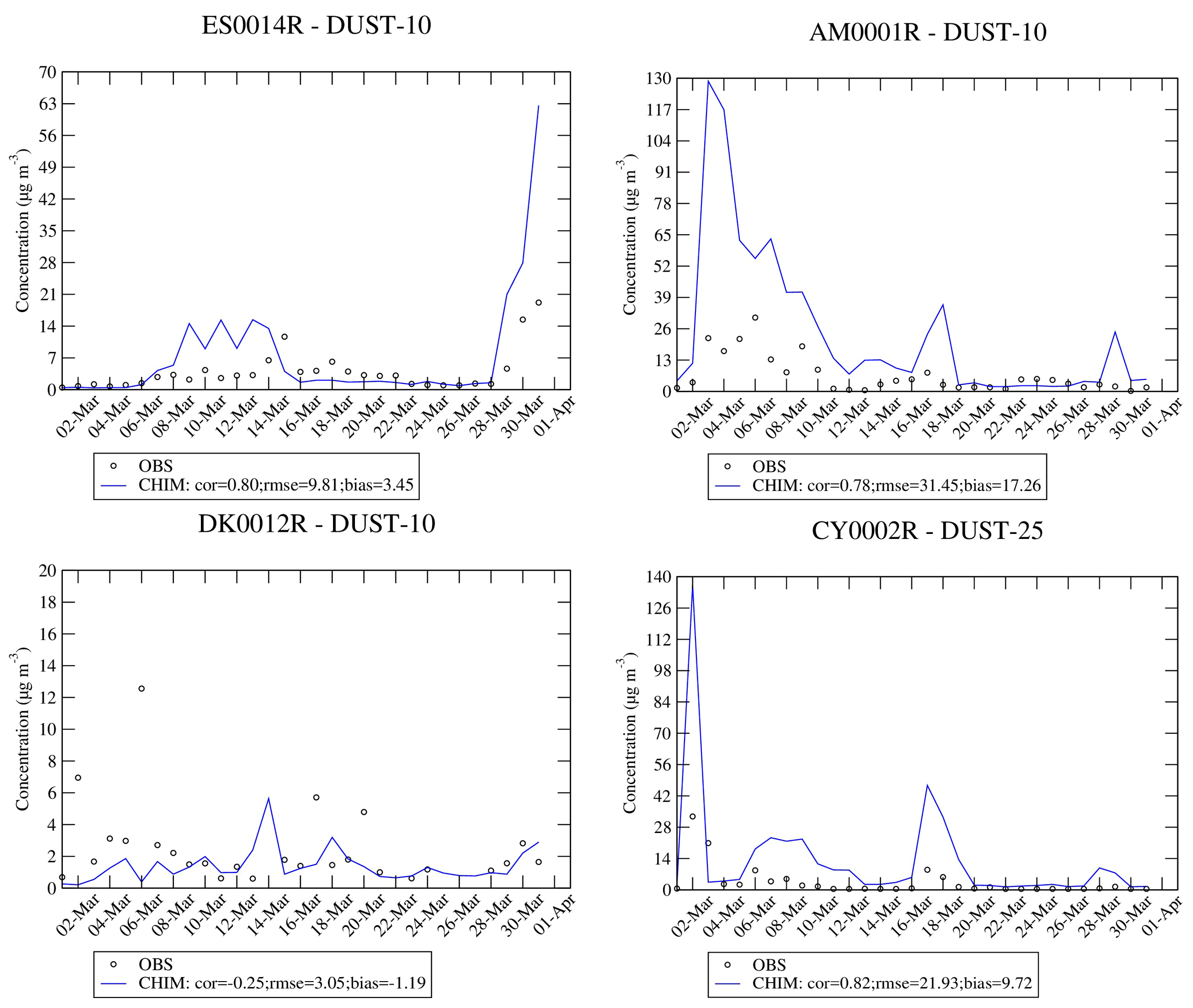
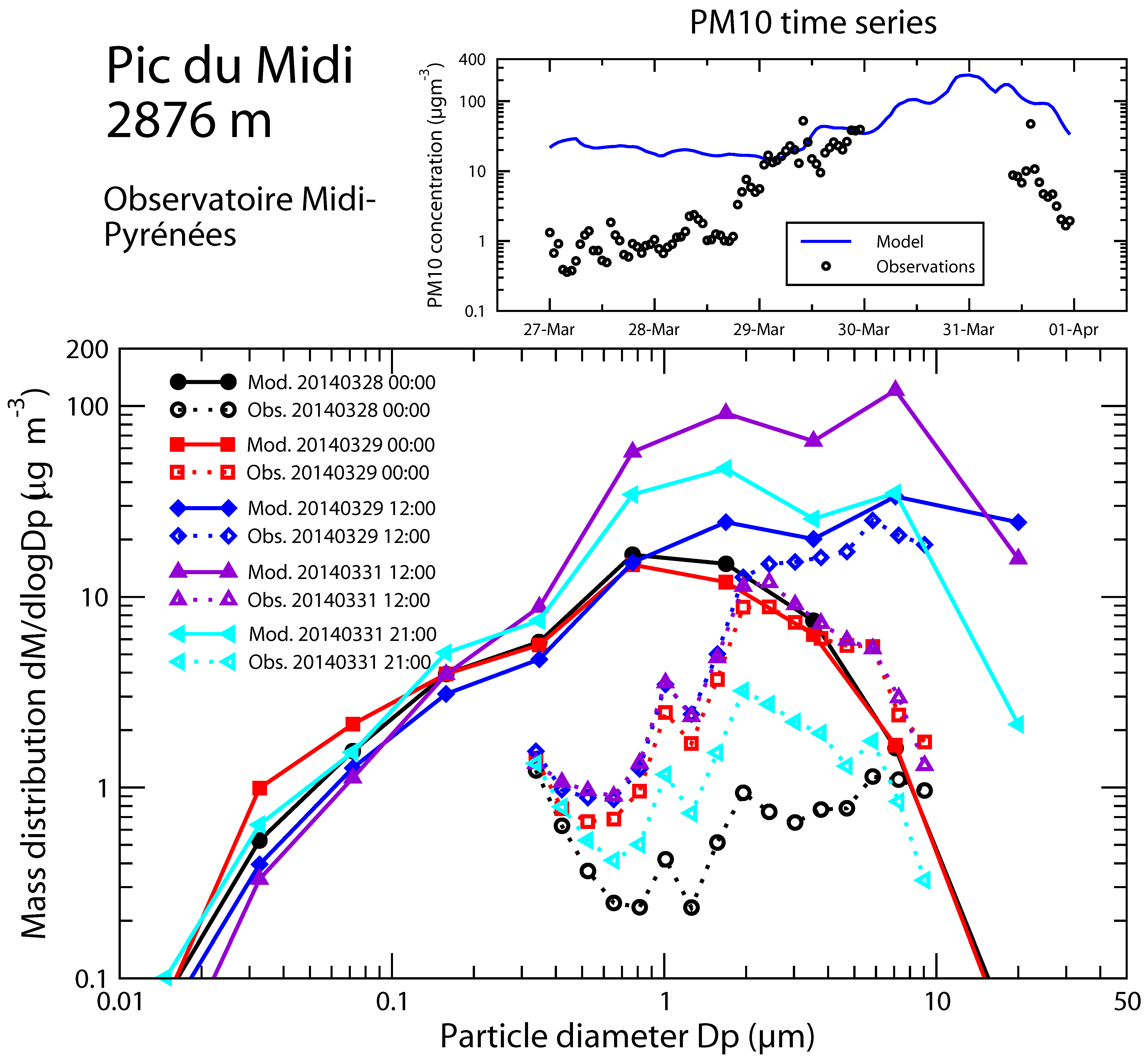
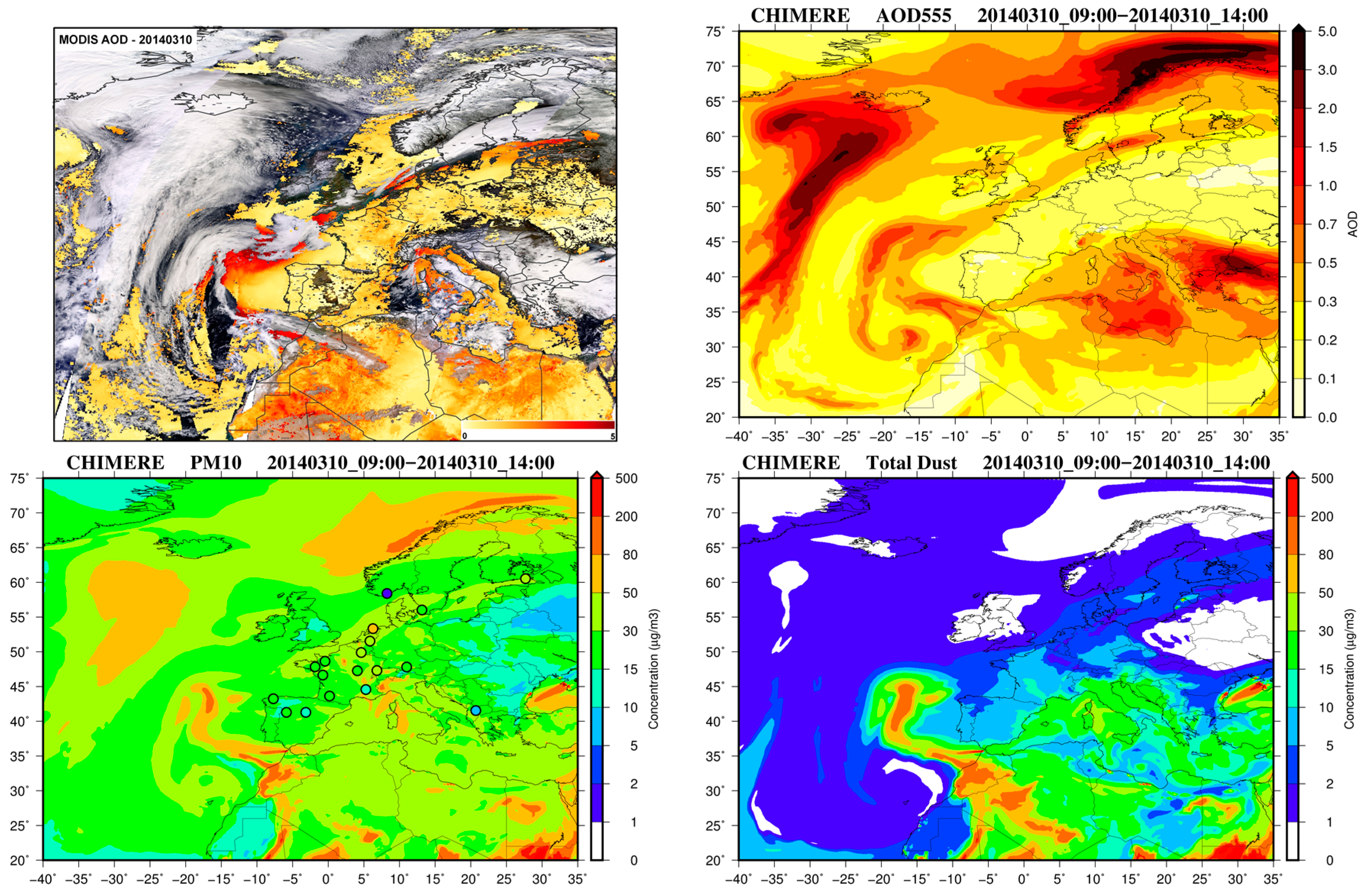
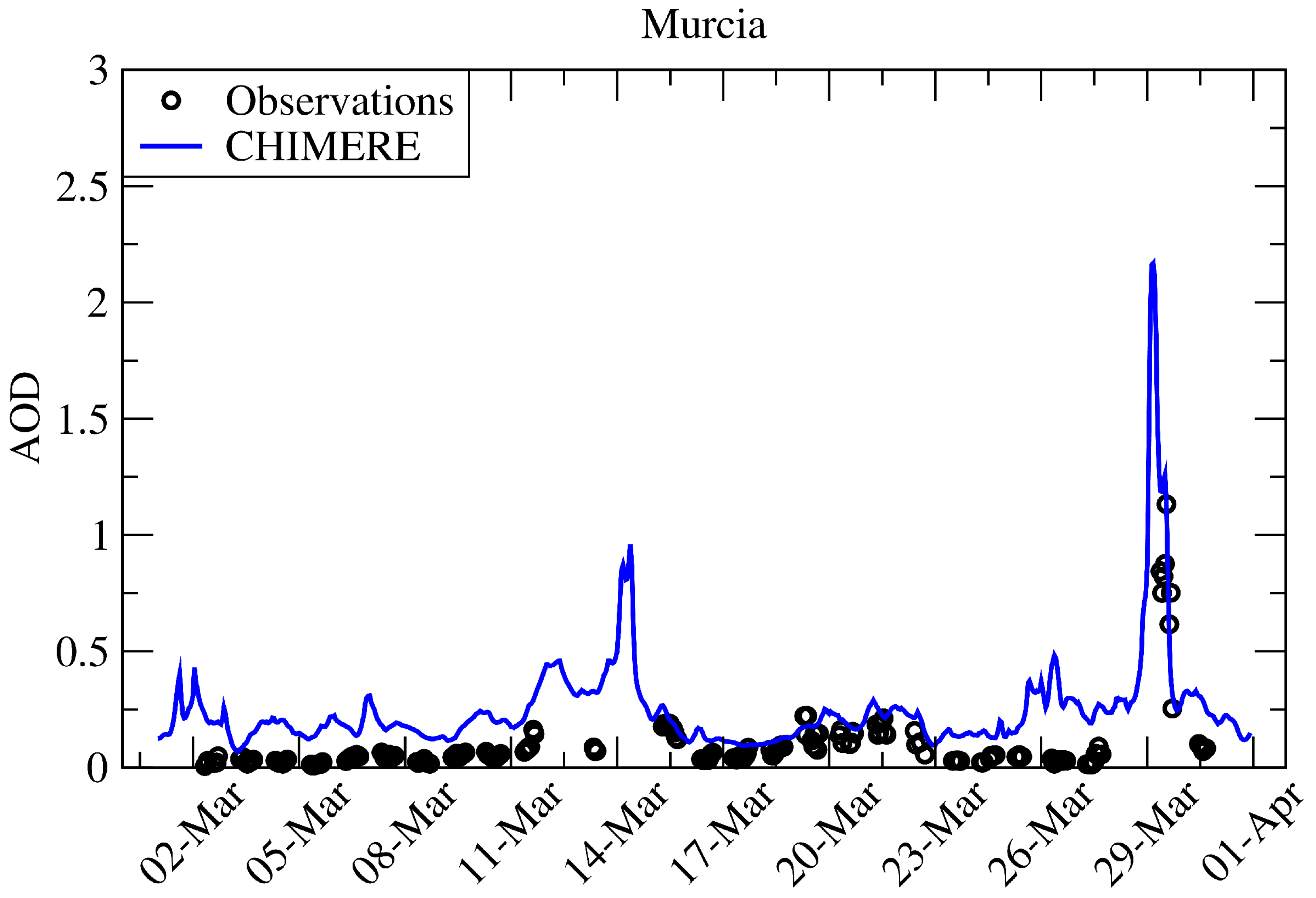
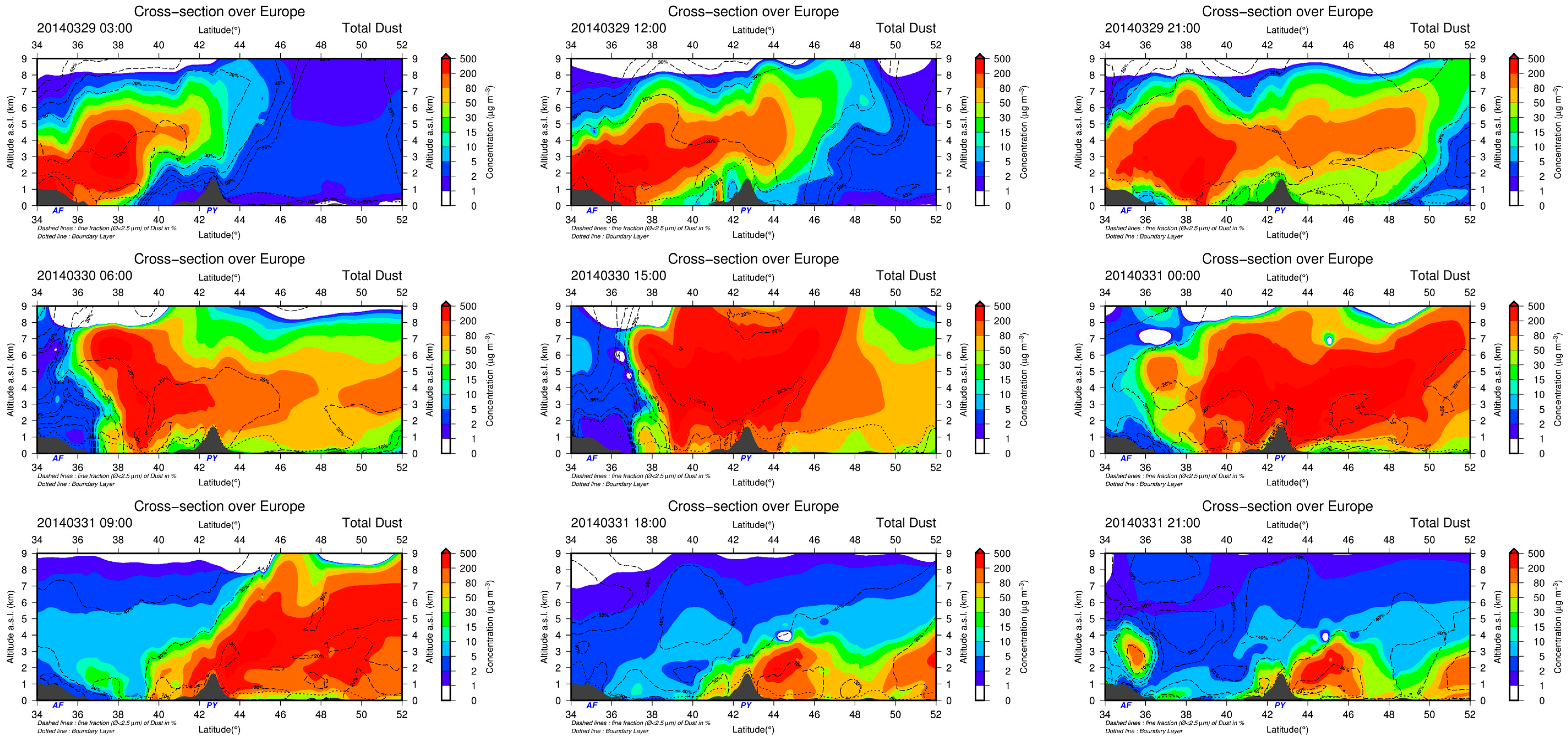
4.2. Dust Outbreaks in Europe

As mentioned in the Introduction, Europe is commonly influenced by Saharan dust outbreaks, particularly over the Mediterranean basin. France, Belgium, Netherland and Germany were affected mid-March 2014 by an important anthropogenic pollution episode due to a combination of favorable meteorological conditions and emissions from residential heating, industry, road traffic and particularly agricultural ammonia during this intensive spreading period [114]. At the end of March and beginning of April, a second episode was recorded [87]. In the early part of the episode, Saharan dust remained aloft above the UK; the presence of dust at surface level was only simulated during the second part of the episode and over a small geographic area in southern UK. The analysis presented in their study [87] illustrates the capability of air quality models, corroborated with chemically-speciated measurements, to identify the underlying causes of complex PM air pollution episodes. Specifically, the analyses highlight the substantial contribution of secondary inorganic ammonium nitrate PM, with agricultural ammonia emissions in continental Europe presenting a major driver. This event, also observed by other satellites like Meteosat-10 [115], was associated with rainfalls in UK, France and Italy. For March 2014, the time correlation of dust concentrations is quite low for the stations far from the sources but for the Mediterranean station CY0002R (Figure 13 exhibits a good correlation capturing the dust outbreaks from Africa to Asia. The Armenian station AM0001R (Figure 13) is located close to Asian emission areas and is also influenced by Saharan dust outbreaks under southwesterly air masses fluxes. However, an overestimation of predicted concentrations by the model is observed at these stations, in line with the general overestimation far from emission sources.
A spectacular dust outbreak over the Atlantic Ocean on 10 March was recorded by MODIS data as shown in Figure 14 and well captured by the model. The dust plume emitted over the Sahara was quickly ventilated in the free troposphere and blocked by high pressure systems developing over the European continental areas which led to the development of the anthropogenic pollution mid-March over the western Europe. On 10 March was the very beginning of this anthropogenic pollution event but this dust outbreak remained over the ocean in the free troposphere and partly in marine boundary layer; as shown in Figure S2 (EUR1 and EUR2 trajectories), the model captured well this event and its vertical extent up to 9 km in altitude.
The main dust outbreak, which concerns the ground level in Europe, started on 29 March with dust emitted over the Sahara. Calcium measurements (transposed in “dust” measurements by multiplying by a factor 8 [84]) confirm that the dust event was mainly confined in the free troposphere as shown by the CALIPSO data displayed in Figure S2 in Supplementary Materials. The comparison with CHIMERE (Figure 13) shows the model tends to transport a fraction of the plume within the boundary layer in several parts of Europe as supported by modeling results presented in Figure S2 in Supplementary Materials. This is confirmed at the Spanish station ES0014R close to Barcelona in the lands where dust concentrations tend to increase (Figure 13). The Murcia AERONET station (38° N–1.17° W, south of Spain) detects the dust event, the model is rather well in agreement with the observations at this station with a recorded AOD exceeding 1 and a low angstrom coefficient (close to 0) observed on 29 March confirming the coarse nature of particles (Figure 15). The time correlation between observed and modeled values is 0.85 on average for March 2014 on an hourly basis in Murcia. A pattern of high dust concentrations simulated by CHIMERE in the southwest of France and in the center of Spain can be observed in the top panel of Figure 8. Dust concentrations are generally higher in the mountainous regions certainly due to a deceleration of the dust-carrying flow [116] as it approaches the mountains with specific orographic effects around the Pyrenees leading to local peaks within the boundary layer observed in the southwest of France. Southerly air mass fluxes are associated to foehn effects over the Pyrenees, this orographic effect has been observed in China [117] leading to very stable boundary layers in the up valleys enhancing the rise of air pollutant concentrations. However, north of the Pyrenees at about 100 km, this synoptic southerly flux usually generates a southeast wind (“Autan” wind) which lowers the concentrations and explains the high boundary layer height even at night. Wind gusts up to 70 km h−1 were recorded on 29 March in Auch, a small town 100 km north of the Pyrenees (43.65° N–0.58° E), while the meteorological conditions very close to the mountains were calm with a low boundary layer height. At the EMEP background station Peyrusse Vieille about 100 km north of the Pyrenees (43.62° N–0.18° E), an increase of the coarse fraction to 35% of PM10 on 31 March compared to the days before is observed where usually the coarse fraction is in the range 20–25%. The same phenomenon is observed in Toulouse also close to the Pyrenees with a coarse fraction exceeding 50% for urban background sites on 31 March associated to an increase of PM concentrations (data are freely accessible through the French national forecasting system PREV’AIR, www.prevair.org). These potential orographic effects are captured at this resolution, with a dust plume coming from Sahara and blocked behind the Pyrenees mountain range (Figure 16).
Table 2 reports the measurements and models results at the closest station (Billere 43.31° N–0.39° E in the suburb of Pau) in the up valley of the Pyrenees and confirms an increase of concentrations with a decrease of the PM2.5/PM10 ratio confirming the presence of mineral dust in this area, although the concentrations are overestimated by the model.
Figure 17 shows the end of March 2014 evolution of hourly PM10 concentrations and mass distributions (expressed in dM/dlogDp) at the Pic du Midi station (elevation: 2876 m) located in the Pyrenees mountain range. The observed mass distribution was derived from the number distribution from 0.3 to 10 µm) using a density of 2.6 g cm−3 typical for dust [118]. The observations clearly show the sudden increase of coarse concentrations confirming the assumption of a desert dust outbreak. CHIMERE overestimates the background concentrations (before the dust event) but the timing of the dust event incidence is again rather well captured with an increase of concentrations of particles with diameter above 2.5 µm.
Far away in the north of Europe, at the Danish station DK0012R, a small signal can be detected (Figure 13), a slight increase of calcium measurements is observed and captured by the model. According to model results the dust plume extension (Figure S10 in Supplementary Materials) is simulated up to the Arctic regions on 30–31 March, unfortunately fully trustable satellite data are difficult to use to confirm this feature. Looking at AERONET version 1.5 data (cloud screened data) which were carefully used in recent works [119] compared to version 2 data (cloud screened and quality-assured data) in Figure S13 in Supplementary Materials shows a sharp increase of the AOD on 30 March which could indicate the arrival of this dust plumes at Ittoqqortoormiit station (70.48° N–21.95° E, Greenland).

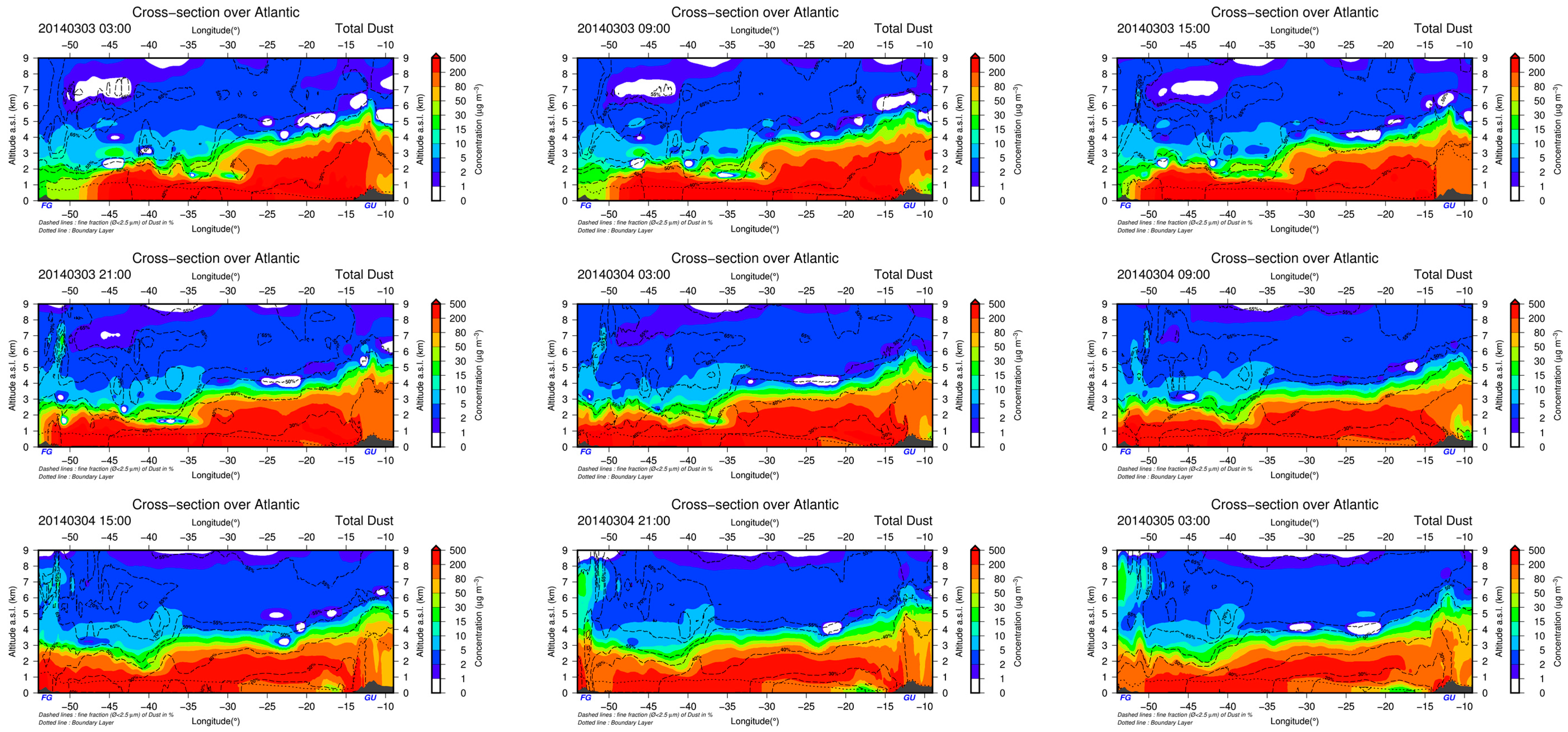
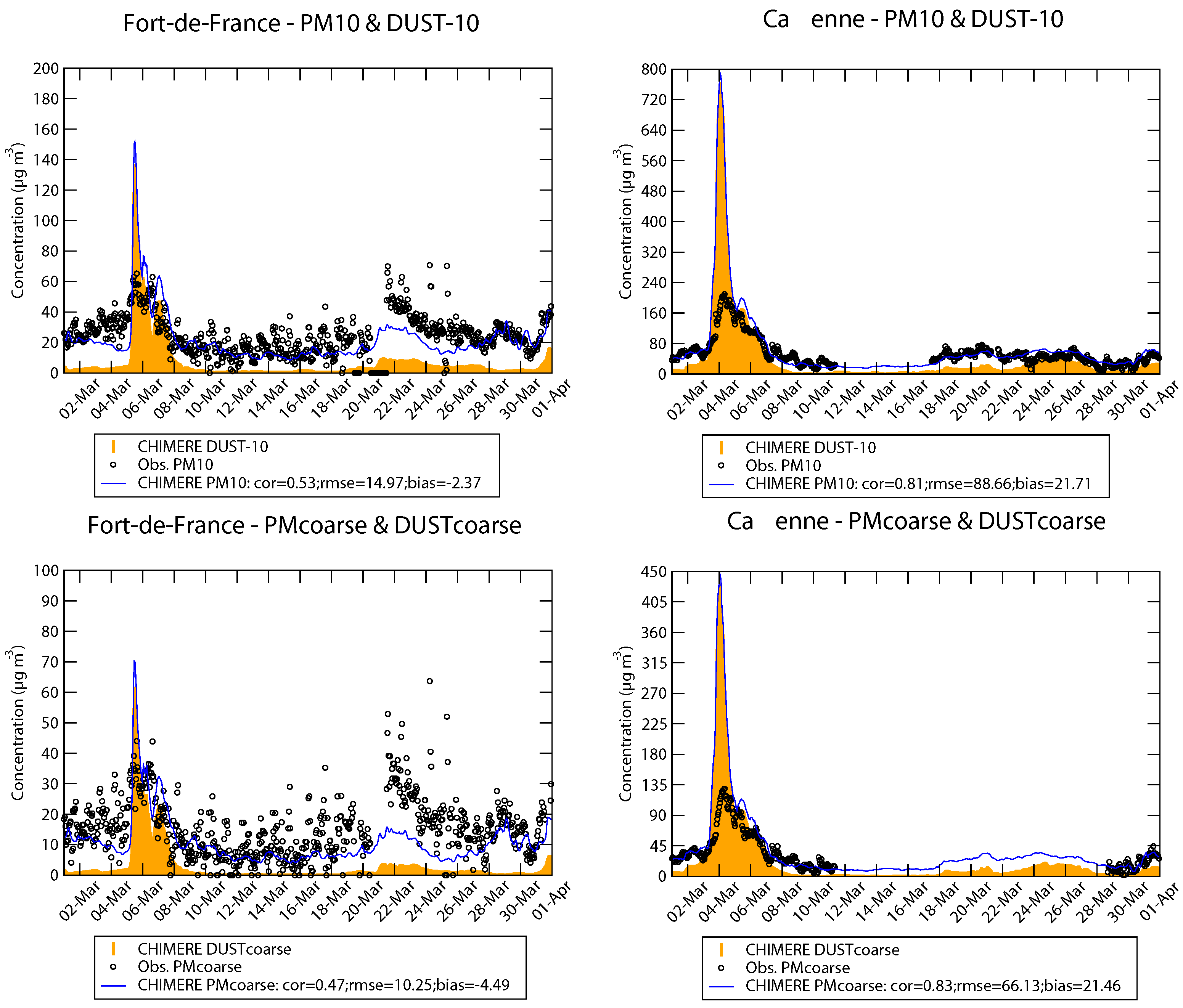
4.3. Dust Outbreaks over the Caribbean Areas

The trans-Atlantic transport of dust from Africa to the Caribbean area has been extensively reported in the literature [4,120]. Dust predictions are generally of acceptable quality for the first several days after dust emission up to 2000 km west of the African continent [121], the removal of dust from the atmosphere is too strong for large transport paths in the global models, and the simulated fine-to-coarse dust ratio (in terms of mass concentration and light extinction) is too high in the models compared to observations. This deviation is already given close to the dust sources and then increases with distance from Africa. No specific scientific publication was published so far on the recorded episodes in March 2014 over the Caribbean area.
Figure 18 shows the evolution of dust concentrations along a cross section from Guinea to the French Guiana. This transport occurs in the low troposphere and is confirmed by the latitudinal cross section issued from CALIPSO (Figure 19) and very well reproduced by the model. The increase of the boundary layer height from the African shores toward South America is related to the rise of sea surface temperature along the path (cf. global sea temperature in March 2014 reported Figure S14 in Supplementary Materials accessible at the internet NASA resource: https://neo.sci.gsfc.nasa.gov). The high boundary layer height over Africa mixes the dust within the boundary layer with a ventilation up to the free troposphere at about 5 km in altitude in this region. The fine fraction of dust increases from Africa to South America mainly due to sedimentation effects of the coarse particles but the total dust concentrations remain rather high along the pathway. The timing of the arrival on 5 and 6 March over the Caribbean is rather well captured by CHIMERE (Figure 20), however the concentration peak is overestimated. This good behavior of the model is partly due to the ability of the model to simulate the dust emission fluxes over the Sahara, the station in Cinzana close to emission sources exhibits a very good agreement between the model and observational data. The AOD simulated by CHIMERE at Dakar, Cinzana and Capo Verde stations (Figure 21) in March 2014 is very well reproduced compared to the AERONET retrievals with time correlations of 0.76, 0.70 and 0.79 respectively. A second phase of trans-Atlantic transport is observed end of March thanks to the CALIPSO data showing “dusty marine” and “dust” types of aerosols in the low troposphere also well reproduced by the model (Figure S3 in Supplementary Materials). However, the contribution attributed is low but a clear correlation can be observed between the dust load in CHIMERE and the PMcoarse measurements (Figure 20).

4.4. Dust Outbreaks in Central Asia

Dust storms are the main cause of air pollution in Central Asia, including Kazakhstan, affecting the ecology as a whole, and the health and living conditions at local levels. Dust, sand and salt storms occurring in Central Asian, Kazakhstan natural and anthropogenic deserts transport large amounts of deflated material over long distances, significantly affecting agricultural areas [122]. The drastic desiccation of the Aral Sea led to the intensive development of desertification processes in the region and the formation of a new desert, the Aralkum. In the last few decades, the Aralkum has become the new “hot spot” of dust and salt storms in the region. Dust storms and their source areas have been determined and analyzed by satellite data. An analysis of the land-cover changes in the dried bottom of the Aral Sea revealed that the northeastern part of the Aralkum Desert is one of the most active dust sources in the region, responsible for high aerosol concentrations in the atmosphere particularly in spring [123,124]. The dust source areas are identified as the Iraq–Saudi Arabia boundary region and (recently) the northwest of Iraq, using MODIS deep blue aerosol optical depth data. Subsequently, a lagged correlation was implemented between identified dust sources and whole West Asia to determine the main paths and receptors of intense dust storms. Accordingly, southwest of Iran and Persian Gulf countries were determined as main receptors of summertime dust storms in West Asia. During spring, dust storms mostly hit the northern half of the region and reach to the Caspian Sea. Analyzing atmospheric patterns, Shamal (northwesterly wind over the Middle East area) and Frontal patterns were found as dominant atmospheric circulations simultaneous with summertime and springtime dust storms, respectively [125]. In this region, a specific work described in a recent study [126] analyzed the impact of a change in horizontal distribution of emissions that lead to better simulations of dust storms with the WRF-chem model. Several studies focusing over India and Nepal agree to show the significant influence of long-range transport of dust from western desert regions, such as North Africa and the Arabic Peninsula in February–March due to changes in meteorological condition related to the starting of the Monsoon Season [127,128,129].
To our knowledge, the March 2014 dust episodes identified in our study were not reported in the scientific literature. Figure 22 shows a qualitative comparison between CALIOP-CALIPSO data and CHIMERE along the satellite passes. On 16 March, the pattern over the Arabian Peninsula is rather well reproduced by CHIMERE, the observed “dust marine” concentrations above the marine boundary layer is reproduced by the model between 10° N and 15° N in latitude. On 18 March, the satellite flies over the same regions but slightly more on the east. The two main hot spots over the Arabian Peninsula and Iran are again very well reproduced by CHIMERE, above 45° N the presence of clouds makes difficult the comparisons. On 18 March, the satellite passes west of Tehran (about 35° N) where high dust concentrations are modeled by CHIMERE, and over the west coast of the Caspian Sea with concentration peaks located above the boundary layer. The pattern simulated around 45° N located in the northwest of the Caspian Sea cannot be evaluated by CALIOP data due to the presence of clouds, it corresponds to a very emissive zone over the Volga delta, a large agricultural area (see Figure 3) where wind gusts exceeding 70 km h−1 have been recorded. On 19 and 20 March, the satellite flies over the Himalayan ranges and the comparison shows a quite good agreement between the model and observational data, the model succeeds in simulating the main patterns with high concentrations in the free troposphere up to 8000 m. Even the small structure observed by CALIOP very far from emission source areas at 77° N on 19 March is captured by the model. For the last pass (CAS6) on 30 March, the satellite flies over Iran, the dust concentration structure is again very well reproduced by the model with high concentrations captured by the model between 27° N and 55° N.
As shown in Figure 23, several meteorological SYNOP stations in central Asia recorded the presence of dust based on manned observations in the north of the Caspian Sea confirming the pattern predicted by the model in this region, unfortunately the extension of the plume toward the northeast to central and east Siberia cannot be evaluated by any measurements However, Figure 23 shows a good agreement of the manned observations with surface dust concentrations where available. The pattern in China and Mongolia over the Gobi Desert on 16 March is particularly well captured; this dust outbreak is discussed in the next section of the paper.

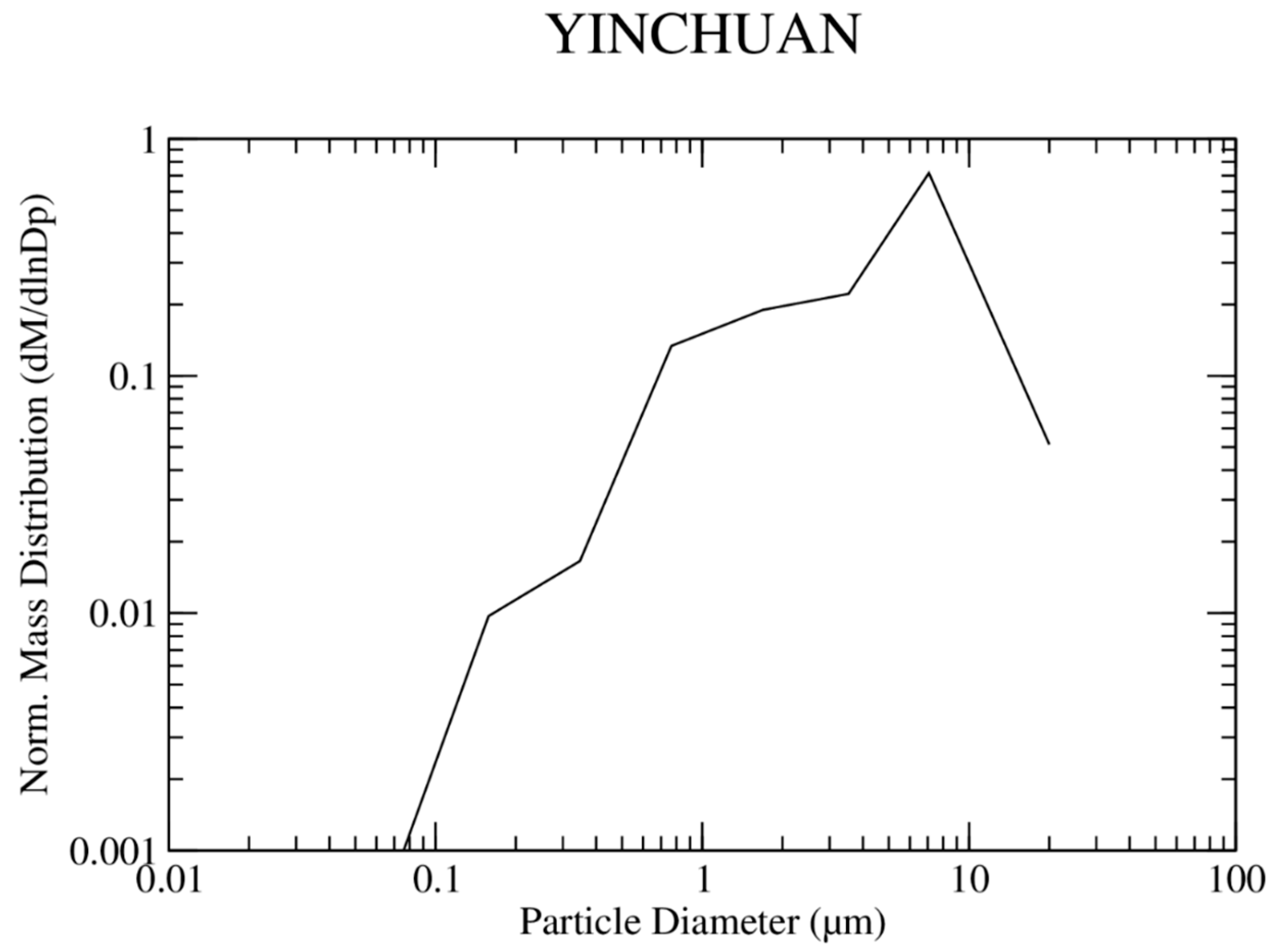
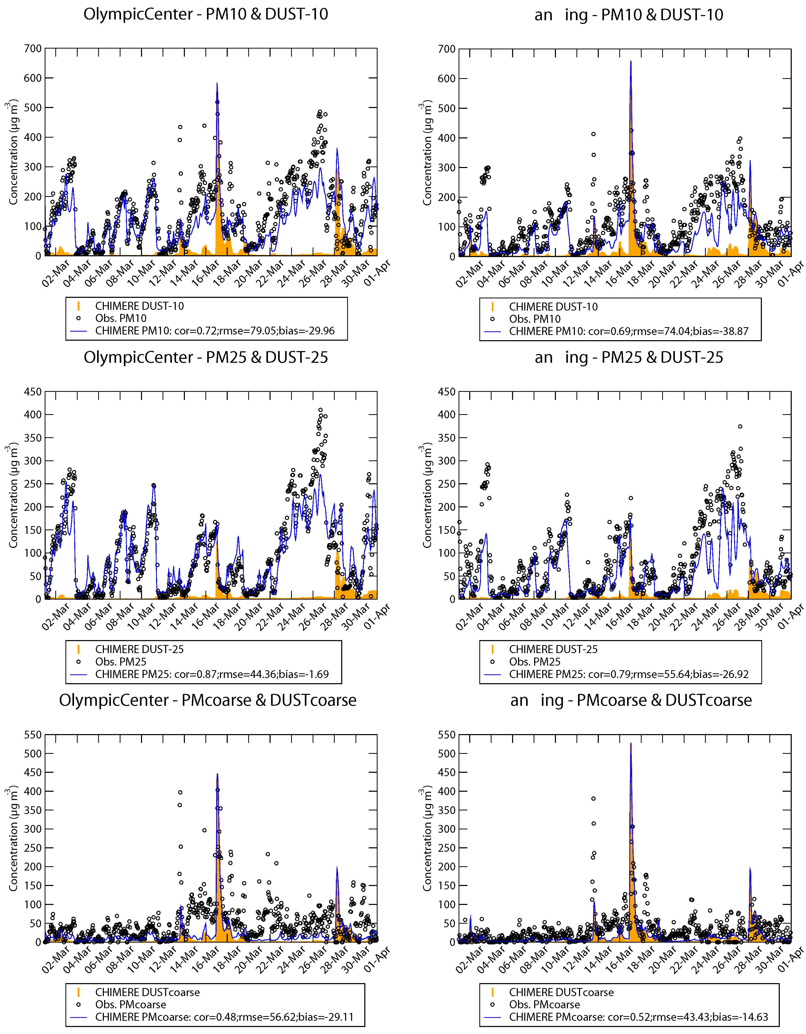
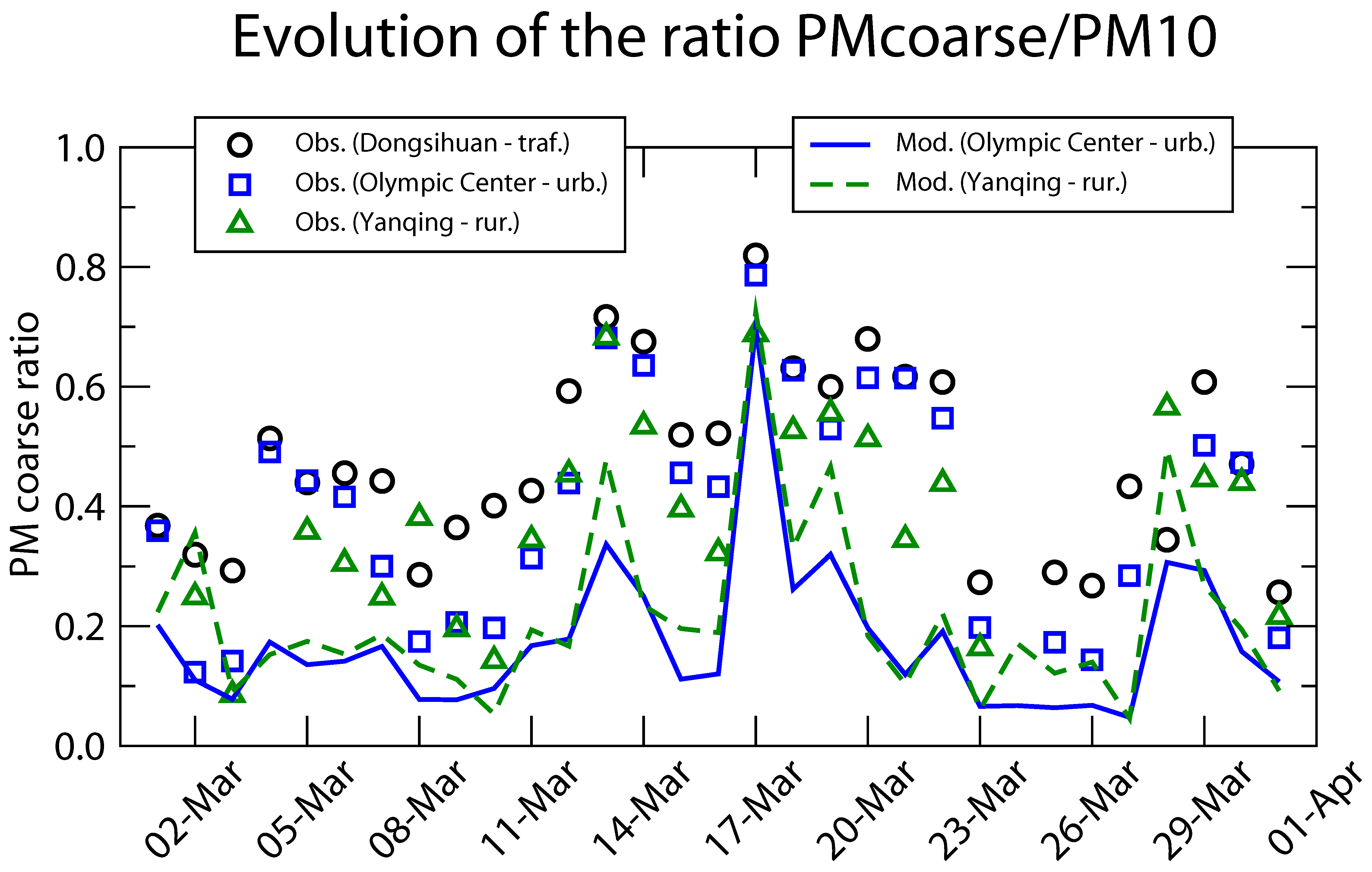
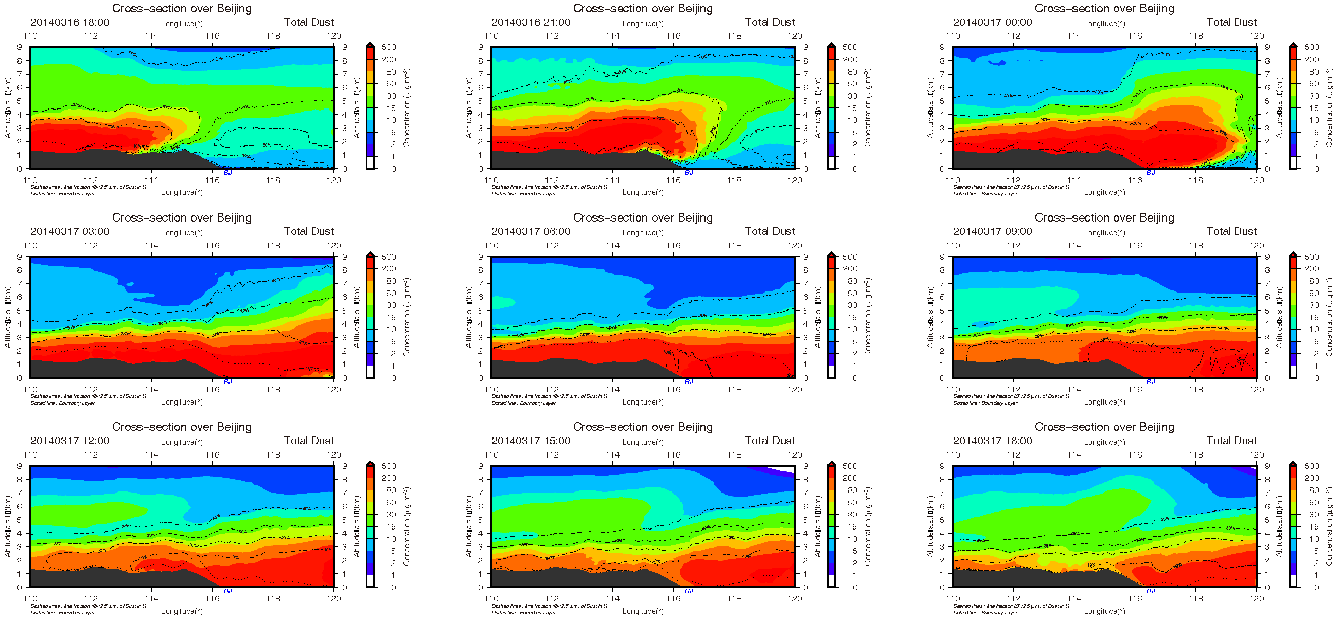
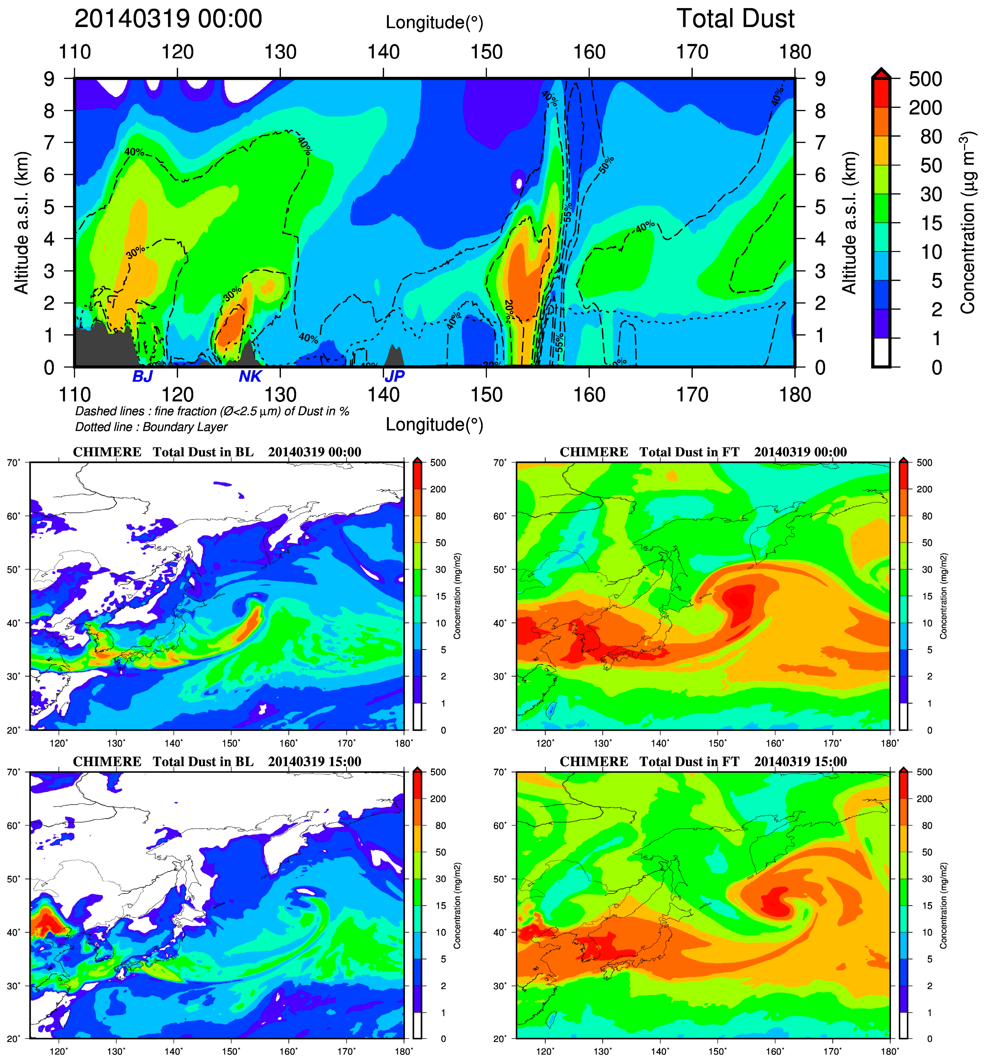
4.5. Dust Outbreaks over China

The major source areas of the Asian dust events affecting China are Gobi Desert, Taklimakan desert, and Loess Plateau [130,131,132]. Two major dust outbreaks affecting the region of Beijing are identified in 12–13 and 16–18 March 2014, another episode also identified end of March. Figure 24 shows a comparison between CHIMERE concentrations and CALIPSO qualitative data passing over the east part of China. The shape of dust concentrations is very well reproduced by CHIMERE and extends up to 5 and 6 km in altitude then largely ventilated into the free troposphere.
The March 2014 episodes were discussed in previous studies [133,134], to understand the long-range transport processes of bioaerosols over the Asian-dust source regions. The mid-March episode was also studied with satellites data issued from CALIPSO to track the trans-Pacific transport of dust from Asia to North America [135]. These episodes were also studied by using a global model [136]; they confirmed the importance of coarse-mode dust-nitrate as evidence of “polluted dust” event. The model analysis showed that the formation of dust-nitrate occurred over the Yellow Sea and East China Sea before arriving in Japan. The mid-March episode was studied with the on-line coupled Weather Research and Forecasting-Chemistry (WRF-Chem) model over the Nanjing area focusing on the interactions between the dust load with the photochemistry [137]. Combined with observational data, the WRF-chem model has been recently used in a recent study [138] at 1° × 1° to analyze the transport of a dust plume from Asia to North America for an episode in March 2015. They show the dust plume located in the altitudes ranging from 1 km to 7 km over the source region, then ascended to 2–9 km over the Pacific Ocean. High wind speed enhancing the height of planetary boundary layer (PBL) tend to occur in spring over northern China [139], which are favorable for the dust particles to be lofted into the free troposphere. These events were also analyzed in terms of emissions size distributions in Yinchuan, China close to Inner Mongolia [140], showing a bi-modal emission shape of the mass particle size distributions (PSD), but very different according their emission conditions (background, floating dust, blowing dust, and dust storm), these two modes are located at 3–4 µm and around 10 µm in diameter. However, from in situ measurements compiled close to North African source regions [141], an emission mode is usually observed around 10 µm. From campaign to campaign the PSD are very different [142] since they depend on the location of measurements and meteorological conditions. Other studies report particle size distribution curves of Asian dust often extending over 10 μm. In a previous study [143], a mean diameter of about 9 μm by using a cascade impactor in Seoul was reported. CHIMERE (Figure 25) displays only one mode around 10 µm in Yinchuan, the missing first peak could be explained by an underestimation of the anthropogenic fraction of PM2.5 in the model due to a lack of emissions in the model for this city.
As shown in Figure 26, the ratio PMcoarse/PM10 exceeds 50–60% during the previous identified episode; this threshold is usually mentioned to identify a mineral dust outbreak [16]. On average, the model captures quite well the evolution of PM concentrations over the Beijing area in March 2014 (Figure 27), the correlation is close to 0.8 for most of stations either for PM2.5 and PM10 concentrations with a very low bias. However, the coarse fraction seems underestimated by the model (Figure 26). The dust outbreaks impacting Beijing can be identified by the predicted dust concentrations with a sudden rise of PM concentrations particularly the PMcoarse fraction on 17 March peaking at 400 µg m−3 on an hourly basis over Beijing. Under less “dusty” conditions at the beginning of March, this coarse fraction is largely below 50 µg m−3. During the 17 March episode, the coarse fraction in the observations reaches 70% of PM10 daily compared to a model value of 72% in Yanqing near Beijing. A last dust episode at the end of March occurs in the simulation outputs starting at the end of an anthropogenic episode which took place between 22 and 27 March over Beijing. On 28 March, the CALIPSO data reveals the starting point of this dust episode over the Gobi Desert (Figure S5 in Supplementary Material, CNA5 trajectory) and a slight increase of coarse PM concentrations are observed at the rural station Yanqing. At this station, the coarse fraction reaches 50% on 28 March in the model compared to less than 20% the days before during the anthropogenic pollution episode, this fraction is even larger in the observations reaching 60%. A closer look at the observations in Figure 26 shows that CHIMERE simulates higher coarse fraction ratio for rural stations compared to the urban station while the observations show the opposite with the highest values at the traffic station. This reveals the importance of dust resuspension over the cities. Particles emitted from anthropogenic (road traffic, urban works, other human activities, etc.) or natural processes (windy conditions on flat surfaces) can lead to more dust in urban areas compared to nearby rural zones. These latter processes are not included or activated in CHIMERE for this study.
The evolution of the dust plumes over Beijing is displayed in Figure 28 which shows the evolution of concentrations along a longitudinal cross section passing over the capital of China. The dust comes from the Mongolian Plateau (1000–1500 m a.s.l.), the Gobi Desert being the main source of this episode. The model simulates concentrations largely above 500 µg m−3 inside the plume that is located mainly within the boundary layer when hitting Beijing on 17 March. The dust plumes are advected up to the Pacific Ocean; their transport occurs mainly in the free troposphere as shown in Figure 29. The role of the topography (Japan and North Korean mountain ranges) is certainly of major importance to lift the dust up to the top of the boundary layer and drive their injection within the free troposphere. The contribution of the topography on air pollutant dispersion in this region has already been identified in previous studies [144]. Other processes are dominant in the vertical redistribution of pollution in the mid latitudes: frontal activity and deep convection are usually identified, for instance the frontal systems, especially the so-called warm conveyor belts (WCBs) associated with extratropical cyclones. The role of the WCB is considered as the dominant advective transport mechanism for boundary-layer ventilation and transport of air pollutants into the free troposphere [139,145] and confirmed in a study in Asia for a specific dust event [146]. Our simulation reveals very fine structures of the desert dust conveyed by the WCB even if these processes are large-scale events (Figure 29). In the AeroCom Project [104], simulations with global models run at coarse resolutions show how the boundary-layer mixing plays a dominant role for sea salt and mineral dust, which are emitted only from the surface, dry deposition and below-cloud scavenging were identified as important processes for the vertical distribution of mineral dust. On 19 March 15:00 UTC, low dust concentrations integrated over the boundary layer can be observed in the center of the cyclonic structure in relation with the sharp decrease of the marine boundary layer. During the studied period, a series of low-pressure systems over the Pacific lifts the dust plumes up to the free troposphere. This transport of dust in the free troposphere far away over the Pacific Ocean is confirmed by the CALIPSO data shown in Figure S15 in Supplementary Materials with a dust plume located between 4 and 6 km in altitude very well reproduced by CHIMERE.

5. Conclusions

A wide variety of observational data (satellite and ground based measurements) has been used to evaluate the ability of the chemistry transport model CHIMERE to simulate dust outbreaks through the Northern Hemisphere in March 2014. The novelty of this work is to use a regional chemistry transport model (CHIMERE) at such a large scale with a high resolution (about 10 km), focusing on several places in the world for the same short period, and evaluating simultaneously the ability of the model to simulate these episodes.
The CHIMERE model can simulate the main patterns of the dust concentrations compared to previous modeling studies and produces much more detailed structures due to the very fine horizontal resolution. Over mid latitudes, the transport of dust in low free troposphere is confirmed particularly over the Pacific Ocean while the transatlantic transport of dust from Sahara to the Caribbean area mainly occurs within the boundary layer. Close to the equatorial Pacific and Atlantic Oceans the fine fraction of dust concentration is dominating due to heavy precipitations which efficiently remove the biggest particles by sub-cloud scavenging. The background dust concentrations seem overestimated by the model when comparing the data at high latitude sites. A specific pattern is simulated with high dust concentrations over the pole at about 2–3 km in altitude, which is certainly the result of dust accumulation issued from long-range transport. In the model, the effect of sedimentation for the biggest particles and the condensation and coagulation of the smallest aerosols shows a narrowing of the size aerosol distributions toward the upper levels of the atmosphere.
Several dust outbreaks have been identified in March 2014; some of them, already studied in previous works, are very well captured by the model with a good timing. In China, the three main events are very well simulated, the model outputs showing a sharp increase of PM concentrations over the Beijing area due to dust issued from the Gobi Desert. Over the USA, three dust storms have been identified and analyzed with several observational datasets and CHIMERE is able to simulate these events with a rather good timing. The evolution of the plumes toward Mexico and particularly Baja California is confirmed by available observations. Europe is mainly affected during end of March with a dust plume that is mainly located in the free troposphere at the beginning with some intrusions within the boundary layer; this episode affects later in April the UK [87]. The Caribbean area is affected by a long-range transport of dust from the Sahara and again the model rather well captures the arrival timing of the plume but with a clear overestimation while the concentrations and AOD are in rather good agreement on African stations. The transport of dust in the low troposphere is confirmed by CALIPSO retrievals. Over Asia, several dust episodes are also identified and rather well captured by the model. Unfortunately, the difficulty to obtain PM measurements in Siberia and the impossibility to use satellite data due to the presence of clouds makes difficult the evaluation of the model, however the SYNOP manned measurements confirmed the evolution of the dust plumes in Central Asia.
While the timing of dust outbreaks is rather well simulated, one identified shortcoming of CHIMERE is the difficulty to simulate the background concentrations and the magnitude of dust concentrations far from emission source areas. Additional improvements must be performed to better simulate the lowest concentration values far from emission areas which seems overestimated. Processes such as wet deposition will be revised in the next version of CHIMERE to improve the model results. The implementation of a more complete aqueous chemistry module is also one of the next challenges of the developments for the CHIMERE community [147]. The evolution of the size distribution has to be better analyzed in the next studies. The nitrate coating of coarse mineral particles could also influence their removal [148,149]; this process must be implemented in the next version of the model. In addition, the capacity of the model to transport thin dust layers has to be improved, indeed the chemistry transport models tend to vertically diffuse the dust within the boundary layer and the free troposphere, more layers has to be implemented in CHIMERE in accordance with the available layers in the meteorological model driver. This issue has been recently studied [150], the long-range transport of pollutants is improved by an increase of vertical resolution; 100 m layers in the free troposphere is expect to favor a more realistic transport of thin dust layers, even if CHIMERE displayed a rather good ability to simulate the vertical profile of dust concentrations [151]. An improvement of the vertical resolution within the boundary layer seems less important [152], except close to the ground where the roughness plays an important role on the local dispersion of emitted pollutants. As identified in recent studies [153], the interactions of dust with meteorology through the radiative budget have also a strong influence on the emissions and diffusion within the boundary layer justifying the current work on a full-coupled version of CHIMERE with a mesoscale meteorological model [3]. These interactions must be considered between dust, clouds and chemical processes, which could influence the chemical regimes of trace elements in cloud droplets [154]. At the urban scale, the resuspension processes of natural dust or issued from anthropogenic activities (industries, constructions, road traffic, etc.) must be revisited in CHIMERE, particularly to better simulate the PM10 concentrations in urban areas influenced by dry climatic conditions such as Beijing in early spring before the rainy season.

Supplementary Materials

The following Supplementary Materials are available online at www.mdpi.com/2073-4433/8/12/251/s1, Table S1. Error statistics (Correlation, Root Mean Square Error-RMSE, Bias) for CHIMERE at several AERONET stations over the Northern Hemisphere for March 2014; Table S2. Characteristics, locations of EBAS-EMEP sites used in this study; Figure S1. Cross sections of CHIMERE dust concentrations (right) for several orbits zoomed over the highest values area versus the corresponding CALIPSO qualitative data (left) showing in yellow the dust load and in orange the polluted dust, for the CALIPSO trajectories NAM1-6 as reported in Figure 2 in the publication. The dotted line represents the height of the boundary layer, the dashed lines represent the fraction of fine dust in percent; Figure S2. Cross sections of CHIMERE dust concentrations (right) for several orbits zoomed over the highest values area versus the corresponding CALIPSO qualitative data (left) showing in yellow the dust load and in orange the polluted dust, for the CALIPSO trajectories EUR1-5 as reported in Figure 2 in the publication. The dotted line represents the height of the boundary layer, the dashed lines represent the fraction of fine dust in percent; Figure S3. Cross sections of CHIMERE dust concentrations (right) for several orbits zoomed over the highest values area versus the corresponding CALIPSO qualitative data (left) showing in yellow the dust load and in orange the polluted dust, for the CALIPSO trajectories CAR1-6 as reported in Figure 2 in the publication. The dotted line represents the height of the boundary layer, the dashed lines represent the fraction of fine dust in percent; Figure S4. Cross sections of CHIMERE dust concentrations (right) for several orbits zoomed over the highest values area versus the corresponding CALIPSO qualitative data (left) showing in yellow the dust load and in orange the polluted dust, for the CALIPSO trajectories CAS1-6 as reported in Figure 2 in the publication. The dotted line represents the height of the boundary layer, the dashed lines represent the fraction of fine dust in percent. Figure S5. Cross sections of CHIMERE dust concentrations (right) for several orbits zoomed over the highest values area versus the corresponding CALIPSO qualitative data (left) showing in yellow the dust load and in orange the polluted dust, for the CALIPSO trajectories CNA1-6 as reported in Figure 2 in the publication. The dotted line represents the height of the boundary layer, the dashed lines represent the fraction of fine dust in percent; Figure S6. Map of site locations presented in the publication for: AERONET stations (a); IMPROVE stations (b); US EPA networks for PM2.5 data (c); EBAS-EMEP stations (d) (see Table S2 for the names of EMEP stations); French stations close to the Pyrenees area (e); Chinese stations (f); and the two stations in the Caribbean area (g); Figure S7. Evolution of mean daily concentrations integrated over the column (in g m−2) of total dust from 1 to 8 March 2014 in the free troposphere (FT) and the boundary layer (BL); Figure S8. Evolution of mean daily concentrations integrated over the column (in g m−2) of total dust from 9 to 16 March 2014 in the free troposphere (FT) and the boundary layer (BL); Figure S9. Evolution of mean daily concentrations integrated over the column (in g m−2) of total dust from 17 to 24 March 2014 in the free troposphere (FT) and the boundary layer (BL); Figure S10. Evolution of mean daily concentrations integrated over the column (in g m−2) of total dust from 25 to 31 March 2014 in the free troposphere (FT) and the boundary layer (BL); Figure S11. Monthly mean latitudinal cross sections (Altitude a.g.l. versus Latitude °N) for several variables in March 2014 simulated by CHIMERE over the Northern Hemisphere. Top panels represent the mean dust concentrations with bold dashed lines representing the fine fraction of total dust (%), the grey dotted lines are the average zonal winds (conventionally, westerly wind are positive). Bottom charts represent the evolution of various parameters along the corresponding cross sections and spatially averaged over the longitude: the boundary layer (BL) height in km, the total precipitation (convective and large scale) in cm month−1, the deep convection updraft flux summed over the column in gair m−2 s−1, the mean cloud water content averaged over the first 10 model layers (approximatively 2500 m), the wet and dry deposition fluxes of dust sum over time (monthly) in mgdust m−2 month−1 and the ratio Ω (unit less) of dry (d) and wet (w) scavenging coefficients coarse versus fine particles as defined in Equation (2) in the publication) ; Figure S12. PM2.5 time series at Chihuahua station (Mexico) for CHIMERE and the corresponding observations. The orange shade area represents the dust in the PM2.5 matrix simulated by CHIMERE; Figure S13. AOD from AERONET network at Ittoqqortoomitt in March 2014, level 1.5 (left) and level 2 (right) (source: NASA, https://aeronet.gsfc.nasa.gov/); Figure S14. Mean sea surface temperature in March 2014 (source: NASA https://worldview.earthdata.nasa.gov); Figure S15. Cross sections of CHIMERE dust concentrations (right) for several orbits zoomed over the highest values area versus the corresponding CALIPSO qualitative data (left) showing in yellow the dust load and in orange the polluted dust, for the CALIPSO trajectories PAC-1-2 as reported in Figure 2 in the publication. The dotted line represents the height of the boundary layer, the dashed lines represent the fraction of fine dust in percent; Figure S16. Longitudinal cross section of total dust concentrations fields (Altitude versus longitude) at 39.9° N latitude from 110° E to 120° E passing over Beijing (BJ in blue letters) from 12 March 00:00 UTC to 15 March 21:00 UTC. The dotted line represents the height of the boundary layer, the dashed lines represent the fraction of fine dust in percent; Figure S17. Longitudinal cross section of total dust concentrations fields (Altitude versus longitude) at 39.9° N latitude from 110° E to 120° E passing over Beijing (BJ in blue letters) from 16 March 00:00 UTC to 19 March 21:00 UTC. The dotted line represents the height of the boundary layer, the dashed lines represent the fraction of fine dust in percent.

Acknowledgments

This work is partly funded by the French Ministry in charge of Ecology (MTES). IMPROVE is a collaborative association of state, tribal, and federal agencies, and international partners. US Environmental Protection Agency is the primary funding source, with contracting and research support from the National Park Service. The Air Quality Group at the University of California, Davis is the central analytical laboratory, with ion analysis provided by Research Triangle Institute, and carbon analysis provided by Desert Research Institute. The EBAS database has largely been funded by the UN-ECE CLRTAP (EMEP), AMAP and through NILU internal resources. Specific developments have been possible due to projects like EUSAAR (EU-FP5) (EBAS web interface), EBAS-Online (Norwegian Research Council INFRA) (upgrading of database platform) and HTAP (European Commission DG-ENV) (import and export routines to build a secondary repository in support of www.htap.org). Many specific projects have supported development of data and meta data reporting schemes in dialog with data providers (EU) (CREATE, ACTRIS and others). For a complete list of programmes and projects for which EBAS serves as a database, please consult the information box in the Framework filter of the web interface. These are all highly acknowledged for their support. CALIPSO data are archived and distributed by the Atmospheric Science Data Center (ASDC) at NASA Langley Research Center that is responsible for the processing, archival, and distribution of NASA Earth science data in the areas of radiation budget, clouds, aerosols, and tropospheric composition. The high-performance computing facility and staff at CCRT/CEA is gratefully acknowledged. We thank also Terry Keating for advising us on the use of US air quality data. We acknowledge the Pyrenean Platform for Observation of the Atmosphere (P2OA, http://p2oa.aero.obs-mip.fr) for the data collected at the Pic du Midi in the frame of the SNO (Service National d’ Observation) CLAP supported by the CNRS (Centre National de la Recherche Scientifique). P2OA facilities and staff are funded and supported by the Observatoire Midi-Pyrénées (University Paul Sabatier, Toulouse, France), and CNRS.

Author Contributions

Bertrand Bessagnet coordinated the study and performed most of the final simulations and wrote a large part of the paper. Laurent Menut developed post-processing tools and was in charge of the development of the dust module. He contributed to writing the paper. Augustin Colette was in charge of the model set-up, performed the preliminary simulations and coordinated the pre-project leading to this study. Florian Couvidat was in charge of the model set-up and anthropogenic emissions. Mo Dan was in charge of the analysis over Beijing and collected data in China and data processing. Sylvain Mailler was in charge of the preliminary simulations at the hemispheric scale. Laurent Létinois was in charge of data processing particularly for the satellites data. Véronique Pont worked on the data processing and analysis issued from the Pic-du-Midi observatory. Laurence Rouïl has participated to the analysis of the episodes and contributed to writing the paper.

Conflicts of Interest

The authors declare no conflict of interest.

References

  1. WHO Regional Office for Europe, OECD. Economic Cost of the Health Impact of Air Pollution in Europe: Clean Air, Health and Wealth; WHO Regional Office for Europe: Copenhagen, Denmark, 2015. [Google Scholar]
  2. Ding, L.; Zhu, D.; Peng, D.; Zhao, Y. Air pollution and asthma attacks in children: A case–crossover analysis in the city of Chongqing, China. Environ. Pollut. 2017, 220, 348–353. [Google Scholar] [CrossRef] [PubMed]
  3. Briant, R.; Tuccella, P.; Deroubaix, A.; Khvorostyanov, D.; Menut, L.; Mailler, S.; Turquety, S. Aerosol-radiation interaction modeling using online coupling between the WRF 3.7.1 meteorological model and the CHIMERE 2016 chemistry-transport model, through the OASIS3-MCT coupler. Geosci. Model Dev. 2017, 10, 927–944. [Google Scholar] [CrossRef]
  4. Weinzierl, B.; Ansmann, A.; Prospero, J.M.; Althausen, D.; Benker, N.; Chouza, F.; Dollner, M.; Farrell, D.; Fomba, W.K.; Freudenthaler, V.; et al. The Saharan Aerosol Long-range TRansport and Aerosol Cloud Interaction Experiment (SALTRACE): Overview and selected highlights. Bull. Am. Meteorol. Soc. 2017, 98, 1428–1451. [Google Scholar] [CrossRef]
  5. Fuzzi, S.; Baltensperger, U.; Carslaw, K.; Decesari, S.; Denier van der Gon, H.; Facchini, M.C.; Fowler, D.; Koren, I.; Langford, B.; Lohmann, U.; et al. Particulate matter, air quality and climate: Lessons learned and future needs. Atmos. Chem. Phys. 2015, 15, 8217–8299. [Google Scholar] [CrossRef] [Green Version]
  6. Middleton, N.J. Desert dust hazards: A global review. Aeolian Res. 2017, 24, 53–63. [Google Scholar] [CrossRef]
  7. Bessagnet, B.; Menut, L.; Aymoz, G.; Chepfer, H.; Vautard, R. Modeling dust emissions and transport within Europe: The Ukraine March 2007 event. J. Geophys. Res. 2008, 113, D15202. [Google Scholar] [CrossRef]
  8. Pérez García-Pando, C.; Stanton, M.C.; Diggle, P.J.; Trzaska, S.; Miller, R.L.; Perlwitz, J.P.; Baldasano, J.M.; Cuevas, E.; Ceccato, P.; Yaka, P.; et al. Soil dust aerosols and wind as predictors of seasonal meningitis incidence in Niger. Environ. Health Perspect. 2014, 122, 679–686. [Google Scholar] [CrossRef] [PubMed]
  9. Ghio, A.J.; Kummarapurugu, S.T.; Tong, H.; Soukup, J.M.; Dailey, L.A.; Boykin, E.; Gilmour, M.I.; Ingram, P.; Roggli, V.L.; Goldstein, H.L.; et al. Biological effects of desert dust in respiratory epithelial cells and a murine model. Inhal. Toxicol. 2014, 26, 299–309. [Google Scholar] [CrossRef] [PubMed]
  10. Jusot, J.-F.; Neill, D.R.; Waters, E.M.; Bangert, M.; Collins, M.; Bricio Moreno, L.; Lawan, K.G.; Moussa Moussa, M.; Dearing, E.; Everett, D.B.; et al. Airborne dust and high temperatures are risk factors for invasive bacterial disease. J. Allergy Clin. Immunol. 2017, 139, 977–986.e2. [Google Scholar] [CrossRef] [PubMed]
  11. Stafoggia, M.; Zauli-Sajani, S.; Pey, J.; Samoli, E.; Alessandrini, E.; Basagaña, X.; Cernigliaro, A.; Chiusolo, M.; Demaria, M.; Díaz, J.; et al. Desert dust outbreaks in Southern Europe: Contribution to daily PM10 concentrations and short-term associations with mortality and hospital admissions. Environ. Health Perspect. 2016, 124, 413–419. [Google Scholar] [CrossRef] [PubMed]
  12. Kanatani, K.T.; Ito, I.; Al-Delaimy, W.K.; Adachi, Y.; Mathews, W.C.; Ramsdell, J.W. Desert dust exposure is associated with increased risk of asthma hospitalization in children. Am. J. Respir. Crit. Care Med. 2010, 182, 1475–1481. [Google Scholar] [CrossRef] [PubMed]
  13. Yoo, Y.; Choung, J.T.; Yu, J.; Kim, D.K.; Koh, Y.Y. Acute effects of Asian dust events on respiratory symptoms and peak expiratory flow in children with mild asthma. J. Korean Med. Sci. 2008, 23, 66–71. [Google Scholar] [CrossRef] [PubMed]
  14. Thalib, L.; Al-Taiar, A. Dust storms and the risk of asthma admissions to hospitals in Kuwait. Sci. Total Environ. 2012, 433, 347–351. [Google Scholar] [CrossRef] [PubMed]
  15. Wang, C.-H.; Chen, C.-S.; Lin, C.-L. The threat of Asian dust storms on asthma patients: A population-based study in Taiwan. Glob. Public Health 2014, 9, 1040–1052. [Google Scholar] [CrossRef] [PubMed]
  16. Perez, L.; Tobias, A.; Querol, X.; Kunzli, N.; Pey, J.; Alastuey, A.; Viana, M.; Valero, N.; Gonzalez-Cabre, M.; Sunyer, J. Coarse particles from Saharan dust and daily mortality. Epidemiology 2008, 19, 800–807. [Google Scholar] [CrossRef] [PubMed]
  17. UNEP, WMO, UNCCD Global Assessment of Sand and Dust Storms. United Nations Environment Programme, Nairobi. 2016. Available online: http://www.unep.org/publications (accessed on 17 August 2017).
  18. Marinou, E.; Amiridis, V.; Binietoglou, I.; Tsikerdekis, A.; Solomos, S.; Proestakis, E.; Konsta, D.; Papagiannopoulos, N.; Tsekeri, A.; Vlastou, G.; et al. Three-dimensional evolution of Saharan dust transport towards Europe based on a 9-year EARLINET-optimized CALIPSO dataset. Atmos. Chem. Phys. 2017, 17, 5893–5919. [Google Scholar] [CrossRef]
  19. Barnaba, F.; Bolignano, A.; Di Liberto, L.; Morelli, M.; Lucarelli, F.; Nava, S.; Perrino, C.; Canepari, S.; Basart, S.; Costabile, F.; et al. Desert dust contribution to PM10 loads in Italy: Methods and recommendations addressing the relevant European Commission Guidelines in support to the Air Quality Directive 2008/50. Atmos. Environ. 2017, 161, 288–305. [Google Scholar] [CrossRef]
  20. Tong, D.Q.; Dan, M.; Wang, T.; Lee, P. Long-term dust climatology in the western United States reconstructed from routine aerosol, ground monitoring. Atmos. Chem. Phys. 2012, 12, 5189–5205. [Google Scholar] [CrossRef]
  21. Tong, D.Q.; Wang, J.X.L.; Gill, T.E.; Lei, H.; Wang, B. Intensified dust storm activity and Valley fever infection in the southwestern United States. Geophys. Res. Lett. 2017, 44, 4304–4312. [Google Scholar] [CrossRef]
  22. Tagliabue, A.; Bowie, A.R.; Boyd, P.W.; Buck, K.N.; Johnson, K.S.; Saito, M.A. The integral role of iron in ocean biogeochemistry. Nature 2017, 543, 51–59. [Google Scholar] [CrossRef] [PubMed]
  23. Herut, B.; Rahav, E.; Tsagaraki, T.M.; Giannakourou, A.; Tsiola, A.; Psarra, S.; Lagaria, A.; Papageorgiou, N.; Mihalopoulos, N.; Theodosi, C.N.; et al. The Potential Impact of Saharan Dust and Polluted Aerosols on Microbial Populations in the East Mediterranean Sea, an Overview of a Mesocosm Experimental Approach. Front. Mar. Sci. 2016, 3, 226. [Google Scholar] [CrossRef]
  24. Tozer, P.; Leys, J. Dust storms—What do they really cost? Rangel. J. 2013, 35, 131–142. [Google Scholar] [CrossRef]
  25. Huneeus, N.; Basart, S.; Fiedler, S.; Morcrette, J.-J.; Benedetti, A.; Mulcahy, J.; Terradellas, E.; Pérez García-Pando, C.; Pejanovic, G.; Nickovic, S.; et al. Forecasting the Northern African dust outbreak towards Europe in April 2011: A model intercomparison. Atmos. Chem. Phys. 2016, 16, 4967–4986. [Google Scholar] [CrossRef] [Green Version]
  26. Lu, C.-H.; da Silva, A.; Wang, J.; Moorthi, S.; Chin, M.; Colarco, P.; Tang, Y.; Bhattacharjee, P.S.; Chen, S.-P.; Chuang, H.-Y.; et al. The implementation of NEMS GFS Aerosol Component (NGAC) Version 1.0 for global dust forecasting at NOAA/NCEP. Geosci. Model Dev. 2016, 9, 1905–1919. [Google Scholar] [CrossRef]
  27. Sessions, W.R.; Reid, J.S.; Benedetti, A.; Colarco, P.R.; da Silva, A.; Lu, S.; Sekiyama, T.; Tanaka, T.Y.; Baldasano, J.M.; Basart, S.; et al. Development towards a global operational aerosol consensus: Basic climatological characteristics of the International Cooperative for Aerosol Prediction Multi-Model Ensemble (ICAP-MME). Atmos. Chem. Phys. 2015, 15, 335–362. [Google Scholar] [CrossRef]
  28. Rouïl, L.; Honoré, C.; Vautard, R.; Beekmann, M.; Bessagnet, B.; Malherbe, L.; Meleux, F.; Dufour, A.; Elichegaray, C.; Flaud, J.-M.; et al. PREV’AIR: An operational forecasting and mapping system for air quality in Europe. Bull. Am. Meteorol. Soc. 2009. [Google Scholar] [CrossRef]
  29. Colette, A.; Bessagnet, B.; Meleux, F.; Terrenoire, E.; Rouïl, L. Frontiers in air quality modeling. Geosci. Model Dev. 2014, 7, 203–210. [Google Scholar] [CrossRef] [Green Version]
  30. Bessagnet, B.; Beauchamp, M.; Guerreiro, C.; de Leeuw, F.; Tsyro, S.; Colette, A.; van Aardenne, J. Can further mitigation of ammonia emissions reduce exceedances of particulate matter air quality standards? Environ. Sci. Policy 2014, 44, 149–163. [Google Scholar] [CrossRef]
  31. Colette, A.; Bessagnet, B.; Vautard, R.; Szopa, S.; Rao, S.; Schucht, S.; Klimont, Z.; Menut, L.; Clain, G.; Meleux, F.; et al. European atmosphere in 2050, a regional air quality and climate perspective under CMIP5 scenarios. Atmos. Chem. Phys. 2013, 13, 7451–7471. [Google Scholar] [CrossRef] [Green Version]
  32. Lin, M.; Holloway, T.; Oki, T.; Streets, D.G.; Richter, A. Multiscale model analysis of boundary layer ozone over East Asia. Atmos. Chem. Phys. 2009, 9, 3277–3301. [Google Scholar] [CrossRef]
  33. Klich, C.A.; Fuelberg, H.E. The role of horizontal model resolution in assessing the transport of CO in a middle latitude cyclone using WRF-Chem. Atmos. Chem. Phys. 2014, 14, 609–627. [Google Scholar] [CrossRef]
  34. Ma, P.-L.; Rasch, P.J.; Fast, J.D.; Easter, R.C.; Gustafson, W.I., Jr.; Liu, X.; Ghan, S.J.; Singh, B. Assessing the CAM5 physics suite in the WRF-Chem model: Implementation, resolution sensitivity, and a first evaluation for a regional case study. Geosci. Model Dev. 2014, 7, 755–778. [Google Scholar] [CrossRef]
  35. Basart, S.; Vendrell, L.; Baldasano, J.M. High-resolution dust modeling over complex terrains in West Asia. Aeolian Res. 2016, 23, 37–50. [Google Scholar] [CrossRef]
  36. Yu, M.; Yang, C. Improving the Non-Hydrostatic Numerical Dust Model by Integrating Soil Moisture and Greenness Vegetation Fraction Data with Different Spatiotemporal Resolutions. PLoS ONE 2016, 11. [Google Scholar] [CrossRef] [PubMed]
  37. Kocha, C.; Lafore, J.-P.; Tulet, P.; Seity, Y. High-resolution simulation of a major West African dust-storm: Comparison with observations and investigation of dust impact. Q. J. R. Meteorol. Soc. 2012, 138, 455–470. [Google Scholar] [CrossRef]
  38. Kalenderski, S.; Stenchikov, G. High-resolution regional modeling of summertime transport and impact of African dust over the Red Sea and Arabian Peninsula. J. Geophys. Res. Atmos. 2016, 121, 6435–6458. [Google Scholar] [CrossRef]
  39. Menut, L. Sensitivity of hourly Saharan dust emissions to NCEP and ECMWF modeled wind speed. J. Geophys. Res. Atmos. 2008, 113, D16201. [Google Scholar] [CrossRef]
  40. Zhang, K.; Zhao, C.; Wan, H.; Qian, Y.; Easter, R.C.; Ghan, S.J.; Sakaguchi, K.; Liu, X. Quantifying the impact of sub-grid surface wind variability on sea salt and dust emissions in CAM5. Geosci. Model Dev. 2016, 9, 607–632. [Google Scholar] [CrossRef]
  41. McKendry, I.G.; Strawbridge, K.B.; O’Neill, N.T.; Macdonald, A.M.; Liu, P.S.K.; Leaitch, W.R.; Anlauf, K.G.; Jaegle, L.; Fairlie, T.D.; Westphal, D.L. Trans-Pacific transport of Saharan dust to western North America: A case study. J. Geophys. Res. 2007, 112, D01103. [Google Scholar] [CrossRef]
  42. Teixeira, J.C.; Carvalho, A.C.; Tuccella, P.; Curci, G.; Rocha, A. WRF-chem sensitivity to vertical resolution during a saharan dust event. Phys. Chem. Earth 2016, 94, 188–195. [Google Scholar] [CrossRef]
  43. Schaap, M.; Cuvelier, C.; Hendriks, C.; Bessagnet, B.; Baldasano, J.M.; Colette, A.; Thunis, P.; Karam, D.; Fagerli, H.; Graff, A.; et al. Performance of European chemistry transport models as function of horizontal resolution. Atmos. Environ. 2015, 112, 90–105. [Google Scholar] [CrossRef] [Green Version]
  44. Valari, M.; Menut, L. Does increase in air quality models resolution bring surface ozone concentrations closer to reality? J. Atmos. Ocean. Technol. 2008, 25, 1955–1968. [Google Scholar] [CrossRef]
  45. Reynolds, R.L.; Munson, S.M.; Fernandez, D.; Goldstein, H.L.; Neff, J.C. Concentrations of mineral aerosol from desert to plains across the central Rocky Mountains, western United States. Aeolian Res. 2016, 23, 21–35. [Google Scholar] [CrossRef]
  46. Mailler, S.; Menut, L.; Khvorostyanov, D.; Valari, M.; Couvidat, F.; Siour, G.; Turquety, S.; Briant, R.; Tuccella, P.; Bessagnet, B.; et al. CHIMERE-2017: From urban to hemispheric chemistry-transport modeling. Geosci. Model Dev. 2017, 10, 2397–2423. [Google Scholar] [CrossRef]
  47. Werner, M.; Tegen, I.; Harrison, S.P.; Kohfeld, K.E.; Prentice, I.C.; Balkanski, Y.; Rodhe, H.; Roelandt, C. Seasonal and interannual variability of the mineral dust cycle under present and glacial climate conditions. J. Geophys. Res. 2002. [Google Scholar] [CrossRef]
  48. Menut, L.; Bessagnet, B.; Khvorostyanov, D.; Beekmann, M.; Blond, N.; Colette, A.; Coll, I.; Curci, G.; Foret, G.; Hodzic, A.; et al. CHIMERE 2013: A model for regional atmospheric composition modeling. Geosci. Model Dev. 2013, 6, 981–1028. [Google Scholar] [CrossRef] [Green Version]
  49. Cuvelier, C.; Thunis, P.; Vautard, R.; Amann, M.; Bessagnet, B.; Bedogni, M.; Berkowicz, R.; Brandt, J.; Brocheton, F.; Builtjes, P.; et al. CityDelta A model intercomparison study to explore the impact of emission reductions in European cities in 2010. Atmos. Environ. 2007, 41, 189–207. [Google Scholar] [CrossRef]
  50. Van Loon, M.; Vautard, R.; Schaap, M.; Bergström, R.; Bessagnet, B.; Brandt, J.; Builtjes, P.J.H.; Christensen, J.H.; Cuvelier, C.; Graff, A.; et al. Evaluation of long-term ozone simulations from seven regional air quality models and their ensemble. Atmos. Environ. 2007, 41, 2083–2097. [Google Scholar] [CrossRef]
  51. Vautard, R.; Schaap, M.; Bergstrom, R.; Bessagnet, B.; Brandt, J.; Builtjes, P.J.H.; Christensen, J.H.; Cuvelier, C.; Foltescu, V.; Graff, A.; et al. Skill and uncertainty of a regional air quality model ensemble. Atmos. Environ. 2009, 43, 4822–4832. [Google Scholar] [CrossRef]
  52. Colette, A.; Granier, C.; Hodnebrog, Ø.; Jakobs, H.; Maurizi, A.; Nyiri, A.; Bessagnet, B.; D’Angiola, A.; D’Isidoro, M.; Gauss, M.; et al. Air quality trends in Europe over the past decade: A first multi-model assessment. Atmos. Chem. Phys. 2011, 11, 11657–11678. [Google Scholar] [CrossRef] [Green Version]
  53. Galmarini, S.; Rao, S.T.; Steyn, D.G. Preface. Atmos. Environ. 2012, 53, 1–3. [Google Scholar] [CrossRef]
  54. Bessagnet, B.; Pirovano, G.; Mircea, M.; Cuvelier, C.; Aulinger, A.; Calori, G.; Ciarelli, G.; Manders, A.; Stern, R.; Tsyro, S.; et al. Presentation of the EURODELTA III intercomparison exercise—Evaluation of the chemistry transport models’ performance on criteria pollutants and joint analysis with meteorology. Atmos. Chem. Phys. 2016, 16, 12667–12701. [Google Scholar] [CrossRef]
  55. Terrenoire, E.; Bessagnet, B.; Rouïl, L.; Tognet, F.; Pirovano, G.; Létinois, L.; Beauchamp, M.; Colette, A.; Thunis, P.; Amann, M.; et al. High-resolution air quality simulation over Europe with the chemistry transport model CHIMERE. Geosci. Model Dev. 2015, 8, 21–42. [Google Scholar] [CrossRef] [Green Version]
  56. Nenes, A.; Pilinis, C.; Pandis, S. ISORROPIA: A new thermodynamic model for inorganic multicomponent atmospheric aerosols. Aquatic Geochem. 1998, 4, 123–152. [Google Scholar] [CrossRef]
  57. Semmler, M.; Luo, B.P.; Koop, T. Densities of liquid H+/NH4+/SO42−/NO3/H2O solutions at tropospheric temperatures. Atmos. Environ. 2006, 40, 467–483. [Google Scholar] [CrossRef]
  58. Folberth, G.A.; Hauglustaine, D.A.; Lathière, J.; Brocheton, F. Interactive chemistry in the Laboratoire de Météorologie Dynamique general circulation model: Model description and impact analysis of biogenic hydrocarbons on tropospheric chemistry. Atmos. Chem. Phys. 2006, 6, 2273–2319. [Google Scholar] [CrossRef]
  59. Hauglustaine, D.A.; Hourdin, F.; Jourdain, L.; Filiberti, M.A.; Walters, S.; Lamarque, J.-F.; Holland, E.A. Interactive chemistry in the Laboratoire de Météorologie Dynamique general circulation model: Description and background tropospheric chemistry evaluation. J. Geophys. Res. 2004. [Google Scholar] [CrossRef]
  60. Crippa, M.; Janssens-Maenhout, G.; Dentener, F.; Guizzardi, D.; Sindelarova, K.; Muntean, M.; Van Dingenen, R.; Granier, C. Forty years of improvements in European air quality: Regional policy-industry interactions with global impacts. Atmos. Chem. Phys. 2016, 16, 3825–3841. [Google Scholar] [CrossRef] [Green Version]
  61. Janssens-Maenhout, G.; Crippa, M.; Guizzardi, D.; Dentener, F.; Muntean, M.; Pouliot, G.; Keating, T.; Zhang, Q.; Kurokawa, J.; Wankmüller, R.; et al. HTAP_v2.2: A mosaic of regional and global emission grid maps for 2008 and 2010 to study hemispheric transport of air pollution. Atmos. Chem. Phys. 2015, 15, 11411–11432. [Google Scholar] [CrossRef] [Green Version]
  62. EC, European Commission, Joint Research Centre (JRC)/Netherlands Environmental Assessment Agency (PBL). Emission Database for Global Atmospheric Research (EDGAR), Release Version 4.3.1. 2016. Available online: http://edgar.jrc.ec.europa.eu/overview.php?v=431 (accessed on 10 August 2017).
  63. Stromatas, S.; Turquety, S.; Menut, L.; Chepfer, H.; Péré, J.C.; Cesana, G.; Bessagnet, B. Lidar signal simulation for the evaluation of aerosols in chemistry transport models. Geosci. Model Dev. 2012, 5, 1543–1564. [Google Scholar] [CrossRef] [Green Version]
  64. Menut, L.; Perez Garcia-Pando, C.; Haustein, K.; Bessagnet, B.; Prigent, C.; Alfaro, S. Relative impact of roughness and soil texture on mineral dust emission fluxes modeling. J. Geophys. Res. 2013, 118, 6505–6520. [Google Scholar]
  65. Kok, J.F.; Albani, S.; Mahowald, N.M.; Ward, D.S. An im-proved dust emission model—Part 2: Evaluation in the Com-munity Earth System Model, with implications for the use of dust source functions. Atmos. Chem. Phys. 2014, 14, 13043–13061. [Google Scholar] [CrossRef]
  66. Kok, J.F.; Mahowald, N.M.; Fratini, G.; Gillies, J.A.; Ishizuka, M.; Leys, J.F.; Mikami, M.; Park, M.-S.; Park, S.-U.; Van Pelt, R.S.; et al. An improved dust emission model—Part 1: Model description and comparison against measurements. Atmos. Chem. Phys. 2014, 14, 13023–13041. [Google Scholar] [CrossRef]
  67. Marticorena, B.; Bergametti, G. Modeling the atmospheric dust cycle: 1-Design a soil-derived dust emissions scheme. J. Geophys. Res. 1995, 100, 16415–16430. [Google Scholar] [CrossRef]
  68. Alfaro, S.C.; Gomes, L. Modeling mineral aerosol production by wind erosion: Emission intensities and aerosol size distributions in source areas. J. Geophys. Res. Atmos. 2001, 106, 18075–18084. [Google Scholar] [CrossRef]
  69. Shao, Y.; Lu, I. A simple expression for wind erosion threshold friction velocity. J. Geophys. Res. 2000, 105, 22437–22443. [Google Scholar] [CrossRef]
  70. Iversen, J.D.; White, B.R. Saltation threshold on Earth, Mars and Venus. Sedimentology 1982, 29, 111–119. [Google Scholar] [CrossRef]
  71. Menut, L.; Schmechtig, C.; Marticorena, B. Sensitivity of the sandblasting fluxes calculations to the soil size distribution accuracy. J. Atmos. Ocean. Technol. 2005, 22, 1875–1884. [Google Scholar] [CrossRef]
  72. Homer, C.; Huang, C.; Yang, L.; Wylie, B.; Coan, M. Development of a 2001 National Landcover Database for the United States. Photogramm. Eng. Remote Sens. 2004, 70, 829–840. [Google Scholar] [CrossRef]
  73. Wolock, D. State Soil Geographic (STATSGO) Data Base—Data Use Information; Technical Report; US Department of Agriculture: Washington, DC, USA, 1994.
  74. Prigent, C.; Jiménez, C.; Catherinot, J. Comparison of satellite microwave backscattering (ASCAT) and visible/near-infrared reflectances (PARASOL) for the estimation of aeolian aerodynamic roughness length in arid and semi-arid regions. Atmos. Meas. Tech. 2012, 5, 2703–2712. [Google Scholar] [CrossRef] [Green Version]
  75. Beegum, S.N.; Gherboudj, I.; Chaouch, N.; Couvidat, F.; Menut, L.; Ghedira, H. Simulating Aerosols over Arabian Peninsula with CHIMERE: Sensitivity to soil, surface parameters and anthropogenic emission inventories. Atmos. Environ. 2016, 128, 185–197. [Google Scholar] [CrossRef]
  76. Fecan, F.; Marticorena, B.; Bergametti, G. Parameterization of the increase of aeolian erosion threshold wind friction velocity due to soil moisture for arid and semi-arid areas. Ann. Geophys. 1999, 17, 149–157. [Google Scholar] [CrossRef]
  77. Bullard, J.E.; Baddock, M.; Bradwell, T.; Crusius, J.; Darlington, E.; Gaiero, D.; Gassó, S.; Gisladottir, G.; Hodgkins, R.; McCulloch, R.; et al. High Latitude Dust in the Earth System. Rev. Geophys. 2016, 54, 447–485. [Google Scholar] [CrossRef]
  78. Hunt, W.H.; Winker, D.M.; Vaughan, M.A.; Powell, K.A.; Lucker, P.L.; Weimer, C. CALIPSO lidar description and performance assessment. J. Atmos. Ocean. Technol. 2009, 26, 1214–1228. [Google Scholar] [CrossRef]
  79. CALIPSO Science Team. CALIPSO/CALIOP Level 2, Vertical Feature Mask Data, Version 4.10; NASA Atmospheric Science Data Center (ASDC): Hampton, VA, USA, 2016.
  80. Levy, R.C.; Mattoo, S.; Munchak, L.A.; Remer, L.A.; Sayer, A.M.; Patadia, F.; Hsu, N.C. The Collection 6 MODIS aerosol products over land and ocean. Atmos. Meas. Tech. 2013, 6, 2989–3034. [Google Scholar] [CrossRef]
  81. Levy, R.; Hsu, C. MODIS Atmosphere L2 Aerosol Product. NASA MODIS Adaptive Processing System; Goddard Space Flight Center: Greenbelt, MD, USA, 2015.
  82. Malm, W.C.; Sisler, J.F.; Huffman, D.; Eldred, R.A.; Cahill, T.A. Spatial and seasonal trends in particle concentration and optical extinction in the United States. J. Geophys. Res. 1994, 99, 1347–1370. [Google Scholar] [CrossRef]
  83. Tørseth, K.; Aas, W.; Breivik, K.; Fjæraa, A.M.; Fiebig, M.; Hjellbrekke, A.G.; Lund Myhre, C.; Solberg, S.; Yttri, K.E. Introduction to the European Monitoring and Evaluation Programme (EMEP) and observed atmospheric composition change during 1972–2009. Atmos. Chem. Phys. 2012, 12, 5447–5481. [Google Scholar] [CrossRef] [Green Version]
  84. Guinot, B.; Cachier, H.; Oikonomou, K. Geochemical perspectives from a new aerosol chemical mass closure. Atmos. Chem. Phys. 2007, 7, 1657–1670. [Google Scholar] [CrossRef]
  85. Holben, B.N.; Eck, T.F.; Slutsker, I.; Tanre, D.; Buis, J.P.; Setzer, A.; Vermote, E.; Reagan, J.A.; Kaufman, Y.J.; Nakajima, T.; et al. AERONET—A federated instrument network and data archive for aerosol characterization. Remote Sens. Environ. 1998, 66, 1–16. [Google Scholar] [CrossRef]
  86. Gaetani, M.; Pasqui, M. Synoptic patterns associated with extreme dust events in the Mediterranean Basin. Reg. Environ. Chang. 2014, 1847–1860. [Google Scholar] [CrossRef]
  87. Vieno, M.; Heal, M.R.; Twigg, M.M.; MacKenzie, I.A.; Braban, C.F.; Lingard, J.J.N.; Ritchie, S.; Beck, R.C.; Móring, A.; Ots, R.; et al. The UK particulate matter air pollution episode of March–April 2014, more than Saharan dust. Environ. Res. Lett. 2016, 11. [Google Scholar] [CrossRef]
  88. Savoie, D.L.; Prospero, J.M. Aerosol Concentration Statistics for Northern Tropical Atlantic. J. Geophys. Res. 1977, 82, 5954–5964. [Google Scholar] [CrossRef]
  89. Fan, T.; Toon, O.B. Modeling sea-salt aerosol in a coupled climate and sectional microphysical model: Mass, optical depth and number concentration. Atmos. Chem. Phys. 2011, 11, 4587–4610. [Google Scholar] [CrossRef] [Green Version]
  90. Shao, Y.; Klose, M.; Wyrwoll, K.-H. Recent global dust trend and connections to climate forcing. J. Geophys. Res. Atmos. 2013, 118. [Google Scholar] [CrossRef]
  91. Prospero, J.M.; Uematsu, M.; Savoie, D.L. SEAREX: The Sea/Air Exchange Program, Mineral aerosol transport to the Pacific Ocean. In Chemical Oceanography; Duce, R.A., Ed.; Academic Press: San Diego, CA, USA, 1989; Volume 10, pp. 188–218. ISBN 0-12-588610-1. [Google Scholar]
  92. Luo, C.; Mahowald, N.M.; del Corral, J. Sensitivity study of meteorological parameters on mineral aerosol mobilization, transport, and distribution. J. Geophys. Res. 2003, 108, 4447. [Google Scholar] [CrossRef]
  93. Uematsu, M.; Duce, R.A.; Prospero, J.M.; Chen, L.Q.; Merrill, J.T. Transport of mineral aerosol from Asia to the North Pacific Ocean. J. Geophys. Res. 1983, 88, 5343–5352. [Google Scholar] [CrossRef]
  94. Huneeus, N.; Schulz, M.; Balkanski, Y.; Griesfeller, J.; Prospero, J.; Kinne, S.; Bauer, S.; Boucher, O.; Chin, M.; Dentener, F.; et al. Global dust model intercomparison in AeroCom phase I. Atmos. Chem. Phys. 2011, 11, 7781–7816. [Google Scholar] [CrossRef] [Green Version]
  95. Horowitz, H.M.; Garland, R.M.; Thatcher, M.; Landman, W.A.; Dedekind, Z.; van der Merwe, J.; Engelbrecht, F.A. Evaluation of climate model aerosol seasonal and spatial variability over Africa using AERONET. Atmos. Chem. Phys. 2017, 17, 13999–14023. [Google Scholar] [CrossRef]
  96. Reddington, C.L.; McMeeking, G.; Mann, G.W.; Coe, H.; Frontoso, M.G.; Liu, D.; Flynn, M.; Spracklen, D.V.; Carslaw, K.S. The mass and number size distributions of black carbon aerosol over Europe. Atmos. Chem. Phys. 2013, 13, 4917–4939. [Google Scholar] [CrossRef]
  97. Tsai, J.-H.; Chang, K.-L.; Lin, J.J.; Lin, Y.-H.; Chiang, H.-L. Mass-Size Distributions of Particulate Sulfate, Nitrate, and Ammonium in a Particulate Matter Nonattainment Region in Southern Taiwan. J. Air Waste Manag. Assoc. 2005, 55, 502–509. [Google Scholar] [CrossRef] [PubMed]
  98. Hazi, Y.; Heikkinen, M.S.A.; Cohen, B.S. Size distribution of acidic sulfate ions in fine ambient particulate matter and assessment of source region effect. Atmos. Environ. 2003, 37, 5403–5413. [Google Scholar] [CrossRef]
  99. Li, M.; Wang, T.; Han, Y.; Xie, M.; Li, S.; Zhuang, B.; Chen, P. Modeling of a severe dust event and its impacts on ozone photochemistry over the downstream Nanjing megacity of eastern China. Atmos. Environ. 2017, 160, 107–123. [Google Scholar] [CrossRef]
  100. Hand, V.L.; Capes, G.; Vaughan, D.J.; Formenti, P.; Haywood, J.M.; Coe, H. Evidence of internal mixing of African dust and biomass burning particles by individual particle analysis using electron beam techniques. J. Geophys. Res. 2010, 115, D13301. [Google Scholar] [CrossRef]
  101. Pan, X.; Uno, I.; Wang, Z.; Nishizawa, T.; Sugimoto, N.; Yamamoto, S.; Kobayashi, H.; Sun, Y.; Fu, P.; Tang, X.; et al. Real-time observational evidence of changing Asian dust morphology with the mixing of heavy anthropogenic pollution. Sci. Rep. 2017, 7, 335. [Google Scholar] [CrossRef] [PubMed]
  102. Jeong, G.Y.; Kim, J.Y.; Seo, J.; Kim, G.M.; Jin, H.C.; Chun, Y. Long-range transport of giant particles in Asian dust identified by physical, mineralogical, and meteorological analysis. Atmos. Chem. Phys. 2014, 14, 505–521. [Google Scholar] [CrossRef]
  103. Rittmeister, F.; Ansmann, A.; Engelmann, R.; Skupin, A.; Baars, H.; Kanitz, T.; Kinne, S. Profiling of Saharan dust from the Caribbean to western Africa—Part 1: Layering structures and optical properties from shipborne polarization/Raman lidar observations. Atmos. Chem. Phys. 2017, 17, 12963–12983. [Google Scholar] [CrossRef]
  104. Kipling, Z.; Stier, P.; Johnson, C.E.; Mann, G.W.; Bellouin, N.; Bauer, S.E.; Bergman, T.; Chin, M.; Diehl, T.; Ghan, S.J.; et al. What controls the vertical distribution of aerosol? Relationships between process sensitivity in HadGEM3–UKCA and inter-model variation from AeroCom Phase II. Atmos. Chem. Phys. 2016, 16, 2221–2241. [Google Scholar] [CrossRef]
  105. Mahowald, N.M.; Baker, A.R.; Bergametti, G.; Brooks, N.; Duce, R.A.; Jickells, T.D.; Kubilay, N.; Prospero, J.M.; Tegen, I. Atmospheric global dust cycle and iron inputs to the ocean. Glob. Biogeochem. 2005, 19, GB4025. [Google Scholar] [CrossRef]
  106. Nagare, B.; Marcolli, C.; Stetzer, O.; Lohmann, U. Comparison of measured and calculated collision efficiencies at low temperatures. Atmos. Chem. Phys. 2015, 15, 13759–13776. [Google Scholar] [CrossRef]
  107. Scott, B.C. Theoretical estimates of the scavenging coefficient for soluble aerosol particles as a function of precipitation type, rate, and altitude. Atmos. Environ. 1982, 16, 1753–1762. [Google Scholar] [CrossRef]
  108. Giorgi, F. Dry deposition velocities of atmospheric aerosols as inferred by applying a particle dry deposition paramererization to a general circulation model. Tellus B 1988, 40, 23–41. [Google Scholar] [CrossRef]
  109. Csavina, J.; Field, J.; Félix, O.; Corral-Avitia, A.Y.; Sáez, A.E.; Betterton, E.A. Effect of wind speed and relative humidity on atmospheric dust concentrations in semi-arid climates. Sci. Total Environ. 2014, 487, 82–90. [Google Scholar] [CrossRef] [PubMed]
  110. Novlan, D.J.; Hardiman, M.; Gill, T.E. A synoptic climatology of blowing dust events in El Paso, Texas from 1932–2005. In Proceedings of the 16th Conference on Applied Climatology, San Antonio, TX, USA, 14–18 January 2007; American Meteorological Society: Boston, MA, USA, 2007; Volume 3, p. 13. [Google Scholar]
  111. Discover, Here We Go Again: Massive Dust Storms Pummel High Plains. 2014. Available online: http://blogs.discovermagazine.com/imageo/2014/03/18/here-we-go-again-massive-dust-storms-pummel-high-plains/#.WZL62FGrfIU (accessed on 19 March 2014).
  112. Bachmeier, S. Widespread Blowing Dust across the South-Central US. 2014. Available online: http://cimss.ssec.wisc.edu/goes/blog/archives/15152 (accessed on 10 August 2017).
  113. NASA. Dust Storm Blows across Texas. 2014. Available online: https://visibleearth.nasa.gov/view.php?id=83375 (accessed on 10 August 2017).
  114. PREV’AIR 2014. Available online: http://www2.prevair.org/actualites/particules-episode-de-pollution-aux-particules-sur-la-france-en-mars-2014 (accessed on 10 August 2017).
  115. EUMETSAT 2014. Available online: https://www.eumetsat.int/website/home/Images/ImageLibrary/DAT_2179161.html (accessed on 10 August 2017).
  116. Israelevich, P.; Ganor, E.; Alpert, P.; Kishcha, P.; Stupp, A. Predominant transport paths of Saharan dust over the Mediterranean Sea to Europe. J. Geophys. Res. 2012, 117, D02205. [Google Scholar] [CrossRef]
  117. Li, X.; Xia, X.; Wang, L.; Cai, R.; Zhao, L.; Feng, Z.; Ren, Q.; Zhao, K. The role of foehn in the formation of heavy air pollution events in Urumqi, China. J. Geophys. Res. Atmos. 2015, 120, 5371–5384. [Google Scholar] [CrossRef]
  118. McConnell, C.L.; Highwood, E.J.; Coe, H.; Formenti, P.; Anderson, B.; Osborne, S.; Nava, S.; Desboeufs, K.; Chen, G.; Harrison, M.A.J. Seasonal variations of the physical and optical characteristics of saharan dust: Results from the dust outflow and deposition to the ocean (dodo) experiment. J. Geophys. Res. Atmos. 2008, 113, D14s05. [Google Scholar] [CrossRef]
  119. Guirado, C.; Cuevas, E.; Cachorro, V.E.; Toledano, C.; Alonso-Pérez, S.; Bustos, J.J.; Basart, S.; Romero, P.M.; Camino, C.; Mimouni, M.; et al. Aerosol characterization at the Saharan AERONET site Tamanrasset. Atmos. Chem. Phys. 2014, 14, 11753–11773. [Google Scholar] [CrossRef] [Green Version]
  120. Prospero, J.M.; Collard, F.-X.; Molinié, J.; Jeannot, A. Characterizing the annual cycle of African dust transport to the Caribbean Basin and South America and its impact on the environment and air quality. Glob. Biogeochem. Cycles 2014, 29, 757–773. [Google Scholar] [CrossRef]
  121. Ansmann, A.; Rittmeister, F.; Engelmann, R.; Basart, S.; Benedetti, A.; Spyrou, C.; Skupin, A.; Baars, H.; Seifert, P.; Senf, F.; et al. Profiling of Saharan dust from the Caribbean to West Africa, Part 2: Shipborne lidar measurements versus forecasts. Atmos. Chem. Phys. Discuss. 2017. in review. [Google Scholar] [CrossRef]
  122. Issanova, G.; Abuduwaili, J.; Galayeva, O.; Semenov, O.; Bazarbayeva, T. Aeolian transportation of sand and dust in the Aral Sea region. Int. J. Environ. Sci. Technol. 2015, 12, 3213–3224. [Google Scholar] [CrossRef]
  123. Indoitu, R.; Kozhoridze, G.; Batyrbaeva, M.; Vitkovskaya, I.; Orlovsky, N.; Blumberg, D.; Orlovsky, L. Dust emission and environmental changes in the dried bottom of the Aral Sea. Aeolian Res. 2015, 17, 101–115. [Google Scholar] [CrossRef]
  124. Indoitu, R.; Orlovsky, L.; Orlovsky, N. Dust storms in Central Asia: Spatial and temporal variations. J. Arid Environ. 2012, 85, 62–70. [Google Scholar] [CrossRef]
  125. Nabavi, S.O.; Haimberger, L.; Samimi, C. Climatology of dust distribution over West Asia from homogenized remote sensing data. Aeolian Res. 2016, 21, 93–107. [Google Scholar] [CrossRef]
  126. Nabavi, S.O.; Haimberger, L.; Samimi, C. Sensitivity of WRF-chem predictions to dust source function specification in West Asia. Aeolian Res. 2017, 24, 115–131. [Google Scholar] [CrossRef]
  127. Duchi, R.; Cristofanelli, P.; Marinoni, A.; Bourcier, L.; Laj, P.; Calzolari, F.; Adhikary, B.; Verza, G.P.; Vuillermoz, E.; Bonasoni, P. Synoptic-scale dust transport events in the southern Himalaya. Aeolian Res. 2014, 13, 51–57. [Google Scholar] [CrossRef]
  128. Begum, B.A.; Biswas, S.K.; Pandit, G.G.; Saradhi, I.V.; Waheed, S.; Siddique, N.; Seneviratne, M.C.S.; Cohen, D.D.; Markwitz, A.; Hopke, P.K. Long–range transport of soil dust and smoke pollution in the South Asian region. Atmos. Pollut. Res. 2011, 2, 151–157. [Google Scholar] [CrossRef]
  129. Ningombam, S.S.; Bagare, S.P.; Sinha, N.; Singh, R.B.; Srivastava, A.K.; Larson, E.; Kanawade, V.P. Characterization of aerosol optical properties over the high-altitude station Hanle, in the trans-Himalayan region. Atmos. Res. 2014, 138, 308–323. [Google Scholar] [CrossRef]
  130. Duce, R.A.; Unni, C.K.; Ray, B.J.; Prospero, J.M.; Merrill, J.T. Long-range atmospheric transport of soil dust from Asia to the tropical North Pacific: Temporal variability. Science 1980, 209, 1522–1524. [Google Scholar] [CrossRef] [PubMed]
  131. Iwasaka, Y.; Minoura, H.; Nagaya, K. The transport and special scale of Asian dust-storm clouds: A case study of the dust-storm event of April 1979. Tellus B 1983, 35, 189–196. [Google Scholar] [CrossRef]
  132. Kurosaki, Y.; Mikami, M. Regional difference in the characteristic of dust event in East Asia: Relationship among dust outbreak, surface wind, and land surface condition. J. Meteorol. Soc. Jpn. 2005, 83A, 1–18. [Google Scholar] [CrossRef]
  133. Maki, T.; Kurosaki, Y.; Onishi, K.; Lee, K.C.; Pointing, S.B.; Jugder, D.; Yamanaka, N.; Hasegawa, H.; Shinoda, M. Variations in the structure of airborne bacterial communities in Tsogt-Ovoo of Gobi Desert area during dust events. Air Qual. Atmos. Health 2017. [Google Scholar] [CrossRef] [PubMed]
  134. Maki, T.; Hara, K.; Iwata, A.; Lee, K.C.; Kawai, K.; Kai, K.; Kobayashi, F.; Pointing, S.B.; Archer, S.; Hasegawa, H.; et al. Variations in airborne bacterial communities at high altitudes over the Noto Peninsula (Japan) in response to Asian dust events. Atmos. Chem. Phys. 2017, 17, 11877–11897. [Google Scholar] [CrossRef]
  135. Naeger, A.R.; Gupta, P.; Zavodsky, B.T.; McGrath, K.M. Monitoring and tracking the trans-Pacific transport of aerosols using multi-satellite aerosol optical depth composites. Atmos. Meas. Tech. 2016, 9, 2463–2482. [Google Scholar] [CrossRef]
  136. Uno, I.K.; Yumimoto, X.L.; Pan, Z.; Wang, K.; Osada, S.; Itahashi, S.; Yamamoto, S. Simultaneous dust and pollutant transport over East Asia: The tripartite environment ministers meeting March 2014 case study. SOLA 2017, 13, 47–52. [Google Scholar] [CrossRef]
  137. Li, T.; Wang, Y.; Zhou, J.; Wang, T.; Ding, A.; Nie, W.; Xue, L.; Wang, X.; Wang, W. Evolution of trace elements in the planetary boundary layer in southern China: Effects of dust storms and aerosol-cloud interactions. J. Geophys. Res. Atmos. 2017, 122, 3492–3506. [Google Scholar] [CrossRef]
  138. Guo, J.; Lou, M.; Miao, Y.; Wang, Y.; Zeng, Z.; Liu, H.; He, J.; Xu, H.; Wang, F.; Min, M.; et al. Trans-Pacific transport of dust aerosols from East Asia: Insights gained from multiple observations and modeling. Environ. Pollut. 2017, 230, 1030–1039. [Google Scholar] [CrossRef] [PubMed]
  139. Guo, J.; Miao, Y.; Zhang, Y.; Liu, H.; Li, Z.; Zhang, W.; He, J.; Lou, M.; Yan, Y.; Bian, L.; et al. The climatology of planetary boundary layer height in China derived from radiosonde and reanalysis data. Atmos. Chem. Phys. 2016, 16, 13309–13319. [Google Scholar] [CrossRef]
  140. Shao, J.; Mao, J. Dust Particle Size Distributions during Spring in Yinchuan, China. Adv. Meteorol. 2016, 2016, 6940502. [Google Scholar] [CrossRef]
  141. Mahowald, N.; Albani, S.; Kok, J.F.; Engelstaeder, S.; Scanza, R.; Ward, D.S.; Flanner, M.G. The size distribution of desert dust aerosols and its impact on the Earth system. Aeolian Res. 2014, 15, 53–71. [Google Scholar] [CrossRef]
  142. Ryder, C.L.; Highwood, E.J.; Rosenberg, P.D.; Trembath, J.; Brooke, J.K.; Bart, M.; Dean, A.; Crosier, J.; Dorsey, J.; Brindley, H.; et al. Optical properties of Saharan dust aerosol and contribution from the coarse mode as measured during the Fennec 2011 aircraft campaign. Atmos. Chem. Phys. 2013, 13, 303–325. [Google Scholar] [CrossRef] [Green Version]
  143. Park, S.-U.; Kim, J.-W. Aerosol size distributions observed at the Seoul National University campus in Korea during the Asian dust and non-Asian dust periods. Atmos. Environ. 2006, 40, 1722–1730. [Google Scholar] [CrossRef]
  144. Ding, A.J.; Wang, T.; Xue, L.K.; Gao, J.; Stohl, A.; Lei, H.C.; Jin, D.Z.; Ren, Y.; Wang, Z.F.; Wei, X.L.; et al. Transport of North China midlatitude cyclones: Case study of aircraft measurements in summer 2007. J. Geophys. Res. 2009, 114, D08304. [Google Scholar] [CrossRef]
  145. Sinclair, V.A.; Gray, S.L.; Belcher, S.E. Boundary layer ventilation by baroclinic life cycles. Q. J. R. Meteorol. Soc. 2008, 134, 1409–1424. [Google Scholar] [CrossRef]
  146. Itahashi, S.; Yumimoto, K.; Uno, I.; Eguchi, K.; Takemura, T.; Hara, Y.; Shimizu, A.; Sugimoto, N.; Liu, Z. Structure of dust and air pollutant outflow over East Asia in the spring. Geophys. Res. Lett. 2010, 37, L20806. [Google Scholar] [CrossRef]
  147. Couvidat, F.; Bessagnet, B.; Garcia-Vivanco, M.; Real, E.; Menut, L.; Colette, A. Development of an inorganic and organic aerosol model (Chimere2017β v1.0): Seasonal and spatial evaluation over Europe. Geosci. Model Dev. Discuss. 2017. in review. [Google Scholar] [CrossRef]
  148. Bian, H.; Chin, M.; Hauglustaine, D.A.; Schulz, M.; Myhre, G.; Bauer, S.E.; Lund, M.T.; Karydis, V.A.; Kucsera, T.L.; Pan, X.; et al. Investigation of global particulate nitrate from the AeroCom phase III experiment. Atmos. Chem. Phys. 2017, 17, 12911–12940. [Google Scholar] [CrossRef]
  149. Bauer, S.E.; Koch, D.; Unger, N.; Metzger, S.M.; Shindell, D.T.; Streets, D.G. Nitrate aerosols today and in 2030: A global simulation including aerosols and tropospheric ozone. Atmos. Chem. Phys. 2007, 7, 5043–5059. [Google Scholar] [CrossRef]
  150. Eastham, S.D.; Jacob, D.J. Limits on the ability of global Eulerian models to resolve intercontinental transport of chemical plumes. Atmos. Chem. Phys. 2017, 17, 2543–2553. [Google Scholar] [CrossRef]
  151. Vuolo, M.R.; Chepfer, H.; Menut, L.; Cesana, G. Comparison of mineral dust layers vertical structures modeled with CHIMERE-DUST and observed with the CALIOP lidar. J. Geophys. Res. 2009, 114, D09214. [Google Scholar] [CrossRef]
  152. Menut, M.; Bessagnet, B.; Colette, A.; Khvorostiyanov, D. On the impact of the vertical resolution on chemistry-transport modeling. Atmos. Environ. 2013, 67, 370–384. [Google Scholar] [CrossRef] [Green Version]
  153. Rémy, S.; Benedetti, A.; Bozzo, A.; Haiden, T.; Jones, L.; Razinger, M.; Flemming, J.; Engelen, R.J.; Peuch, V.-H.; Thepaut, J.N. Feedbacks of dust and boundary layer meteorology during a dust storm in the eastern Mediterranean. Atmos. Chem. Phys. 2015, 15, 12909–12933. [Google Scholar] [CrossRef]
  154. Li, J.; Min, Q.; Peng, Y.; Sun, Z.; Zhao, J.-Q. Accounting for dust aerosol size distribution in radiative transfer. J. Geophys. Res. Atmos. 2015, 120, 6537–6550. [Google Scholar] [CrossRef]
Figure 1. Erodibility map used in CHIMERE for this study (with black and white topographic background).
Atmosphere 08 00251 g001
Figure 2. List of CALIPSO passes used in this study (with topographic background); all the comparisons with CHIMERE are provided in Supplementary Materials (Figures S1–S5). Dates of passes and approximate hour (YYYYMMDD HH:MM UTC) for each cases: CAR1: 20140305 15:00; CAR2: 20140306 07:00; CAR3: 20140324 05:00; CAR4: 20140325 04:00; CAR5: 20140327 04:00; CAR6: 20140330 04:00; CAS1: 20140316 10:00; CAS2: 20140318 10:00; CAS3: 20140319 21:00; CAS4: 20140320 20:00; CAS5: 20140320 20:00 (same pass as CAS4); CAS6: 20140330 22:00; CNA1: 20140313 18:00; CNA2: 20140314 05:00; CNA3: 20140316 19:00; CNA4: 20140317 18:00; CNA5: 20140327 19:00; CNA6: 20140328 06:00; EUR1: 20140310 03:00; EUR2: 20140310 14:00; EUR3: 20140312 14:00; EUR4: 20140330 03:00; EUR5: 20140331 13:00; NAM1: 20140312 20:00; NAM2: 20140316 09:00; NAM3: 20140318 09:00; NAM4: 20140318 20:00; NAM5: 20140318 09:00; NAM6: 20140327 20:00; PAC1: 20140319 13:00; PAC2: 20140319 14:00.
Atmosphere 08 00251 g002
Figure 3. Total dust emissions (particles diameter from 10 nm to 40 µm) in g m−2 for March 2014 simulated by CHIMERE.
Atmosphere 08 00251 g003
Figure 4. Mean monthly surface PM concentrations and its composition in the PM10 matrix in March 2014.
Atmosphere 08 00251 g004
Figure 5. Daily surface dust concentrations simulated by CHIMERE for the 16–19 March 2014 period.
Atmosphere 08 00251 g005
Figure 6. (Top) Map of the size bin number corresponding to the maximum surface concentrations for the mean total PM concentrations on 18 March 2014. (Bottom) Mean normalized size distributions for dust compared to black carbon and sulfate, averaged over the whole hemispheric domain for each model level [1,2,3,4,5,6,7,8,9,10,11,12,13,14,15,16] from the surface to the top on 18 March 2014.
Atmosphere 08 00251 g006
Figure 7. Monthly mean latitudinal cross sections (Altitude a.g.l. versus Latitude ° N) for several variables in March 2014 simulated by CHIMERE for two areas encompassing the Atlantic (80° W–17° W) and the Pacific (122° E–124° W) Ocean areas. Top panels display the mean dust concentrations with bold dashed lines representing the fine fraction of total dust (%), the grey dotted lines are the average zonal winds (conventionally, westerly wind are positive). Bottom charts display the evolution of various parameters along the corresponding cross sections and spatially averaged over the longitude: the boundary layer (BL) height in km, the total precipitation (convective and large scale) in cm month−1, the deep convection updraft flux summed over the column in gair m−2 s−1, the mean cloud water content averaged over the first 10 model layers (approximately 2500 m), the wet and dry deposition fluxes of dust sum over time (monthly) in mgdust m−2 month−1 and the ratio Ω (unit less) of dry (d) and wet (w) scavenging coefficients coarse versus fine particles as defined in Equation (2).
Atmosphere 08 00251 g007
Figure 8. Averaged monthly mean concentration of total dust integrated over: the Boundary Layer (top); and above in the Free Troposphere in mg m−2 (middle); and ratio in percent of the FT concentrations versus the total column (BL + FT) as defined in Equations (3) and (4) (bottom).
Atmosphere 08 00251 g008
Figure 9. (Top) MISR (on board TERRA satellite instrument) monthly mean AOD 555 nm for March 2014 with cloud screening; and (Bottom) mean AOD 555 nm simulated by CHIMERE without cloud screening.
Atmosphere 08 00251 g009
Figure 10. Hourly time series of simulated and observed PM2.5 concentrations at six stations of the US air quality network influenced by the three dust episodes: Seiling Municipal Airport (36.16° N–98.93° W), Big Bend National Park (29.30° N–103.18° W), Dallas Hinton (32.82° N–96.86° W), El Paso Utep (31.77° N–106.50° W), Odessa Gonzales (31.87° N–102.33° W) and Amarillo A and M (35.20° N–101.91° W). The orange shaded area represents the dust concentrations simulated by CHIMERE for the corresponding PM matrix.
Atmosphere 08 00251 g010
Figure 11. Modeled daily mean dust concentrations in the fine fraction of PM with CHIMERE versus observational data at selected IMPROVE stations (below 2000 m a.s.l.) from 10 to 21 March 2014. The circles represent the PM2.5 observational data. Manned “dust” SYNOP observations are displayed at WMO stations (“star” symbol), a symbol is plotted if at least one observation is reported for a given day.
Atmosphere 08 00251 g011
Figure 12. MODIS AOD 555 nm (Merged DT/DB Aerosol Optical Depth Land and Ocean product) on the left column compared to CHIMERE AOD (second column) for the same period of the satellite passes (average values from 18:00 to 22:00 UTC on 11, 16 and 18 March from the top to bottom to fit with the satellite ascending and descending passes). Dust concentrations in the fine fraction of particles and PM2.5 concentrations for the same periods are, respectively, displayed in Column 3 and 4. The circles represent the ground observational data for PM2.5.
Atmosphere 08 00251 g012
Figure 13. Daily time series of dust concentrations (in the PM10 or PM2.5 matrix) for four sites in Europe in March 2014 (ES0014R 41.40° N–0.72° E Els Torms, Spain; AM0001R 44.26° N–40.38° E Amberd, Armenia; DK0012R 55.69° N–12.09° N–E Risoe, Denmark; CY0002R 35.04° N–33.06° E, E Ayia Marina, Cyprus).
Atmosphere 08 00251 g013
Figure 14. Top panels represent the AOD 555 nm retrieved by MODIS on 10 March as a composite of several orbits from 09:00 to 14:00 UTC (left), CHIMERE AOD 555 nm for the time range (right). Bottom panels represent the ground concentrations of total dust (right) and PM10 (left) with observations represented by circles.
Atmosphere 08 00251 g014
Figure 15. Time series of simulated (CHIMERE) and observed AERONET AOD 870 nm for March 2014 at Murcia (southeast of Spain).
Atmosphere 08 00251 g015
Figure 16. Vertical cross section of dust concentrations passing over the Pyrenees (PY) and starting from Africa (AF). The dashed lines represent the ratio PM2.5 versus Total dust (particle diameter up to 40 µm).
Atmosphere 08 00251 g016
Figure 17. End of March evolution of the PM10 concentrations at the Pic du Midi station (42.94° N–0.14° E, altitude: 2876 m) and particle mass size distributions (Observations versus Modeled values).
Atmosphere 08 00251 g017
Figure 18. Arrival of the main dust episode over South America. Cross section of total dust concentrations fields (Altitude versus Longitude from) from Africa (GU for Guinea 11° N) to South America (FG for French Guiana 3° N) from 3 March 03:00 UTC to 5 March 03:00 UTC. The dotted line represents the height of the boundary layer, the dashed lines represent the fraction of fine dust in percent.
Atmosphere 08 00251 g018
Figure 19. Cross section of CHIMERE dust concentrations (right) on 5 March 2014 15:00 UTC zoomed over the highest values area versus the corresponding CALIPSO qualitative data (left) showing in yellow the dust load and in orange the polluted dust, for the CALIPSO trajectory CAR1 as reported in Figure 2. The dotted line represents the height of the boundary layer, the dashed lines represent the fraction of fine dust in percent.
Atmosphere 08 00251 g019
Figure 20. Hourly time series in March 2014 of simulated and observed PM concentrations in two stations of the Caribbean area operated by the French air quality networks (Cayenne, main city of French Guiana 4.93° N–52.31° W, and Fort-de-France in Martinique Island 14.61° N–61.05° W). The orange shade area represents the dust concentrations simulated by CHIMERE for the corresponding PM matrix.
Atmosphere 08 00251 g020
Figure 21. Time series of simulated (CHIMERE) and observed AERONET AOD 870 nm for March 2014 at Barbados (13.15° N–59.62° W), UPRM (18.21° N–67.14° W), Camaguey (21.42° N–77.84° W), Cinzana (13.28° N–5.94° W), Capo Verde (16.73° N–22.94° W) and Dakar (14.39° N–16.96° W).
Atmosphere 08 00251 g021
Figure 22. Cross section of CHIMERE dust concentrations (right) for various dates zoomed over the highest values area versus the corresponding CALIOP-CALIPSO qualitative data (left) showing in yellow the dust load and in orange the polluted dust, for the CALIPSO trajectory from top to bottom respectively, CAS1, CAS2, CAS3, CAS4, CAS5 and CAS6 as reported in Figure 2. The dotted line represents the height of the boundary layer, the dashed lines represent the fraction of fine dust in percent.
Atmosphere 08 00251 g022
Figure 23. Evolution of daily mean total surface dust concentrations from 16 to 21 March with manned “dust” SYNOP observations at WMO stations (“star” symbol), a symbol is plotted if at least one observation is reported for a given day.
Atmosphere 08 00251 g023
Figure 24. Cross section of CHIMERE dust concentrations (right) for two dates zoomed over the highest values area versus the corresponding CALIPSO qualitative data (left) showing in yellow the dust load and in orange the polluted dust, for the CALIPSO trajectories CNA4 (top) and CNA5 (bottom) as reported in Figure 2. The dotted line represents the height of the boundary layer, the dashed lines represent the fraction of fine dust in percent.
Atmosphere 08 00251 g024
Figure 25. Average mass distribution of particles simulated by CHIMERE for the period 17 March 12:00–18 March 01:00 (Beijing Time) as studied in Yinchuan [140], China (38.22° N–106.48° E).
Atmosphere 08 00251 g025
Figure 26. Evolution of the ratio PMcoarse/PM10 in March 2014 for traffic (Dongsihuan 39.95° N–116.49° E), urban (Olympic Center 39.98° N–116.40° E) and rural (Yanqing 40.45° N–115.97° E) stations in the Beijing area from observational data and CHIMERE model outputs (not reported for the traffic station as the simulation resolution is not coherent).
Atmosphere 08 00251 g026
Figure 27. Hourly time series of PM concentrations and dust concentrations issued from CHIMERE for the PM2.5, PM10 and PMcoarse fractions versus observed values for two stations in Beijing: Yanqing (40.45° N–115.97° E) as a rural site located in the northeast of Beijing close to the Great Wall, and Olympic Center (39.98° N–116.40° E) as a urban site close to the center of Beijing. The orange shade area represents the dust concentrations simulated by CHIMERE for the corresponding PM matrix.
Atmosphere 08 00251 g027
Figure 28. Arrival of the second dust episode over Beijing. Longitudinal cross section of total dust concentrations fields (Altitude versus longitude) at 39.9° N latitude from 110° E to 120° E passing over Beijing (BJ in blue letters) from 16 March 18:00 UTC to 17 March 18:00 UTC. The dotted line represents the height of the boundary layer, the dashed lines represent the fraction of fine dust in percent. The full sequence of dust transport for the three episodes is depicted in Figures S16 and S17 in Supplementary Materials.
Atmosphere 08 00251 g028
Figure 29. Evolution of the different dust plumes toward the Pacific Ocean simulated by CHIMERE for 19 March 2014 00:00 UTC. (Top) Longitudinal cross section of total dust concentrations fields (altitude versus longitude) at 39.9° N (Beijing latitude) from longitude 110° E to 179° E passing over Beijing (BJ), North Korea (NK) and Japan (JP) on 19 March 2014 00:00 UTC and travelling over the Pacific Ocean in a westerly flux. The dotted line represents the height of the boundary layer, the dashed lines represent the fraction of fine dust in percent. (Middle, bottom) Dust concentrations in the boundary layer (BL) and the free troposphere (FT) on 19 March 2014 00:00 and 15:00 UTC.
Atmosphere 08 00251 g029
Table 1. Average performance of CHIMERE for PM2.5 based on daily values in March 2014 over the Beijing area (all urban and rural background stations), USA (all background rural stations) and Europe (EMEP background rural stations).
DomainObs.
µg m−3
Mod.
µg m−3
RMSE *
µg m−3
Cor Total Number of Daily DataSpatial Correlation
(Data Points Per Month)
Beijing89.991.830.90.9110300.75 (34)
Europe20.913.311.70.6910370.86 (34)
USA13.38.18.40.3012,9530.04 (367)
* Root Mean Square Error; Space-Time correlations based on total number of daily data; Spatial correlation based on monthly data for each station given in brackets.
Table 2. Daily evolution end of March 2014 of observed and simulated concentrations at Billere (north of Pyrenees mountain range), the urban background station the closest to the Pyrenees with both PM10 and PM2.5 measurements.
DateObservationsModel
µg m−3%µg m−3%
PM2.5PM10PM2.5/PM10PM2.5PM10PM2.5/PM10
26 March6.51160212585
27 March8.71367252985
28 March8.41460192286
29 March132357212584
30 March173057304369
31 March1742409018548

