3.1. Characteristics of the Regular Pulse Train (RPT)
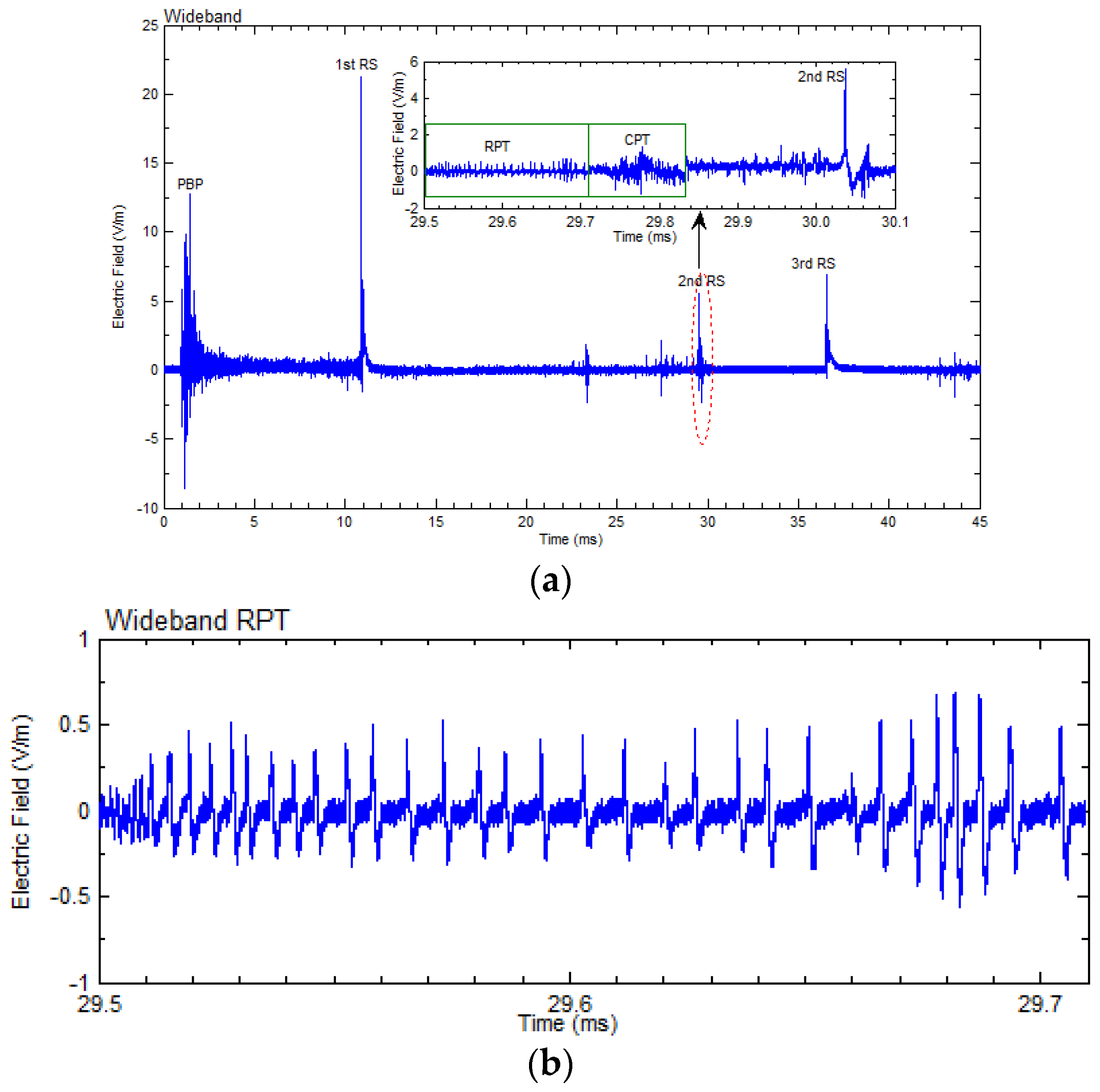
Pulses in the RPT occur at quite regular time intervals. Each pulse in the RPT begins with a fast large-amplitude portion, followed by a small and slowly varying overshoot. However, in some pulses, the opposite overshoot is not that pronounced. If we consider any pulse with an opposite overshoot to be bipolar, then almost all the pulses we observed in the present study can be categorized as bipolar. However, in a study conducted by Kolmasova and Santolik [
10], each individual pulse is considered to be unipolar if the immediately following overshoot of the opposite polarity does not exceed one-half of the peak amplitude of the original’s pulse. If we use this criterion, then most of the individual pulses in the RPT should be categorized as unipolar. In
Figure 2b an RPT is shown which is an expansion from
Figure 2a. Note that the polarity of the pulses is negative here.
As described in
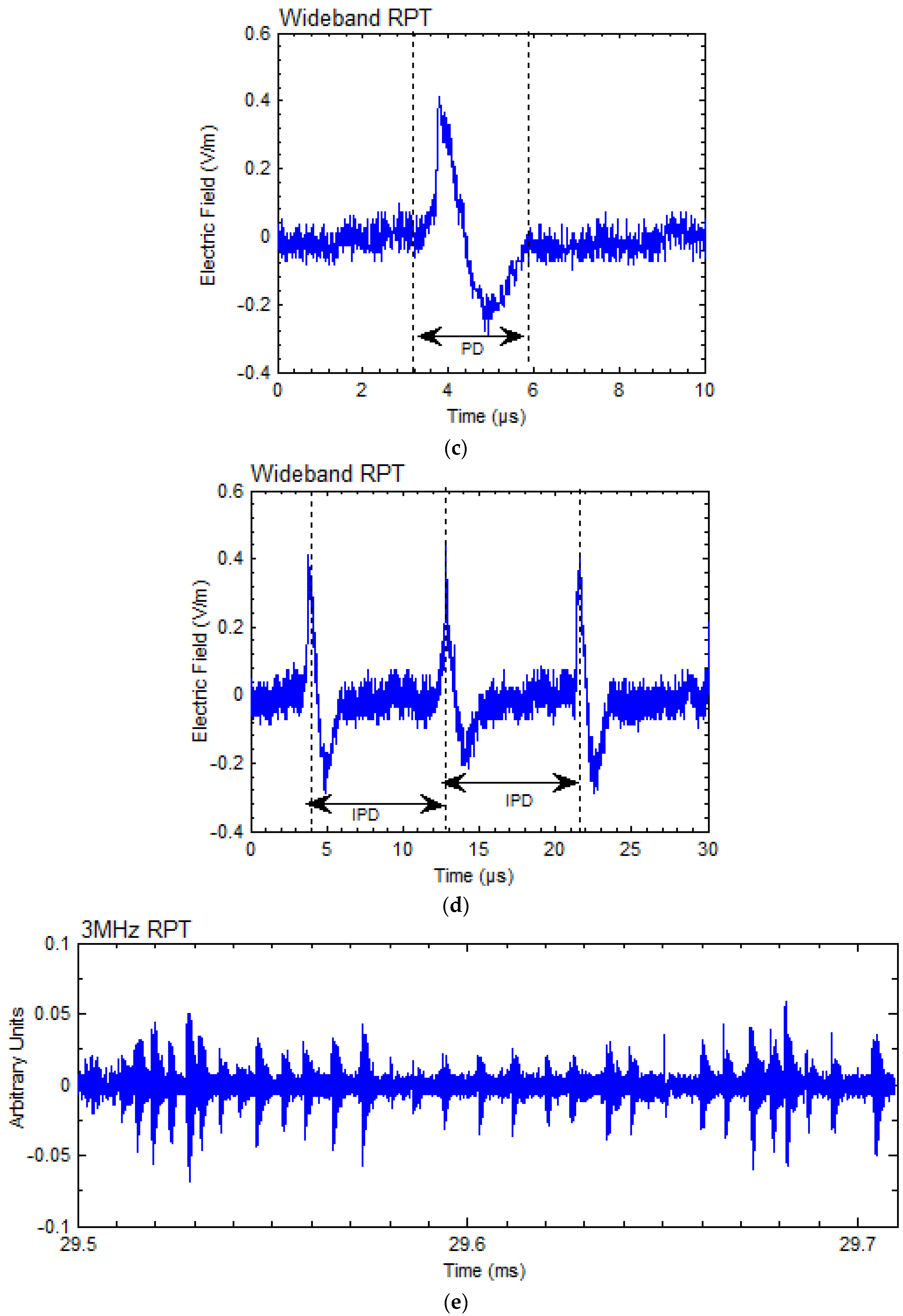
Section 2.2, there were a total of 42 distinct RPTs and the total number of individual pulses in these regular pulse trains was 800. On average, each RPT had about 22 pulses. The individual pulse duration (PD) has an arithmetic mean and standard deviation of about 2 ± 1.0 µs and one typical individual pulse is shown in
Figure 2c, where the PD also is marked. A sequence of pulses normally persists for 23–98 µs with an arithmetic mean and standard deviation of inter-pulse duration (IPD) of about 5 ± 1.3 µs. The IPD is the time duration between the maximum amplitude of two consecutive pulses in the train as shown in
Figure 2d.
As mentioned in
Section 2.2, all RPTs took place in between return strokes and the distribution of these trains was following: 20 distinct RPTs were located between the first and the second RS, 16 distinct RPTs were located between the second and the third RS, and 6 distinct RPTs were located between the third and the fourth RS. The amplitude of the pulses in the RPTs were calculated as a fraction of the following return stroke amplitude. The average electric field amplitude of pulses in the RPT was about one-fifth of the electric field peak of the return stroke, and this ratio varied from 0.1 to 0.4.
All values presented here regarding the parameters of PD and IPD agreed with the values found by Krider et al. [
1] but the values for the total duration of the pulse trains in our case were much lower than that of Krider et al. This can be explained by the fact that the values of the inter-stroke interval for temperate regions (Uppsala) are shorter than that for subtropical regions such as Florida and Arizona [
7].
3.2. Characteristics of the Chaotic Pulse Train (CPT)
There were a total of 1120 individual pulses in those 40 distinct CPTs found in this study. Each distinct CPT had about 28 pulses on average.
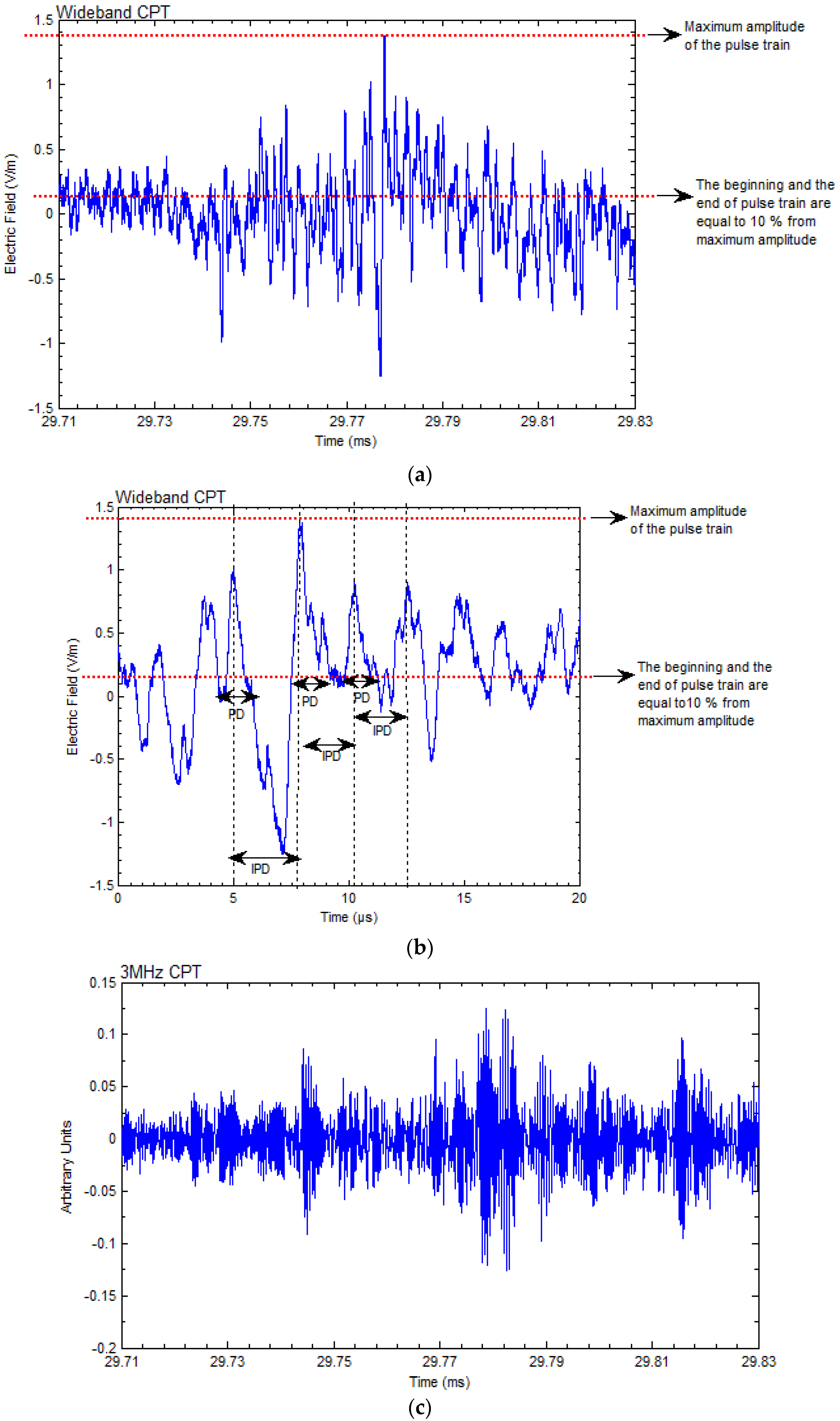
Figure 3a shows an example of CPT which is an expansion of the CPT in
Figure 2a. Because of their chaotic behavior, especially with regard to their amplitudes, pinpointing the exact beginning and end of each pulse in the CPT with good precision is difficult. The total duration (TD) of the CPT is estimated using the criterion adopted by Gomes et al. [
6]. According to this criterion, TD is the time duration between the regions of pulse activity at the start and end of the pulse train where the pulse amplitude is equal to 10% of the maximum amplitude in the CPT. In several cases where the noise level was high, we had to increase this limiting value to 20%. In our study, the observed duration, TD, of the CPTs varied from 20 to 120 µs. We estimated the TD, PD and IPD manually with an estimated uncertainty of about ±0.5 µs. Pulse duration (PD) is the width of an individual pulse when the amplitude at the start and end of the individual pulse is equal to 10% of the maximum amplitude in the CPT. The width of each pulse or its duration (PD) varied within the range of 0.5 to 13 µs with an arithmetic mean and standard deviation of about 4 and 3 µs, respectively. The inter-pulse duration (IPD) is the time duration between the maximum amplitude of two consecutive pulses in the train. The IPD varied within the range from 2 to 13 µs with an arithmetic mean and standard deviation of about 8 and 5 µs, respectively. In
Figure 3b which is an expansion of
Figure 3a, PD and IPD are shown.
As mentioned in
Section 2.2, all CPTs took place in between return strokes and the distribution of these trains was following: 20 distinct CPTs were located between the first and the second RS, 14 distinct CPTs were located between the second and the third RS, and 6 distinct CPTs were located between the third and the fourth RS. As for the amplitudes, sometimes pulses with the largest amplitudes occur immediately after the initiation of the chaotic pulse train, and in some cases, the occurrence of the largest peak happens either in the middle and/or at the end of the chaotic pulse train. The arithmetic mean and standard deviation of the ratio of the maximum amplitude of the pulses to the following return stroke peak were 0.4 ± 0.3.
A comparison of the pulse characteristics found in our study to Gomes et al. [
6] shows a good agreement but the total train duration is not comparable due to the fact that Gomes et al. analyzed and presented data from three different geographical regions together, namely from Sweden, Denmark and Sri Lanka.
3.4. Numerical Analysis: Construction of a CPT through the Numerical Superposition of RPTs
The similarity in the width of individual pulses in both regular pulse trains and chaotic pulse trains and the occurrence of regular pulse trains at the start, in the middle, or at the end of chaotic pulse trains suggested to us the hypothesis that these chaotic pulses are probably created by the superposition of several regular pulse bursts at random times. This is a reasonable physical scenario because during lightning flashes, there could be instances where several dart or dart-stepped leaders, like discharge processes, are simultaneously active in the cloud. Each dart-stepped like leader produces an RPT, and the sum of the signals from all the dart-stepped-like leaders will appear as a CPT. In this section, we will demonstrate this by superimposing RPTs numerically. We will also show that the CPTs constructed in this manner also have Fourier spectrums similar to the ones estimated from the measured CPTs.
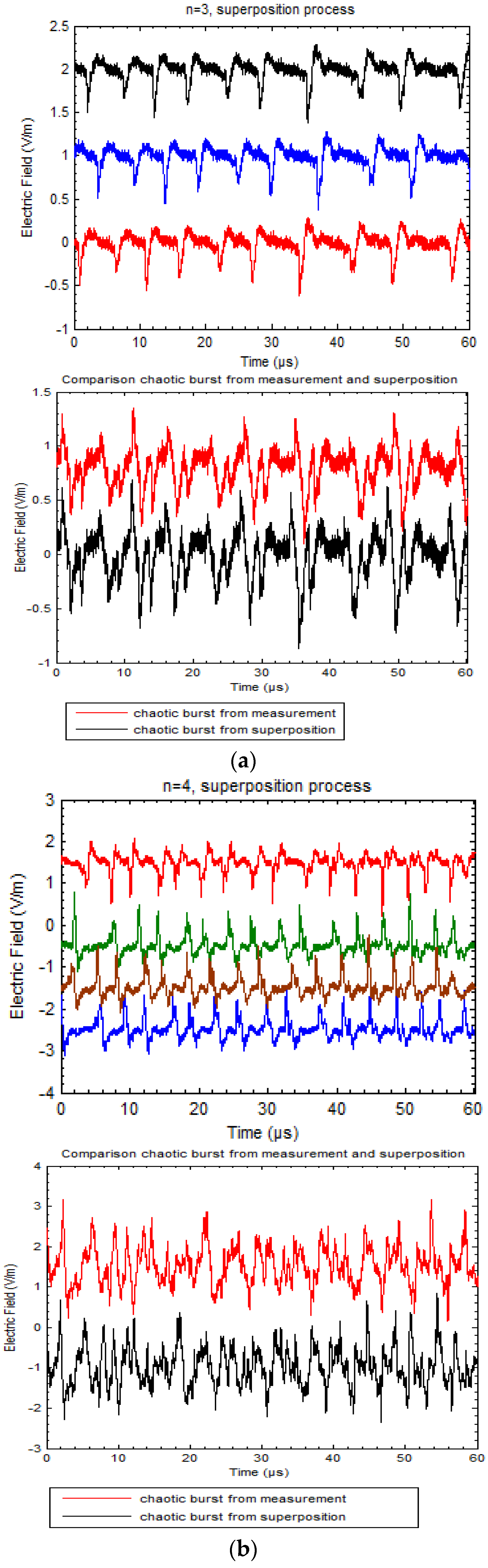
To realize this, out of 42 distinct RPTs we chose one RPT randomly to start with. After selecting a 15- to 60-µs-long section, we took another section from the same RPT with the same length but this time the start of the new section was shifted in time to either direction with 2–5 µs compared to the previous section. In the case of category 3 (RPT–CPT–RPT) where two distinct RPTs were present, sometimes we chose sections of RPTs from both RPTs and sometimes from only one distinct RPT. Then we made a superposition of these two sections. The simulated signal was then compared to the measured CPT belonging to the corresponding train. The comparison was based on their erratic behaviour and the temporal characteristics. This procedure was repeated as a trial and error method. Number of sections that were superimposed, duration of the train section and the position in time of the chosen sections were changed until the best combination was found that corresponded the measured CPT satisfactorily. In
Figure 4a,b the results of our numerical simulation are shown, indicating the best combinations with three (
Figure 4a) and four RPTs (
Figure 4b) and with the 60-µs-long section.
In the numerical superposition, we tried superimposing either the RPT of the same polarity or RPTs with mixed polarities (i.e., adding both positive and negative RPTs to create CPTs). Both procedures gave rise to chaotic-type pulse bursts. The reason we tried constructing a CPT with mixed polarity was because our records showed that we occasionally observed the polarity of pulses in the RPTs changing their polarities. In other words, the RPT may start with pulses of one polarity and then change pulses toward the end of the polarity. This showed us that in some situations it is possible for an RPT of one polarity to interact with an RPT of the opposite polarity in creation of CPTs.
Interestingly, the resulting pulse trains have all the characteristics similar to those observed in chaotic pulse trains. The similarity of the simulated CPT to the ones measured strongly suggests that these pulse trains are created by a series of dart-stepped leader like discharges propagating simultaneously in the cloud.
Since, according to our suggestion, the chaotic pulse burst is a superposition of several regular pulse bursts, the HF associated with the chaotic pulse burst can be treated as the sum of the HF radiation associated with regular pulse bursts. When different HF radiation pulses overlap, depending on their phases, sometimes the resulting amplitude is smaller than that of the RPT, and sometimes it is larger. This means that the peak amplitudes of the HF radiation pulses from chaotic pulse trains will be smaller than that of an RPT in some cases, and it could be larger in other cases.
Figure 2e and
Figure 3c show several examples of HF radiation associated with the RPT and the CPT.
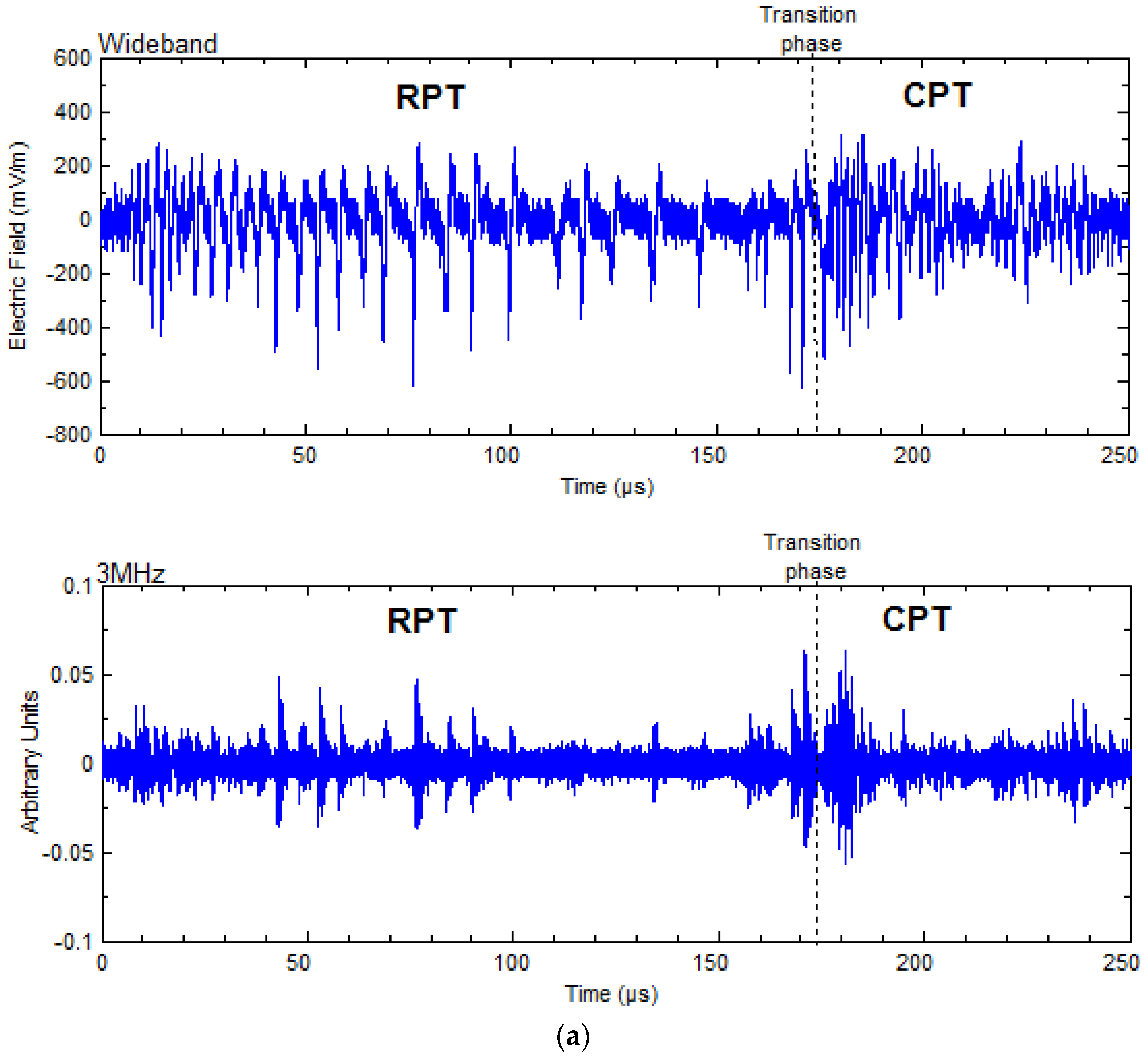
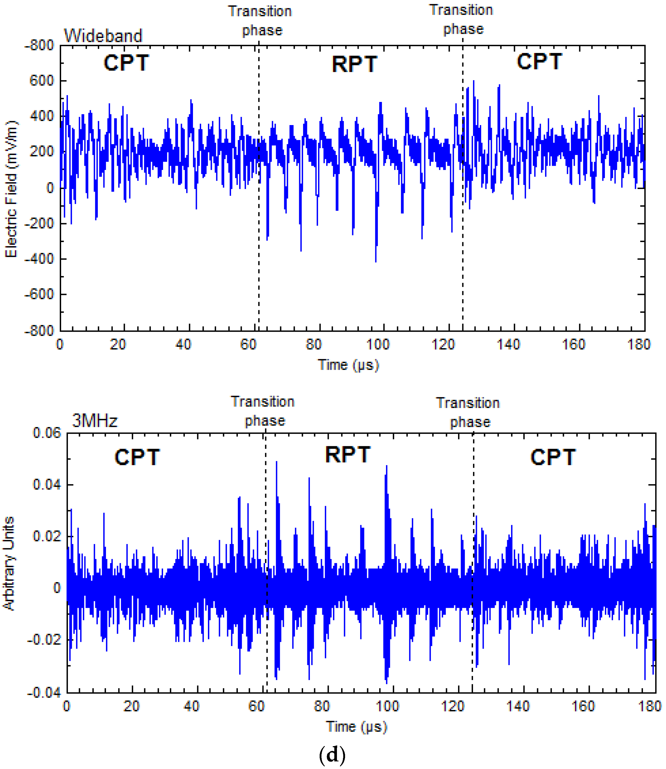
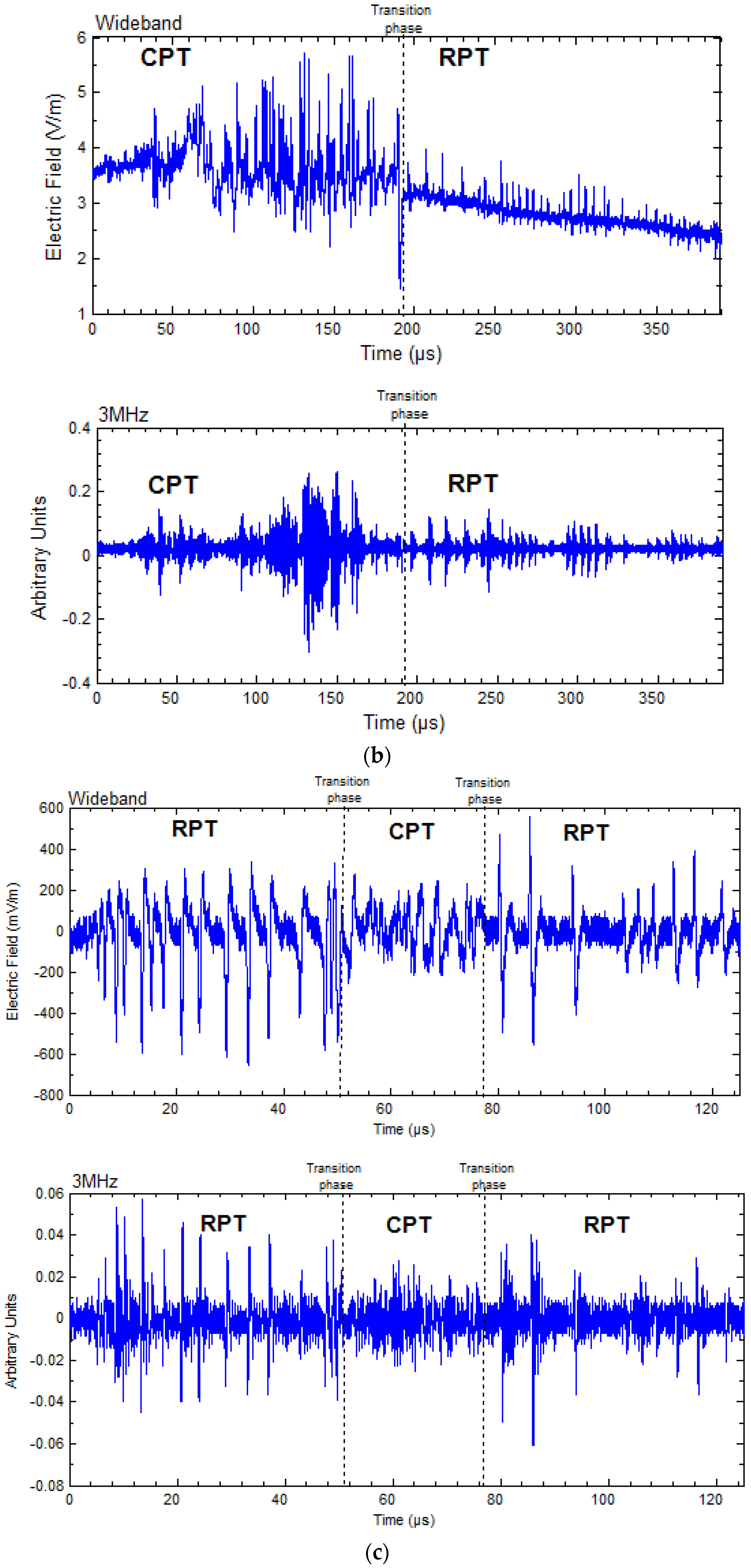
Figure 1b shows the HF radiation associated with a CPT that ended as an RPT. Observe that the amplitude of the HF radiation associated with the regular pulse train is less than the amplitude of the HF radiation associated with the chaotic pulse train. However,
Figure 1c,d shows that the amplitude of the HF radiation associated with an RPT is larger than the amplitude of the HF radiation associated with a CPT. In these cases, one can see the occurrence where the CPT is in the middle of an RPT and the RPT is in the middle of a CPT. The different trends of the amplitude of HF for a CPT and an RPT in some cases are due to destructive and constructive interference. The sum of amplitudes of several RPTs can be less than the amplitudes of all original RPTs, or less than the amplitudes of only a few of the original RPTs but higher than the amplitudes of the remaining original RPTs, or the sum of amplitudes of several RPTs can even be zero because of destructive interference. Meanwhile, when the sum of amplitudes of several RPTs lines up, there is constructive interference. This one can immediately be seen from the recorded data shown in
Figure 1a–d.
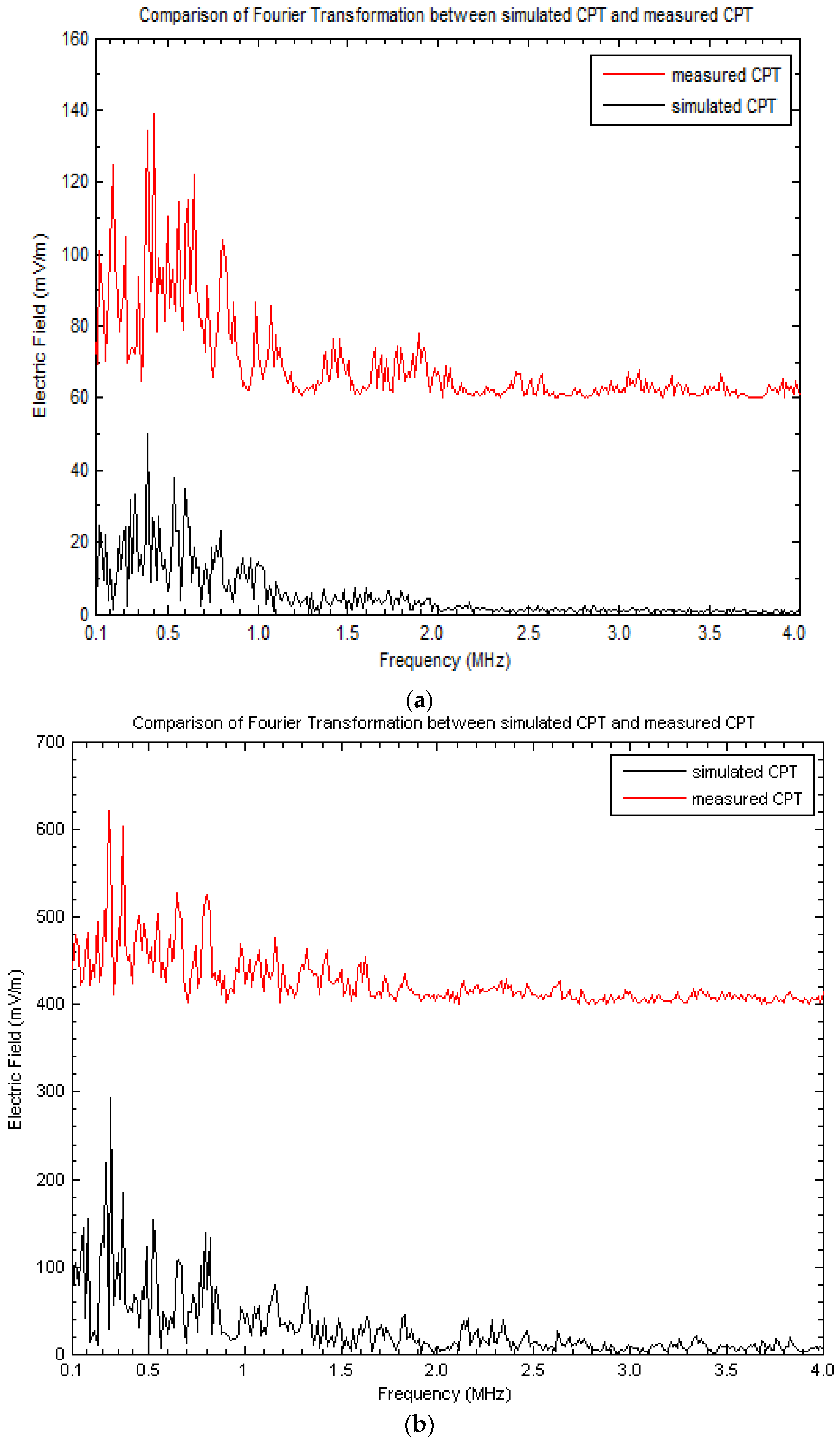
We also analysed the Fourier spectrum of the measured CPT and compared the results with the ones obtained from the simulated CPT. The results of the comparison are shown in
Figure 5a,b. Note that the Fourier spectrums of constructed and measured CPTs are almost identical, and they have a peak around 200 kHz. This similarity of the Fourier spectrums also suggests the common origin of RPTs and CPTs.


 and
and 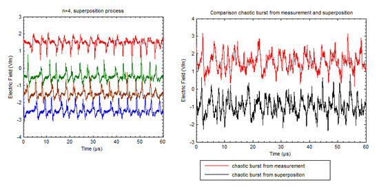