Observations of a Cold Front at High Spatiotemporal Resolution Using an X-Band Phased Array Imaging Radar

Abstract

While the vertical structure of cold fronts has been studied using various methods, previous research has shown that traditional methods of observing meteorological phenomena (such as pencil-beam radars in PPI/volumetric mode) are not well-suited for resolving small-scale cold front phenomena, due to relatively low spatiotemporal resolution. Additionally, non-simultaneous elevation sampling within a vertical cross-section can lead to errors in analysis, as differential vertical advection cannot be distinguished from temporal evolution. In this study, a cold front from 19 September 2015 is analyzed using the Atmospheric Imaging Radar (AIR). The AIR transmits a 20-degree fan beam in elevation, and digital beamforming is used on receive to generate simultaneous receive beams. This mobile, X-band, phased-array radar offers temporal sampling on the order of 1 s (while in RHI mode), range sampling of 30 m (37.5 m native resolution), and continuous, arbitrarily oversampled data in the vertical dimension. Here, 0.5-degree sampling is used in elevation (1-degree native resolution). This study is the first in which a cold front has been studied via imaging radar. The ability of the AIR to obtain simultaneous RHIs at high temporal sampling rates without mechanical steering allows for analysis of features such as Kelvin-Helmholtz instabilities and feeder flow.

1. Introduction

Study of the vertical structure of cold fronts dates back over 40 years, during which time primary interest has been placed on the impact of cold fronts on convection initiation (CI) [1,2]. Later studies have shown that in addition to the presence of CI along the leading edge of the front, waves in the cold front wake may be responsible for CI well after the front has passed [3,4]. More recently, focus has shifted to smaller scale features and, when the observation method allows, their evolution in time [5,6,7,8,9,10]. As seen with applications to gust front detection, radar systems that operate in plan position indicator (PPI) mode do not offer sufficient temporal resolution along a given radial to observe the evolution of small-scale features in the vertical dimension. This lack of knowledge regarding the vertical structure of a cold front and its evolution in time serves as the primary motivation for this study; the methods used allow for cold front analysis that would not be possible via traditional scanning radars in PPI/volumetric mode.

In addition to cold fronts, significant research over the past 30 years has been performed on the prediction and detection of gust fronts, with a focus on detection from an aviation safety perspective [11,12,13]. In the wake of multiple aircraft crashes during the early-to-mid 1980s, the Federal Aviation Administration (FAA) commissioned an investigation into wind shear and gust front detection. Ultimately, the decision was made to fund two wind shear detection methods: the Low-Level Wind Shear Alert System (LLWAS) and the Terminal Doppler Weather Radar (TDWR) [14]. In addition to these two systems, research has been undertaken to provide algorithm-based wind shear and gust front detection, culminating in algorithms such as the Integrated Terminal Weather System (ITWS), Gust Front Detection Algorithm (GFDA), Advanced Gust Front Algorithm (AGFA), and Machine Intelligent Gust Front Algorithm (MIGFA) [12,15,16].

It should be noted, however, that some aspects of gust front dynamics do not apply to cold fronts. Along-front flow and turbulent mixing behind the leading edge of the cold front imply that cold front propagation cannot be modeled in the same manner as density currents [5,7,17,18,19]. However, many features of gust fronts are also seen in cold fronts [6]. Cold air behind the leading edge (nose) is enclosed by a cold front envelope, with turbulent mixing present behind the cold front head. In the wake of the front, multiple trailing surges are typically present, with strong turbulent mixing occurring.

Previous studies of cold front and gust front structure have utilized a wide variety of methods in order to improve overall scientific understanding. Some of these methods include use of radio towers and surface mesonetworks [1,2,20], aircraft in situ observations [21], wind profilers [4], airborne radar passes [5,6,9], ground-based radar in PPI/volumetric mode [11,13,22], vertically pointing radar [23], ground-based lidar [10], or a combination of methods, such as in a field campaign [3,7,8,19,24,25,26]. Additionally, laboratory experiments [27,28,29], theoretical studies [30,31], and computer simulations [17,32,33,34] have been undertaken in order to improve understanding of atmospheric dynamics of cold fronts and gust fronts. In particular, previous research has attempted to explain the manner in which various velocity profiles in phenomena similar to surface-based cold fronts achieve and maintain their instability [30,31]. In a stably stratified layer with an upper shear layer and lower boundary present (such as in a surface-based cold front), it has been shown that gravity waves can be naturally amplified via overreflection (i.e., reflected amplitude is greater than the incident amplitude) by the upper shear layer [31,35]. This, combined with a total reflection at the lower boundary, leads to a situation whereby the gravity wave continues to grow, with vertical oscillations between the upper and lower boundaries. A proof and discussion of this phenomenon can be found in [36].

While many of these studies provide significant insight into the structure of cold fronts and gust fronts, none of the previously conducted studies have used radar at sufficiently high spatial and temporal resolution in order to observe the evolution of small-scale features and their interaction. It is this void in the current body of research that this study aims to fill. By using the Atmospheric Imaging Radar (AIR) in a range-height indicator (RHI) mode through a cold front, radar data are obtained with high spatial sampling (native resolution of 1° in elevation and 37.5 m in range, oversampled to 0.5° in elevation and 30 m in range) and temporal sampling (on the order of 1 s), with continuous vertical coverage. In this mode, instead of scanning mechanically in azimuth, the AIR collected data along a single radial without any mechanical movement. Although it is possible to use an RHI scanning strategy with a pencil-beam radar, this results in the inability to alter temporal sampling after the data are collected, as well as decreased temporal resolution due to the time necessary to scan in elevation. The ability to alter temporal sampling during the processing phase is important, as it allows for decisions regarding data quality to be made after the data are collected. Using this scanning configuration, features such as Kelvin-Helmholtz instabilities (KHIs) were clearly observed. The presence of KHIs has been noted in previous work [5,6,9,17,27,37,38], but the initiation, formation, growth, and decay of KHIs in the atmosphere has sparsely been observed, especially at sufficiently high spatiotemporal resolution. In one study, a lidar observed KHIs while sampling an approaching cold front [10]. However, because the lidar was operating in an interleaved PPI/RHI pattern, temporal resolution for an RHI was still on the order of 30 s between successive RHI scans.

In the case of KHIs, formation can be predicted by estimation of the Richardson number (Ri). Richardson number, a dimensionless number used to quantify the ratio between buoyancy and wind shear, is given by

$$\mathrm{Ri}=\frac{g\Delta \theta }{\theta \Delta z_1}{\left(\frac{\Delta z_2}{\Delta v}\right)}^2$$

(1)

where g is gravitational acceleration, θ is the potential temperature in degrees Kelvin (K), $\frac{\Delta \theta }{\Delta z_1}$ is the local vertical potential temperature gradient, and $\frac{\Delta z_2}{\Delta v}$ is the inverse of the local vertical wind shear. Two distinct values of height differences ($\Delta z_1$ and $\Delta z_2$) are used because of inconsistent vertical sampling between the method of data collection for velocities (AIR) and data point spacing for thermodynamic data; this will be discussed further in later sections. If potential temperature and radial velocity were sampled at identical locations for the entire vertical extent of the analysis, then $\Delta z_1=\Delta z_2$. High Richardson numbers ($\mathrm{Ri}>1$) indicate that buoyancy plays a much larger role in the flow than wind shear, whereas low Richardson numbers ($\mathrm{Ri}<1$) imply that wind shear is the dominant term [36]. Previous studies have shown that KHI formation and sustenance is dependent upon Richardson number, with $\mathrm{Ri}<0.25$ required for KHI formation, and $\mathrm{Ri}<1$ required for KHI sustenance [39,40,41]. In an intuitive sense, a highly stable layer ($\mathrm{Ri}>1$) will suppress vertical motion, making KHI formation less favorable. In the absence of thermodynamic data, KHI characteristics can be used as a proxy for predicting Richardson number, in the sense that there exists a strong correlation between s (defined as the KHI ratio, or billow height divided by billow spacing) and Richardson number, with larger Richardson numbers corresponding to lower s values [37]. Conversely, if the Richardson number is known, an estimate of KHI spacing can be made, assuming that the KHI roughly spans the height of the boundary layer.

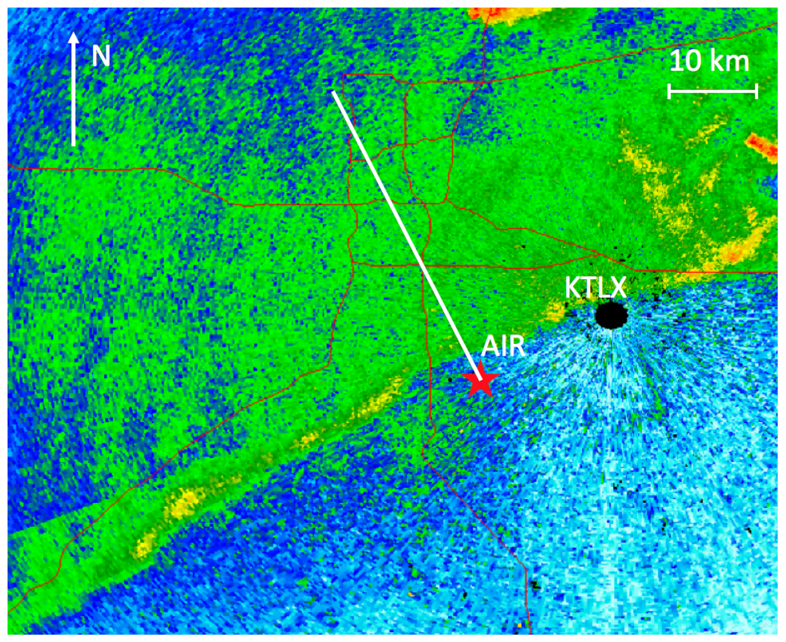
2. Data Collection and Methods

This study is primarily focused on observations of a cold front which passed through central Oklahoma between 0130 UTC and 0400 UTC on 19 September 2015. The AIR deployed on the north side of Norman, Oklahoma at 0215 UTC, and began collecting data at 0226 UTC. During the scan, the AIR did not rotate in azimuth; instead, data were collected along one radial, allowing for maximum temporal resolution and added flexibility of changing temporal sampling during the processing phase. A diagram showing a low-elevation PPI from a local NEXRAD (KTLX), the AIR location, and the AIR scanning radial is shown in Figure 1.

For this case, reliable thermodynamic data in close proximity are unavailable, so Richardson number estimation must be derived via a proxy method. Three methods of Richardson number estimation have been used in this study: first, spatially and temporally displaced sounding data were used as an estimate for a local thermodynamic profile. These data were taken behind the leading edge of the cold front as it passed through northern Oklahoma earlier in the day, and should serve as a somewhat-reliable estimate of the vertical thermodynamic profile. Second, Rapid Refresh (RAP) model output data were used as an estimate of the vertical thermodynamic profile near the scanning location [42]. The overall trend of potential temperature in the vertical dimension via the RAP model matches the overall pattern shown by the displaced sounding data, seen in Figure 2. Finally, the third method of Richardson number estimation will make use of previous studies’ laboratory findings which relate KHI characteristics to Richardson number [37].

In recent years, phased-array weather radar systems have become increasingly commonplace, as attention has been drawn to advantages gained by use of beam multiplexing and agile beam steering [43,44,45,46,47]. This study makes use of the AIR, an X-band phased-array imaging radar designed and built by faculty, staff, and students at the University of Oklahoma Advanced Radar Research Center (OU ARRC) [48]. Because the AIR is an imaging radar, a fan beam is transmitted in elevation, with each of the 36 elements recording a stream of I/Q data on receive (32 elements were used in this case). The reduction in the number of elements in this case has a slight effect on the native elevation resolution on receive (resolution changes from 1° to 1.1°). However, this does not significantly affect the analysis from this case. The 3-dB transmit beamwidth of the AIR is 20° in elevation and 1° in azimuth; this beam configuration is typically referred to as a fan beam [48]. The use of fan beams in imaging radars allows for data to be simultaneously recorded for multiple locations in the scanning domain. Digital beamforming is performed in order to generate beams in elevation. To mitigate ground clutter effects, Capon’s method (adaptive beamforming) has been used [49,50], although other ground clutter mitigation methods have also achieved success [51,52,53].

The transmit beam of the AIR can be steered mechanically in azimuth via a rotating pedestal to create its volume coverage pattern (VCP). For this study, the beam was not steered in azimuth, in order to obtain frequent updates along a given radial. In this configuration, any number of pulses can be combined in one RHI. Therefore, the decision has been made to refer to the chosen RHI update time as ‘temporal sampling’ rather than ‘temporal resolution’. In this study, temporal sampling of 1.2 s is used. Faster temporal sampling is possible by combining fewer pulses into each RHI. However, reducing the number of independent samples per RHI leads to a decrease in data quality [54]. This effect is especially pronounced in cases where the signal from meteorological echoes is close to the noise floor (i.e., low signal-to-noise ratio, or SNR). It was found that sampling of 1.2 s provides an acceptable balance between temporal update time and data quality.

In order to increase sensitivity, a ‘high sensitivity’ mode was designed for the AIR based on the method described in [55]. As opposed to the standard 5.25 $\mathsf{\mu }$s waveform used by the AIR for studies of severe local storms [56], a 13.25 $\mathsf{\mu }$s pulse was developed for use on transmit. This waveform offers an approximate 4 dB gain in SNR. Due to a 2% duty cycle limitation, the PRT was chosen to be 757 $\mathsf{\mu }$s, corresponding to a Nyquist velocity of 10.4 m·s${}^{-1}$. Digital beamforming offers several advantages over more traditional ‘pencil-beam’ radar VCPs, mainly in generating simultaneous RHIs, such that vertical advection is not an issue [47,48,56,57]. Additionally, the AIR offers significant processing flexibility (adjustable temporal sampling and beamforming type for sensitivity and clutter mitigation). These advantages allow for improved analysis of the vertical structure of a cold front.

3. Results

New findings from this research are made possible because of the high spatial and temporal resolution offered by the AIR. The ability to observe the evolution and interaction of small-scale features behind the leading edge of a cold front has revealed several features that had sparsely been analyzed or noted in previous studies. In particular, the presence, evolution, and decay of KHIs is observed throughout the majority of the scan. While KHI evolution can be properly observed with slower update times than those in this study, other observed features such as rear-to-front mass transport (feeder flow) cutoff and reestablishment do require temporal resolution on the order of a few seconds [18]. Video S1 in Supplementary Materials shows the approaching cold front, the KHIs, and feeder flow cutoff and reestablishment.

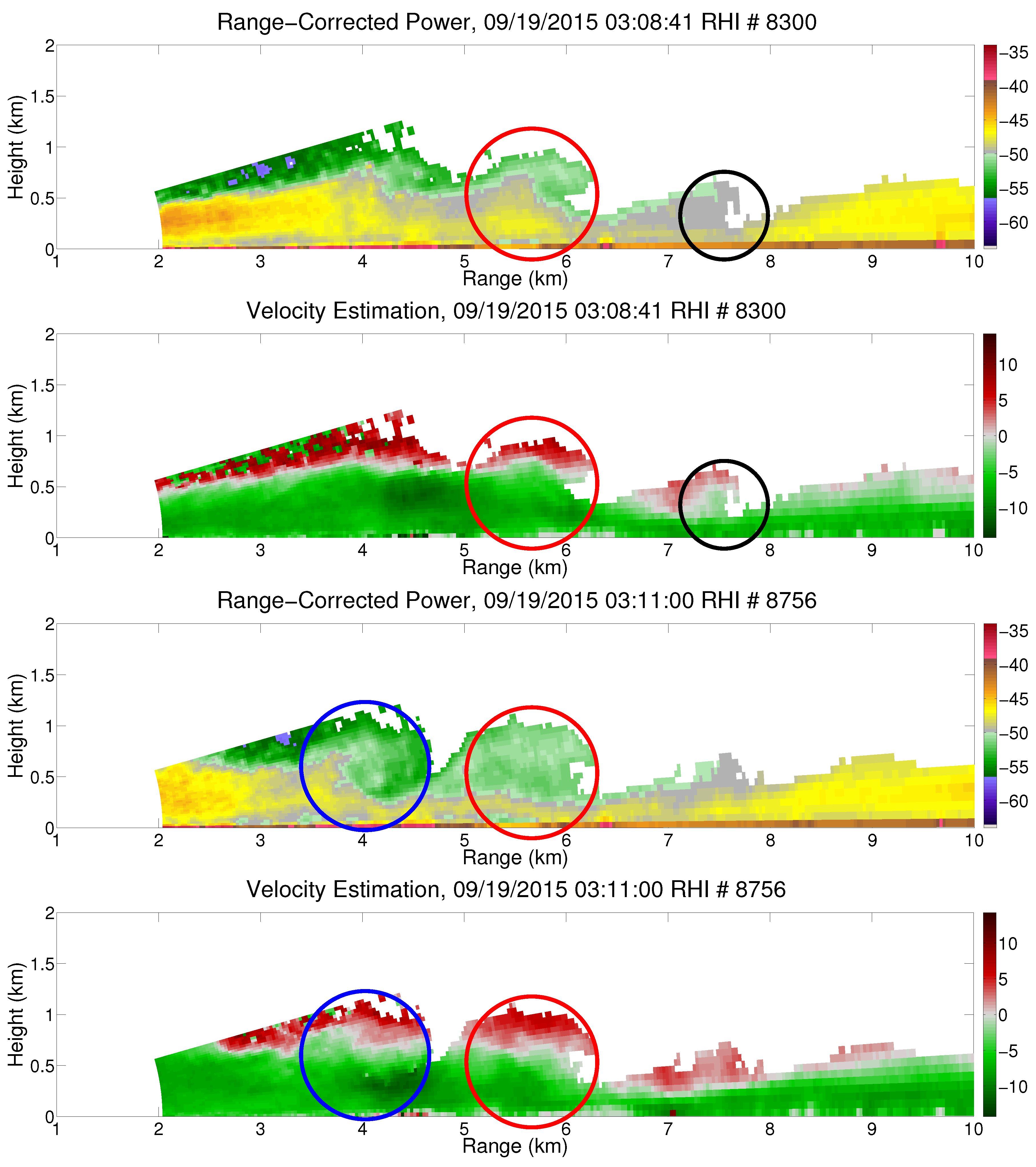
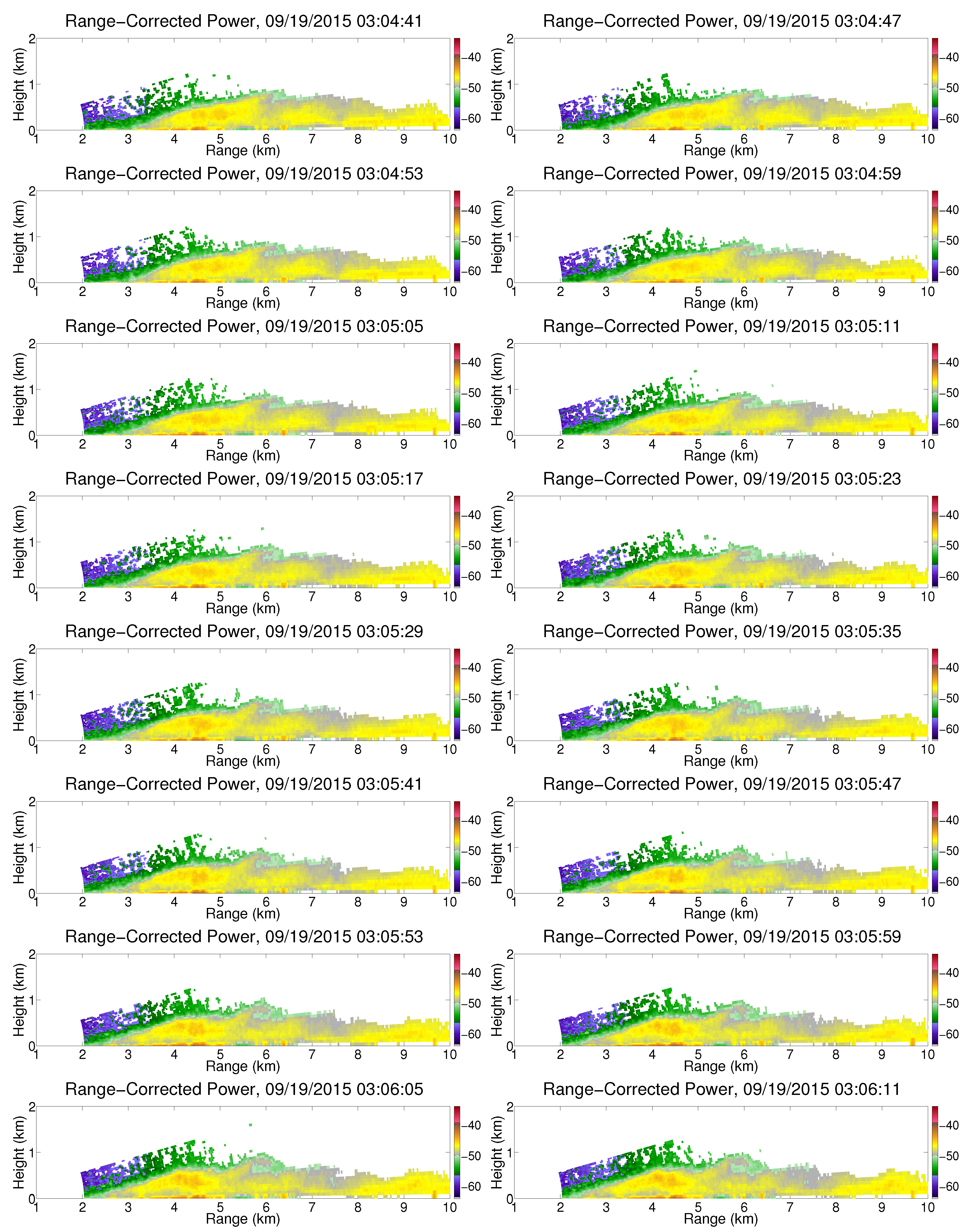
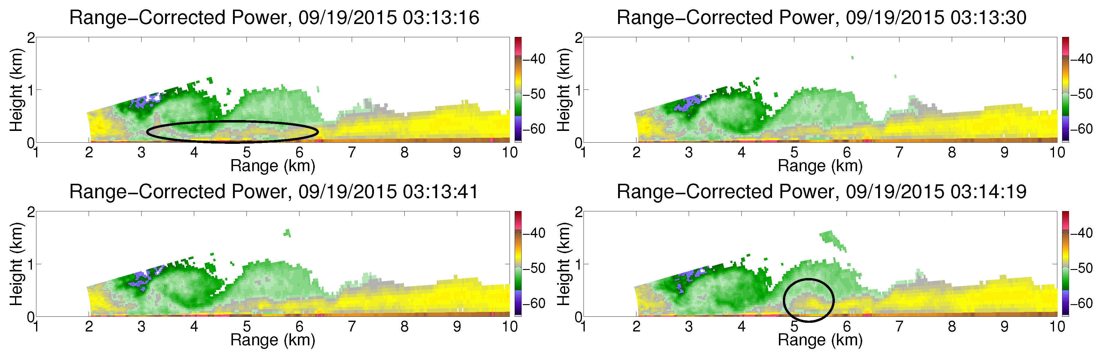
3.1. Kelvin-Helmholtz Instabilities

Multiple instances of KHIs, which are the result of a growing disturbance along a velocity shear interface, are observed. In two instances, the initiation, formation, and growth (and eventual decay via an energy cascade process) of the same KHI is observed, which offers insight into the KHI evolutionary process. Figure 3 shows multiple KHI instances observed in the 19 September 2015 dataset: a decaying KHI is seen in the top panel at 7.5 km in range, a fully mature KHI is seen in both panels at approximately 5.75 km in range, and a newly forming KHI is observed in the bottom panel at 4 km in range.

As the cold front propagates southward, a small protrusion forms across the interface between the two airmasses, and cold air is elevated into the ambient airmass of warmer, southerly winds. Because of the large velocity shear across the interface (0.02–0.04 s${}^{-1}$ based on radial velocity estimates from the AIR), this protrusion grows into a horizontal roll vortex (eventually a KHI) which is observed in power, velocity, and spectrum width. The process by which a protrusion is initially formed is discussed further in later sections. Once a KHI has fully formed, its airflow is entirely cut off from that of the cold front, leading to a significant decrease in propagation speed (overall propagation speed of 0–1 m·s${}^{-1}$).

Although one study has noted that for many atmospheric applications, a velocity shear greater than 0.009 s${}^{-1}$ is sufficient for KHI formation [24], wind shear alone is not sufficient for diagnosing the formation of KHIs in all atmospheric applications, as a vertical thermodynamic profile is necessary to estimate Richardson number.

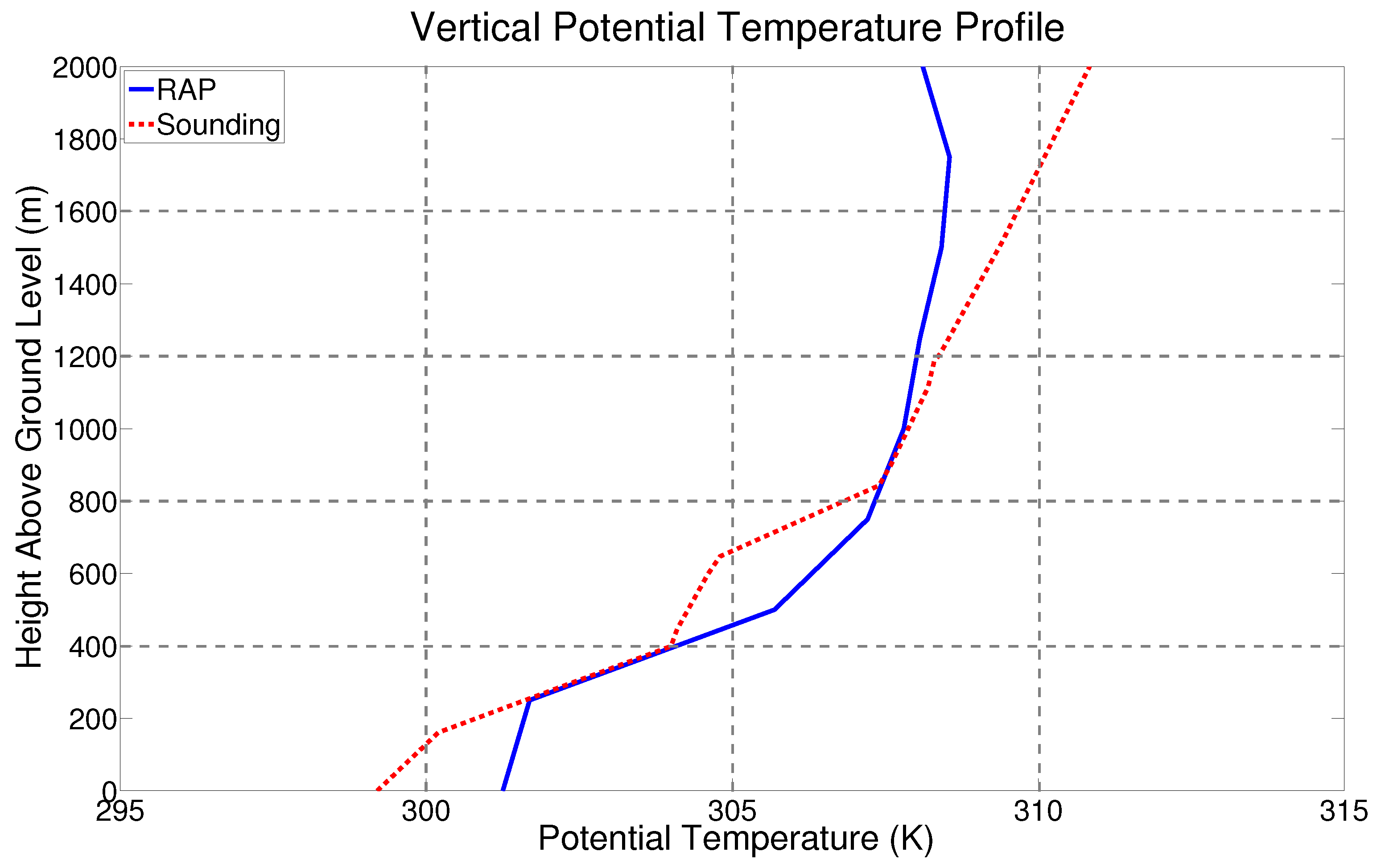
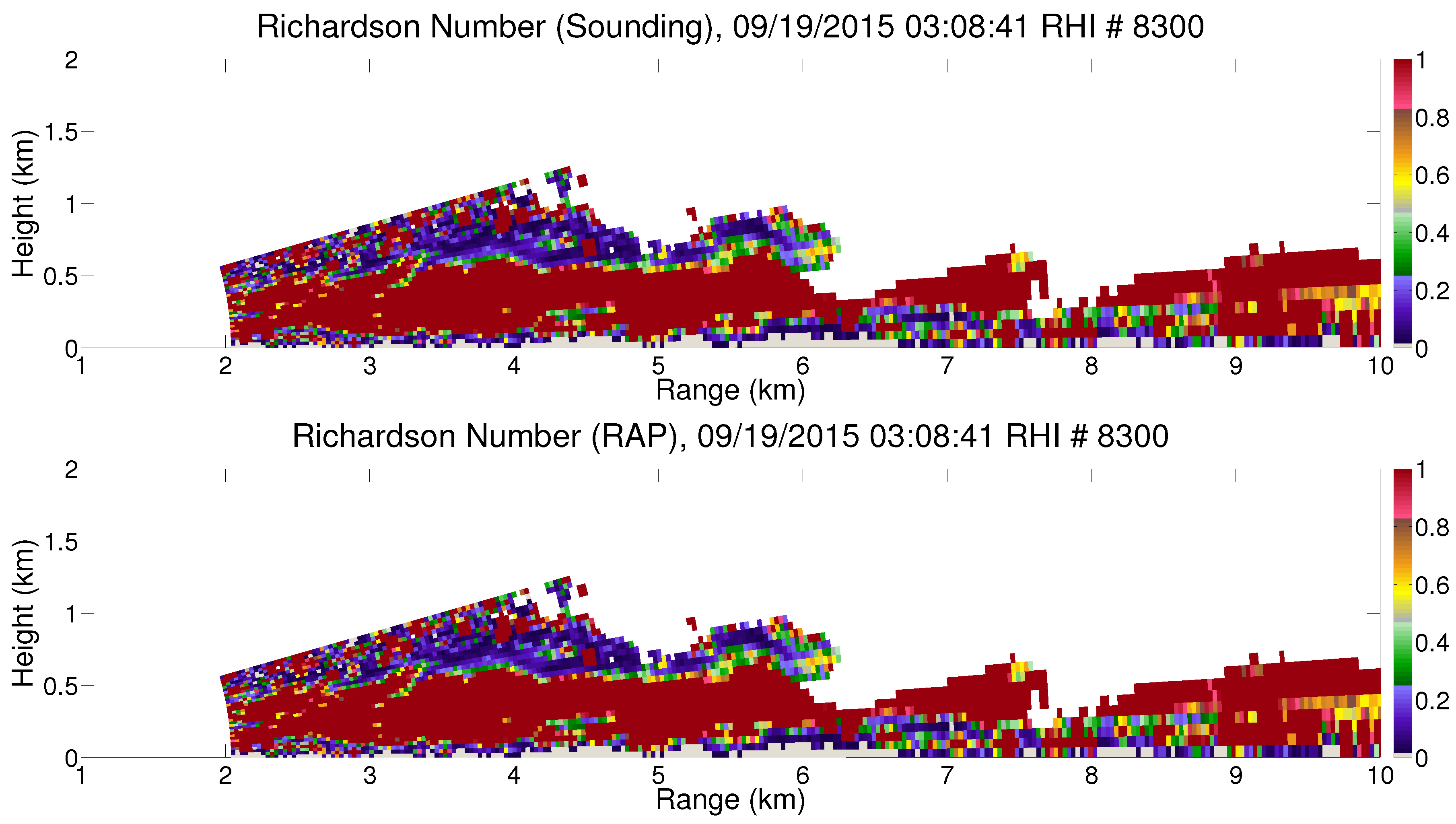
3.2. Richardson Number Estimation

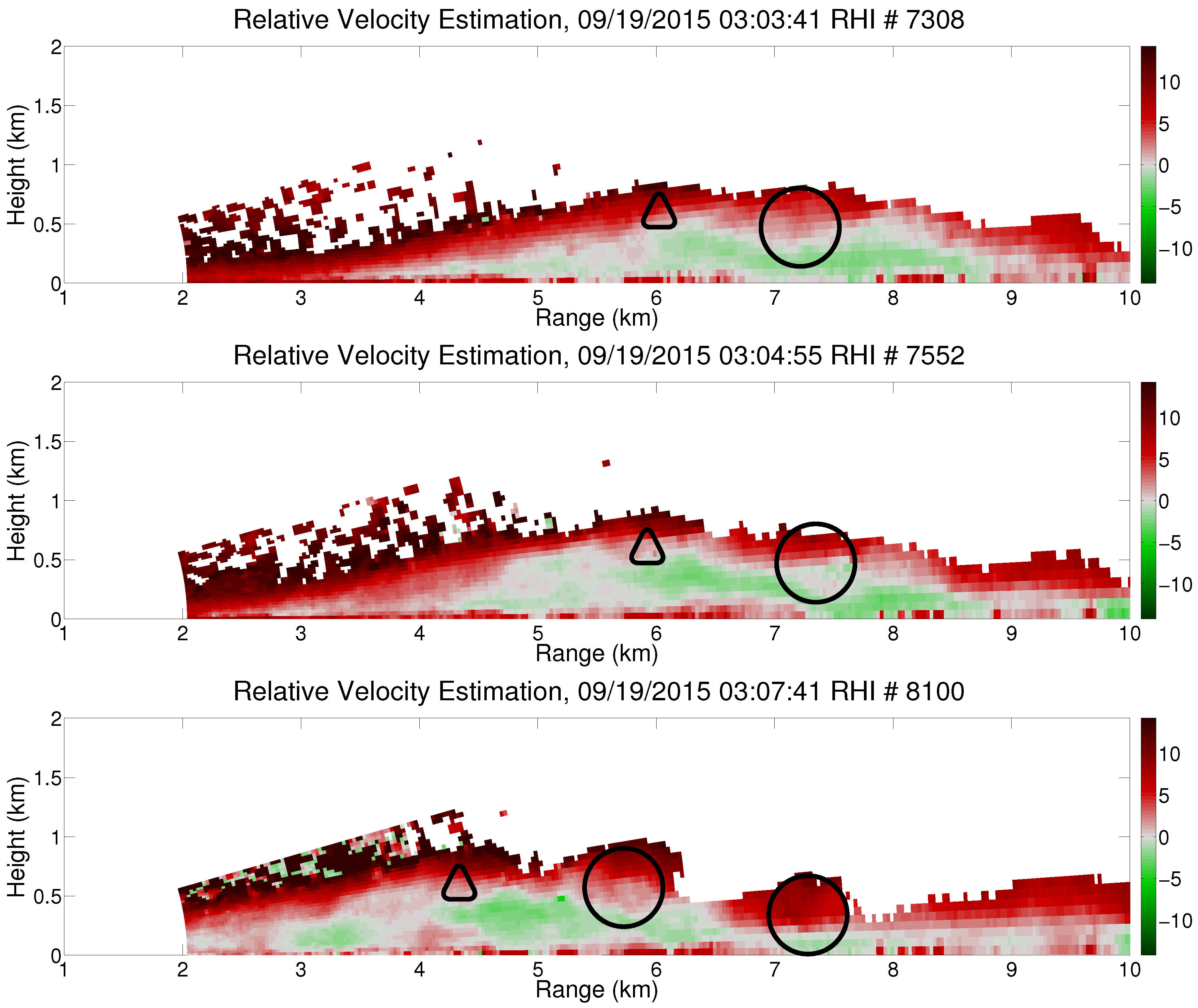
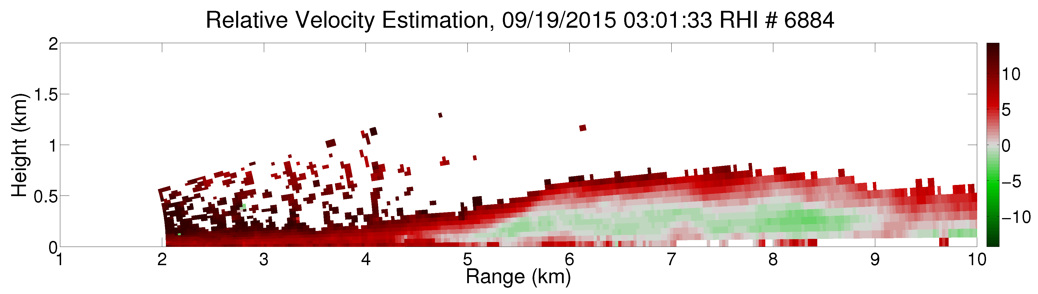
In this case study, in situ thermodynamic data were unavailable. Because the data were collected around 0300 UTC, a sounding from the local site (launched at 0000 UTC) did not provide an accurate depiction of the vertical thermodynamic profile during the scan. As a proxy for in situ thermodynamic data, a sounding from northern Oklahoma, also launched at 0000 UTC, was used. This was done because this sounding (hereinafter referred to as the ‘displaced sounding’) was launched shortly after cold frontal passage, and offers thermodynamic data after cold frontal passage. The thermodynamic profile (potential temperature data shown as the blue line in Figure 2) shows evidence of frontal passage based on (1) northerly wind direction in the lowest 1 km (not shown); and (2) nearly zero lapse rates throughout the lower half of the boundary layer [58]. To obtain another estimate of the vertical thermodynamic profile for Richardson number estimation, vertical thermodynamic data from the RAP model was used. The data used were from the 0300 UTC RAP analysis (dashed red line in Figure 2), with the model sounding taken from a gridpoint close to the scanning location where frontal passage had already occurred. These vertical thermodynamic data were combined with AIR data to estimate Richardson number by using the vertical potential temperature change with height from the sounding and the vertical wind shear from the AIR data.

To produce RHIs depicting Richardson number estimation, the AIR radial velocity data was used as a basis. For each range and elevation combination in the AIR RHI, the potential temperature term in Equation (1) is determined by linear interpolation of the nearest thermodynamic data points above and below the point of interest. The local vertical potential temperature gradient at a point is determined by dividing the difference in potential temperature directly above and below the point of interest by the height between these two reference points. Height estimation of each range and elevation combination is determined by the radar beam height equation [54].

Finally, another method was used for Richardson number estimation based on findings which link KHI characteristics to Ri [37]. This method is unique in that a local thermodynamic profile is not necessary for Richardson number estimation. The Richardson number estimated with this method only requires two inputs: KHI spacing and KHI height. Therefore, no radial velocity or local thermodynamic data are necessary for Ri estimation using this method. Although the original paper uses a laboratory experiment to reach these conclusions, this study will propose a similar link between Richardson number and KHI characteristics.

Using the first two methods of Richardson number estimation (shown in Figure 4), a thin layer of lowered Richardson number along the interface between the two boundaries is observed, primarily due to the vertical shear along this interface. By taking the average Richardson number along this interface for both methods, we observe an average Ri value between 0.13 and 0.22 along the interface. These values were obtained by selecting sample regions along the interface (approximate height of sample region: 100–200 m; approximate length of sample region: 400–500 m), and calculating the average Richardson number value in the sample region. These values are consistent with what could be expected from theory, as Ri must be below 0.25 for KHI formation. Thorpe’s method, however, returns a lower estimate of Richardson number (0.10 to 0.13). The results from all 3 methods are shown in

Table 1. Richardson number estimation using the 3 methods described above. Note that Richardson number estimated using Thorpe’s method is significantly lower than Richardson number estimated by the other two methods.

Richardson Number Estimation Method	Rimin	Rimax
Displaced Sounding	0.13	0.20
RAP Model Output	0.14	0.22
Thorpe 1973 Findings	0.10	0.13

.

While the Richardson number estimates from Thorpe’s method do not align with estimates from the other two methods, this can possibly be explained by differences between flow in an idealized laboratory density current and a cold front in the atmosphere. Additionally, previous research has indicated that a Richardson number between 0.10 and 0.15 should correspond to an s value of 0.15 to 0.40, indicating that the estimate from Thorpe’s method may be valid [59]. However, the relationship between Richardson number and s should hold true for atmospheric applications: as Richardson number increases, s should decrease.

3.3. Feeder Flow

In addition to KHIs, feeder flow was also observed in the 19 September 2015 cold front case. Feeder flow is a relative rear-to-front low-level mass transport, and is typically present behind the leading edge of a density current [18]. This region of faster air transports scatterers towards the nose of the front; this flow results in either a mass buildup at the nose of the boundary, or a ‘rotor circulation’ in which scatterers are lofted up near the nose of the front [7]. While feeder flow is typically present in density currents, not all cold fronts contain a feeder flow [19]. In the case of the 19 September 2015 cold front, feeder flow spanning approximately 100–150 m in height is observed behind the leading edge of the cold front, passing underneath the KHIs. The process in which the feeder flow is severed is shown in Figure 5.

For several minutes, the feeder flow is observed to exist as a thin ribbon in power return. As one of the KHIs (centered at 4 km in range) begins to slowly descend, the feeder flow is confined to the lowest few hundred meters. At 03:13:16 UTC, the feeder flow is fully intact (circled in the top left panel of Figure 5), spanning from 3 km in range to 6 km in range. At 03:13:30 UTC, the feeder flow appears broken in some spots, due to the constriction in height. By 03:13:41 UTC, the feeder flow has been fully disrupted, as the KHI at 4 km in range has further descended to cut off the mass transport. Following this flow cutoff, a buildup of mass appears at 5.25 km in range (circled in the bottom right panel of Figure 5). Over the next 2 min (see Video S1 in Supplementary Materials), this mass buildup diminishes, and feeder flow is reestablished.

The rapidly evolving nature of feeder flow cutoff is an essential motivator of temporal resolution on the order of a few seconds. The feeder flow evolves from being fully intact to being broken in multiple locations in 14 s, and is fully interrupted 11 s later. With slower temporal updates, this phenomenon could not be observed in as much detail, and one would risk not capturing this cutoff event.

4. Discussion

4.1. KHI Initiation & Formation Observations

Presence of a Richardson number below the critical Richardson number (0.25) has been shown to coincide with the formation and sustenance of KHIs [37]. However, for Richardson numbers below this threshold, there is no complete existing theory in the literature which attempts to explain why there is a correlation between Richardson number and the ratio of KHI height to KHI spacing. In the 19 September 2015 case, relative velocity estimates (with respect to the cold front motion) reveal a region of rear-to-front flow behind the leading edge of the cold front. This phenomenon is shown in Figure 6. Because of the RHI scanning configuration, it is not known at this time whether this region of relatively high radial velocity estimates is a jet (with minimal horizontal extent) or a shear layer, spanning a greater distance along the cold front. However, we believe that because KHI initiation should not be limited to this specific cross-section, this phenomenon is most likely present across a wider horizontal extent, which would be most consistent with a shear layer. A PPI scan would be necessary to definitively diagnose the horizontal extent of this region.

In the region of an existing KHI, the relative flow is tilted around the KHI, and on the upstream side is tilted upward (toward the interface) by the KHI. As a result, the shear layer causes a protrusion of air to form along the interface between the two airmasses, approximately 2 km closer to the leading edge of the cold front than the existing KHI. This protrusion is observed to grow into a full-grown KHI; Figure 7 shows an example of a protrusion forming at 5.75 km in range.

As the KHI becomes fully formed, the rear-to-front flow (which was previously tilted upwards towards the interface) is curved around the newly formed KHI, creating a new protrusion further upstream. This protrusion typically appears as a triangular or semicircular shape protruding from an otherwise smooth cold front envelope. This process is observed in the 19 September 2015 case in multiple occurrences, as the formation of a new KHI creates an upstream protrusion, which grows into another KHI. This observation regarding a protrusion being formed via flow tilting is supported by RHIs of both relative velocity and radial convergence (as vertical flow tilting can manifest as convergence in a fixed-location RHI). It should be noted, however, that KHIs are simply formed due to shear instability; the remarks correlating KHI initiation with flow tilting imply only that the protrusion is a source of an initial instability, which then grows into a full KHI due to vertical velocity shear. In this particular case, it appears that the shear layer tilting is related to the KHI spacing, rather than ensuring the formation of KHIs.

Additionally, we believe that this observation fits well with previous theories regarding gravity waves in the wake of a cold front [30,31]. Figure 8 shows an oscillatory motion in the vertical dimension, which appears to be the result of a gravity wave. It can be theorized, then, that the shear layer tilting which occurs simply forces a trough in the oscillation directly underneath an existing KHI. Therefore, it is believed that this proposed KHI spacing mechanism agrees with previous findings and theory. The fact that the wavelength of the shear layer oscillation prior to KHI initiation is shorter than the KHI spacing can be explained by noting that the propagation speed of a KHI is nearly zero. This leads to increased spacing between consecutive KHIs as compared to crest-to-crest spacing in the shear layer prior to KHI initiation.

4.2. Potential Relationship between Richardson Number and KHI Characteristics

We observe that in the 19 September 2015 case, the rear-to-front relative flow plays a vital role in KHI initiation. For this case, shear layer tilting is clearly critical to the placement and spacing of subsequent KHIs. The potential effect of Richardson number on KHI spacing is theorized as follows: once the critical Richardson number condition has been met, additional lowering of Ri will either lead to stronger (i.e., more turbulent) KHIs, or greater overreflection and amplitude growth at the shear boundary. It should be noted, however, that a link between Richardson number and KHI strength and/or overreflection amplitude has not been noted in this particular study, and would require further research to prove definitively. Because the trajectory of the rear-to-front flow follows the KHI, a stronger KHI should induce more shear layer tilting than a weaker KHI. Additionally, greater amplitudes due to greater overreflection should reduce the shear layer oscillation wavelength (and also KHI spacing). In either mechanism, as the shear layer is tilted around a KHI, the protrusion point of additional KHIs is altered, such that a more tilted shear layer leads to closer KHI spacing. If there are no significant changes to KHI height, closer KHI spacing should correspond to a higher s value. An overall correlation between low Richardson number and high s values corresponds well with previous findings [37]. It should again be noted that these findings cannot necessarily be extrapolated as an overarching theory for KHI spacing without further study. Additionally, due to the lack of friction above the planetary boundary layer and the lack of an impermeable lower boundary, there is currently no reason to believe that an identical flow-tilting mechanism should hold true in applications where the role of the surface of the earth and the planetary boundary layer are negligible. Further cases would need to be studied in order to fully assess the applicability of these findings.

4.3. Proposed Future Work

Future work on KHI observations behind quasilinear meteorological features (such as cold fronts and gust fronts) would include obtaining a vertical thermodynamic profile via in situ measurements to improve Richardson number estimation. Use of a polarimetric radar could provide meaningful information regarding scatterer types, assuming the wavelength of the radar is such that meaningful polarimetric information can be extracted for relatively small scatterers. Additionally, more cases should be observed in order to understand the limits to applicability of these findings. The flow-tilting mechanism observed here might not be present in the case of upper-tropospheric Kelvin-Helmholtz clouds, non-surface-based fronts, or even some surface-based cold fronts. Finally, this study provides evidence that future widespread implementation of phased array and/or imaging radar systems could lead to greater predictability of surface-based wind shear and turbulence due to improved spatiotemporal resolution. The applicability to detection algorithms is an important area for future study, which can be achieved through additional observations by the AIR and/or other radar systems.

References

1. Charba, J. Application of Gravity Current Model to Analysis of Squall-Line Gust Front. Mon. Weather Rev. 1974, 102, 140–156. [Google Scholar] [CrossRef]
2. Goff, R.C. Vertical Structure of Thunderstorm Outflows. Mon. Weather Rev. 1976, 134, 1429–1440. [Google Scholar] [CrossRef]
3. Weckwerth, T.M.; Wakimoto, R.M. The Initiation and Organization of Convective Cells atop a Cold-Air Outflow Boundary. Mon. Weather Rev. 1992, 120, 2169–2187. [Google Scholar] [CrossRef]
4. May, P.T. Thermodynamic and Vertical Velocity Structure of Two Gust Fronts Observed with a Wind Profiler/RASS during MCTEX. Mon. Weather Rev. 1999, 127, 1796–1807. [Google Scholar] [CrossRef]
5. Wakimoto, R.M.; Bosart, B.L. Airborne Radar Observations of a Cold Front during FASTEX. Mon. Weather Rev. 2000, 128, 2447–2470. [Google Scholar] [CrossRef]
6. Geerts, B.; Damiani, R.; Haimov, S. Finescale Vertical Structure of a Cold Front as Revealed by an Airborne Doppler Radar. Mon. Weather Rev. 2006, 134, 251–271. [Google Scholar] [CrossRef]
7. Friedrich, K.; Kingsmill, D.E.; Flamant, C.; Murphey, H.V.; Wakimoto, R.M. Kinematic and Moisture Characteristics of a Nonprecipitating Cold Front Observed during IHOP. Part I: Across-Front Structures. Mon. Weather Rev. 2008, 136, 147–172. [Google Scholar] [CrossRef]
8. Friedrich, K.; Kingsmill, D.E.; Flamant, C.; Murphey, H.V.; Wakimoto, R.M. Kinematic and Moisture Characteristics of a Nonprecipitating Cold Front Observed during IHOP. Part II: Alongfront Structures. Mon. Weather Rev. 2008, 136, 3796–3821. [Google Scholar] [CrossRef]
9. Geerts, B.; Miao, Q. Vertically Pointing Airborne Doppler Radar Observations of Kelvin-Helmholtz Billows. Mon. Weather Rev. 2010, 138, 982–986. [Google Scholar] [CrossRef]
10. Mayor, S.D. Observations of Seven Atmospheric Density Current Fronts in Dixon, California. Mon. Weather Rev. 2011, 139, 1338–1351. [Google Scholar] [CrossRef]
11. Klingle, D.L. A Gust Front Case Studies Handbook; ATC Proj. Rep. DOT/FAA/PM-84/15; MIT Lincoln Laboratory: Lexington, MA, USA, 1985. [Google Scholar]
12. Uyeda, H.; Zrnić, D.S. Automatic Detection of Gust Fronts. J. Atmos. Ocean. Technol. 1986, 3, 36–50. [Google Scholar] [CrossRef]
13. Klingle, D.L.; Smith, D.R.; Wolfson, M.M. Gust Front Characteristics as Detected by Doppler Radar. Mon. Weather Rev. 1987, 115, 905–918. [Google Scholar] [CrossRef]
14. Whiton, R.C.; Smith, P.L.; Bigler, S.G.; Wilk, K.E.; Harbuck, A.C. History of Operation Use of Weather Radar by U.S. Weather Services. Part II: Development of Operational Doppler Weather Radars. Weather Forecast. 1998, 13, 244–252. [Google Scholar] [CrossRef]
15. Delanoy, R.L.; Troxel, S.W. Automated Gust Front Detection Using Knowledge-Based Signal Processing. In Proceedings of the IEEE Radar Conference, Lynnfield, MA, USA, 20–22 April 1993.
16. Hermes, L.G.; Witt, A.; Smith, S.D.; Klingle-Wilson, D.; Morris, D.; Stumpf, G.J.; Eilts, M.D. The Gust-Front Detection and Wind-Shift Algorithms for the Terminal Doppler Weather Radar System. J. Atmos. Ocean. Technol. 1993, 10, 693–709. [Google Scholar] [CrossRef]
17. Droegemeier, K.K.; Wilhelmson, R.B. Numerical Simulation of Thunderstorm Outflow Dynamics. Part I: Outflow Sensitivity Experiments and Turbulence Dynamics. J. Atmos. Sci. 1987, 44, 1180–1210. [Google Scholar] [CrossRef]
18. Smith, R.K.; Reeder, M.J. On the Movement and Low-Level Structure of Cold Fronts. Mon. Weather Rev. 1988, 116, 1927–1944. [Google Scholar] [CrossRef]
19. Sinclair, V.A.; Niemelä, S.; Leskinen, M. Structure of a Narrow Cold Front in the Boundary Layer: Observations versus Model Simulation. Mon. Weather Rev. 2012, 140, 2497–2519. [Google Scholar] [CrossRef]
20. Young, G.S.; Johnson, R.H. Meso- and Microscale Features of a Colorado Cold Front. J. Clim. Appl. Meteorol. 1984, 23, 1315–1325. [Google Scholar] [CrossRef]
21. Nielsen, J.W. In Situ Observations of Kelvin-Helmholtz Waves along a Frontal Inversion. J. Atmos. Sci. 1992, 49, 369–386. [Google Scholar] [CrossRef]
22. Wakimoto, R.M. The Life Cycle of Thunderstorm Gust Fronts as Viewed with Doppler Radar and Rawinsonde Data. Mon. Weather Rev. 1982, 110, 1060–1082. [Google Scholar] [CrossRef]
23. Martner, B.E. Vertical Velocities in a Thunderstorm Gust Front and Outflow. J. Appl. Meteorol. 1997, 36, 615–622. [Google Scholar] [CrossRef]
24. Mueller, C.K.; Carbone, R.E. Dynamics of a Thunderstorm Outflow. J. Atmos. Sci. 1987, 44, 1879–1898. [Google Scholar] [CrossRef]
25. Mahoney, W.P., III. Gust Front Characteristics and the Kinematics Associated with Interacting Thunderstorm Outflows. Mon. Weather Rev. 1988, 116, 1474–1491. [Google Scholar] [CrossRef]
26. Lothon, M.; Campistron, B.; Chong, M.; Couvreux, F.; Guichard, F.; Rio, C.; Williams, E. Life Cycle of a Mesoscale Circular Gust Front Observed by a C-Band Doppler Radar in West Africa. Mon. Weather Rev. 2011, 139, 1370–1388. [Google Scholar] [CrossRef]
27. Simpson, J.E. A Comparison Between Laboratory and Atmospheric Density Currents. Q. J. R. Meteorol. Soc. 1969, 95, 758–765. [Google Scholar] [CrossRef]
28. Simpson, J.E. Effects of the Lower Boundary on the Head of a Gravity Current. J. Fluid Mech. 1972, 53, 759–768. [Google Scholar] [CrossRef]
29. Simpson, J.E.; Britter, R.E. A Laboratory Model of an Atmospheric Mesofront. Q. J. R. Meteorol. Soc. 1980, 106, 485–500. [Google Scholar] [CrossRef]
30. Lindzen, R.S. Stability of a Helmholtz Velocity Profile in a Continuously Stratified, Infinite Boussinesq Fluid–Applications to Clear Air Turbulence. J. Atmos. Sci. 1974, 31, 1507–1514. [Google Scholar] [CrossRef]
31. Lindzen, R.S.; Rosenthal, A.J. On the Instability of Helmholtz Velocity Profiles in Stably Stratified Fluids When a Lower Boundary is Present. J. Geophys. Res. 1976, 81, 1561–1571. [Google Scholar] [CrossRef]
32. Xue, M.; Xu, Q.; Droegemeier, K.K. A Theoretical and Numerical Study of Density Currents in Nonconstant Shear Flows. J. Atmos. Sci. 1997, 54, 1998–2019. [Google Scholar] [CrossRef]
33. Xue, M. Density Current in Two-Layer Shear Flows. Q. J. R. Meteorol. Soc. 2000, 126, 1301–1320. [Google Scholar] [CrossRef]
34. Liu, C.; Moncrieff, M.W. Simulated Density Currents in Idealized Stratified Environments. Mon. Weather Rev. 2000, 128, 1420–1437. [Google Scholar] [CrossRef]
35. Hazel, P. Numerical Studies of the Stability of Inviscid Stratified Shear Flows. J. Fluid Mech. 1972, 51, 39–61. [Google Scholar] [CrossRef]
36. Cushman-Roisin, B. Environmental Fluid Dynamics; John Wiley and Sons, Inc.: New York, NY, USA, 2014. [Google Scholar]
37. Thorpe, S.A. Experiments on Instability and Turbulence in a Stratified Shear Flow. J. Fluid Mech. 1973, 61, 731–762. [Google Scholar] [CrossRef]
38. Houser, J.L.; Bluestein, H.B. Polarimetric Doppler Radar Observations of Kelvin-Helmholtz Waves in a Winter Storm. J. Atmos. Sci. 2011, 68, 1676–1702. [Google Scholar] [CrossRef]
39. Miles, J.W. On the Stability of Heterogeneous Shear Flows. J. Fluid Mech. 1961, 10, 496–508. [Google Scholar] [CrossRef]
40. Howard, L.N. Note on a Paper of John W. Miles. J. Fluid Mech. 1961, 10, 509–512. [Google Scholar] [CrossRef]
41. Miles, J.W.; Howard, L.N. Note on Heterogeneous Shear Flow. J. Fluid Mech. 1964, 20, 331–336. [Google Scholar] [CrossRef]
42. Benjamin, S.G.; Weygandt, S.S.; Brown, J.M.; Hu, M.; Alexander, C.R.; Smirnova, T.G.; Olson, J.B.; James, E.P.; Dowell, D.C.; Grell, G.A.; et al. A North American Hourly Assimilation and Model Forecast Cycle: The Rapid Refresh. Mon. Weather Rev. 2016, 144, 1669–1694. [Google Scholar] [CrossRef]
43. Yu, T.Y.; Orescanin, M.B.; Curtis, C.D.; Zrnić, D.S.; Forsyth, D.E. Beam Multiplexing Using the Phased-Array Weather Radar. J. Atmos. Ocean. Technol. 2007, 24, 616–626. [Google Scholar] [CrossRef]
44. Zrnić, D.S.; Kimpel, J.F.; Forsyth, D.E.; Shapiro, A.; Crain, G.; Ferek, R.; Heimmer, J.; Benner, W.; McNellis, T.J.; Vogt, R.J. Agile-Beam Phased Array Radar for Weather Observations. Bull. Am. Meteorol. Soc. 2007, 88, 1753–1766. [Google Scholar] [CrossRef]
45. Weber, M.E.; Cho, J.Y.N.; Herd, J.S.; Flavin, J.M.; Benner, W.E.; Torok, G.S. The Next-Generation Multimission U.S. Surveillance Radar Network. Bull. Am. Meteorol. Soc. 2007, 88, 1739–1751. [Google Scholar] [CrossRef]
46. Heinselman, P.L.; Torres, S.M. High-Temporal-Resolution Capabilities of the National Weather Radar Testbed Phased-Array Radar. J. Appl. Meteorol. Climatol. 2011, 50, 579–593. [Google Scholar] [CrossRef]
47. Adachi, T.; Kusunoki, K.; Yoshida, S.; Arai, K.I.; Ushio, T. High-Speed Volumetric Observation of a Wet Microburst Using X-Band Phased Array Weather Radar in Japan. Mon. Weather Rev. 2016, 144, 3749–3765. [Google Scholar] [CrossRef]
48. Isom, B.; Palmer, R.; Kelley, R.; Meier, J.; Bodine, D.; Yeary, M.; Cheong, B.L.; Zhang, Y.; Yu, T.Y.; Biggerstaff, M.I. The Atmospheric Imaging Radar: Simultaneous Volumetric Observations Using a Phased Array Weather Radar. J. Atmos. Ocean. Technol. 2013, 30, 655–675. [Google Scholar] [CrossRef]
49. Capon, J. High-Resolution Frequency-Wavenumber Spectrum Analysis. Proc. IEEE 1969, 57, 1408–1418. [Google Scholar] [CrossRef]
50. Palmer, R.D.; Gopalam, S.; Yu, T.Y.; Fukao, S. Coherent Radar Imaging Using Capon’s Method. Radio Sci. 1998, 33, 1585–1598. [Google Scholar] [CrossRef]
51. Cheong, B.L.; Hoffman, M.W.; Palmer, R.D.; Fraiser, S.J.; López-Dekker, F.J. Pulse Pair Beamforming and the Effects of Reflectivity Field Variations on Imaging Radars. Radio Sci. 2004, 39, RS3014. [Google Scholar] [CrossRef]
52. Yoshikawa, E.; Ushio, T.; Kawasaki, Z.; Yoshida, S.; Morimoto, T.; Mizutani, F.; Wada, M. MMSE Beam Forming on Fast-Scanning Phased Array Weather Radar. IEEE Trans. Geosci. Remote Sens. 2013, 51, 3077–3088. [Google Scholar] [CrossRef]
53. Nai, F.; Torres, S.M.; Palmer, R.D. Adaptive Beamspace Processing for Phased-Array Weather Radars. IEEE Trans. Geosci. Remote Sens. 2016, 54, 5688–5698. [Google Scholar] [CrossRef]
54. Doviak, R.J.; Zrnić, D.S. Doppler Radar & Weather Observations; Dover Publications, Inc.: New York, NY, USA, 2006. [Google Scholar]
55. Kurdzo, J.M.; Cheong, B.L.; Palmer, R.D.; Zhang, G.; Meier, J.B. A Pulse Compression Waveform for Improved-Sensitivity Weather Radar Observations. J. Atmos. Ocean. Technol. 2014, 31, 2713–2731. [Google Scholar] [CrossRef]
56. Kurdzo, J.M.; Nai, F.; Bodine, D.J.; Bonin, T.A.; Palmer, R.D.; Cheong, B.L.; Lujan, J.; Mahre, A.; Byrd, A.D. Observations of Severe Local Storms and Tornadoes with the Atmospheric Imaging Radar. Bull. Am. Meteorol. Soc. 2016. [Google Scholar] [CrossRef]
57. Skolnik, M. Radar Handbook; McGraw-Hill Education: Berkshire, UK, 2008. [Google Scholar]
58. Wallace, J.M.; Hobbs, P.V. Atmospheric Science: An Introductory Survey; Academic Press: New York, NY, USA, 2006. [Google Scholar]
59. Blumen, W.; Banta, R.; Burns, S.P.; Fritts, D.C.; Newsom, R.; Poulos, G.S.; Sun, J. Turbulence Statistics of a Kelvin-Helmholtz Billow Event Observed in the Night-Time Boundary Layer during the Cooperative Atmosphere-Surface Exchange Study Field Program. Dyn. Atmos. Oceans 2001, 34, 189–204. [Google Scholar] [CrossRef]
Figure 1. A PPI from the KTLX WSR-88D at 0303 UTC at 0.5° elevation. The red star represents the AIR location, and the white line shows the radial along which the AIR collected data. Scale in top right corner represents 10 km. Cold front propagation is to the SSE at approximately 7.5 m·s 1 . Reflectivity factor values along the leading edge of the cold front as measured by KTLX range from 20 to 35 dBZ, which is most likely indicative of aerosols and small raindrops.
Atmosphere 08 00030 g001
Figure 2. A vertical profile of potential temperature. The blue line indicates data from the RAP analysis at 0300 UTC, and the red line indicates data from a displaced sounding, taken in Lamont, Oklahoma at 0000 UTC.
Atmosphere 08 00030 g002
Figure 3. A demonstration of the shape and appearance of each observed KHI in range-corrected power return (dB) and in manually dealiased radial velocity (m·s 1 ). The black circles in the top panels show a decaying KHI at 7.5 km in range. The red circles in all four panels represents a KHI at 5.75 km in range, and the blue circles in the bottom 2 panels represent a newly formed KHI at 4 km in range. The time elapsed between the two sets of panels is 139 s. The cold front motion is from right to left. A 3 × 3 Gaussian smoothing filter has been applied to power for noise reduction purposes.
Atmosphere 08 00030 g003
Figure 4. Richardson number estimation by using displaced sounding data (top panel) and RAP model output (bottom panel).
Atmosphere 08 00030 g004
Figure 5. Range-corrected power return showing feeder flow cutoff and subsequent mass buildup. Feeder flow is fully intact in the top left panel; 14 s later (top right panel), the feeder flow is mostly broken up, and has been fully severed by the KHI at 4 km in range in the bottom left panel. In the bottom right panel, a mass buildup is observed at 5.25 km in range. Note that time elapsed between frames is not constant.
Atmosphere 08 00030 g005
Figure 6. Relative velocity (with respect to the cold front motion) behind the leading edge of the cold front at various times. Note the connected inflow region, showing the relative rear-to-front flow. Triangles represent protrusion points where new KHIs form, and circles represent fully grown KHIs where shear layer tilting is occurring.
Atmosphere 08 00030 g006
Figure 7. 16 panels of range-corrected power return showing the formation of a protrusion and the beginning stages of KHI initiation at 5.75 km in range. Between successive frames, 6 s passes.
Atmosphere 08 00030 g007
Figure 8. An example of the oscillatory nature of the relative forward flow. The wavelength of this oscillation is approximately 1 to 1.5 km, which is somewhat similar to the spacing of the KHIs.
Atmosphere 08 00030 g008