Article

Investigation of Weather Radar Quantitative Precipitation Estimation Methodologies in Complex Orography

Institute of Atmospheric Sciences and Climate, National Research Council of Italy, 100, I-00133 Rome, Italy
*
Author to whom correspondence should be addressed.
Atmosphere 2017, 8(2), 34; https://doi.org/10.3390/atmos8020034
Submission received: 25 October 2016 / Revised: 3 February 2017 / Accepted: 6 February 2017 / Published: 10 February 2017
(This article belongs to the Special Issue Radar Meteorology)

Abstract

:
Near surface quantitative precipitation estimation (QPE) from weather radar measurements is an important task for feeding hydrological models, limiting the impact of severe rain events at the ground as well as aiding validation studies of satellite-based rain products. To date, several works have analyzed the performance of various QPE algorithms using actual and synthetic experiments, possibly trained by measurement of particle size distributions and electromagnetic models. Most of these studies support the use of dual polarization radar variables not only to ensure a good level of data quality but also as a direct input to rain estimation equations. One of the most important limiting factors in radar QPE accuracy is the vertical variability of particle size distribution, which affects all the acquired radar variables as well as estimated rain rates at different levels. This is particularly impactful in mountainous areas, where the sampled altitudes are likely several hundred meters above the surface. In this work, we analyze the impact of the vertical profile variations of rain precipitation on several dual polarization radar QPE algorithms when they are tested in a complex orography scenario. So far, in weather radar studies, more emphasis has been given to the extrapolation strategies that use the signature of the vertical profiles in terms of radar co-polar reflectivity. This may limit the use of the radar vertical profiles when dual polarization QPE algorithms are considered. In that case, all the radar variables used in the rain estimation process should be consistently extrapolated at the surface to try and maintain the correlations among them. To avoid facing such a complexity, especially with a view to operational implementation, we propose looking at the features of the vertical profile of rain (VPR), i.e., after performing the rain estimation. This procedure allows characterization of a single variable (i.e., rain) when dealing with vertical extrapolations. In this work, a definition of complex orography is also given, introducing a radar orography index to objectively quantify the degree of terrain complexity when dealing with radar QPE in heterogeneous environmental scenarios. Three case studies observed by the research C-band polarization agility Doppler radar named Polar 55C, managed by the Institute of Atmospheric Sciences and Climate (ISAC) at the National Research Council of Italy (CNR), were used to prove the concept of VPR. Our results indicate that the combined algorithm, which merges together differential phase shift (Kdp), single polarization reflectivity factor (Zhh), and differential reflectivity (Zdr), once accurately processed, in most cases performs better among those tested and those that make use of Zhh alone, Kdp alone, and Zhh, and Zdr. Improvements greater than 25% are found for the total rain accumulations in terms of normalized bias when the VPR extrapolation is applied.

1. Introduction

In recent years, there has been increasing attention paid to developing new applications and planning missions to monitor and deliver quantitative information of near surface rain precipitation. The Global Precipitation Measurement (GPM) mission [1] is a recent valuable example of measuring precipitation using spaceborne active and passive sensors.
From the ground, measuring systems of rainfall are essential for providing a reference measure for the validation of the satellite rain products over land [2] as well as to prevent flood hazards (e.g., by using nowcasting algorithms [3] or assimilation into forecast models [4]), thus aiding civil protection actions. Ground-based measurements of rainfall can rely on rain gauges [5], disdrometers [6], weather radars [7], and profilers such as the micro rain radars [8] as well as the use of their combinations, merged with external information like lightning [9]. Typically, over land, weather radar and rain gauges are used most often as they are a conventional choice in the operational context at national weather service levels.
However, quantitative measurements of rain precipitation at the Earth’s surface using ground-based systems are typically affected by a number of limiting factors due to errors introduced both by the observation instruments used as well as the variability of rainfall in time and space compared to the sampling interval of the acquired measurements. In particular, weather radars can be affected by several error sources, including radar miscalibration [10], clutter contamination (originated by antenna side lobe contributions, surrounding orography, human-made obstacles, or anomalous propagation effects) [11], wet radome attenuation [12], rain-induced attenuation [13], non-uniform beam filling [14], radiofrequency interferences [15], and uncertainties related to the vertical variability of the particle size distribution (PSD) [16,17]. In addition, sampling differences in both time and space between radar measurements and reference observations at the surface add to the uncertainties of radar quantitative precipitation estimation [18] when multi-observation comparisons are carried out. In particular, the vertical variability of PSD directly impacts the variability of the measured radar quantities; for example, the reflectivity factor (Zhh), the differential reflectivity (Zdr), and the specific differential phase shift (Kdp) as well as the estimates of near-surface rain rate (R), which is usually obtained from the radar quantities measured aloft. In particular, in complex orography environments, when the radar antenna tilts have to be set higher than usual to limit beam blocking (say above 3 or 4 deg with respect to the horizon) or the radar is positioned at a high altitude (e.g., above 1500 m), the differences in the sampled radar quantities aloft with respect to those that would be observed close to the surface can be significant. Some past studies have focused on rain precipitation estimation in complex orography [19,20] while others have extensively addressed the issue of the vertical extrapolation of the reflectivity factor, Zhh, down to the surface level to estimate the rain rate, R, taking into account, in particular, the distinct signatures of the vertical profile of reflectivity in stratiform and convective rain regimes [21,22,23]. However, as far as the authors have been able to ascertain, none of the works referenced above have addressed the issue of vertical extrapolation when dealing with weather radar dual polarization rain estimation formulas, although there is growing interest in the characterization of the signature of the vertical profile of Kdp and Zdr [24].
The goal of this study is twofold: (i) test the variability of various radar quantitative precipitation estimation (QPE) algorithms in a complex orography environment, including those based on the R(Zhh), R(Kdp), R(Zhh,Zdr) relationships, as well as those based on one of their combinations; (ii) show the impact of the use of quasi-vertical profiles of rain and Kdp filtering settings on QPE algorithms. In this work, the acronym VPR, often ambiguously referred to vertical profile of reflectivity, indicates the vertical profile of rain. The use of quasi-VPR, when dealing with dual polarization radar variables, is a key aspect of this study. The term “quasi-VPR” actually refers to the fact that we are not looking at vertical radar observations but instead we derive vertical information by exploiting slanted paths [25]. In this study, quasi-VPRs are used to overcome the complication that would result if we attempted to perform QPEs using dual polarization estimators (i.e., using Zhh, Zdr, and Kdp or a subset of them at the same time). Indeed, various QPE estimators exist based on several combinations of Zhh, Zdr, and Kdp, with estimation coefficients adapted as a function of rain regimens observed by radar (e.g., [26,27]). Those QPE estimators might benefit from the use of quasi-VPR as defined in this study because it allows near surface extrapolations after rain rate retrievals instead of performing them before the retrieval step.
To test the concept of quasi-VPR for QPE, three case studies from the area surrounding Rome, Italy, are considered. These studies include two particularly intense convective events on 15 October 2012 and 14 October 2015 and a stratiform event on 12 October 2012. The C-band Doppler dual polarization research radar Polar55C (hereafter P55C) operated by the National Research Council of Italy (CNR) at the Institute of Atmospheric Sciences and Climate (ISAC) in Tor Vergata, Rome, was used. An objective definition of complex orography is also given in this manuscript, introducing a radar orography index to better mark the boundary for those QPE applications performed in such adverse environments.
The work is organized in six sections. Section 2 describes the methodological aspects for QPE, Section 3 gives details on the experimental case studies as well as the radar and rain gauges specifications, Section 4 summarizes the results, while Section 5 discusses the results in the light of recent literature. Finally, Section 6 discusses the conclusions.

2. Methodology for Quantitative Precipitation Estimation

2.1. QPE from Radar Observables

Before applying QPE algorithms, an accurate processing of the acquired P55C radar variables involved in the rain estimation was carried out. All the processing steps were devoted to ensuring the maximum level of quality of the measurements above noise levels—that is, minimizing the contribution of system miscalibration, ground clutter returns, radio frequency interference, beam blocking effects, and path attenuation. All the processing steps are described in Appendix A. The QPE algorithms analyzed in this study make use of Zhh, Zdr, and Kdp, correctly processed. They are listed below for the reader’s convenience:
R Z ( p ) = a Z [ Z h h ( p ) ] b Z
R K ( p ) = a K [ | K d p ( p ) | ] b K sgn [ K d p ( p ) ]
R D R ( p ) = a D R [ Z h h ( p ) ] b D R [ Z d r ( p ) ] c D R
R K Z ( p ) = ( 1 w )   R D R ( p ) + w R K ( p )
In Equations (1)–(4), the radar moments Zhh and Zdr are in linear units, respectively, whereas Kdp is in (deg·km−1). All the variables are defined at longitude (x), latitude (y), altitude (h), and position p = (x,y,h) with respect to the radar location. The conversion coefficients aq, bq, and cq are defined so that the resulting rain rate Rq is in (mm·h−1), where the subscript q indicates one of the three estimation formulas through the labels “Z”, “K”, and “DR”. Finally, Equation (4) (with label q = KZ), adapted from the formulation proposed in [28], is a weighted combination of RK and RZ estimates from Equations (2) to (3) proposed by [29,30], respectively. In this case, the value of the weight (w) is set up so that the rain estimation that comes out using Kdp, i.e., RK, weighs more for higher precipitation rates than that when making use of Zhh and Zdr only, i.e., RDR. The values of filtered Kdp are used to discriminate high rain precipitation regimes from lower ones. In particular we fixed w = 1 for Kdp ≥ 0.5, w = 0 for Kdp ≤ 0.25, and w = 4·Kdp − 1 for 0.25 < Kdp < 0.5. The coefficients aq, bq, and cq used are listed in Table 1. On the other hand, the estimation coefficients applied to implement the various estimation formulas can vary significantly depending on the way they are calculated and the assumptions made. We decided to fix those estimation coefficients using the results shown in [31] at C band (5.6 GHz), where the relations between the rain rate and the other radar variables are driven by experimental observations of drop size distribution obtained from a 2DVD disdrometer collected for two months in a field campaign in the Rome area, coupled with electromagnetic simulations of the propagating radar signal (i.e., using T-matrix routines). In these simulations an environmental temperature of 20 °C, the drop shape model of Beard and Chuang [32] and a Gaussian variation of the drop canting angle with a zero mean and a standard deviation of 7.5° are assumed. The choice of using the set of estimation coefficients derived by the same population of drop size distribution for the same geographical area for all the estimation formulas should help avoid inconsistencies that might arise when using parameterizations weighted by different approaches and measurement techniques.

2.2. Extrapolation of QPE at the Ground Using Quasi-Vertical Profiles

Rain estimations, Rq, performed using Equations (1)–(4) are in principle produced at any of the sampling positions, p, within the radar volume. Of course, Rq(p) is meaningful for p within areas of rain precipitation. This is likely if p describes positions below the bottom of the freezing band. However, this is not a condition that can be always met and depends on the radar position with respect to the surrounding orography (the terrain altitude variations). In such complex orography conditions, p can point to ice or mixed regions, making the values of estimated Rq agree less with the ground reality. Even when the radar antenna scan strategy and the surrounding orography allow for a sampling of rain below the bottom of the freezing band, i.e., in rain layers, modifications of the drop size distribution caused, for example, by spontaneous drop breakup, collision-induced breakup, coalescence, and/or evaporation redistribute the water mass contained in the raindrops across the size spectra. These modifications should lead to changes of the apparent trend of Rq with altitude. As a consequence, theoretically, the analysis of the vertical variations of Rq can be important for enhancing the QPE performance close to the ground level and may represent a smart way to deal with operational environments. To this goal, in this work we want to quantify the benefit, if any, of the use of quasi-vertical profiles of Rq (VPRqobs) extracted routinely by each of the radar volumes to perform rain rate extrapolations at the ground. To do that, a VPRqobs is primarily defined as an average “< · >” of Rq(p) within altitude intervals (∆h) centered at fixed altitudes hj(x,y) = hr(x,y) + h/2, where j is an index within [0, jmax] and hr is the lowest altitude detected by the radar for each horizontal position (x,y):
V P R q o b s ( h j ) = R q ( x , y , h j ) Δ h
Of course, for those ∆h gaps with no data, a void value is assigned to VPRqobs. However, the spatial average in Equation (5) is not performed in the entire radar domain but the grid points (x,y) are selected using the criteria that comply with the following rule: Zhh > 0 dBZ and Zdr > −0.5 dB and |∆Zhh/∆h| > 25 dBZ. This rule should avoid the inclusion of spikes and measurements too close to the signal-to-noise ratio level and guarantee good stability of the extracted profiles.
Note that conceptually, Equation (5) is similar to performing azimuthal averages as in [33], the only difference being that when performing azimuthal averages the altitudes hj would not be regularly spaced due to the irregular radar spatial sampling along with the vertical direction. This should not be an issue when considering the VPR for QPE extrapolations, but in the case of visualization of the time series of VPR, azimuthal averages need to be interpolated in some way before displaying them.
After the computation of the observed VPRqobs we used it to correct Rq for the altitude effects by extrapolating the rain estimates at positions p = (x,y,h) up to the ground level (hGRD); i.e., at positions pGRD = (x,y,hGRD). The extrapolation is performed by applying a regression on the values of VPRqobs(hj) to obtain a modelled VPRqmod(h). Differently from past work, where it is a common practice to describe VPRqobs by stepwise linear models, in this study we propose the use of a non-linear regression model to keep the implementation as simple as possible:
V P R q mod ( h ) = 10 0.1 [ p 1 h + p 2 ]
where p1 and p2 are regression coefficients in mm·h−1·km−1 and mm·h−1, respectively and the subscript q can assume one of the labels “Z”, “K”, “DR”, and “KZ”, indicating the rain estimator used. It is worth noting that the regression model used in Equation (6) is unlikely to catch strong vertical variations of Rq but it is probably enough to correct for most of the bias in situations of particularly complex orography. Of course, Equation (6) can be updated with more accurate regression models driven by experimental evidence. The final correction on QPE estimates in Equations (1)–(4) is achieved by adding a correction quantity as formulated below:
R q ( p G R D ) = R q ( p ) + [ V P R q mod ( h m ) V P R q mod ( h ) ]
where Equation (7) is valid for altitudes, h, greater than hm, and where pGRD is a position at the ground level. The value of hm can be set to hr, the minimum altitude detected by the radar, or set to zero or set to the value below which Rq is constant. In the following sections we will apply the methodology just formalized to case studies that occurred in the inland area of Rome close to the Apennine chain acquired by the P55C radar. Then we will compare the outcomes of Equations (1)–(4) with those obtained by implementing Equation (7). It is worth remarking that VPRobs and, as a consequence, VPRmod, can be quite variable in space and time and a mean profile over a large area in space and time could be not representative of the vertical variation of precipitation at each position of the radar grid. One aspect we want to examine in this study is the level of improvement obtained when considering average vertical profiles, as in Equations (5) and (6), in estimating rain precipitation in complex orography using the dual polarization formulations in Equations (1)–(4) and (7).

3. Experimental Setup and Case Studies

3.1. Description of the Case Studies

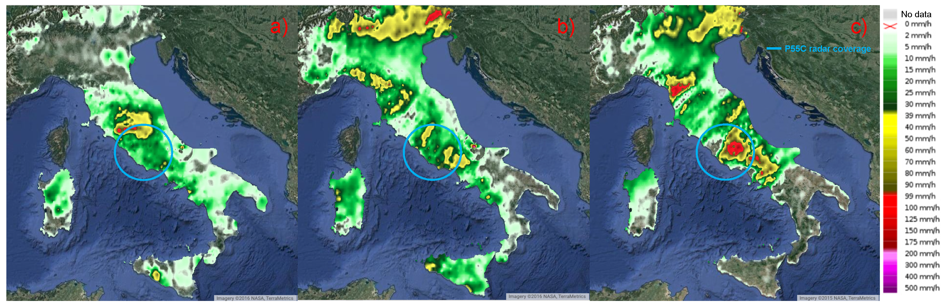
The three cases studied occurred in Italy on 12 and 15 October 2012 and 14 October 2015 in the area surrounding Rome were analyzed. Some of these cases, and in particular those that occurred in 2012, were used in [9] to investigate the relation between the occurrences of lightning and the radar retrievals of integrated water content. For the sake of clarity, 
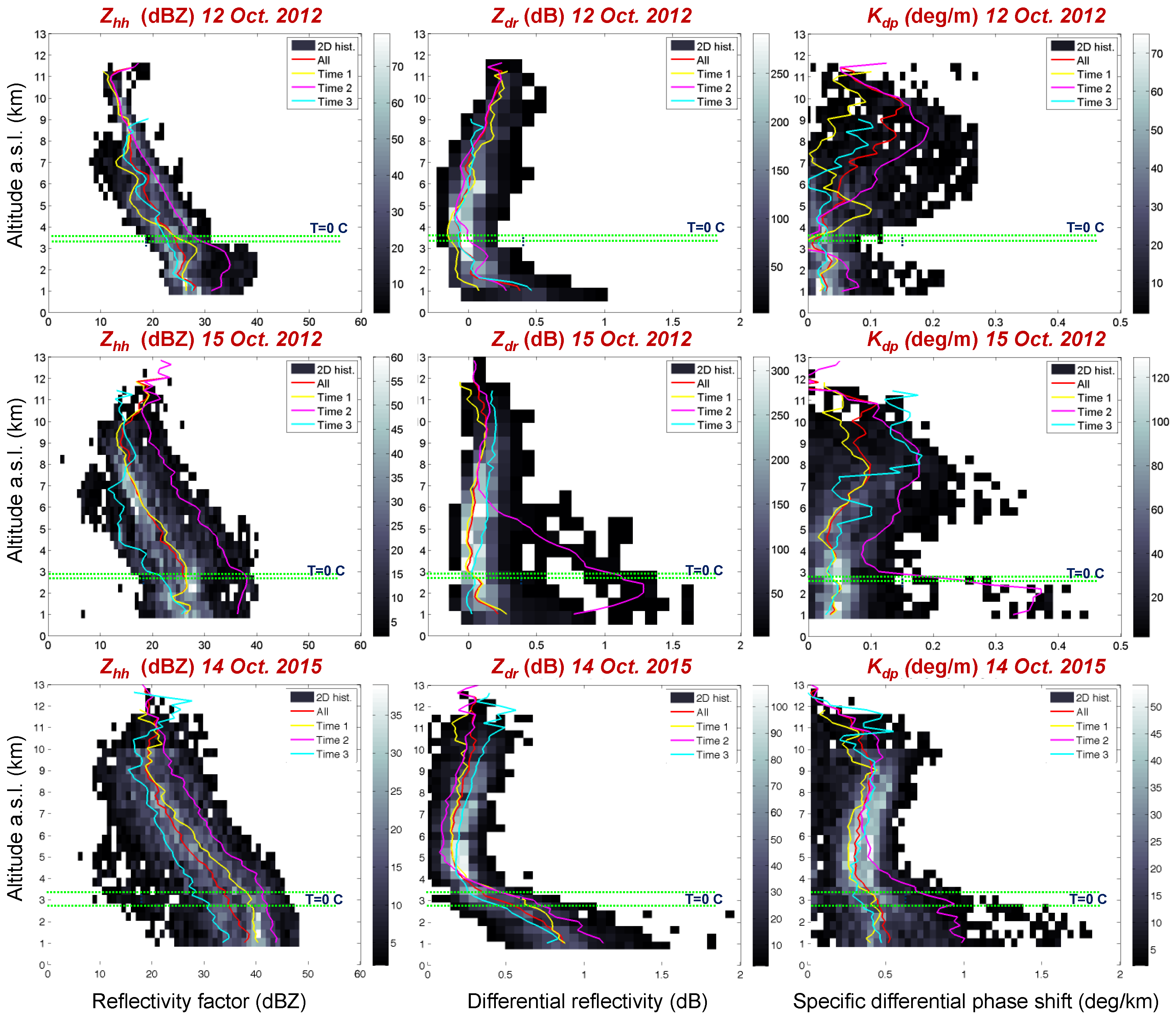
Figure 1 shows the interpolation of the rain accumulations registered on the Italian peninsula over a time interval of 24 h by local rain gauges for those three case studies. The P55C coverage is also shown to better highlight the studied area. In addition,
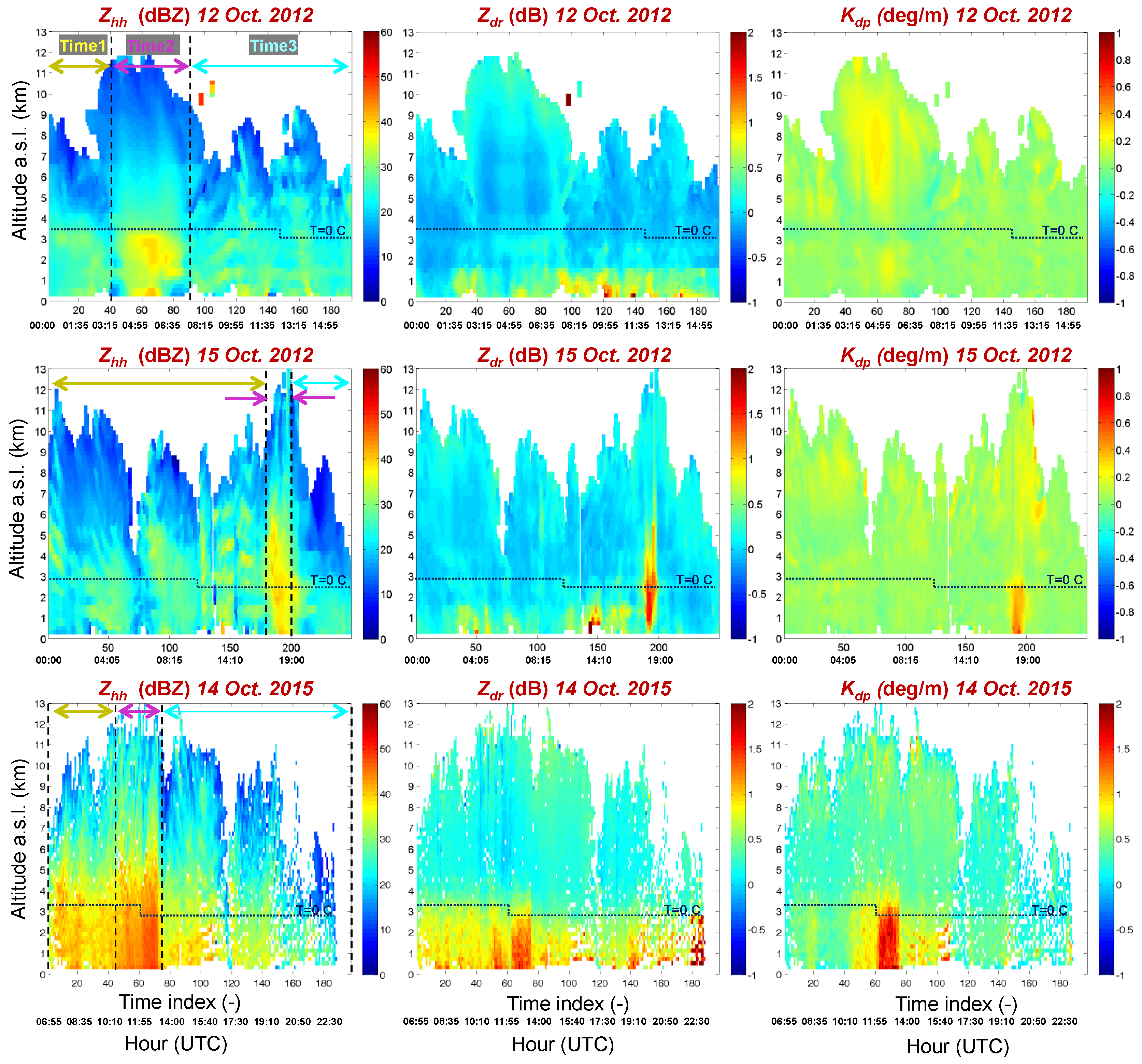
 Figure 2 and Figure 3 give a compact view of the rainy events seen by the P55C radar in terms of time series of quasi-vertical profiles of Zhh, Zdr, and Kdp and their temporal average, calculated using Equation (5), respectively. It follows a synthetic summary of the three events considered.
12 October 2012. This event, associated with a secondary trough over the central Mediterranean Sea, carried heavy precipitation mainly over the Lazio and Umbria regions on 11–12 October 2012. The storm started over the Tyrrhenian Sea, where several mesoscale convective systems developed during the night of 11 October. Convective systems reached central Italy in the early morning of 12 October, with heavy precipitation over the northern part of the Lazio and Umbria regions. The rain was not persistent, but the maximum cumulative rainfall registered exceeded 150 mm in 6 h (Figure 1a). The P55C radar was able to observe only part of the convective systems, mainly beyond 80 km from the radar site. In the last part of the event, the system moved to the south and farther away from the radar (100 km). The main activity developed between 03:15 UTC and 08:35 UTC, as shown in Figure 2, top left, where the time series of the quasi-vertical profile of Zhh is shown. In terms of temporal averages of quasi-vertical profiles, Figure 3, top panels, shows the mixed nature of this event, with a stratiform rain regime at the beginning (labeled Time 1 in Figure 2 and Figure 3) with the typical pronounced peak of Zhh just below the freezing level, lower values of Zdr near zero close to the ground, and accompanied by low values of Kdp. Within the main phase (Time 2), the quasi-vertical profile of Zhh moved to higher values with nearly constant behavior below the freezing level.
15 October 2012. This event took place on 14 and 15 October 2012 across a vast area in the western Mediterranean. The regional weather service issued a severe weather warning for central Italy and particularly for the city of Rome. The precipitation event was associated with a trough that deepened significantly over the northern Tyrrhenian Sea, pushed a frontal system eastward, and advected moist air from the Tyrrhenian Sea inland to fuel deep convection on the coast west of Rome. The synoptic scale system moved rapidly to the east and triggered a line of convection that crossed the western half of central Italy from north to south in a few hours. Most of the precipitation produced by this system occurred in the late afternoon of 15 October across the western part of central Italy and on the western slopes of the Apennines chain (Figure 1b). The main core of the event developed around 17:30 UTC, when a line of convective cells evolved quickly, then started to weaken after 19:00 UTC (Figure 2, middle left panel). The total rainfall amount recorded in Rome was less than had been predicted. The highest daily amount recorded within the historic area of Rome was modest and equal to 35 mm by operational rain gauge. This event is quite characteristic because it clearly shows a Zdr tower during the core phase (Figure 3, middle center panel, “Time 2” curve). The time average profiles in Figure 3, middle panels, show the convective origin of this event and confirm the values of Zdr larger than zero well above the freezing level.
14 October 2015. During October 14 and 15, 2015, strong thunderstorms accompanied by strong winds and heavy rain swept up several regions along central and southern Italy as well as the western and northwestern Balkans, causing floods and landslides across the affected areas. In central Italy, in the Lazio and Abruzzo regions, within the P55C radar coverage, authorities reported landslides and casualties caused by river overflow. In those regions, the extreme weather left three people dead and residents were evacuated for safety on 14 October 2015. A woman died in the town of Paliano near Frosinone after the car she was in fell into a crater that opened up due to flooding after torrential rainfall in the area. Closer to Rome, the Aniene River overflowed its banks at Tivoli, flooding homes and basements and driving some residents onto their roofs for safety. Official sources said 100 people were evacuated from the town of Canistro in the province of L’Aquila in the hills surrounding Rome after the Rio Spalto overflowed. The city of Rome was spared most of the bad weather, while surrounding towns and cities were mostly impacted. The single railway line connecting Rome and Cassino was taken out of action by a landslide. Local rain gauges registered peaks larger than 170 mm within 24 h (Figure 1c). This event was characterized by a severe convection phase with Zhh maximum values up to 60 dBZ and vertical maximum extension up to 10–12 km, Zdr values reaching 2 dB close to the surface and, at some times, extending with positive values over the zero temperature level and Kdp values around 2 deg/km (Figure 2 and Figure 3, bottom panels).
It is worth noting, as with all the case studies discussed here, that the shapes of the average vertical profiles were pretty similar to those found in [24] for convective and stratiform rain regimes. A particularly distinctive signature of such average profiles is noted for Zdr and Kdp, which start sharply increasing just above the freezing level and below it, with different strengths probably depending on the degree of convection of the specific event. This characteristic shape can modify in the presence of Zdr towers or ice crystal aggregation processes.

3.2. Radar System Specifications

The Polar 55C (P55C) is a research-grade C-band (working at 5.6-GHz carrier frequency, 5.35 cm wavelength) Doppler dual polarized coherent weather radar managed by the Italian CNR-ISAC. Differently from most commercial weather radar systems working with the transmission of simultaneous polarization, the P55C system was designed to operate with a polarization agility and single receiver scheme. This means that the total power is alternately transported by the horizontal and vertical polarized signals thanks to a fast switch that allows the transmitted polarization state to be changed on a pulse-pulse-basis. The reception of the horizontal and vertical polarized components alternate as well. This has a direct implication for the dual polarization variables (especially Zdr), whose quality is expected to be higher than in the systems making use of simultaneous transmissions as the power transmitted is fully transferred to the two orthogonal polarization states.
Due to bus data transfer limitations in the signal processor compared with the number of bits used for encoding the radar variables and their required precision, the output quantities of P55C are only Zhh, Zdr, differential phase shift (φdp), and the Doppler velocity (V).
The P55C is located 15 km southeast of Rome (lat.: 41.8425 N deg, long.:12.6464 E deg, 102 m above sea level) on the roof of the ISAC-CNR. The receiver/transmitter apparatus is a fully coherent one. The transmitter is based on a klystron amplifier which allows for very high pulse-to-pulse and phase stability and uses a nominal peak power of 250 kW. For the data collected, considering PRF and antenna rotation speed, the radar measurements were obtained by averaging about 100 pulses transmitted with a 1250-Hz pulse repetition frequency in range bins spaced 75 m apart. The maximum unambiguous radar range was 120 km. The antenna geometry is a single offset type. This allows obtaining an increased radiation efficiency, avoiding beam blocking by stalls, which could both increase the cross-polarization level and cause differences in radiation patterns in the horizontal and vertical polarizations.
Nominal half-power beam widths are 0.92 and 1.02 deg in azimuth and elevation, respectively. The antenna is not protected by a radome and a direct implication is that we do not have limitations due to radome-induced effects (e.g., wet radome attenuation, azimuthal inhomogeneity, cross-polarization couplings). On the other hand, strong winds can make the antenna operations difficult and the pointing might not be accurate in windy situations. However, for the present study the core of the events analyzed was far enough from the radar most of the time, and the wind on the radar site did not cause particular issues. It is worth highlighting that P55C is a weather radar for research, which gives it a larger flexibility with respect to operating systems. For example, during the rain events, the schedules and the scanning strategies can be changed to optimize the observation capabilities.

3.3. Available Measurements and Settings for the Analyzed Case of Study

For the analyzed events the radar antenna elevation sweeps with respect to the horizontal were set to 0.6, 1.59, 2.61, 4.40, 6.20, 8.28, and 11.00 deg. They built up a radar polar volume that was delivered every 5 min. For the case studies, observations covered time windows from 06:55 UTC to 23:55 UTC, from 00:00 UTC to 16:00 UTC, and from 00:00 to 23:55 for a total of 193, 249, and 197 polar volumes for each acquired radar variable on 12 October 2012, 15 October 2012, and 14 October 2015, respectively.
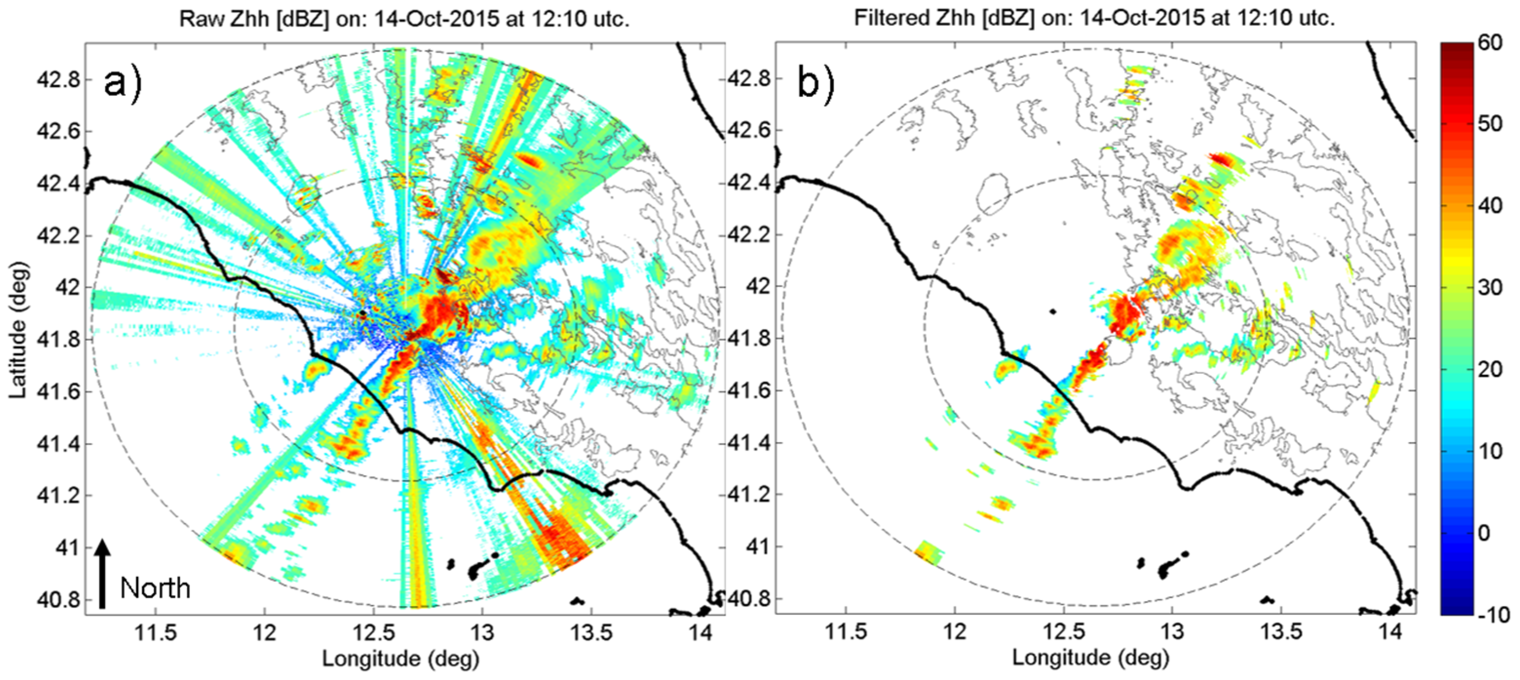
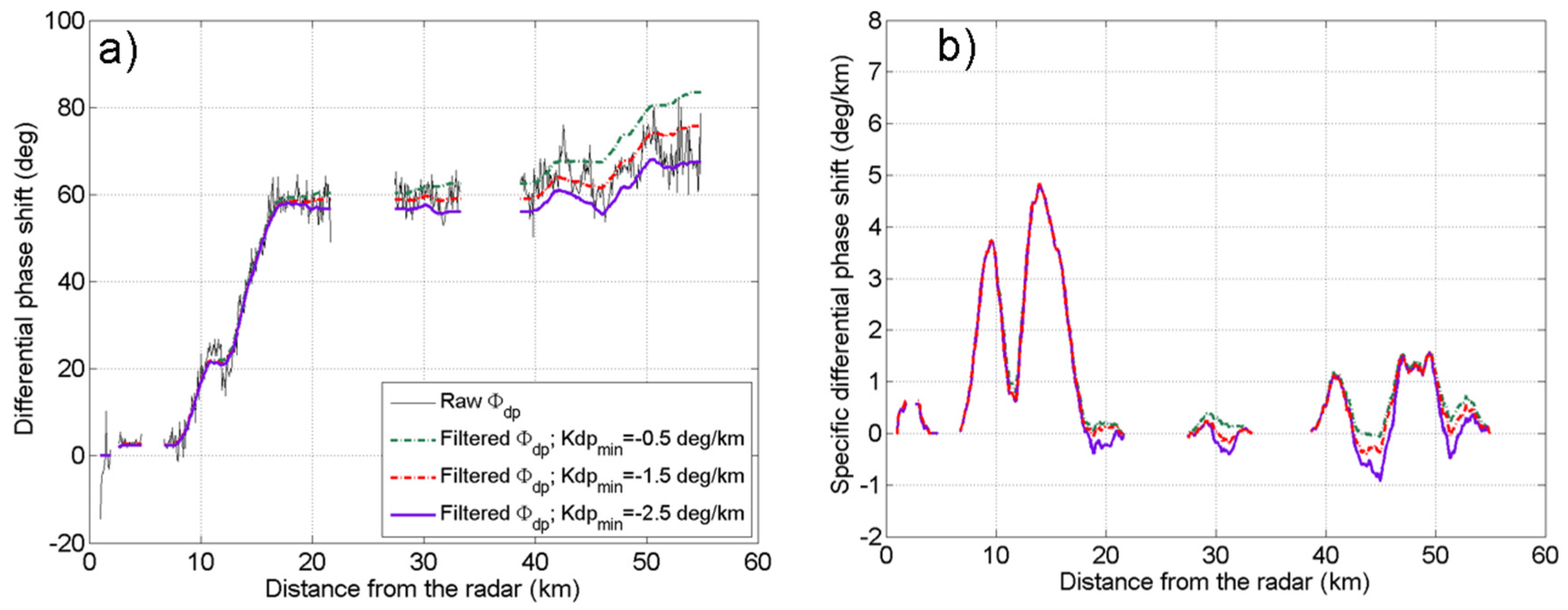
Some range height indicators (RHI) and vertical pointing scans were also scheduled during 14 October 2015 to allow insights into vertical structures of precipitating systems and to deal with Zdr calibration issues. Three sequences of RHI were performed. Sequence 1 includes RHIs at 13:11, 13:17, and 13:21 UTC for the 66 deg azimuth; Sequence 2 includes RHIs at 13:30 and 13:31 UTC for the 190 deg azimuth, and sequence 3 includes RHIs at 13:34 and 13:36 UTC for the 90 deg azimuth. Useful vertical scans were available from 08:10 to 08:14 UTC, for a total of 2160 vertical profiles.
Reference rain gauges were used for comparison with radar QPE. We used rain gauges delivered from the DEWETRA platform, a real-time integrated system for hydro-meteorological and wildfire risk forecasting, monitoring, and prevention. DEWETRA is developed by the CIMA research foundation and is fully operational at the Italian National Department for Civil Protection [34].
Among other information, DEWETRA collects and stores, on an hourly basis, most of the rain gauges of the local weather services in Italy. A total of 293 rain gauges fall in the P55C radar domain after discarding those stations that show anomalous isolated spikes in terms of hourly rain accumulation greater than 300 mm.

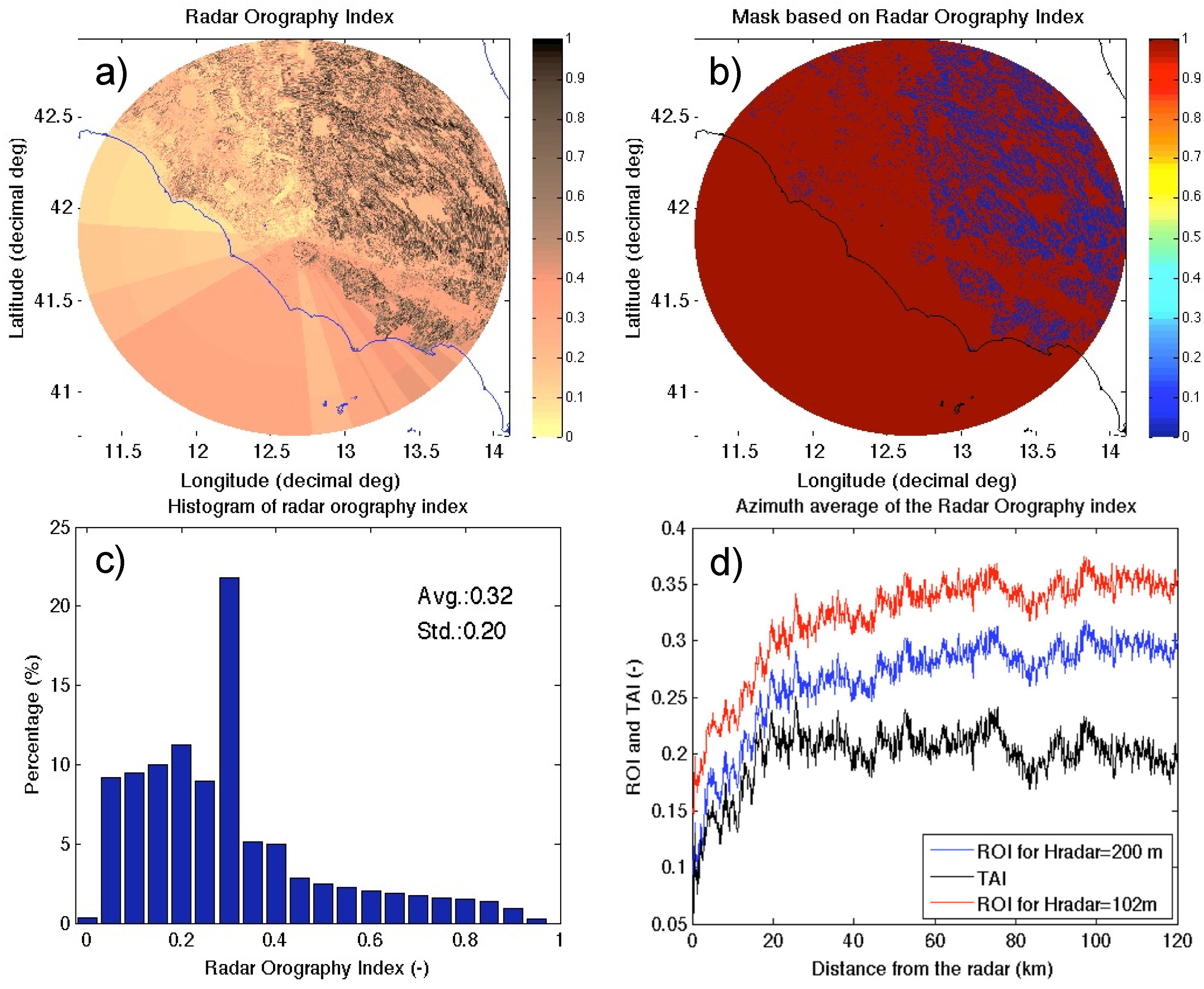
3.4. Definition of Complex Orography

The area covered by the P55C, as shown in Figure 1, is situated in a diversified environment in terms of variation of terrain altitude. This is a situation often referred to as complex orography. As far as the authors were able to ascertain, there is not a unique and objective definition of complex orography, especially in weather radar studies. Indeed, this is a concept that is often more driven by common sense than by rigorous definition. In this section, we want to make a contribution regarding the definition of a complex orography environment for weather radar studies. The first goal in the analysis of the complex orography environment is to define a new parameter that takes into account both the features of the terrain altitudes and the radar geometry of view. For this reason, we define a radar orography index (ROI). ROI can be useful, for example, for comparing different works dealing with QPE in complex orography, fostering a quantitative categorization of previous and future studies by the degree of complex orography seen by the radar.
The complexity of the orography can be described by the gradient of the terrain altitude (GTA). However, GTA alone does not take into account the radar perspective. For example, a radar system positioned on the top of a mountain or in a valley nearby will likely have different QPE performance although the surrounding environment does not change (i.e., GTA is the same within the radar coverage domain). For this reason, we consider an additional term, which is the gradient of the radar beam altitude (GBA). In this way we can define the gradient of the radar orography GRO as follows:
G R O ( p ) = [ ( G T A ( p ) ) 2 + ( G B A ( p ) ) 2 ]    0.5 = [ ( Δ r h T A ( p ) δ r ) 2 + ( Δ r h B A ( p ) δ r ) 2 ] 0.5
where at each position p the operator ∆rhX is the difference of the altitudes hX along with the radial direction, and where δr is the radar radial resolution. The symbol “X” stands for “TA” or “BA”, indicating the terrain altitudes and sampled radar beams altitudes with respect to sea level. Note that in flat terrain and when considering PPI (plan position indicator) acquisitions, GBA coincides with the local tangent of the antenna elevation angle. In that special case, sampling at higher elevations produces higher GRO. In general, the term GBA increases GRO as a function of the radar position and the sampling strategy adopted, (e.g., PPI or LBM: lowest elevation beam or VMI: vertical maximum intensity, etc.). A practical example that will be discussed later on will help to clarify this aspect. So far, Equation (8) is not general enough for practical use in different contexts. In order to constrain the dynamic of GRO to the interval [0, 1] we use an exponential compression formula that allows defining the ROI as follows:
R O I = 1 exp ( b G R O )
In Equation (9) the coefficient b is chosen so that when GRO reaches its maximum value, ROI = 1 (b = 1/max(GRO)). However, to avoid having the few peaks of GRO corrupt the ROI, we considered the 90th percentile (prc90) of GRO instead of its maximum (b = 1/prc90(GRO)).
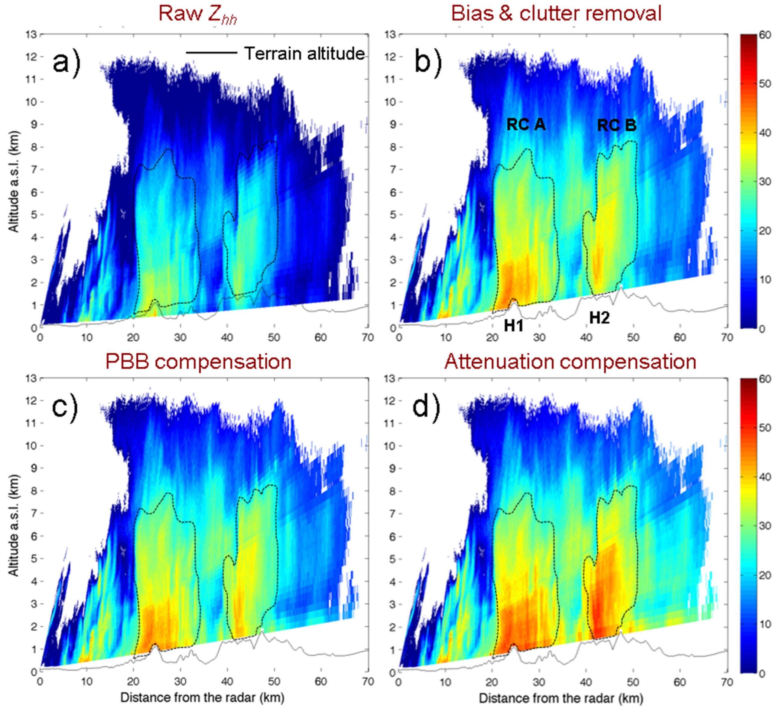
For the P55C we calculated ROI assuming an ideal LBM product. The outcome of this calculation is shown in Figure 4a. Figure 4b shows a mask buildup by applying a threshold to ROI; that is, assigning 0 to positions having ROI >0.6 and 1 otherwise. This mask can be of some practical use for selecting portions of the radar coverage having a reduced impact of complex orography. Figure 4c shows the distribution of the ROI values, whereas in Figure 4d we have drawn average ROIs in two cases: an ideal case where the P55C is positioned at a virtual altitude of 200 m in its actual longitude and latitude position and the actual case, where it is at the altitude of 102 m. In addition, we added the curve of the terrain altitude index (TAI), which is calculated using Equation (9) when GTA is considered instead of GRO. These three curves highlight the sensitivity of ROI to the altitude of the radar position with respect to the surrounding terrain orography. In addition, the separation between ROI curves and TAI highlights the contribution of GRO with respect to GTA. In the result sections below, the mask in Figure 4b is used to evaluate the performance of QPEs in different portions of the P55C coverage domain.

4. Results

Results are shown in the form of comparisons of radar rain estimates vs. rain gauge accumulations for the three events studied here. The rain intensities derived from P55C radar, available on average every 5 min, are accumulated on hourly time scales and then are further summed on larger time window to produce multi-hour accumulations. To make the radar-derived rain accumulations temporarily consistent, we considered only those hours where all the 5-min volume acquisitions were available. In doing so, all radar hourly accumulations were made up by considering 12 radar volumes.
Equations (1)–(4) were used to perform estimations of rain rate intensities, Rq, using single and dual polarization measurements sampled at the lowest elevation beam (LBM), i.e., at positions p = pLBM. In addition, Equation (7) was coupled with the four rain estimations in Equations (1)–(4) to carry out the adjustments related to the vertical variability of the rain precipitation and produce estimations at the positions of the ground levels, p = pGRD. Equation (7) was used in combination with Equation (6) where hm = 0 and the coefficients p1 and p2 are dynamically calculated at each time step. In this respect, 
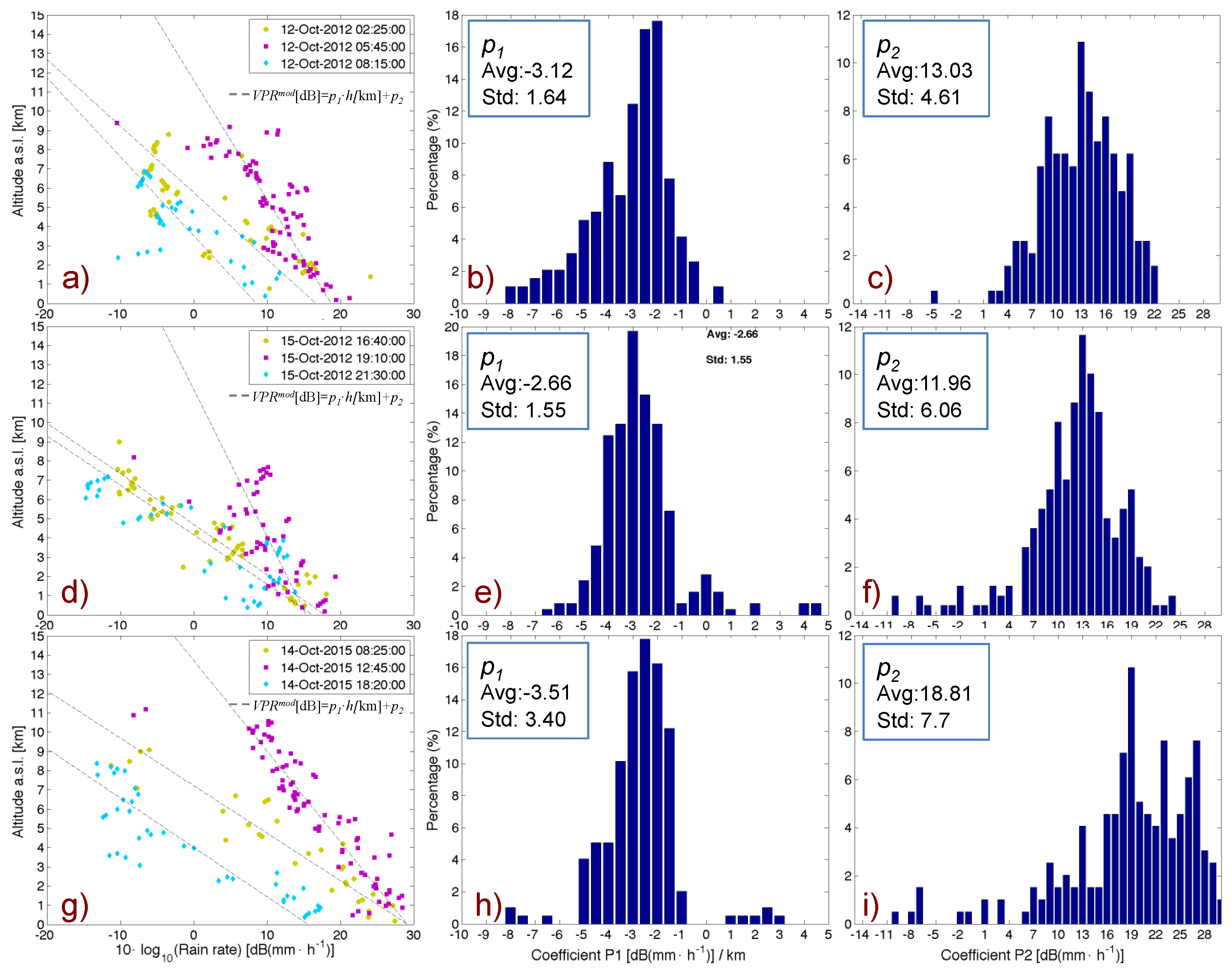
Figure 5a,d,g, show an example of quasi-vertical profiles of rain estimates and its regression model VPRmod as formulated in Equations (5) and (6), respectively. Figure 5b,c,e,f,h,i, show the statistical distribution of the coefficients p1 and p2, respectively, for the entire event. It is worth noting that despite the variability of the events, the coefficients p1 and p2 are quite stable in terms of average and standard deviation. As a first approximation, the average values of p1 and p2 can be used as constant parameters in Equation (6) to adjust the rain estimates aloft and produce estimates closer to those registered at the surface.
To pair the radar estimates and gauge observations, we considered the median of the values of radar hourly accumulations within a circular domain around each rain gauge position. Such choice should smooth the effects due to the time delay needed for the water to fall to the ground as well as the area to point mismatches between the two measurements. The ray of the circular domain is set to 5 km, consistent with typical values of drop fall velocity and horizontal movements of storms. Note that the P55C did not cover the 24 h with a constant time sampling. We limited the rain accumulations only to the hours where the radar variables were available every 5 min, as previously specified.
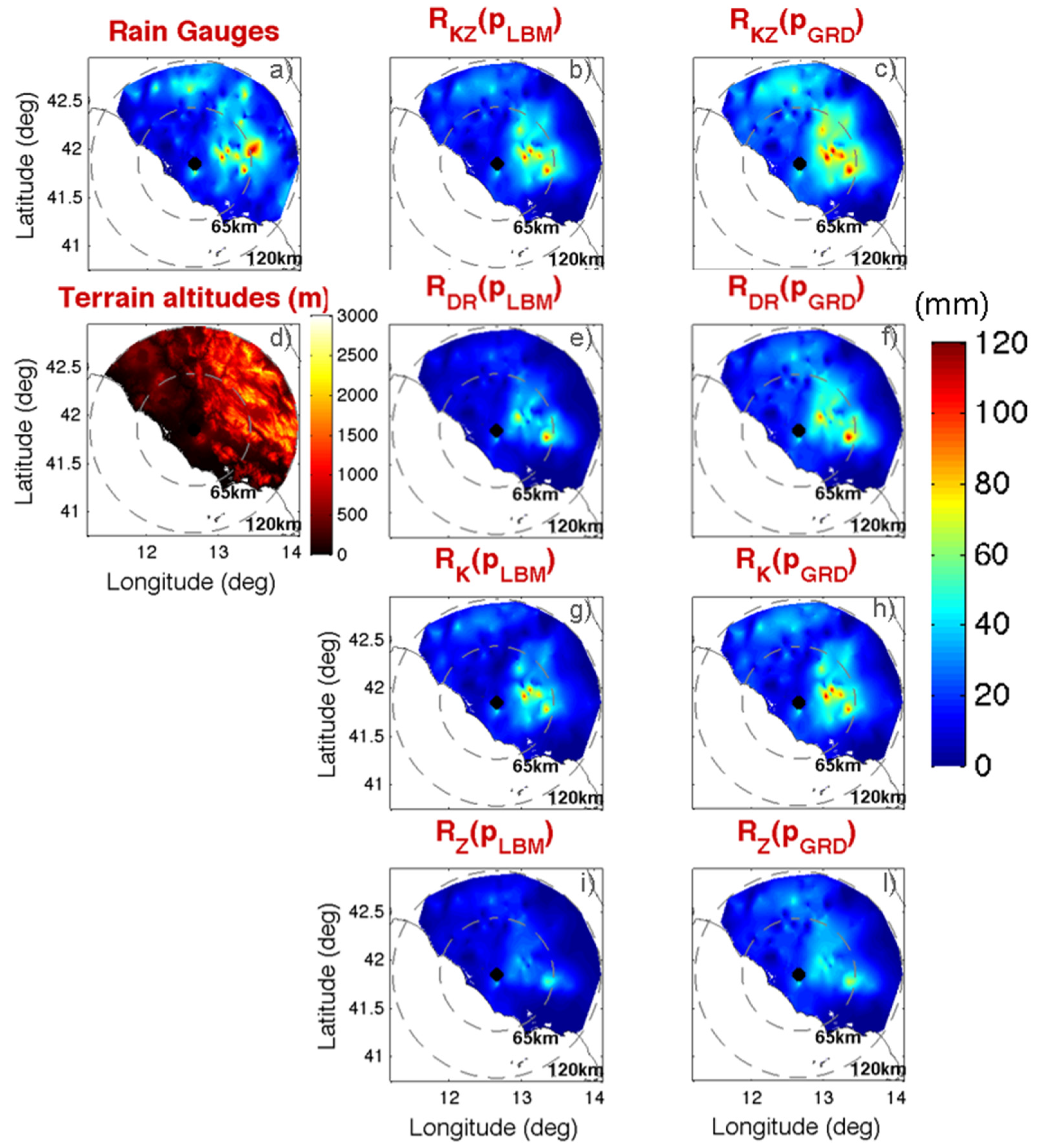
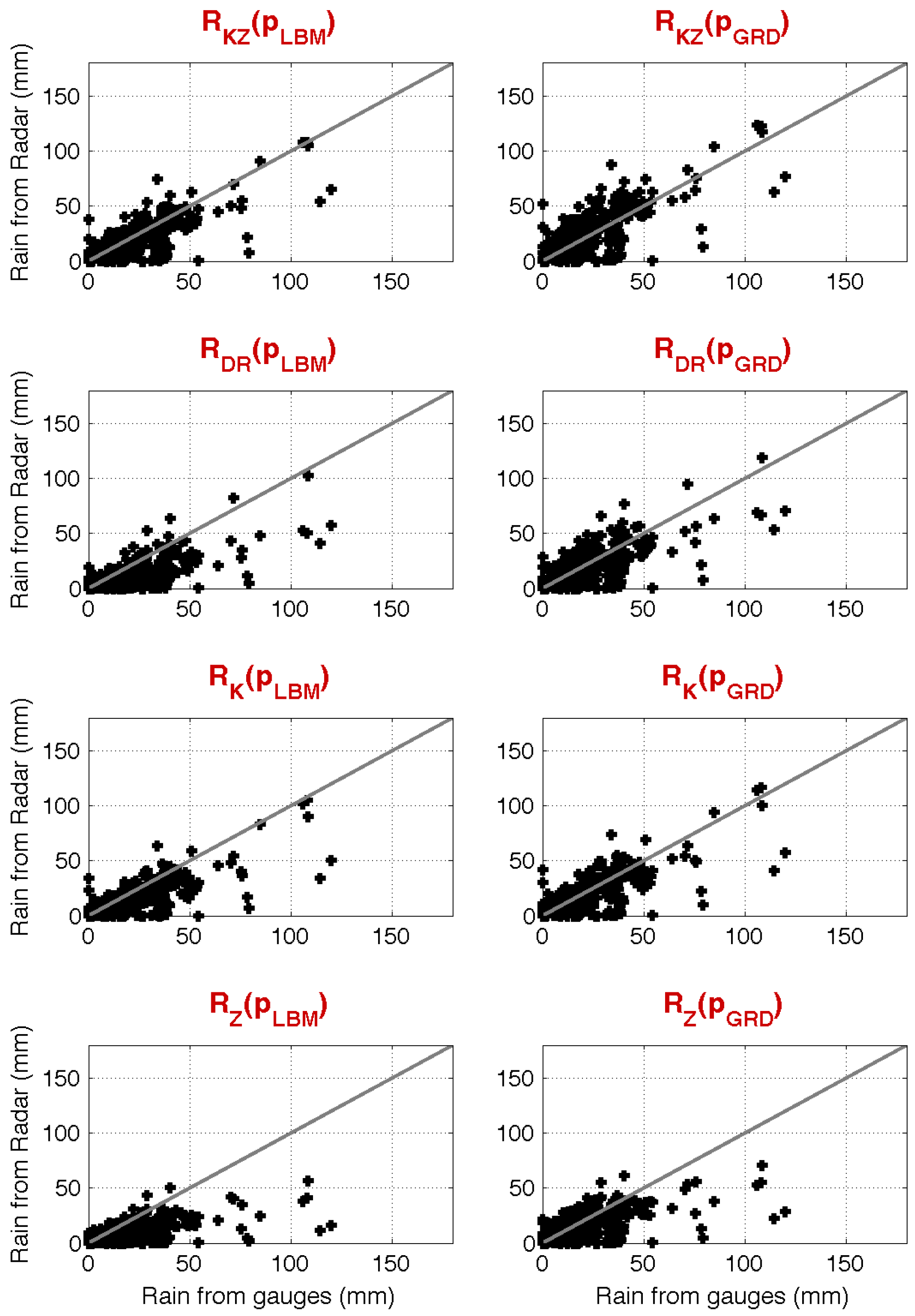
For an immediate comparison of the performances of the various rain estimators considered for all the events simultaneously, Figure 6 shows the total rain accumulation of the events on 12, 14 October 2012 and 15 October 2015. Actually, to make the comparison more homogeneous and highlight the differences among the various QPE algorithms, we considered the values of the total rain accumulations from the radar at the positions of the rain gauges and then we interpolated them on the radar domain. The same was done for the total accumulations from rain gauges. As can been seen from the rain gauge accumulations (Figure 6a) the heaviest precipitation was accumulated mainly inland in the eastern area with respect to the radar position, where terrain altitude variations are more pronounced (Figure 6d). Over all, from this figure a qualitative ranking of the rain estimation algorithm can be done. Looking at the middle column of panels, where the total accumulations of Rq(pLBM) are shown, we can see RZ(pLBM) behaves most poorly, with large underestimations (Figure 6i). A large improvement occurs when using RK(pLBM), which seems to correctly represent the area of heavy precipitation (Figure 6g). When introducing Zdr; i.e., when using RDR(pLBM), (Figure 6e), we have a small improvement with respect to RZ(pLBM) but we still register an appreciable underestimation compared to RK(pLBM). Finally, when combining all RK and RDR into a single rain estimator, RKZ(pLBM), (Figure 6b), we have something that is more consistent with the rain gauges with respect to using RK(pLBM) alone. On the other hand, when applying the quasi-vertical profile adjustment (panels in the right columns of Figure 6) we have an increase of rain precipitation values for all the implemented estimates and a more qualitative agreement with rain gauges, especially in the tendency to represent the maxima of accumulated precipitation (compare, for example, Figure 6g,h with the reference Figure 6a). A confirmation of this is given in the example shown in 
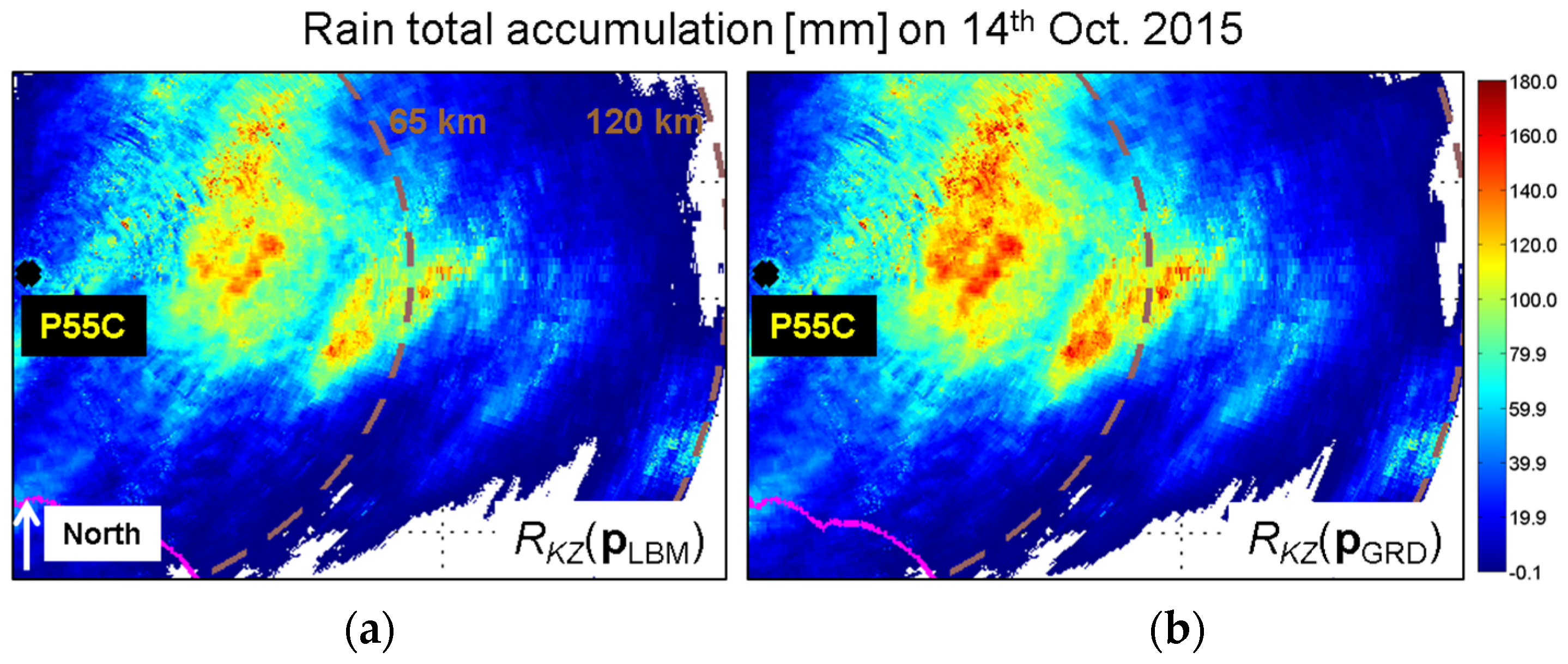
Figure 7, where a zoomed version of RKZ(pLBM) and RKZ(pGRD) is displayed for the case of 14 October 2015. This figure can be particularly informative in the light of combined radar and rain gauge products. Indeed, in these merging approaches and in particular for those that make use of the Kriging methodology, the spatial structure of the rain field from radar, usually described in terms of spatial covariance or variogram, is used to train the interpolation algorithms [35]. As is evident in Figure 7, the spatial structure of rain precipitation fields changes depending on the effect of the spatial adjustment performed (quasi-vertical profile adjustment in our case), and this effect can cause variations in the final results of the combined radar vs. rain gauge products.
To complete the examination of the results, Figure 8 shows rain estimator comparisons in terms of total accumulations of radar vs. gauge scatter plots for all the events. Although we note the presence of a significant number of mis-detections (i.e., rain gauge registers rain whereas the radar does not register it), it seems that the use of Kdp is a key factor when estimating rain in complex orography environments, whereas the use of quasi-vertical profile adjustment is able to partially compensate for the overall bias, although the differences in this case can be subtle. For example, note the distribution of sample pairs around the reference 1:1 line and the error scores discussed below. On the other hand, the estimated precision (the variability of the estimates around the 1:1 line) seems to not get a strong benefit from the application of quasi-vertical profile adjustments.
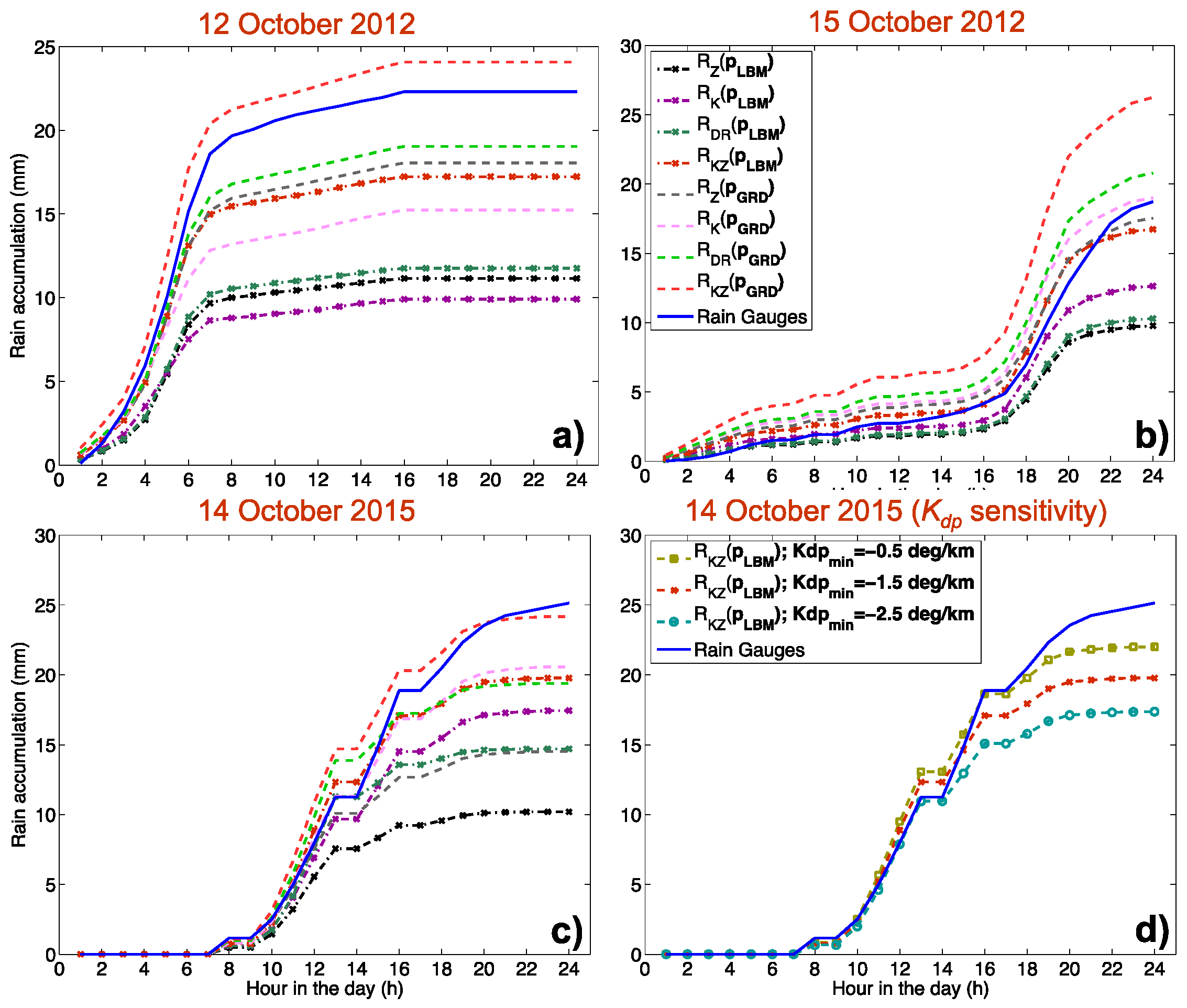
In terms of spatial averages of rain accumulations over time, a clear performance evaluation is shown in Figure 9 for each case study. Figure 9a,c confirms the best performance of RKZ(pGRD) (red dashed line, which shows the results closest to the blue curve of the rain gauge total accumulation). On the contrary, for the case on 15 October 2012 (Figure 9b) we have a different outcome, with quite a large overestimation of RDR(pGRD) and RKZ(pGRD) and the best performance obtained when considering RZ(pGRD) or RK(pGRD). Finally, it is worth noting that the performance of the Kdp-based rain estimator depends to some extent on how it is retrieved. In particular, Figure 9d, shows the performance of RKZ(pLBM) as a function of four thresholds used (Kdp_min) for the retrieval of Kdp as specified in the figure legend for the case study on 14 October 2015. See Appendix A and Figure A3 for more details on the filtering of the differential phase shift (φdp) and Kdp estimation. For the analyzed cases we used Kdp_min = −1.5 deg/km, which seems to be a reasonable choice in terms of φdp filtering.
Looking at more quantitative results, Table 2, Table 3 and Table 4 list the root mean square error, the normalized standard error, the normalized bias, and the correlation coefficient, labeled as RMSE, NSE, NB, and CC, respectively, and defined in Appendix B, for the various rain estimators implemented for the three case studies. In these tables we also included the error scores obtained when applying a gauge-bias adjustment factor (AF) to Rq(pLBM) since many operational QPE algorithms use a gauge-bias correction procedure to fold all of the error sources that compromise the QPEs. Basically, AF is an average ratio of rain gauge accumulations with respect to those from radar estimates as a function of the distance from the radar. We described AF using an exponential law and derived its regression parameters for each of the Rq(pLBM) algorithms in Equations (1)–(4) by considering the three case studies together. In addition, the right column in each table lists the average relative improvement between Rq(pLBM) and Rq(pGRD) when they are evaluated for two distinct parts of the radar domain: the domain where ROI ≤ 0.6 (lower degree of complex orography) and ROI > 0.6 (higher degree of complex orography).
From the tables, we note that there is a maximum improvement of approximately 20% in terms of root mean square error (RMSE) when applying a quasi-vertical profile adjustment on an RZ estimator (i.e., when moving from RZ(pLBM) to RZ(pGRD)), although the increment was as low as 4% in the case on 15 October 2012 (Table 3). The biggest improvement, as noted previously, is made when using RK. In this case, the improvement from RZ(pGRD) to RK(pGRD) is between 18% and 30%, with the exception of 15 October 2012, where the improvement reaches only 7%. The combined rain estimator, RKZ, gives a further small improvement between 6% and 10% with respect to RK(pGRD) and between 30% and 38% compared to RZ(pGRD). Even in this case, the only exception is given by the performance obtained on 15 October 2012 that register a deterioration of RKZ(pGRD) with respect to the other estimators when quasi-vertical profiles are used. Actually, the strongest improvement brought by the use of quasi-vertical profile adjustment seems to be in terms of normalized bias, with results significantly reduced by a factor larger than 25% when moving from RZ(pLBM) to RZ(pGRD) and from RKZ(pLBM) to RKZ(pGRD) on 12 and 15 October 2012.
In terms of the adjustment factor (AF), its impact is to increase the correlation coefficient a little bit and in some cases to reduce the bias, but at the same time to produce larger RMSEs. On the other hand, when partitioning the radar scene in the regions most affected by the complex orography (ROI > 0.6) by those with lower complexity (ROI ≤ 0.6), we find that the impact of quasi-vertical profile adjustment is, in most of cases, larger (i.e., more negative) than that in the areas with lower complex orography, as expected. Note that ROI is correlated with QPE; that is, larger ROI corresponds, in most of cases, to larger RMSE. However, to maintain a reasonable size for Table 2, Table 3 and Table 4 we did not list all the error scores as a function of ROI. To have an idea of the correlation of ROI with the RMSE when all the QPE algorithms with no correction are considered, we list the average, standard deviation, and maximum RMSE for ROI ≤ 0.6 and ROI > 0.6, (18.37, 3.80, 27.41) and (25.92, 14.41, 53.67), respectively.

5. Discussion

From the results just presented one notable aspect is an ambiguity in the interpretation of the results regarding the identification of the best robust rain estimator among the various case studies. In most of the analyzed cases in this study, the combined RKZ with the use of quasi-vertical profile adjustment seems to perform better than the others, although an exception exists. Recent literature on QPE studies seems to be more oriented toward a combination of various QPE algorithms whose choice can guided by information related to the type of precipitation [22,26,27]. In this respect, the concept of adjusting rain estimates using quasi-vertical profiles of rain, VPR, as introduced in this work can add to the existing techniques. The advantage of using quasi-VPR is that it allows adjusting rain estimates from its vertical variability in a direct and self-consistent way. However, complications in using quasi-VPR can arise because its variability reflects that of the QPE algorithm used. In other words, the shape of the VPRs depends on the specific QPE algorithm used, and a characterization of the VPR for each QPE algorithm would be needed. For example, we expect that a VPR obtained considering RK will have a lower negative slope than RZ in the ice part given the typical values of Zhh and Kdp in the ice region. Then, an ideal procedure that used VPRs and a combination of several QPE algorithms should address this issue. On top of this, the co-existence of different types of precipitation in different radar domains adds complexity to the procedure because a single VPR is unlikely to represent the entire radar scene. Thus, a more sophisticated VPR retrieval would require the separation of the observed radar scene in areas of different precipitation types. Then, for each of those areas we should identify a characteristic VPR and apply the adjustment separately. This lack of further sophistication is probably responsible for the larger errors found when applying the VPR adjustment for the event on 15 October 2012. In that case, another aspect to highlight is the fact that the QPE algorithms we are using do not take into account peculiar situations such as, for example, Zdr columns. For this reason, in general, caution is needed when dealing with QPE algorithms that are based on Zdr. A last issue that would need to be addressed when dealing with quasi-vertical profiles is that they are “apparent” (i.e., they are the result of the antenna pattern convolution with the actual unknown measured quantity) and obtained using slant observations. This consideration is open to the possibility of further refinement, which should include the identification of the actual VPR using deconvolution techniques [36] and estimation theory e.g., [37].

6. Conclusions

This work analyzed three case studies of heavy rain precipitation in Italy that affected the Roman area and caused damage and three casualties, as reported by local news. The C-band dual polarization radar Polar 55 C (P55C), managed by the Institute of Atmospheric Sciences and Climate (ISAC) at the National Research Council of Italy (CNR), tracked the events. The work focused on two aspects scarcely considered by past studies on radar rain estimation: (i) a proposal to objectively define the complexity of an orography scenario with respect to the radar standpoint; and (ii) an evaluation of the benefit brought by the vertical profile extrapolation when using dual polarization QPE algorithms. P55C coverage is well suited to pursue these goals because it includes quite flat regions as well as a part of the Apennine chain with terrain peak altitudes higher than 1500 m and a difference in the P55C radar lowest available bin altitudes and gauge stations of 1240 m on average, with maximum values up to 6 km.
The comparison of radar QPE with rain gauge accumulations indicates that the combined algorithm, which merges together, through a weight factor, the differential phase shift Kdp, the single polarization reflectivity factor Zhh, and the differential reflectivity Zdr, once accurately post-processed, performs better in most of the cases tested than those that make use of Zhh alone, Kdp alone, and Zhh and Zdr. An improvement larger than 25% is found in terms of normalized bias when applying VPR extrapolations to Zhh-based QPE and to the combined QPE algorithm. Many limited improvements are registered in terms of root mean square errors because the error standard deviation probably accounts for most of the discrepancies registered between radar QPE and reference rain gauge.
An additional aspect that emerges from the analysis is that the quality of the Kdp estimates, through its filtering, has an impact on the performance of the QPE algorithms, although this impact is less significant when the combined algorithm is considered. In addition, in one case analyzed, where we observed Zdr columns we found that the VPR adjustment produced quite large overestimations, leading us to conclude that methods based on Zdr can worsen the final results if we do not apply any special care in the preprocessing step as well as in the QPE algorithms.
Although further and more robust analysis in terms of statistical significance will be needed to corroborate our findings and validate our methodology, the results of this work point to a possible operational way to improve the radar QPE algorithms based on dual polarization variables in complex terrain. Future work could be focused on the systematic collection of a considerable number of case studies with different precipitation types from other radar systems in Italy to validate the VPR approach.

Acknowledgments

The authors want to thank the Italian Department of Civil Protection of Italy for supporting weather radar studies in Italy. A special thanks goes to Jean Charney for the English editing of the work. The publications costs have been supported thanks to a funding scheme of the University of L’Aquila within the national program SIR (Scientific Independence of young Researchers) 2015.

Author Contributions

Mario Montopoli conceived the manuscript and designed the experiments; Nicoletta Roberto contributed to the selection and critical review of the case studies analyzed. Elisa Adirosi provided the QPE estimation coefficients based on particle size distribution measurements. Luca Baldini gave useful suggestions and material for the processing of the radar variables. Eugenio Gorgucci gave important guidance. Everybody contributed in the discussion of the results.

Conflicts of Interest

The authors declare no conflict of interest.

Appendix A. Processing of the Radar Measurements

The P55C radar variables are accurately processed before using them in the QPE algorithms. The goal of all the processing steps is to maximize the measurement quality: that is, identify and discard noisy acquisitions, minimize the contribution of system miscalibrations, ground clutter returns, radio frequency interferences, beam blocking effects, and path attenuation.

Appendix A.1. Signal-to-Noise Ratio Thresholding

A first step in our radar processing chain is to guarantee that all samples processed in further steps are reasonably above the noise level of the radar receiver. In principle, this can be accomplished by calculating the noise threshold which characterizes the radar receiver and retaining all measurements found above that noise threshold. However, in so doing some technical features of the receiver need to be accurately known or monitored (e.g., the noise figure or the minimum detectable signal of the receiver). In this work we adopted a quick and self-consistent way to filter out the measurements affected by noise without the need to know the nominal characteristics of the radar receiver. In practice, from the radar equation of the received power at distance r, in linear units (P(r) = C·Zhh(rr−2), we can rewrite it in terms of the minimum detectable reflectivity and the minimum detectable power signal abbreviated as MDZ and MDS, respectively. Thus, the radar equation in terms of these minimum quantities is MDZ = C−1·r2 MDS. The filtering of the values affected by noise is accomplished by discarding all values of Zhh lower than MDZ at each range gate r. To do that, only MDS needs to be known (the constant C cancels out with MDS, as will be seen later). This can be done by exploiting the raw data itself. Indeed, we can reasonably expect that in clear air conditions the values of Pr detected at the farthest distances rmax are a good approximation of the minimum level detectable (PminMDS). Such clear air conditions are also met for relatively high elevations at far distances even during a precipitation event. Thus, MDS = C·Zhh(rmaxrmax−2, and when regrouping all terms into MDZ we have MDZ = (r/rmax)2 Zhh(rmax).Then a stable measure of Zhh(rmax) allows estimating MDZ and then filtering out Zhh < MDZ.

Appendix A.2. Clutter Identification and Its Suppression

This task is accomplished using a fuzzy logic scheme that takes as input the textures of Zhh, Zdr, and the unfiltered differential phase shift plus an experimental clutter polar volume obtained by considering time averages of Zhh calculated separately offline. All the above-mentioned information is then weighted using the fuzzy logic scheme as in [20] and well described in [38]. The output quantity of the fuzzy tool we used is a quality index that describes the strength of membership degree of a given grid point within the radar grid to the class of ground clutter echoes with respect to the rest of the possible target typology. Note that since we make use of texture features of input radar variables, their calibration is not strictly required at this step of the processing chain. An interesting behavior that we verified is that the fuzzy approach we used also tends to suppress reasonably well the radio frequency interferences, although this is achieved at the cost of filtering out some of the meteorological features at the border of the rain cells in the clutter class. An example of the clutter filtering outcome is given in Figure A1 where raw Zhh (Figure A1a) is compared with its filtered version (Figure A1b) obtained applying the signal-to-noise ratio thresholding and the fuzzy logic filtering steps. As can be seen from the unfiltered raw data in Figure A1a, the environment is made particularly challenging by the presence of a lot of radio frequency interferences (look at the radial signatures departing from the radar position at the center of the map) that add to the ground clutter more densely present in the eastern part of the map. In Figure A1b, after applying the clutter filtering, all the apparent contaminations due to clutter and radio frequency interferences seem to be reasonably suppressed, although some radar resolution volumes of precipitation might be erroneously labelled as clutter and then put to void values. An additional example of clutter suppression is given in Figure A2b, in terms of an ad hoc RHI acquisition of Zhh, where at the hill peaks, labelled as H1 and H2, the radar signal results were correctly suppressed with respect to raw Zhh in Figure A2a. The same figure also shows the appearance of Zhh when other processing steps are applied, as will be discussed in the following sections of this Appendix.
Figure A1. Example of the outcome of the clutter filtering procedure on 14 October 2015 at 12:10 UTC for a Plan Position Indicator (PPI) at 1.59 deg radar antenna elevation. (a) Raw reflectivity factor, Zhh, (dBZ); (b) filtered version of Zhh after the clutter filtering. Contours of terrain altitudes at 500 and 1500 m asl. (grey contours) and constant range circles at 65 and 120 km from the radar are overlaid.
Atmosphere 08 00034 g010
Figure A2. Example of the outcome of the radar processing chain in terms of specifically arranged Range Height Indicator (RHI), acquired by P55C radar on 14 October 2015, 13:17 UTC at 66 deg azimuth (a); after performing the Zhh (dB) bias compensation and clutter suppression (b); partial beam blocking compensation (c); and single polarization path attenuation compensation (d).
Atmosphere 08 00034 g011

Appendix A.3. Differential Phase Shift Filtering and Kdp Estimation

Several techniques exist for differential phase filtering, which is a key processing step and is the base of Kdp estimation. Past developments on this topic include algorithms based on least-square fitting methods [39], FIR filters [40], wavelet analysis [41], linear programming constraints [42], and, more recently, Kalman filter approaches, which are promising under lower signal-to-noise ratio conditions [43]. All these methods aim at reducing the effects of the statistical errors affecting the measured differential phase (φdp), including those error sources originated by statistical/sampling error, ground clutter, side lobes, second-trip echoes, mixed-phase hydrometeors (large melting aggregates and hailstones), non-uniform beam filling, and to some extent compensating for the effects of the differential backscattering phase (δhv). The final result is a filtered differential propagation phase (φdp) that should be monotonically increasing and not excessively smoothed in order to avoid overly processed Kdp estimates that lose fine-scale precipitation features.
To this goal, in this work we used the phase filtering scheme proposed in [20], which is based on the application of FIR filters applied recursively for the direct estimation of φdp and for its inverse estimation through temporary estimates of Kdp. It has been demonstrated that this approach combines an easy practical implementation with a reasonable degree of estimation accuracy and the representativeness of the final Kdp product in terms of spatial resolution features while using a filter length on the order of 1 km. In addition, this technique allows choosing the level of negative values of the output Kdp (Kdp_min) consistently with the filtered φdp, thus modulating the inclusion of the contributions of δhv, non-uniform beam filling, and other statistical errors, which usually cause negative values of Kdp. Figure A3a, gives an example of raw φdp and some of its filtered versions using various thresholds of Kdp_min, as specified in the panel’s legend. The resulting filtered Kdp are shown in Figure A3b. Note that when selecting Kdp_min = −0.5 deg/km, φdp is forced to be quasi-monotonically increasing for any negative range variation of φdp, leading in that case to an overestimation of raw φdp. However, this does not affect the peaks of estimated Kdp but, instead, its values are closer to zero (Figure A3b). A more conservative choice is given when Kdp_min = −1.5 deg/km, which is the value used in the main text.
Figure A3. Example of differential phase shift (φdp) and estimated Kdp on 14 October 2015 taken at 6.2 deg elevation angle and 107 deg azimuth. (a) Raw φdp (black line) and four φdp filtered versions (colored lines) using several Kdp minimum thresholds (Kdp_min) as specified in the panel’s legend; (b) Estimates of Kdp for the values of Kdp_min specified in the panel’s legend.
Atmosphere 08 00034 g012

Appendix A.4. Partial Beam Blocking Compensation

Partial beam blocking is required for P55C measurements of reflectvity and differential reflectivity since the eastern part of the radar domain is widely intersected by the Apennine chain (peak altitude 2912 m). In those areas, antenna tilts lower than approximately 3 deg can be responsible for the partial occlusion of the radar beam and the consequent lowering of Zhh. In this work, we calculated the partial beam blockage levels (PBBL) representing, at each position and for a specific antenna elevation, the occultation degree varying from 0 (free of blockage) to 1 (totally blocked). This is accomplished by resorting to the simplified obstruction function proposed in [44] and applied to the difference between the terrain altitude and that of the expected radar ray paths. A model for the terrain altitudes is required to run this procedure. In in this work, the terrain altitudes are obtained from the SRTM 90 m digital elevation model database [45]. Then the compensation of Zhh for partial blocking is carried out by multiplying Zhh (in linear units) for a compensation multiplicative factor equal to 1/(1 − PBBL) for PBBL within [0.1, 0.7] (compensating beam obstructions from 10% to 70%). This means applying a multiplicative compensation factor of 1.111 and 3.333, which implies adding factors of 0.4571 dB and 5.2284 dB, respectively.
Figure A2c, shows an example of such PBBL compensation. For example, comparing Figure A2b,c at the bottom right side of rain cells A (contoured with black dotted line and labelled as RC A), the PBBL effect and its compensation is quite evident. Partial blocking from hill H1 propagates also to H2, where a difference of about 5 dBZ is compensated at the bottom of rain cell RC B.

Appendix A.5. Calibration of Zdr

In the present work, the Zdr calibration is verified through vertical pointing of the radar antenna that were available during the analyzed dataset. The measured average value of Zdr (in dB) gives an estimate of its miscalibration being the expected signature of Zdr for rain drops observed vertically equal to 0 dB [46]. For the P55C, for the case studied here we compensated for a miscalibration factor of 2.69 dB with respect to an arbitrary reference factor value, which was verified using vertical observation in rain.

Appendix A.6. Path Attenuation Compensation

The compensation of the rain path attenuation on both Zhh and Zdr is accomplished by exploiting the quasi-linear relation between specific attenuations Ahh, Adr in (dB/km), and Kdp (deg/km), respectively, which is Ahh = αhh·Kdpβhh and Adr = αdr·Kdpβdr. The coefficients αhh and αdr can vary in time and space depending on raindrop size, shape, and temperature. In this work we used the coefficients of αhh, βhh, αdr, and βdr from [47] at C band, which are 0.073, 0.99, 0.013, and 1.23, respectively. Those coefficients are valid in a rain regime only and for this reason we limited their application to in-rain layers only. To do that, we adopted an altitude threshold to identify the bottom of the freezing band. The nearest radiosounding is Pratica di Mare, Italy (Station identifier: 16245 LIRE, lat.: 41.65, long.:12.43, about 28 km far from the radar site), and is used for this purpose. All radar samples below that threshold were compensated for rain path attenuation. Everything above was maintained at the level of the last compensation applied in rain. The value of the zero thermal altitude registered by radiosoundings in Pratica di Mare for the analyzed event on 15 October 2015, was 3218 m and 2895 m asl, at 00 and 12 UTC, respectively.
Figure A2d gives an example of path attenuation compensation, which is particularly evident for rain cell RC B. A maximum compensation of 11 dBZ is registered in this example.

Appendix A.7. Calibration of Zhh

The calibration of Zhh is carried out following the methodology described in [48], where a third-degree polynomial formula relating the ratio Kdp/Zhh as a function of Zdr is proposed to formulate the self-consistency approach proposed in [10]. Thus, we derived the bias that needs to be considered for the calibration of Zhh by minimizing the difference between the measured total differential phase shift for some selected radar samples in light rain and that reconstructed using the third polynomial formula as a function of variable possible values of the bias of Zhh. The total differential phase shift is calculated by adding selected values of Kdp·2 δr along radial paths, where δr is the radar radial resolution in (km). However, we verified that in the above-mentioned procedure the selection of the samples in light rain requires particular attention. To this aim, we excluded the radar grid points that comply with the following rule: KdpKdp_up or hbin > hfl_bt or Zhh > Zhh_up or SdrSdr_dw or Sdr > Sdr_up or r < rdw, where Kdp, hbin, Zhh, Sdr and r is the filtered differential phase shift in (deg/km), the altitude asl. of the radar bin (km), the attenuation corrected radar reflectivity factor (mm6/m3), the standard deviation of the attenuation corrected differential reflectivity, and the distance from the radar (km). The thresholds used are set up as Kdp_up = 0.5; hfl_bt = 3; Zhh_up = 10(60 dBZ/10); Sdr_dw = 0; Sdr_up = 0.05; rdw = 5.

Appendix B. Error Score Definitions

In this appendix the definition of the error score used in this work for the evaluation of the radar and rain gauge comparison is given for the reader’s convenience. These score indexes, although widely used and well-established statistical tools, are often defined in different ways in the various radar quantitative precipitation studies published to date. We define the root mean square error (RMSE), the normalized standard error (NSE), the normalized bias (NB), and the Pearson correlation coefficient (CC) as follows:
R M S E q = < ε q 2 >
N S E q = R M S E q < R g >
N B q = < ε q > < R g >
C C q = < R q μ R q > < R G μ R g > < σ R q 2 σ R g 2 >
where ε is the difference between the rain accumulations from the radar (Rq) and that from the rain gauge (Rg). The subscript q indicates one of the rain estimators used in the main text in Equations (1)–(4). The operator <·> indicates the arithmetic average over the numbers of paired radar and rain gauge rain values. The symbols µx and σx2 stand for average and variance of x, respectively.

References

  1. Hou, A.Y.; Kakar, R.K.; Neeck, S.; Azarbarzin, A.A.; Kummerow, C.D.; Kojima, M.; Oki, R.; Nakamura, K.; Iguchi, T. The Global Precipitation Measurement Mission. Bull. Am. Meteorol. Soc. 2014, 95, 701–722. [Google Scholar] [CrossRef]
  2. Gochis, D.; Schumacher, R.; Friedrich, K.; Doesken, N.; Kelsch, M.; Sun, J.; Ikeda, K.; Lindsey, D.; Wood, A.; Dolan, B.; et al. The Great Colorado Flood of September 2013. Bull. Am. Meteorol. Soc. 2015, 96, 1461–1487. [Google Scholar] [CrossRef]
  3. Sun, J.; Xue, M.; Wilson, J.W.; Zawadzki, I.; Ballard, S.P.; Onvlee-Hooimeyer, J.; Joe, P.; Barker, D.M.; Li, P.W.; Golding, B.; et al. Use of NWP for Nowcasting Convective Precipitation: Recent Progress and Challenges. Bull. Am. Meteorol. Soc. 2014, 95, 409–426. [Google Scholar] [CrossRef]
  4. Sokol, Z. Assimilation of extrapolated radar reflectivity into a NWP model and its impact on a precipitation forecast at high resolution. Atmos. Res. 2011, 100, 201–212. [Google Scholar] [CrossRef]
  5. Habib, E.; Krajewski, W.; Kruger, A. Sampling Errors of Tipping-Bucket Rain Gauge Measurements. J. Hydrol. Eng. 2001, 6, 159–166. [Google Scholar] [CrossRef]
  6. Adirosi, E.; Gorgucci, E.; Baldini, L.; Tokay, A. Evaluation of Gamma Raindrop Size Distribution Assumption through Comparison of Rain Rates of Measured and Radar-Equivalent Gamma DSD. J. Appl. Meteorol. Climatol. 2014, 53, 1618–1635. [Google Scholar] [CrossRef]
  7. Krajewski, W.F.; Smith, J.A. Radar hydrology: Rainfall estimation. Adv. Water Resour. 2002, 25, 1387–1394. [Google Scholar] [CrossRef]
  8. Gage, K.S.; Williams, C.R.; Johnston, P.E.; Ecklund, W.L.; Cifelli, R.; Tokay, A.; Carter, D.A. Doppler radar profilers as calibration tools for scanning radars. J. Appl. Meteorol. 2000, 39, 2209–2222. [Google Scholar] [CrossRef]
  9. Roberto, N.; Adirosi, E.; Baldini, L.; Casella, D.; Dietrich, S.; Gatlin, P.; Panegrossi, G.; Petracca, M.; Sanò, P.; Tokay, A. Multi-sensor analysis of convective activity in central Italy during the HyMeX SOP 1.1. Atmos. Meas. Tech. 2016, 9, 535–552. [Google Scholar] [CrossRef]
  10. Gorgucci, E.; Scarchilli, G.; Chandrasekar, V. Calibration of radars using polarimetric techniques. IEEE Trans. Geosci. Remote Sens. 1992, 30, 853–858. [Google Scholar] [CrossRef]
  11. Diederich, M.; Ryzhkov, A.; Simmer, C.; Zhang, P.; Trömel, S. Use of Specific Attenuation for Rainfall Measurement at X-Band Radar Wavelengths. Part I: Radar Calibration and Partial Beam Blockage Estimation. J. Hydrometeorol. 2015, 16, 487–502. [Google Scholar] [CrossRef]
  12. Frasier, S.J.; Kabeche, F.; Ventura, J.F.I.; Al-Sakka, H.; Tabary, P.; Beck, J.; Bousquet, O. In-Place Estimation of Wet Radome Attenuation at X Band. J. Atmos. Ocean. Technol. 2013, 30, 917–928. [Google Scholar] [CrossRef]
  13. Mathews, B. Effect of Rain Attenuation on Range Weighting in Weather Radar. IEEE Trans. Aerosp. Electron. Syst. 2010, 46, 952–960. [Google Scholar] [CrossRef]
  14. Ryzhkov, A.V. The Impact of Beam Broadening on the Quality of Radar Polarimetric Data. Atmos. Ocean. Tech. 2007, 24. [Google Scholar] [CrossRef]
  15. Saltikoff, E.; Cho, J.Y.N.; Tristant, P.; Huuskonen, A.; Allmon, L.; Cook, R.; Becker, E.; Joe, P. The Threat to Weather Radars by Wireless Technology. Bull. Am. Meteorol. Soc. 2016, 97, 1159–1167. [Google Scholar] [CrossRef]
  16. Kumjian, M.R.; Prat, O.P. The Impact of Raindrop Collisional Processes on the Polarimetric Radar Variables. J. Atmos. Sci. 2014, 71, 3052–3067. [Google Scholar] [CrossRef]
  17. Oue, M.; Ohigashi, T.; Tsuboki, K.; Nakakita, E. Vertical distribution of precipitation particles in Baiu frontal stratiform intense rainfall around Okinawa Island, Japan. J. Geophys. Res. Atmos. 2015, 120, 5622–5637. [Google Scholar] [CrossRef]
  18. Zawadzki, I.I. On Radar-Raingage Comparison. J. Appl. Meteorol. 1975, 14, 1430–1436. [Google Scholar] [CrossRef]
  19. Willie, D.; Chen, H.; Chandrasekar, V.; Cifelli, R.; Campbell, C.; Reynolds, R.; Matrosov, S.; Zhang, Y. Evaluation of Multisensor Quantitative Precipitation Estimation in Russian River Basin. J. Hydrol. Eng. 2016, 21, 1–11. [Google Scholar] [CrossRef]
  20. Vulpiani, G.; Montopoli, M.; Delli Passeri, L.; Gioia, A.; Giordano, P.; Marzano, F.S. On the use of dual-polarized C-band radar for operational rainfall retrieval in mountainous areas. J. Appl. Meteorol. Climatol. 2012, 51, 405–425. [Google Scholar] [CrossRef]
  21. Kirstetter, P.E.; Hervé, A.; Delrieu, G.; Boudevillain, B. Identification of Vertical Profiles of Reflectivity for Correction of Volumetric Radar Data Using Rainfall Classification. J. Appl. Meteorol. Climatol. 2010, 49, 2167–2180. [Google Scholar] [CrossRef]
  22. Zhang, J.; Howard, K.; Langston, C.; Kaney, B.; Qi, Y.; Tang, L.; Grams, H.; Wang, Y.; Cocks, S.; Martinaitis, S.; et al. Multi-Radar Multi-Sensor (MRMS) quantitative precipitation estimation: Initial operating capabilities. Bull. Am. Metereol. Soc. 2016, 97, 621–638. [Google Scholar] [CrossRef]
  23. Tabary, P. The New French Operational Radar Rainfall Product. Part I: Methodology. Weather Forecast. 2007, 22, 393–408. [Google Scholar] [CrossRef]
  24. Bechini, R.; Baldini, L.; Chandrasekar, V. Polarimetric Radar Observations in the Ice Region of Precipitating Clouds at C-Band and X-Band Radar Frequencies. J. Appl. Meteorol. Climatol. 2013, 52, 1147–1169. [Google Scholar] [CrossRef]
  25. Ryzhkov, A.; Zhang, P.; Reeves, H.; Kumjian, M.; Tschallener, T.; Trömel, S.; Simmer, C. Quasi-Vertical Profiles—A New Way to Look at Polarimetric Radar Data. J. Atmos. Ocean. Technol. 2016, 33, 551–562. [Google Scholar] [CrossRef]
  26. Cifelli, R.; Chandrasekar, V.; Lim, S.; Kennedy, P.C.; Wang, Y.; Rutledge, S.A. A new dual-polarization radar rainfall algorithm: Application in Colorado precipitation events. J. Atmos. Ocean. Technol. 2011, 28, 352–364. [Google Scholar] [CrossRef]
  27. Matrosov, S.Y.; Cifelli, R.; Neiman, P.J.; White, A.B. Radar Rain-Rate Estimators and Their Variability due to Rainfall Type: An Assessment Based on Hydrometeorology Testbed Data from the Southeastern United States. J. Appl. Metereol. Climatol. 2016, 55, 1345–1358. [Google Scholar] [CrossRef]
  28. Vulpiani, G.; Baldini, L.; Roberto, N. Characterization of Mediterranean hail-bearing storms using an operational polarimetric X-band radar. Atmos. Meas. Tech. 2015, 8, 4681–4698. [Google Scholar] [CrossRef]
  29. Ryzhkov, A.V.; Giangrande, S.E.; Schuur, T.J. Rainfall Estimation with a Polarimetric Prototype of WSR-88D. J. Appl. Meteorol. 2005, 44, 502–515. [Google Scholar] [CrossRef]
  30. Sachidananda, M.; Zrnić, D.S. Rain Rate Estimates from Differential Polarization Measurements. J. Atmos. Ocean. Technol. 1987, 4, 588–598. [Google Scholar] [CrossRef]
  31. Adirosi, E.; Baldini, L.; Roberto, N.; Vulpiani, G.; Russo, F. Using disdrometer measured raindrop size distributions to establish weather radar algorithms. AIP Conf. Proc. 2015, 1648, 190007. [Google Scholar]
  32. Beard, K.V.; Chuang, C. A new model for the equilibrium shape of raindrops. J. Atmos. Sci. 1987, 44, 1509–1524. [Google Scholar] [CrossRef]
  33. Vignal, B.; Galli, G.; Joss, J.; Germann, U. Three methods to determine profiles of reflectivity from volumetric radar data to correct precipitation estimates. J. Appl. Meteorol. 2000, 39, 1715–1726. [Google Scholar] [CrossRef]
  34. Italian Civil Protection Department; CIMA Research Foundation. The Dewetra Platform: A Multi-perspective Architecture for Risk Management during Emergencies. In Information Systems for Crisis Response and Management in Mediterranean Countries, 1st ed.; Hanachi, C., Bénaben, F., Charoy, F., Eds.; Lecture Notes in Business Information Processing, Springer: Cham, Switzerland, 2014. [Google Scholar]
  35. Schiemann, R.; Erdin, R.; Willi, M.; Frei, C.; Berenguer, M.; Sempere-Torres, D. Geostatistical radar-raingauge combination with nonparametric correlograms: Methodological considerations and application in Switzerland. Hydrol. Earth Syst. Sci. 2011, 15, 1515–1536. [Google Scholar] [CrossRef] [Green Version]
  36. Dimri, V. Inverse Theory. In Deconvolution and Inverse Theory Application to Geophysical Problems, 1st ed.; Elsevier Science: Amsterdam, The Netherlands; London, UK; New York, NY, USA; Tokyo, Japan, 1992; Volume 29, pp. 60–64. [Google Scholar]
  37. Kirstetter, P.E.; Andrieu, H.; Boudevillain, B.; Delrieu, G. A Physically Based Identification of Vertical Profiles of Reflectivity from Volume Scan Radar Data. J. Appl. Meteorol. Climatol. 2013, 52, 1645–1663. [Google Scholar] [CrossRef]
  38. Dufton, D.R.L.; Collier, C.G. Fuzzy logic filtering of radar reflectivity to remove non-meteorological echoes using dual polarization radar moments. Atmos. Meas. Tech. 2015, 8, 3985–4000. [Google Scholar] [CrossRef]
  39. Wang, Y.; Chandrasekar, V. Algorithm for Estimation of the Specific Differential Phase. J. Atmos. Ocean. Technol. 2009, 26, 2565–2578. [Google Scholar] [CrossRef]
  40. Hubbert, J.; Bringi, V.N. An Iterative Filtering Technique for the Analysis of Copolar Differential Phase and Dual-Frequency Radar Measurements. J. Atmos. Ocean. Technol. 1995, 12, 643–648. [Google Scholar] [CrossRef]
  41. Hu, Z.; Liu, L. Applications of wavelet analysis in differential propagation phase shift data de-noising. Adv. Atmos. Sci. 2014, 31, 825–835. [Google Scholar] [CrossRef]
  42. Giangrande, S.E.; McGraw, R.; Lei, L. An Application of Linear Programming to Polarimetric Radar Differential Phase Processing. J. Atmos. Ocean. Technol. 2013, 30, 1716–1729. [Google Scholar] [CrossRef]
  43. Schneebeli, M.; Grazioli, J.; Berne, A. Improved Estimation of the Specific Differential Phase Shift Using a Compilation of Kalman Filter Ensembles. IEEE Trans. Geosci. Remote Sens. 2014, 52, 5137–5149. [Google Scholar] [CrossRef]
  44. Bech, J.; Codina, B.; Lorente, J. Forecasting weather radar propagation conditions. Meteorol. Atmos. Phys. 2007, 96, 229–243. [Google Scholar] [CrossRef]
  45. Jarvis, A.; Reuter, H.I.; Nelson, A.; Guevara, E. Hole-Filled SRTM for the Globe Version 4. 2008. Available online: http://srtm.csi.cgiar.org (accessed on 8 February 2017).
  46. Gorgucci, E.; Scarchilli, G.; Chandrasekar, V. A procedure to calibrate multiparameter weather radar using properties of the rain medium. IEEE Trans. Geosci. Remote Sens. 1999, 37, 269–276. [Google Scholar] [CrossRef]
  47. Bringi, V.N.; Chandrasekar, V. Polarimetric DopplerWeather Radar, 1st ed.; Cambridge University Press: Cambridge, UK, 2001; p. 494. [Google Scholar]
  48. Gourley, J.J.; Illingworth, A.J.; Tabary, P. Absolute Calibration of Radar Reflectivity Using Redundancy of the Polarization Observations and Implied Constraints on Drop Shapes. J. Atmos. Ocean. Technol. 2009, 26, 689–703. [Google Scholar] [CrossRef]
Figure 1. From left to right: 24 h rain accumulations for the case of studies on 12 October 2012, 15 October 2012 and 14 October 2015 registered by the Italian rain gauge network. See main text for details.
Atmosphere 08 00034 g001
Figure 2. From left to right: time series of quasi vertical profiles of Zhh (dBZ), Zdr (dB), and Kdp (deg·km−1), respectively, calculated using Equation (5). From top to bottom case studies on 12 October 2012, 15 October 2012 and 14 October 2015, respectively. The horizontal dotted lines indicate the value of zero thermal altitude as registered by the local radiosoundings in Pratica di Mare (id station 16245 LIRE) at 00 UTC and 12 UTC.
Atmosphere 08 00034 g002
Figure 3. From left to right: average quasi vertical profiles of Zhh (dBZ), Zdr (dB), and Kdp (deg·km−1), extracted from three time windows as specified in each panel’s legend and indicated in the left panels of Figure 2. The bi-dimensional histogram of the occurrences of each radar variable is overplayed as well. The horizontal dotted lines indicate the value of zero thermal altitude as registered by the local radiosoundings in Pratica di Mare (id station 16245 LIRE) at 00 UTC and 12 UTC. From top to bottom: case studies on 12 October 2012, 15 October 2012, and 14 October 2015, respectively.
Atmosphere 08 00034 g003
Figure 4. (a) Map of the Radar Orography Index (ROI) in the P55C radar domain when lowest beams are considered; (b) radar mask where position having ROI > 0.6 are equal to 0 and 1 otherwise; (c) distribution of the ROI values in (a); (d) average ROI as a function of the distance from the radar for radar altitudes at 200 m and 102 m and the curve of the Terrain Altitude Index TAI (Equation (9) using GTA instead of GRO).
Atmosphere 08 00034 g004
Figure 5. (a,d,g) Examples of quasi Vertical Profiles of rain rate intensity (VPR) as a function of altitude (h) at the time specified in the panel’s legend for the case studies on 12 October 2012, 15 October 2012 and 14 October 2015, respectively. In this figure RKZ is used to calculate VPR. The dotted straight lines refer to linear regressions in the form VPRmod(dB) = p1·h(km) + p2; (b,c,e,f,h,i): statistical distribution of the parameters p1 and p2, respectively, extracted from the P55C in each of the three case studies considered. The values of average and standard deviation for p1 and p2 are also shown in the panel’s legend.
Atmosphere 08 00034 g005
Figure 6. Qualitative comparison between rain gauge accumulations within 24 h (top left) and rain P55C-radar accumulations using various rain estimators as specified in each of the panel’s title. Panels in the middle column refer to the implementation of Equations (1)–(4) whereas panels on the right side refer to the use of Equation (7). The rain accumulations are obtained summing those registered on 12 October 2012, 15 October 2012, and 14 October 2015 at each gauge position. To improve the qualitative comparison among the various estimators implemented, in each panel a spatial interpolation is applied starting from the rain accumulations extracted at the positions of the rain gauges.
Atmosphere 08 00034 g006
Figure 7. Zoomed rain accumulation map within 24 h from Polar 55C radar using RKZ(pLBM) (a); and RKZ(pGRD) (b) on 14 October 2015.
Atmosphere 08 00034 g007
Figure 8. Scatterplots of total rain accumulation over the three case studies on 12 October 2012, 15 October 2015 and 14 October 2015 of rain gauges and radar estimates as specified in each panel’s title. Left column: implementation of Equations (1)–(4) in the main text. Right panels: the same as in the left panel after implementing Equation (7) in the main text.
Atmosphere 08 00034 g008
Figure 9. Spatial average of time accumulations of rain precipitation from rain gauges measurements and the analyzed radar estimates sampled at the rain gauge positions. (ac) Radar and rain gauge comparison for the case studies specified in each panel’s title when the Kdp minimum threshold filtering parameter (Kdp_min) is set to −1.5 deg/km for all rain estimators as in the panel’s legend; (d) radar and rain gauge comparison in terms of RKZ(pLBM) radar estimator as a function Kdp_min.
Atmosphere 08 00034 g009
Table 1. Coefficients used for rain estimations in Equations (1)–(4).
Coefficient SymbolsCoefficients ValuesEstimation FormulasReference Literature
aZ; bZ0.0140; 0.728 R Z = a Z · Z h h b z Adirosi et al., 2015 [31]
aK; bK22.398; 0.813 R K = a K · | K d p | a K · s g n ( K d p ) Adirosi et al., 2015 [31]
aDR; bDR; cDR6.96 × 10−3; 0.934; −4.051 R D R = a D R · Z h h b D R · Z d r c D R Adirosi et al., 2015 [31]
w { = 1   f o r   K d p 0.5 = 0   f o r   K d p 0.25 = 4 · K d p 1   f o r   0.25 < K d p < 0.5 R K Z = ( 1 w ) · R D R + w · R K Tested in this work
Values of Zhh, Zdr are in linear units. Kdp is in (deg·km−1). The label “sgn” indicates the sign function.
Table 2. Scores of the radar vs. rain gauge daily accumulations on 12 October 2012. Kdp_min = −1.5 deg/km. The best value in each row is in boldface. The error scores are defined in Appendix B *.
Score s, Alg. qRqLBM = R(pLBM)RqGRD = R(pGRD)RqAF = AF×RqLBM<100×[sGRDsLBM]/sLBM>
RZRKRDRRKZRZRKRDRRKZRZRKRDRRKZROI ≤ 0.6ROI > 0.6
RMSE18.3216.3118.3012.5515.8213.4115.8312.0827.9017.8923.0615.12−9.85−21.07
NSE0.820.730.820.560.710.600.710.521.250.801.030.68−8.48−21.06
NB−0.37−0.40−0.34−0.030.03−0.120.030.040.57−0.010.420.19−146.26−52.50
CC0.650.770.650.810.690.790.690.790.800.780.790.84+1.80+1.60
* Root Mean Square Error (RMSE) is in (mm), the last two columns are in (%) whereas the other values of Normalized standard Error, Normalized Bias and Correlation coefficient, indicated by NSE, NB and CC, respectively, are dimensionless. The last two columns list the average score variation of R(pGRD) with respect to R(pLBM) when the radar scene is partitioned using the radar orography index (ROI). The label “s” indicates one of the score index in the first column.
Table 3. As in Table 2 but for 15 October 2012.
Score s, Alg. qRqLBM = R(pLBM)RqGRD = R(pGRD)RqAF = AF×RqLBM<100×[sGRDsLBM]/sLBM>
RZRKRDRRKZRZRKRDRRKZRZRKRDRRKZROI ≤ 0.6ROI > 0.6
RMSE16.2414.6716.2314.5715.6514.6315.9118.8417.3915.8116.4715.041.82−14.33
NSE0.870.780.870.780.830.780.851.010.930.840.880.802.48−14.18
NB−0.52−0.32−0.52−0.15−0.130.030.070.390.020.03−0.06−0.05−124.00−42.61
CC0.310.320.310.300.260.320.270.290.340.320.340.31−7.0−14.01
Table 4. As in Table 2 but for 14 October 2015.
Score s, Alg. qRqLBM = R(pLBM)RqGRD = R(pGRD)RqAF = AF×RqLBM<100×[sGRDsLBM]/sLBM>
RZRKRDRRKZRZRKRDRRKZRZRKRDRRKZROI ≤ 0.6ROI > 0.6
RMSE28.0719.0722.1117.6023.7918.2619.3717.2222.4519.3123.0218.26−9.00−12.20
NSE1.120.760.880.700.950.730.770.680.890.770.920.73−8.90−11.40
NB−0.69−0.32−0.49−0.23−0.52−0.19−0.30−0.04−0.45−0.04−0.49−0.31−57.18−14.92
CC0.730.810.790.840.770.820.800.840.760.820.760.83+1.85+3.65

