Article

A Simple Two-Dimensional Ray-Tracing Visual Tool in the Complex Tropospheric Environment

College of Meteorology and Oceanography, PLA University of Science and Technology, Nanjing 211101, China
*
Author to whom correspondence should be addressed.
Atmosphere 2017, 8(2), 35; https://doi.org/10.3390/atmos8020035
Submission received: 14 December 2016 / Accepted: 30 January 2017 / Published: 13 February 2017

Abstract

:
This paper introduces a simple two-dimensional ray-tracing visual tool, Ray-VT, for simulating propagations in the tropospheric environment. It is capable of tracing ray paths through range-dependent refractive conditions as well as arbitrary terrain cases. The fundamental computations are based on the piece-wise application of Snell’s law including a small angle approximation. The Ray-VT can be used to investigate the effects of ducting propagations and to assess the performances of radar systems. It can also be used as an educational aid for understanding the propagation characteristics in complex environments.

1. Introduction

The guidelines for radar and other radio communication systems are usually based on standard tropospheric conditions. The atmospheric duct is a kind of non-standard refractive structure that will change the electromagnetic (EM) wave propagation paths and capture the energy to form duct propagations, leading to height and range errors of radar detections. The accurate prediction of duct propagations will help in assessing the radar’s performance. Several numerical models for tropospheric EM propagation predictions have been developed, in which the most popular methods rely on ray tracing [1,2,3,4,5,6,7] and the parabolic equation (PE) [8,9,10,11]. The PE approach represents a full-wave method of a wave equation solution, while ray-tracing methods make use of the ray concept taken from geometrical optics. Although ray tracing is not capable of giving the exact field strength/phase in complex environments, it does provide a useful tool for illustrating tropospheric refraction effects, for example giving a real-time digital map of the rigorous ray trajectories between the transmitter and the receiver.
Several different ray-tracing codes have been embedded in EM propagation packages, but only a few special visual tools have been developed. A powerful tool, EOSTAR (Electro-Optical Signal Transmission and Ranging) [5,6], has been developed to predict the performance of electro-optical sensor systems in the marine atmospheric surface layer. However, this tool is not available for common users due to its military purpose. Sevgi et al. have exploited several MATLAB-based EM engineering programs [11,12,13,14,15], including a PE software tool (PETOOL) [11] and a tool for the two-dimensional visualization of ray paths [15]. Sevgi’s ray-tracing package can only deal with range-independent refractive conditions and regular obstacles. On the other hand, the refractive index is assumed constant between adjacent vertical layers and Snell’s law is applied directly. In this method, the rays in these layers are straight lines and the direction of a ray changes discontinuously when it goes through a layer boundary. For large fixed vertical intervals, cumulative computation errors along the propagation path will be enhanced, while for small intervals, the computation time will be increased.
For tropospheric propagations, the ray positions depend much more on the gradient of refractivity than their absolute values. Dividing the propagation medium into a set of homogeneous layers and assuming the refractivity in each layer changes linearly, then the rays in these layers are the arcs of circles and the direction of a ray, when it goes through a layer boundary, changes continuously [16]. This constant-gradient approximation method has gained wide application in the EM community, such as in the radio physical optics (RPO) propagation model [17] and the advanced propagation model (APM) [18]. However, in these propagation models, the ray-tracing processes are only performed for range-independent refractive environments for computing grazing angles and/or the propagation losses in the upper propagation regions.
In this paper, the constant-gradient approximation method is adopted for the development of the ray-tracing visual tool Ray-VT (PLA University of Science and Technology, Nanjing, China), which is capable of tracing ray paths through range-dependent refractive conditions as well as arbitrary terrain cases. In Section 2, the fundamental computations of ray tracing based on a small angle approximation to the Snell’s law are presented, followed by the refractivity and terrain manipulations. The basic functions of the Ray-VT, as well as some characteristic examples, are shown in Section 3. The accuracy of the Ray-VT is validated in Section 4 by comparisons with the PE method. The conclusions are given in Section 5.

2. Fundamental Computations

2.1. Ray-Tracing Formulas

Snell’s law for the spherical layered atmosphere is [19]
( a e + z ) n ( z ) cos θ = Const
where a e is the radius of the Earth and z is the height above the Earth’s surface; n ( z ) is the refractive index at height z and θ is the elevation angle (let θ > 0 above the horizon). Taking into account the Earth’s curvature, the modified refractive index m is defined as m ( z ) = n ( z ) + z / a e . Owing to n being very close to unity, if z   a e , the following equality can be obtained
m ( z ) cos θ = Const
The ray-tracing approach used in this paper requires a piecewise linear refractivity profile, shown in Figure 1. Let ( x 1 , z 1 ) and ( x 2 , z 2 ) be the two points at the adjacent layers along the propagation path, and the corresponding modified refractive index values and elevation angles are m k and θ k ( k = 1 , 2 ). Using Equation (2),
m 1 cos θ 1 = m 2 cos θ 2
In the atmospheric duct environment, the trapped propagation angles are small, usually less than 1°. Taking the second-order Taylor approximation of cos θ , then
2 ( m 2 m 1 ) = θ 2 2 θ 1 2
With constant-gradient assumptions, the gradient of the modified refractive index g between layers z 1 and z 2 can be written as
  g = ( m 2 m 1 ) / ( z 2 z 1 )
Substituting Equation (5) into Equation (4),
z 2 z 1 =   ( θ 2 2 θ 1 2 ) / ( 2 g )
The differential form of Equation (6) is
g d z = θ d θ
Using small angle approximation, the tangent of the propagation angle can be expressed as
d z / d x = tan θ θ
Substituting Equation (8) into Equation (7),
g d x = d θ
Integrating Equation (9) along the propagation path from x 1 to x 2 , then
x 2 x 1 =   ( θ 2 θ 1 ) / g
For numerical simulations, Equations (4), (6) and (10) are the basic formulas to perform ray-tracing computations. A complete tracing procedure consists of a series of tests that track the position of the ray as it sequentially enters and exits each layer. Detailed implementations can refer to [16].

2.2. Refractivity Manipulations

The developed tool Ray-VT can deal with a heterogeneous atmospheric medium over variable terrains, where the refractivity profiles are allowed to vary vertically and horizontally. The provided range-dependent profiles are first manipulated by the refractivity structure matching algorithm (RSMA). The RSMA is an automated aid for matching the refractivity structure in adjacent profiles that result from common layers. The methodology used in the RMSA was developed at the Johns Hopkins Applied Physics Laboratory (APL). Detailed descriptions can refer to [20]. After structure matching, the refractivity profiles are linearly interpolated both in the horizontal and the vertical directions, as done in the terrain parabolic equation model (TPEM) [10].

2.3. Terrain Manipulations

When a ray hits the Earth’s surface, the specular reflection is assumed. The reflected path appears to originate from the image source and the reflection angle is equal to the incidence angle. Let β be the slope angle of the terrain with respect to the horizon, let θ i be the propagation angle of the transmitted ray, and then the propagation angle of the reflected ray can be written from the geometry as [21]
θ r = 2 β θ i
Here, it should be noted that only the forward-propagating rays are considered in Ray-VT. The backward-propagating rays are ignored, i.e., the rays with reflection angles | θ r | > π / 2 will be terminated at the reflection point.

3. Functions of the Ray-VT

The Ray-VT, an interactive ray-tracing visual tool, based on the technique described in Section 2, has been developed. This tool is the first step of a ray-tracing technique, and the EM field contributions of rays are not considered. Combined with a standard refractive propagation scenario on a flat terrain, shown in 
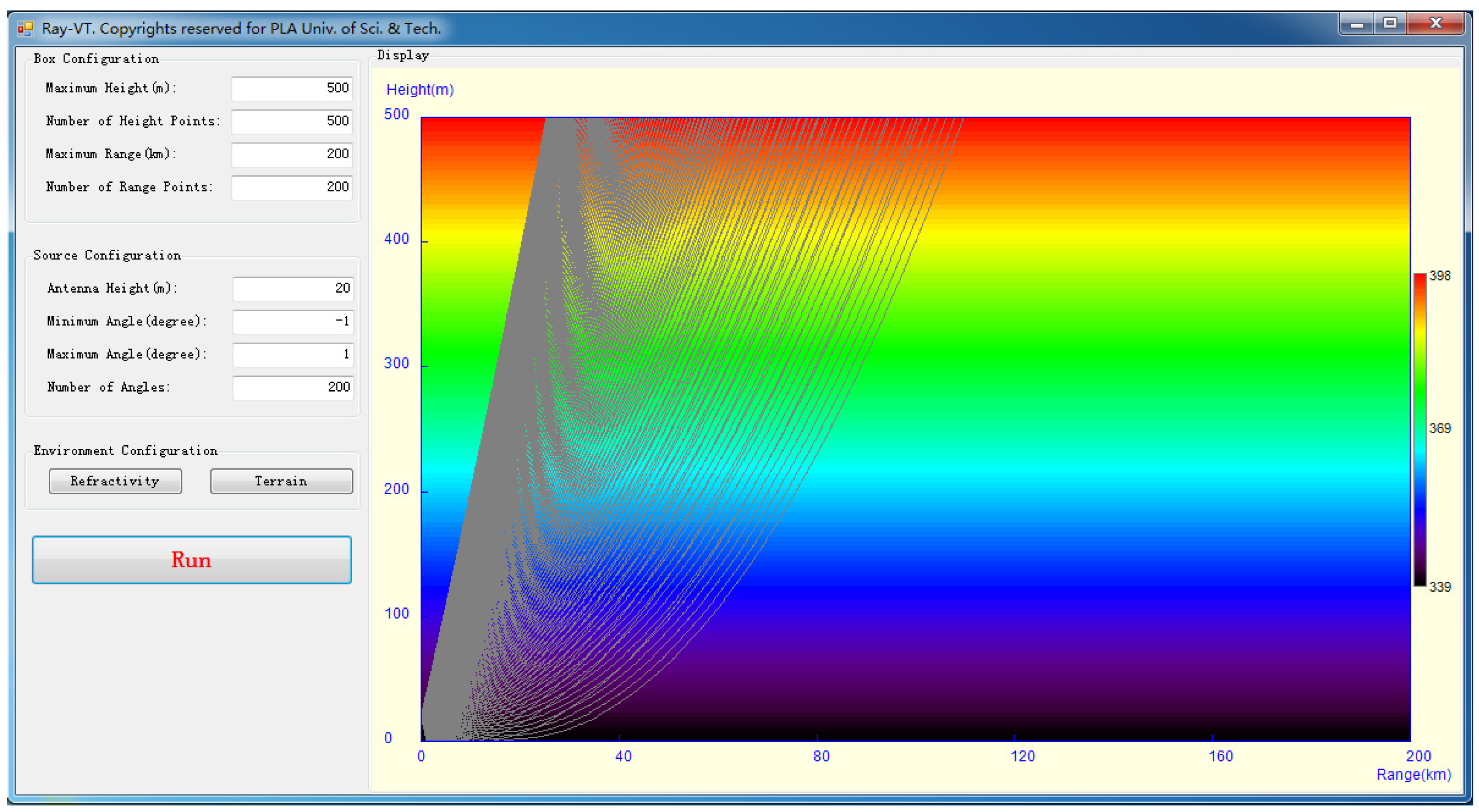
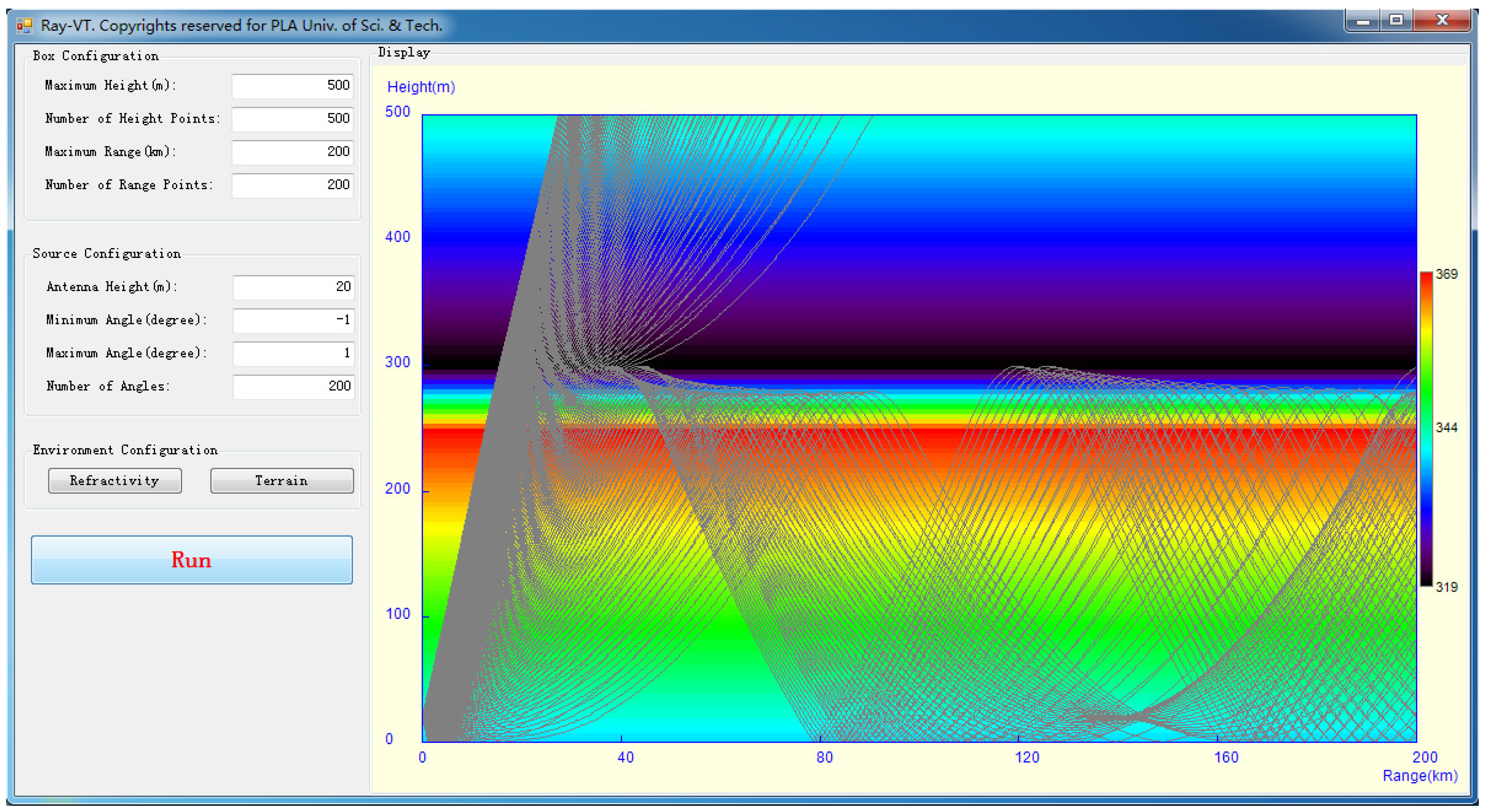
Figure 2, the front-end design of the Ray-VT is introduced. The graphical user interface (GUI) is divided into four parts: box configuration, source configuration, environment configuration and display window.
The box configuration contains the computation domain and the computation size, including the maximum height z max , the height points n z , the maximum range r max and the range points n r . Using these variables, the height bin z and range bin r are, respectively, determined as z = z max / n z and r = r max / n r . The values of these variables can be selected or changed by the user directly.
The source configuration contains the antenna height and the elevation angles. The ray paths are traced for a set of different elevation angles. The elevations are determined with the same interval ( θ max θ min ) / n θ , by the minimum angle θ min , the maximum angle θ max , and the angle numbers n θ . These values are also selected according to the user’s requirements.
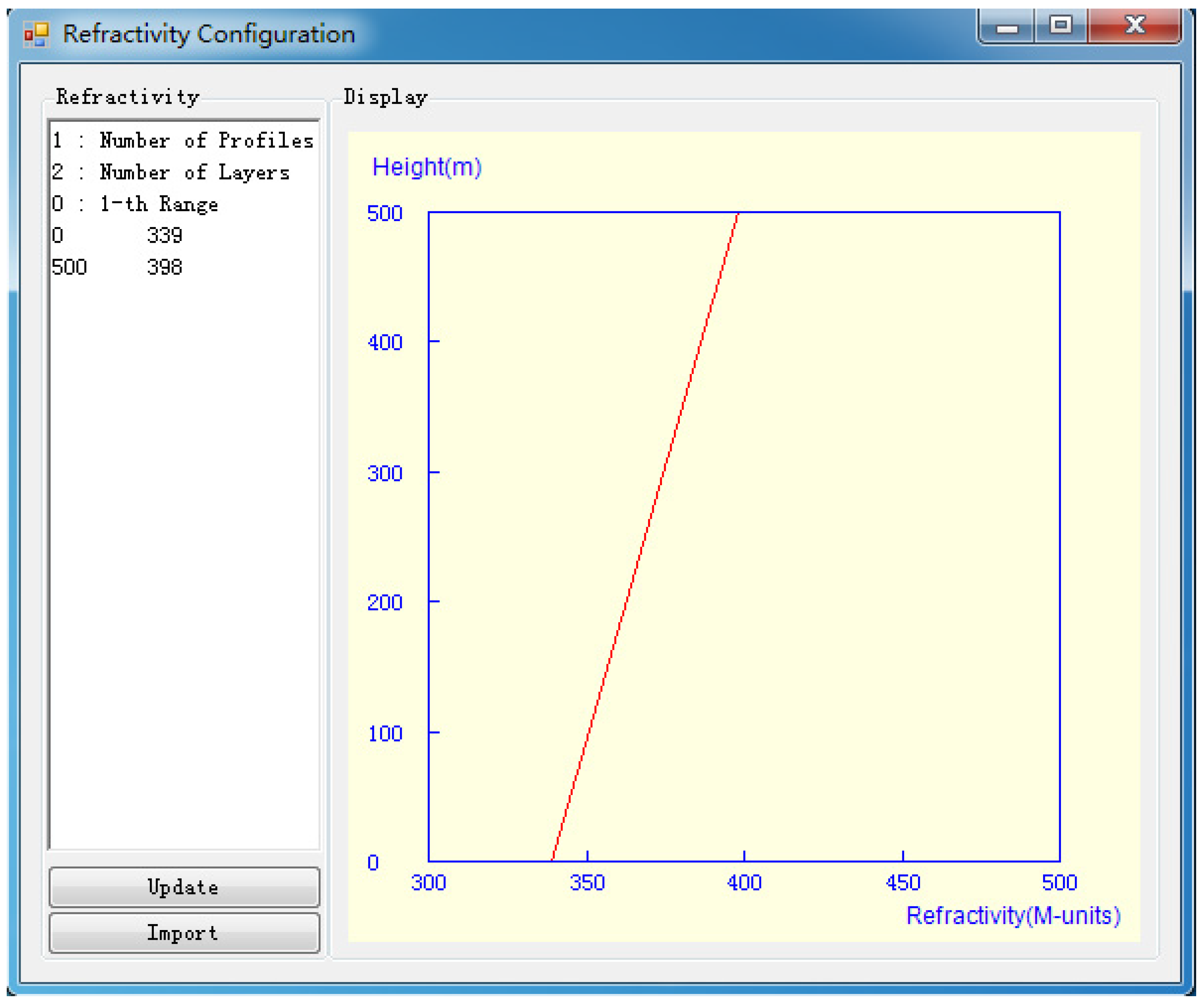
The environment configuration contains the refractivity and the terrain information, which are related to the “refractivity” and the “terrain” buttons. Figure 3 gives the GUI of the refractivity information. The refractivity profile can be imported from a preexisting text file or specified by the user in the left textbox. The right display window shows the modified refractivity M versus the height, where M = ( m 1 )   ×   10 6 . The terrain profile can be manipulated in the same manner (not shown).
The display window in Figure 2 shows the ray paths corresponding to a total of 200 rays emanating from a source located at a 20 m height. The maximum and the minimum elevation angles are 1° and −1°, respectively. The color contour shows the spatial variations of the refractivity with the limits given by the right colorbar. Here, the refractivity corresponds to a range-independent standard refractive environment as shown in Figure 3.
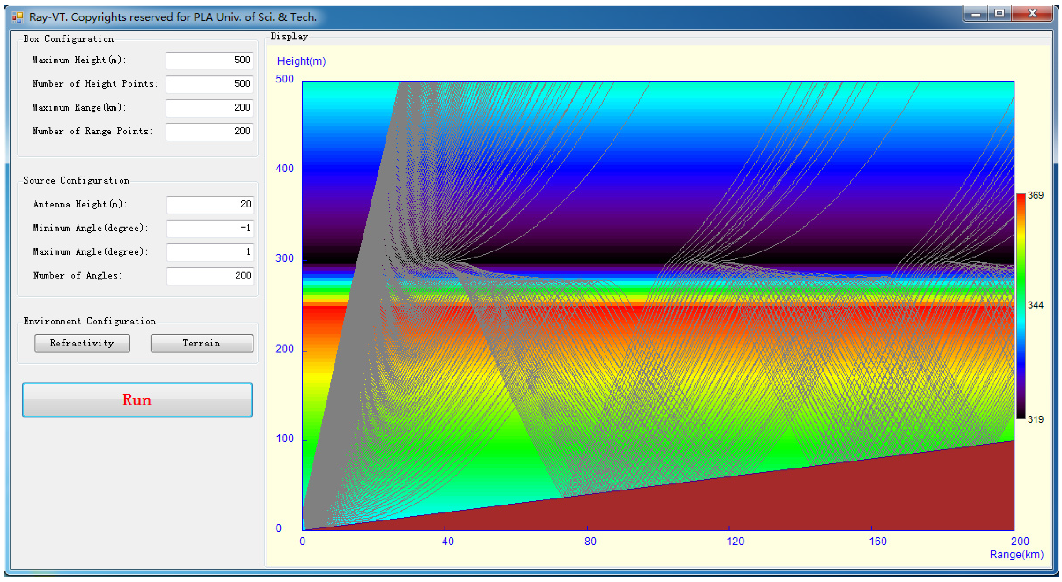
Figure 4 gives another propagation scenario with the refractivity profile characterized by a 300 m surface-based duct with a base height of 250 m, a thickness of 50 m, and a strength of 39.5 M-units. Here, it should be noted that in the atmospheric duct environment, there exists a critical trapping angle θ c which is determined by the difference between the minimum modified refractive index m min and the value at the antenna height m ant , i.e., θ c = ± 2 ( m ant m min ) . Here the critical trapping angle is 0.383°.
As can be seen in Figure 2 and Figure 4, the Ray-VT is an effective tool to investigate tropospheric refraction effects. In the standard atmosphere, the rays’ radius of curvature is larger than the Earth’s radius, and the rays flee away the Earth’s surface. In this case, the radar’s effective range (line-of-sight) is limited to within 30 km, while in the surface-based duct environment, most of the rays within the critical angle are trapped in the duct layer and travel over the horizon, and the radar-blind areas are also easily fixed. The ray trajectory predictions will be useful for determining the optimal positions for beyond line-of-sight communications.
Figure 5 gives the ray paths on a smooth wedge-shaped terrain for the 300 m surface-based duct environment. The bottom closed deep color shows the terrain profile. Comparing Figure 5 with Figure 4, along the propagation path, some captured rays are released to the upper space as a result of slope terrain reflections that change the reflection angles and make some of them go beyond the critical angle.
The above propagation scenarios are focused on range-independent refractivity, but their extension to range-dependent cases is straightforward. Owing to the fact that the spatial change of tropospheric refractivity is larger with height than with range, the horizontal homogeneity assumptions of the refractive environment in a local range are generally demonstrated to be reasonable [22,23]. Thus, for the range-dependent case, the refractivity can be assumed to be horizontally homogeneous in each ray-tracing step (say tens or hundreds of meters) and updated at different tracing steps.
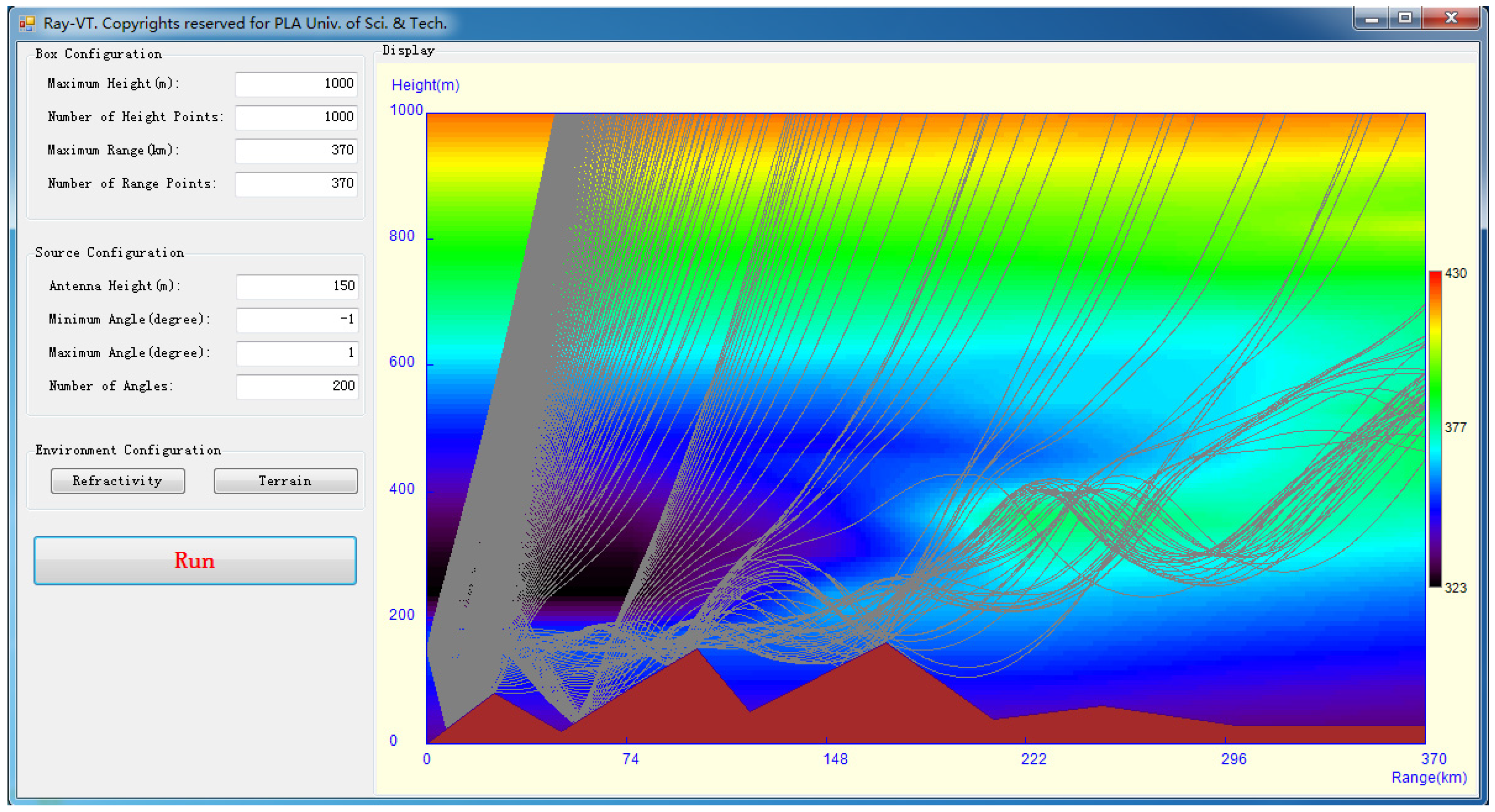
A propagation scenario for the range-dependent refractive conditions with a much more complex terrain is shown in Figure 6. The high resolution refractivity field, corresponding to a Pt. Loma to Guadalupe Island transect of 12 March 1948, is used [20]. The data consist of five M-units versus height profiles, at ranges of 0, 148, 222, 296 and 370 km. Before the tracing process, the refractivity data are manipulated by the method shown in Section 2.2. The source height for this scenario is 150 m, and 200 rays limited between −1° and 1° elevation angles are used. It is clear from the background color contour in Figure 6 that the trapping layer increases slowly from 0 to 370 km, where the duct gradually evolves from the surface-based duct to elevated duct. Owing to the duct propagation, the rays limited to the critical angle are mainly captured in the duct layer.

4. Accuracy Validation

The Ray-VT tool is just designed to draw ray paths through a complex environment, and the EM field contributions of rays are not considered. How to use the ray-tracing method to calculate the EM field values is explained in [24], but this method usually fails at focal points and caustics. For EM field calculations, the full-wave methods, for example the PE method, will provide more accurate results. Owing to the field strength having a strong correlation with the ray density [25], the PE method can be used to validate the accuracy of Ray-VT indirectly. In this paper, the TPEM propagation model [10] is used.
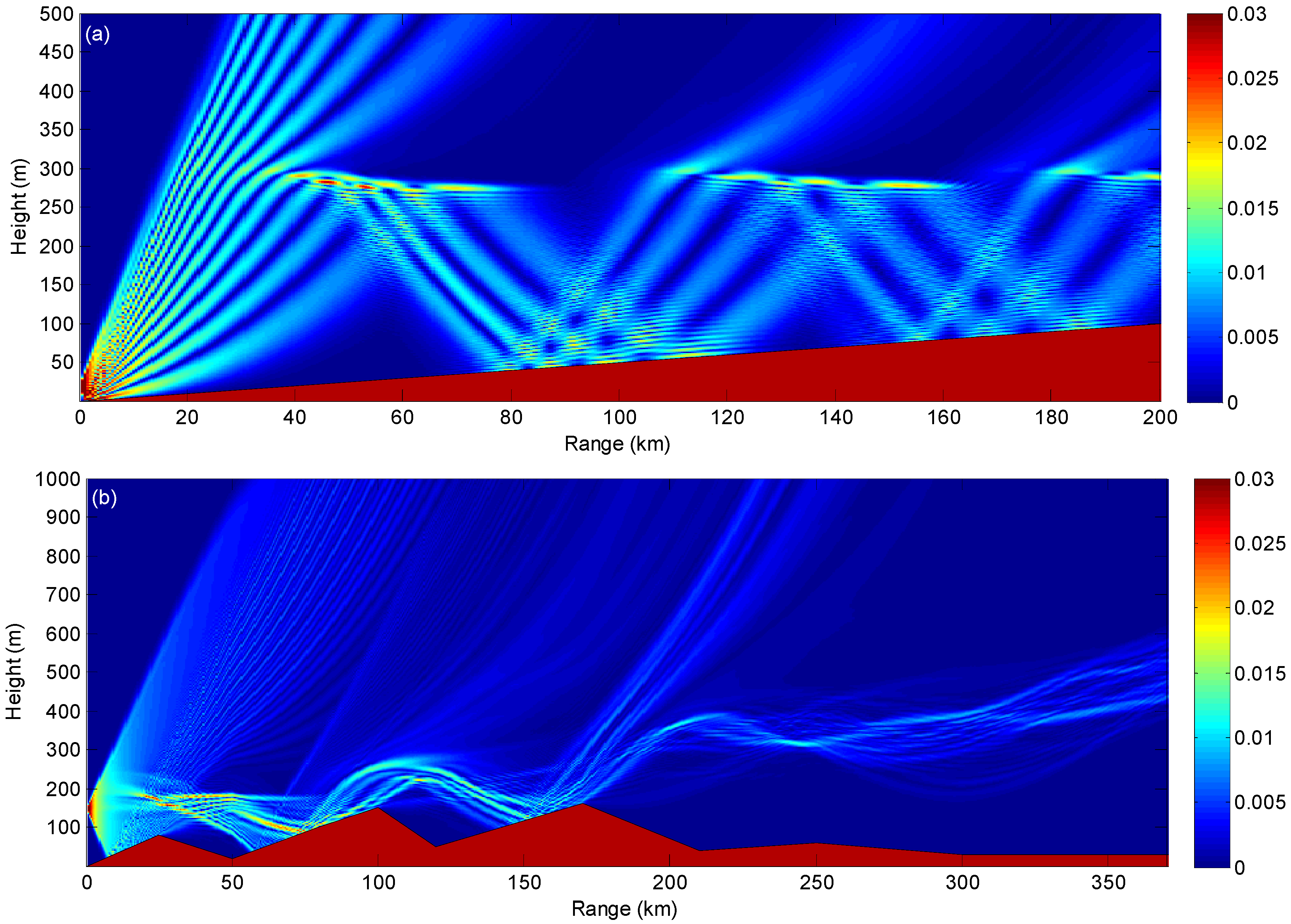
Figure 7 gives the coverage diagrams of the field strength computed by TPEM, where the antenna source is assumed to be omnidirectional and horizontally polarized with a frequency of 5 GHz. The environmental information in Figure 7a,b corresponds to that in Figure 5 and Figure 6, respectively.
As can be seen in Figure 7a, due to the existence of the atmospheric duct, most of the EM energy is trapped in the duct layer, and the field strength distributions are in good agreement with the ray paths shown in Figure 5. Besides, the energy leakage above the duct at ranges of 110 km and 180 km agrees very well with the released rays at the same ranges. Perfect agreement can also be found by comparing Figure 6 with Figure 7b, which indicates that the Ray-VT can predict the ray paths in the complex range-dependent environment, both of refractivity and terrain, in a sophisticated manner.
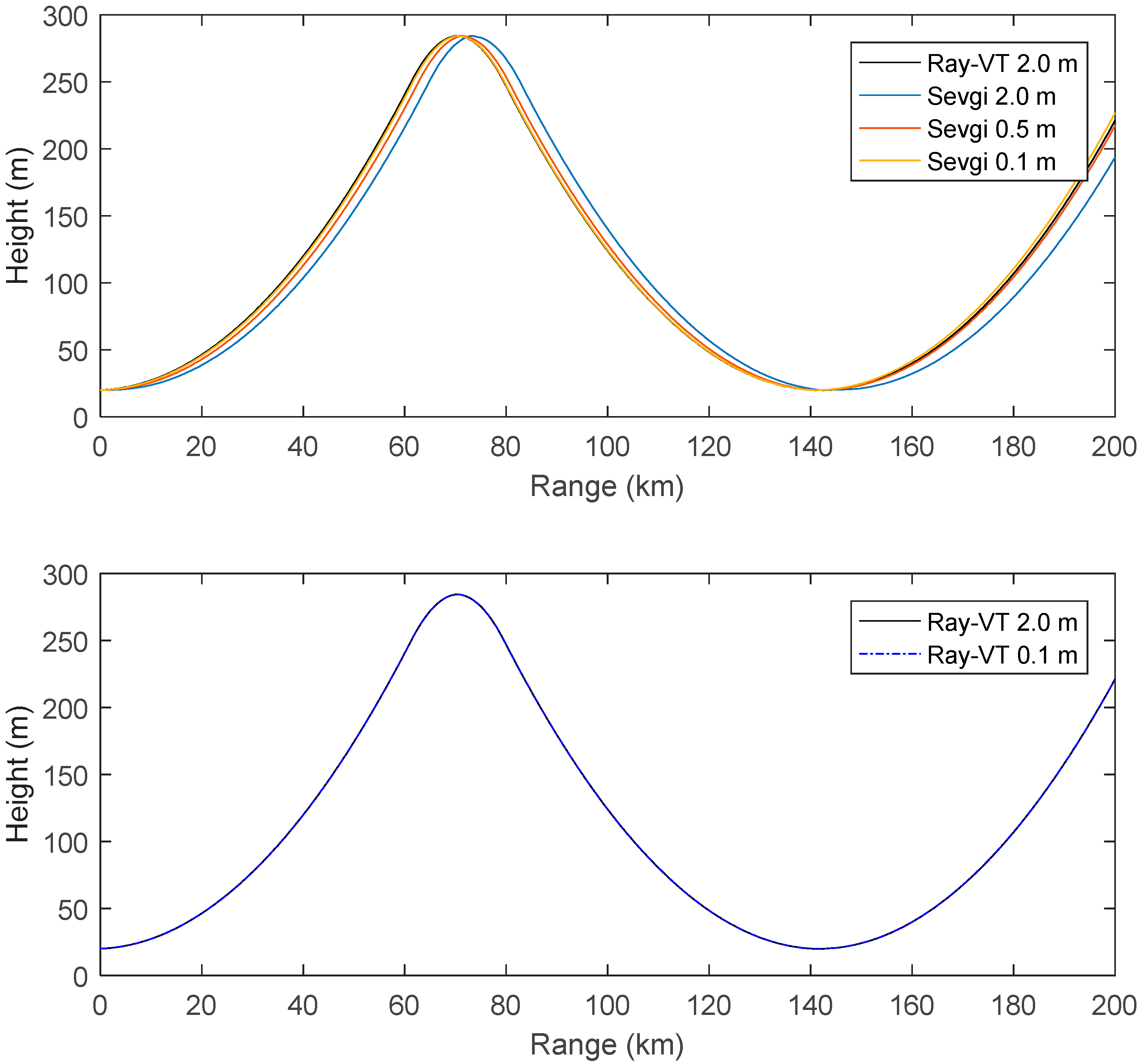
Figure 8 compares the ray paths between the Ray-VT and Sevgi’s tool [15] for surface-based duct propagation with an elevation angle of 0.01°, in which the vertical intervals for the Ray-TV were set at 2 m and 0.1 m, respectively, and the vertical intervals for Sevgi’s tool were set at 2 m, 0.5 m, and 0.1 m, respectively. It is clear seen that there are some differences in the ray trajectories of Sevgi’s tool for different vertical intervals, shown in Figure 8a, where the height difference at the range of 200 km for 2 m and 0.1 m vertical intervals reaches 33.1 m. This phenomenon for Sevgi’s tool originates from the constant refractive index assumption between adjacent vertical layers. Although a smaller interval can obtain a more accurate result, the computation time will be increased at the same time. In the Ray-VT, the gradient of the refractive index layer is considered, which makes the ray path computation for different vertical intervals more stable, as shown in Figure 8b where the ray paths of the Ray-VT overlap very well for the vertical intervals of 0.1 m and 2 m. In Figure 8a, the ray path of the Ray-VT matches well with the ray path of Sevgi’s tool with a 0.1 vertical interval, and the average height difference along the propagation range is only 0.38 m. In this case, the Ray-VT just needs near one-twentieth of computation time of Sevgi’s tool.
Here, it should be noted that the validity of the small angle approximation must guarantee the shooting angle is relatively small (less than one degree). Otherwise, the error will be brought by the Taylor approximation of large angles. On the other hand, the Ray-VT uses the vertical gradient information of the refractivity. So, it should guarantee that the gradient at a fixed layer does not change.

5. Conclusions

A simple ray-tracing visual tool, Ray-VT, has been designed and introduced in this paper. The necessary input parameters can be specified in the interactive window directly. The tool can accurately simulate the ray paths in a heterogeneous atmospheric medium over variable terrain, which has good agreement with the field strength distributions computed by the PE method. The Ray-VT can be used as an engineering tool to investigate the effects of ducting propagations and to assess the performances of radar systems, such as predicting the radar’s effective range and radar-blind areas, and determining the optimal positions for beyond line-of-sight communications in the duct environment. It can also be used as an educational aid in EM lectures, for example in antennas and propagation, wireless communication, etc., for understanding the propagation characteristics in complex environments.

Acknowledgments

This work was supported by the National Natural Science Foundation of China (41405025), and Jiangsu Province Natural Science Foundation of China (BK20140064). The Ray-VT can be downloaded at the link http://pan.baidu.com/s/1gdAFB9p.

Author Contributions

Xiaofeng Zhao conceived and designed the method; Xiaofeng Zhao and Pinglv Yang performed the experiments and wrote the paper.

Conflicts of Interest

The authors declare no conflict of interest.

References

  1. Oka, E. Ray-tracing analysis of anomalous propagation through horizontally nonuniform surface duct. Electr. Commun. Jpn. 1991, 74, 79–87. [Google Scholar] [CrossRef]
  2. Akbarpour, R.; Webster, A.R. Ray-tracing and parabolic equation methods in the modeling of a tropospheric microwave link. IEEE Trans. Antennas Propagat. 2005, 53, 3785–3791. [Google Scholar] [CrossRef]
  3. Gegout, P.; Oberle, P.; Desjardins, C.; Moyard, J. Ray-tracing of GNSS signal through the atmosphere powered by CUDA, HMPP and GPUs technologies. IEEE J.-STARS 2014, 7, 1592–1602. [Google Scholar] [CrossRef]
  4. Kunz, G.J.; Moerman, M.M.; van Eijk, A.M.J. ARTEAM: Advanced ray tracing with earth atmospheric models. SPIE Proc. 2002, 4718, 397–404. [Google Scholar]
  5. Kunz, G.J.; Moerman, M.M.; van Eijk, A.M.J.; Hammel, S.M.; Tsintikidis, D. EOSTAR: An electro-optical sensor performance model for predicting atmospheric refraction, turbulence and transmission in the marine surface layer. SPIE Proc. 2004, 5237, 81–92. [Google Scholar]
  6. Nafisi, V.; Urquhart, L.; Santos, M.; Nievinski, F.; Boehm, J.; Wijaya, D.; Schuh, H.; Ardalan, A.; Hobiger, T.; Ichikawa, R.; et al. Comparison of ray-tracing packages for troposphere delays. IEEE Trans. Geosci. Remote Sens. 2012, 50, 469–481. [Google Scholar] [CrossRef]
  7. Van Eijk, A.M.J.; Kunz, G.J. The introduction of horizontal inhomogeneity of meteorological conditions in the EOSTAR propagation model. SPIE Proc. 2006, 6303. [Google Scholar] [CrossRef]
  8. Dockery, G.D. Modeling electromagnetic wave propagation in the troposphere using the parabolic equation. IEEE Trans. Antennas Propagat. 1988, 36, 1464–1470. [Google Scholar] [CrossRef]
  9. Kuttler, J.R.; Dockery, G.D. Theoretical description of the parabolic approximation/Fourier split-step method of representing electromagnetic propagation in the troposphere. Radio Sci. 1991, 26, 381–393. [Google Scholar] [CrossRef]
  10. Barrios, A. A terrain parabolic equation model for propagation in the troposphere. IEEE Trans. Antennas Propagat. 1994, 42, 90–98. [Google Scholar] [CrossRef]
  11. Ozgun, O.; Apaydin, G.; Kuzuoglu, M.; Sevgi, L. PETOOL: MATLAB-based one-way and two-way split-step parabolic equation tool for radiowave propagation over variable terrain. Comput. Phys. Commun. 2011, 182, 2638–2654. [Google Scholar] [CrossRef]
  12. Sevgi, L. A mixed-path groundwave field-strength prediction virtual tool for digital radio broadcast systems in medium and short wave bands. IEEE Antenn. Propag. Mag. 2006, 48, 19–27. [Google Scholar] [CrossRef]
  13. Sevgi, L. Groundwave modeling and simulation strategies and path loss prediction virtual tools. IEEE Trans. Antennas Propagat. 2007, 55, 1591–1598. [Google Scholar] [CrossRef]
  14. Sevgi, L. A new electromagnetic engineering program and teaching via virtual tools. Prog. Electromagn. Res. B 2008, 6, 205–224. [Google Scholar] [CrossRef]
  15. Sevgi, L. A ray-shooting visualization Matlab package for 2D ground-wave propagation simulations. IEEE Antenn. Propag. Mag. 2004, 46, 140–145. [Google Scholar] [CrossRef]
  16. Hattan, C.P. A Ray Trace Model for Propagation Loss; Technical Report 1576; NCCOSC: San Diego, CA, USA, 1993. [Google Scholar]
  17. Hitney, H.V. Hybrid ray optics and parabolic equation methods for radar propagation modelling. In Proceedings of the International Conference on Radar, Brighton, UK, 12–13 October 1992.
  18. Barrios, A. Considerations in the development of the advanced propagation model (APM) for U.S. Navy applications. In Proceedings of the International Conference on Radar, Adelaide, Australia, 3–5 September 2003.
  19. Yan, H.J.; Fu, Y.; Hong, Z.J. Introduction to Modern Atmospheric Refraction; Science and Educational Press: Shanghai, China, 2006. (In Chinese) [Google Scholar]
  20. Vogel, G.N. Specification for a Refractivity Structure Matching Algorithm; Final Report; Naval Oceanographic and Atmospheric Research Lab: Monterey, CA, USA, 1992. [Google Scholar]
  21. Jensen, F.B.; Kuperman, W.A.; Porter, M.B.; Schmidt, H. Computational Ocean Acoustics, 2nd ed.; Springer: Berlin, Germany, 2011. [Google Scholar]
  22. Hitney, H.V.; Richter, J.H.; Pappert, R.A.; Anderson, K.D.; Baumgartner, G.B. Tropospheric radio propagation assessment. Proc. IEEE 1985, 73, 265–283. [Google Scholar] [CrossRef]
  23. Goldhirsh, J.; Dockery, D. Propagation factor errors due to the assumption of lateral homogeneity. Radio Sci. 1998, 33, 239–249. [Google Scholar] [CrossRef]
  24. Valtr, P.; Pechac, P. Analytic tropospheric ray-tracing model for constant refractivity gradient profiles. In Proceedings of the First European Conference on Antennas and Propagation, Nice, France, 6–10 November 2006.
  25. Barrios, A. Estimation of surface-based duct parameters from surface clutter using a ray trace approach. Radio Sci. 2004, 39. [Google Scholar] [CrossRef]
Figure 1. The sketch map of ray tracing for one tracing step.
Atmosphere 08 00035 g001
Figure 2. GUI (graphical user interface) of the Ray-VT for rays propagating through a standard refractive environment on a flat terrain.
Atmosphere 08 00035 g002
Figure 3. GUI of refractivity information.
Atmosphere 08 00035 g003
Figure 4. GUI of the Ray-VT for rays propagating through a 300 m surface-based duct on a flat terrain.
Atmosphere 08 00035 g004
Figure 5. GUI of the Ray-VT for rays propagating through a 300 m surface-based duct on a smooth wedge-shaped terrain.
Atmosphere 08 00035 g005
Figure 6. GUI of the Ray-VT for rays propagating through the refractivity fields measured between a Pt. Loma and Guadalupe Island of 12 March 1948.
Atmosphere 08 00035 g006
Figure 7. The coverage diagrams of the field strength computed by TPEM, (a) for a range-independent 300 m surface-based duct environment; and (b) for a range-dependent refractive environment measured between Pt. Loma and Guadalupe Island on 12 March 1948.
Atmosphere 08 00035 g007
Figure 8. Comparison of the ray paths between the Ray-VT and Sevgi’s tool for the surface-based duct propagation with elevation angle of 0.01°.
Atmosphere 08 00035 g008

