Article

A Case Study of Assimilating Lightning-Proxy Relative Humidity with WRF-3DVAR

1
Key Laboratory of Arid Climatic Changing and Reducing Disaster of Gansu Province, College of Atmospheric Sciences, Lanzhou University, No.222 TianShui South Road, Lanzhou 730000, China
2
Key Laboratory of Middle Atmosphere and Global Environment Observation (LAGEO), Institute of Atmospheric and Physics, Beijing 100029, China
3
National Meteorological Information Centre, China Meteorological Administration, Beijing 100081, China
4
Chinese Academy of Meteorological Sciences, Beijing 100081, China
*
Author to whom correspondence should be addressed.
Atmosphere 2017, 8(3), 55; https://doi.org/10.3390/atmos8030055
Submission received: 4 January 2017 / Revised: 9 March 2017 / Accepted: 11 March 2017 / Published: 14 March 2017
(This article belongs to the Section Meteorology)

Abstract

:
Lightning network data, considered as a useful supplement to radar observations, are a good indicator of severe convection, and has high temporal and spatial resolution. In Numerical Weather Prediction (NWP) models, lightning data are a new source of data to improve the forecasting of convective systems. In this case study, lightning data assimilation is conducted by converting lightning data to water vapor mixing ratio via a simple smooth continuous function, with input variables of total flash rate and simulated graupel mixing ratio at 9 km gridded resolution. Relative humidity converted from the retrieved water vapor mixing ratio is assimilated into the background field utilizing the three-dimensional variational (3DVAR) method in WRFDA (the Weather Research and Forecasting model Data Assimilation system). The benefits of assimilating lightning data are demonstrated in a series of experiments using data from a strong convection event that affected Beijing, Tianjin, Hebei and Shandong Province, on 31 July 2007. A nested domain with resolutions of 9 km and 3 km is implemented. For this case, assimilating lightning data shows some improvements in predictions of both reflectivity and neighboring precipitation, and in the temperature, dew-point temperature and relative humidity profile after seven hours.

1. Introduction

Lightning is a common discharge phenomenon in convective weather. Electric charges are carried by ions and hydrometeors. It is well established that the non-inductive process is the dominant electrification mechanism in convective clouds [1,2]. In the supercooled environment in convective clouds, small ice crystals grow owing to vapor diffusion and accretion of supercooled water droplets. During elastic collisions between more or less rimed particles in the supercooled environment, charges are exchanged between the colliding particles. As the non-inductive process occupies the leading role, charges of opposite polarities separate in rebounding collisions between growing graupel pellets. Charges are then separated at the cloud scale by sedimentation, and vertical motions. The strong relationship among lightning, cloud dynamics and microphysical processes means that lightning can be used to monitor the occurrence and development of mesoscale convective systems [3,4,5,6]. Under the influence of thermodynamics, dynamics, or terrain, an ascending air mass can form thunderstorm clouds in a convectively unstable environment. Inside the thunderstorm clouds, hydrometeors with different velocities continually collide and separate. Charge transfer results in hydrometeors carrying electric charges of different polarity, and lightning occurs as a result of the accumulation of these electric charges. Therefore, lightning is an outcome of sufficiently severe convection.
Lightning network data are a new type of observation in meteorology and their application and investigation are subjects of current research. Lightning data are relatively unaffected by geographical constraints, and are available at higher temporal and spatial resolution than meteorological radar observations. Lightning data assimilation is a key topic in contemporary research. The difficulty is that lightning flash rate, electric field and charge density are not modeled or prognostic variables in most existing models. Hence, the concept of assimilating lightning data is to find a suitable observation operator that links lightning network data with a model or diagnosed variable, or to obtain a proper lightning data proxy which is physically sound, and then to use different methods to assimilate this variable. In past decades, many researchers have tried to find a reliable relationship between lightning data and other meteorological variables based on the microphysical mechanism in convective clouds, such as convective precipitation rate [7,8,9,10], convective available potential energy (CAPE) [11,12], maximum vertical velocity [13], proxy radar reflectivity [14,15,16,17], graupel mass [18], ice mass flux product [19,20], and updraft volume [21,22].
Several methods have been used to assimilate lightning data. Alexander et al. [23] demonstrated the benefit of lightning data assimilation. They combined lightning flash observations together with a classic image processing technique to achieve a continuous time series of rain rate, which is challenging over data-sparse regions. Their results show that the lightning data have a greater positive impact on forecasts than that from passive microwave sensors and infrared sensors. Chang et al. [24] also confirmed that using lightning as a continuous proxy can improve weather forecasts. A different approach used by some researchers is to transform lightning data into convective precipitation rate and then adjust the latent heat profile by nudging. Papadopoulos et al. [25] used cloud-to-ground lightning data to nudge model-generated humidity profiles towards empirical profiles. Their results show that assimilation of lightning data can significantly improve the prediction of convective precipitation up to 12 h ahead. Stefanescu et al. [11] treated convective available potential energy as a proxy for lightning data. They selected 1D + nD-VAR (one dimensional + n dimensional variational) (n = 3, 4) method to assimilate ENTLN (the Earth Networks Total Lightning Network) lightning data and evaluated its performance in two severe storm cases. 1D-VAR technique was firstly utilized to obtain temperature increments, which were then added into the background to achieve column temperature retrievals. The column temperature retrievals were then associated with observed lightning data and assimilated into the WRFDA (the Weather Research and Forecasting model Data Assimilation system) nD-VAR (n = 3, 4) framework as conventional data. The results showed that the best improvement was with the 1D + 4D-VAR technique, which decreased the precipitation root mean square errors in both case studies. Qie et al. [26] utilized an empirical formula from Fierro et al. [27] and substituted the water vapor mixing ratio with the ice-phase mixing ratio to connect total lightning flash rate with ice-phase particles. They then added the nudging function into the WSM6 (the WRF Single-Moment 6-Class) microphysical scheme of the WRF (the Weather Research and Forecasting model)to adjust the mixing ratio of ice-phase particles between the 0 °C and −20 °C isotherms. They found that this method could be used for improving the short-term precipitation forecasting of Mesoscale Convective Systems (MCSs) with high or moderate lightning flash rates. However, adding ice-phase particles in severe convective regions may augment the vertical downdraft that would be an obstacle for the lateral development of convective systems. Thus, their scheme may perform poorly when applied to a wide range of thunderstorm cases. Some researchers have tried treating lightning as an index to control parameterization schemes. Gallus and Segal [28] used the National Centers for Environmental Prediction (NCEP) Eta Model with a 10 km horizontal grid spacing to simulate 20 MCS cases. They found that adding humidity information in regions where the radar echo is high with low humidity can improve forecasting skill, and that the Kain–Fritsch (KF) parameterization scheme performs better than the Betts–Miller–Janjic (BMJ) parameterization in a cold pool. Mansell et al. [29] tested the effect of lightning data assimilation on KF cumulus parameterization in a Coupled Ocean–Atmosphere Mesoscale Prediction System. They utilized lightning as an index to control the KF parameterization scheme for the presence or absence of deep convection. With this method, the lightning data assimilation was successful in generating cold pools that were present in surface observations at forecast initialization, and the improvement was obvious in the first few hours. Lightning data were also utilized as a proxy to control the activation of the convective parameterization scheme in the MM5 (Mesoscale Model 5) non-hydrostatic model by Lagouvardos et al. [30]. The assimilation of lightning was shown to have a positive impact on the representation of the precipitation field, and provided more realistic positioning of precipitation maxima, mainly during the second day of the event. Mansell [31] designed a set of observing system simulation experiments to demonstrate the potential benefit of assimilating total lightning flash mapping data using the ensemble Kalman filter (EnKF) method. In his assimilation algorithm, a linear relationship between flash rate and graupel echo volume was utilized as the observation operator. In Rapid Refresh, which is the continental-scale National Oceanic and Atmospheric Administration (NOAA) hourly-updated assimilation/modeling system operational at NCEP, lightning data are considered a good supplement to radar data to improve convective coverage off the coast. In this system, lightning data are transformed into proxy radar reflectivity, which is then assimilated into the numerical weather prediction (NWP) model [14,15,16,17].
In our previous work, we attempted to assimilate lightning data utilizing radar proxy reflectivity transformed in Gridpoint Statistical Interpolation (GSI) code using diverse methods such as physical initialization and cloud analysis [32,33,34]. However, each method had shortcomings; for example, cloud analysis provided stronger precipitation in short-term forecasts after assimilation than was observed [33]. The physical initialization method provided a better precipitation forecast, but the improvement was short-lived [32]. These limitations provide motivation for an improved scheme for linking lightning data with other variables. Fierro et al. [27] suggested a simple relationship between flash rate and the water vapor mixing ratio at 9 km resolution that appears useful. In their case study, the nudging method was used primarily for analysis rather than forecast. This simple and computationally inexpensive assimilation technique can be easily implemented into the WRF model and showed promising improvements in the representation of the convection and cold pools at the analysis time to provide more accurate analysis and forecasts of storm structure and evolution. Marchand and Fuelberg [35] put forward a method that warmed the most unstable low levels of the atmosphere at locations where lightning was observed but deep convection was not simulated due to the absence of graupel. They compared their simulation results with the Fierro et al. [27] nudging method. The new method performed better at simulating isolated thunderstorms and other weakly forced deep convection, while the Fierro et al. [27] nudging method performed better for cases with strong synoptic forcing. In Fierro et al. [36], the smooth nudging method was also compared with a three-dimensional variational (3DVAR) technique which assimilated radar reflectivity and radial velocity data. A suite of sensitivity experiments revealed that lightning assimilation was better able to capture the position and intensity of reflectivity up to 6 h into the forecast. The computationally inexpensive lightning data nudging method was evaluated with more case studies in Fierro et al. [37]. The performance of the accumulated precipitation forecast for 67 days in the 2013 USA warm season was evaluated. The results showed that the nudging method had considerable promise for routinely improving short-term (≤6 h) forecasts of high-impact weather with convection-allowing forecast models. The Fierro et al. [27] nudging method is efficient for initializing convection where lightning is detected, but has limited ability to suppress spurious convection or to modulate convection.
Nudging is a type of economical four-dimensional data assimilation method. The advantage of the nudging method is that it can incorporate assimilated data at proper time even at several integration steps. It relaxes the model state to the observations during the assimilation period by adding a non-physical diffusive-type term to the model equations [38]. However, the approach is only a fitting procedure between observed data and model variables and lacks a solid theoretical foundation; it does not consider physical process and physical balances between analyzed variables. In variational methods, 3DVAR and 4DVAR are widely used in many operational platforms. The 3DVAR method is popular as it has a high computational efficiency and can directly assimilate various observations (e.g., conventional data, radar data, bogus data, etc.). The basic concepts of 3DVAR and 4DVAR methods are the same except that the 4DVAR method employs an additional set of prognostic equations as a strong constraint [39,40]. The 4DVAR method utilizes an optimal control approach based on the adjoint model integration process to obtain the gradient of the cost function, with respect to the control variables for the minimization procedure [38]. One difference between 3DVAR and 4DVAR is the background error covariance. The 3DVAR framework utilizes a static background error covariance, while in the 4DVAR framework, the background error covariance varies with flow patterns, which may achieve a more detailed analyzed field. Nevertheless, calculating adjoint with high resolution in a 4DVAR framework needs great computational power, which is not available in some real-time operational platforms. As lightning data are a good supplement to radar data, using the 3DVAR method to assimilate lightning data can easily be implemented in many existing operational model platforms, which utilize the same method to assimilate radar data and conventional data for daily real time forecasts. Thus, in this study, a 3DVAR method that can adjust variables within an influence radius is used in the assimilation of total lightning data, and is tested based on the relationship between total flash rate and water vapor.
Based on a large number of case studies tested in Fierro et al. [37], the lightning data assimilation algorithm in this paper converts lightning data to water vapor mixing ratio via the simple smooth continuous function given in Fierro et al. [27]. In their study, a9 km gridded resolution total flash rate and simulated graupel mixing ratio were used as input variables. The water vapor mixing ratio is then transformed into relative humidity in the form of sounding data. Finally, the proxy relative humidity is assimilated into the background field utilizing the 3DVAR method in WRFDA. The benefits of assimilating lightning data are demonstrated in a series of experiments using data from a strong convection event that affected Beijing, Tianjin, Hebei and Shandong Province, on 31 July 2007. The remainder of this paper is organized as follows. Section 2 describes the methodology, Section 3 presents results and discussion, and Section 4 summarizes the findings.

2. Methodology

2.1. Assimilation Algorithm

Fierro et al. [27] suggested a simple smooth continuous equation that gives the water vapor mixing ratio in terms of the flash rate and the simulated graupel mixing ratio:
Q v = A Q s a t + B Q s a t tanh ( C X ) [ 1 tanh ( D Q g α ) ]
where X is the total number of flashes per 10 min, Q s a t is the water vapor saturation mixing ratio, and Q g is the graupel mixing ratio (g·kg−1). Water vapor is modified in the mixed-phase region between the 0 °C and −20 °C isotherms, where electrification of ice and water produces electric charges and is the region mostly associated with the occurrence of lightning. Values for coefficients A , B , C , D and α were set as 0.81, 0.2, 0.01, 0.25, and 2.2, respectively, based on many case studies from Fierro et al. [37]. The variation of Q g with observed total flashes is shown in Figure 7 of Fierro et al. [27]. The water vapor obtained from the formula was transformed it into relative humidity in the form of sounding data, for use in the WRFDA-3DVAR.
The 3DVAR method is one of the variational data assimilation algorithms available in WRFDA. It aims to provide an improved estimate of the first guess through iterative minimization of a prescribed cost function:
J ( x ) = 1 2 [ ( x x b ) T B 1 ( x x b ) + ( H ( x ) y 0 ) T O 1 ( H ( x ) y 0 ) ]
where B is the background error covariance, O is the observation error covariance, and H is the observation operator. The background error covariance typically sets the time-invariant component in the 3DVAR method. Thus, the background error covariance B used in our case study was the statistic CV5 (control variables option 5) BE (background error) derived within the same domain, to achieve a better encapsulated fixed climatology. The statistic CV5 option background error is computed using the NMC (National Meteorological Center) method [41] with the same WRF configuration as the case study.
The WRFDA-3DVAR system can directly assimilate radar reflectivity and radar radial velocity. It assimilates observed reflectivity utilizing a reflectivity operator to convert the model rainwater mixing ratio into reflectivity. A meaningful forecast rainwater field is hard to obtained with the statistic background error covariance [39]. Thus, the total mixing ratio q t is utilized as the moist control variable [42]. During the 3DVAR minimization, warm-rain microphysical processes are used to partition total mixing ratio q t increment into water vapor mixing ratio q v , cloud water mixing ratio q c and rainwater mixing ratio q r increments. Radar reflectivity is related to the rainwater mixing ratio using the Z-R relationship of Sun and Crook [43]:
Z = 43.1 + 17.5 log ( ρ q r )
where Z is radar reflectivity, ρ is air density and q r is rainwater mixing ratio.
The observation operator of radar radial velocity is [43]:
V r , i = u x x i r i + v y y i r i + ( w V T m ) z z i r i
where V T m is the terminal velocity of precipitation, ( u , v , w ) is the three-dimensional wind field, ( x , y , z ) is the Doppler radar location, ( x i , y i , z i ) is the Doppler radar observed target location and r i is the distance between observed point and radar location.

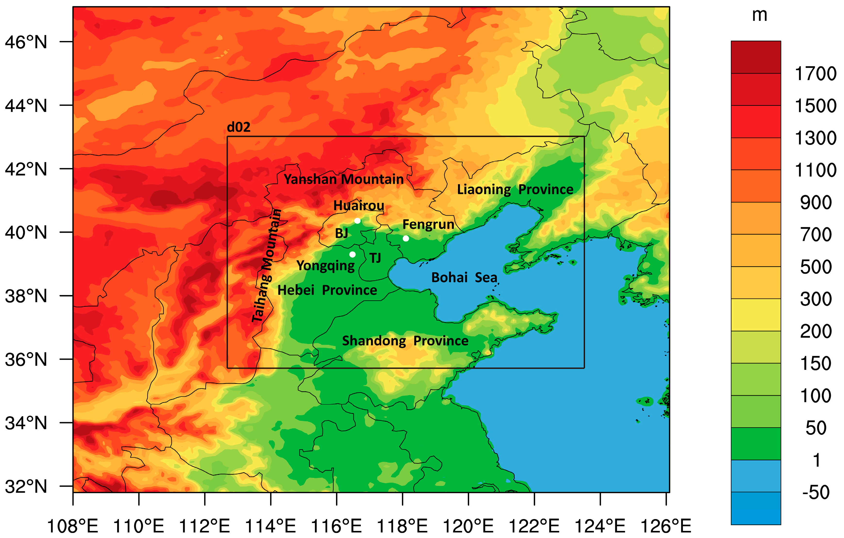
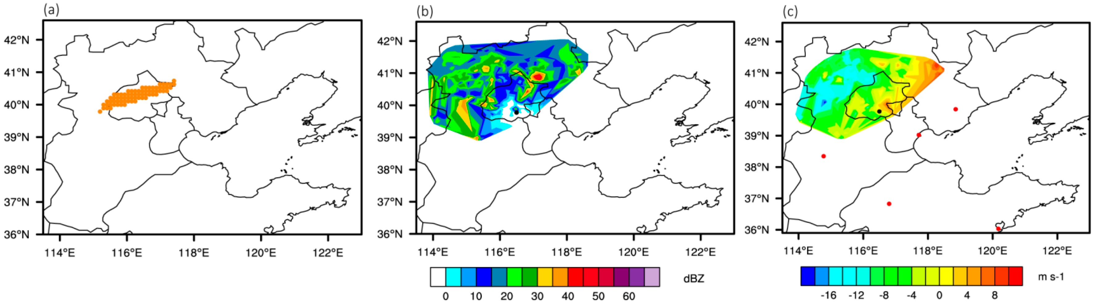
2.2. Data, Model Configuration and Experiment Design

The lightning data used in this study are from the SAFIR (Surveillance et Alerte Foudre par Interferometrie Radiometrique) 3000 lightning location system in Beijing, which includes three observation sites at Yongqing, Huairou, and Fengrun. The locations of these three sites are marked with white dots in Figure 1 (Huairou locates at 116.63° N, 40.36° E, Yongqing locates at 116.48° N, 39.30° E, and Fengrun locates at 118.10° N, 39.80° E). SAFIR has been widely used in Europe and Japan since the 1990s. The main measurement principle of the SAFIR system is to fix the direction of lightning with VHF (Very High Frequency) interference and then to pinpoint its location using results from sites. The VHF interference method differs from the TOA (Time of Arrival) method that is utilized in many existing lightning detection network (e.g., WWLLN (Worldwide Lightning Location Network)). The azimuth of the incoming wave with respect to the antenna array is determined by the phase difference of the signal received by the receiving antenna oscillator by the VHF interference method. Theoretically, with the VHF interference method, two detection sites are sufficient to complete the task of measuring lightning of the whole network and to control positioning error within 1 km. In the available detection region, positioning accuracy can reach 500 m and the detection efficiency of intra-cloud and cloud-to-ground flashesis higher than 95% (90% at 200 km, 80% at 250 km, and 60% at 270 km). The detection accuracy is less than 100 μs and a wide range of 100dB dynamic measurement is also implemented in the SAFIR 3000 system [44,45]. A large amount of high-frequency electromagnetic radiation pulse is emitted in the discharge process of an intra-cloud flash, while a cloud-to-ground flash emits low-frequency radiation. Each observation site uses two frequencies, high (110–118 MHz) and low (300 Hz–3 MHz), which allows intra-cloud and cloud-to-ground lightning to be effectively identified and ensures the high accuracy and high detection efficiency of the VHF interference method. In this study, quality control was conducted prior to determination of total flashes, involving distinguishing a lightning discharge from nearby flashes. Adjacent flashes were identified as the same discharge when they were separated by a time less than 100 ms and a distance of up to 7 km. To assess the advantage of lightning versus radar data assimilation, Beijing S-band Doppler radar data are utilized in the radar assimilation experiment below. The Beijing Doppler radar locates at 116.4719° N, 39.8089° E with an antenna altitude of 92.4 m. It is a 10-cm wavelength Doppler radar with a 1° half-power beam width, with ten elevation angles that increase in steps from 0.45° to 19.60°. The data consist of volume scans of radar reflectivity, radial velocity, and spectrum width collected in volume scan mode, which takes approximately six minutes to complete scanning. Accordingly, reflectivity values are recorded at 1 km intervals along the radar beam, whereas radial velocities are recorded at 250 m intervals. In the radar assimilation experiment, radar reflectivity and radial velocity are interpolated into the model grid horizontally, after quality control based on the background field (providing the reference profile in de-aliasing the folded radial velocity) integrated by WRF. In the scanning process, non-meteorological returns (e.g., bird or insect contamination, ground clutter and so on) may affect the radar product [39], thus, quality control is essential. The main quality control procedures include despeckling reflectivity and radial velocity, unfolding Doppler radial velocities and detecting anomalous propagation (AP) for reflectivity. Five other S-band Doppler radars, located in Tianjin, Shijiazhuang, Qinhuangdao, Jinan, and Qingdao, were used alongside the Beijing system to provide combined radar observation data for evaluation of the assimilation experiments.
To validate our method, we selected a convective event that affected Beijing, Tianjin, Hebei Province and Shandong Province on 31 July 2007. The event comprised a squall line behind a cold front, caused by the combined effect of a vortex over Northeast China and the subtropical high, with confluent southward-moving cold air and northward-moving warm air. Lightning was first detected by SAFIR 3000 in Beijing at about 0300 UTC (Universal Time Coordinated), and the squall line reached peak strength around 0600 UTC. The major part of the lifetime of the squall line was from 0300 to 1000 UTC. We utilized 1.0° × 1.0° grid data from NCEP FNL (Final Operational Global Analysis) to provide the initial field and boundary conditions for WRF (Version 3.7.1). A nested domain was implemented, with two resolutions of 9 km and 3 km (shown in Figure 1). The second domain, at a higher resolution of 3 km, covers the main regions influenced by the squall line, including Beijing, Tianjin, Hebei Province, Liaoning Province, Shandong Province and the Bohai Sea. Vertically, there are 51 eta levels and the top pressure is 10 hPa. The main physical parameterization schemes are the WSM6 scheme [46], the RRTM (Rapid and accurate Radiative Transfer Model) scheme [47], the Goddard shortwave scheme [48], the RUC (Rapid Update Cycle) land-surface model scheme [49], the MYNN (Mellor-Yamada-Nakanishi-Niino) surface layer scheme [50], the MYNN 2.5 level TKE (Turbulent Kinetic energy) scheme [50], and the Grell 3D ensemble scheme [51,52] (only utilized in the 9 km domain). We designed four experiments to evaluate the utility of assimilating lightning data. First, a baseline experiment named Exp. CTL, which assimilates conventional data, including sounding and surface data at 0000 UTC, without assimilating lightning data. Second, a radar data assimilation experiment, Exp. radar, which assimilates Beijing SA-band Doppler radar reflectivity and radar radial wind velocity at 0300, 0400 and 0500 UTC based on Exp. CTL. Third, a lightning data assimilation experiment, Exp. Lightn, which assimilates lightning data detected by the Beijing SAFIR 3000 system at 0300, 0400 and 0500 UTC based on Exp. CTL. The final experiment, Exp. li_ra, assimilates both radar data and lightning data for each analysis time in Exp. radar and Exp. lightn. All assimilation experiments were implemented in each of the two domains.

3. Results and Discussion

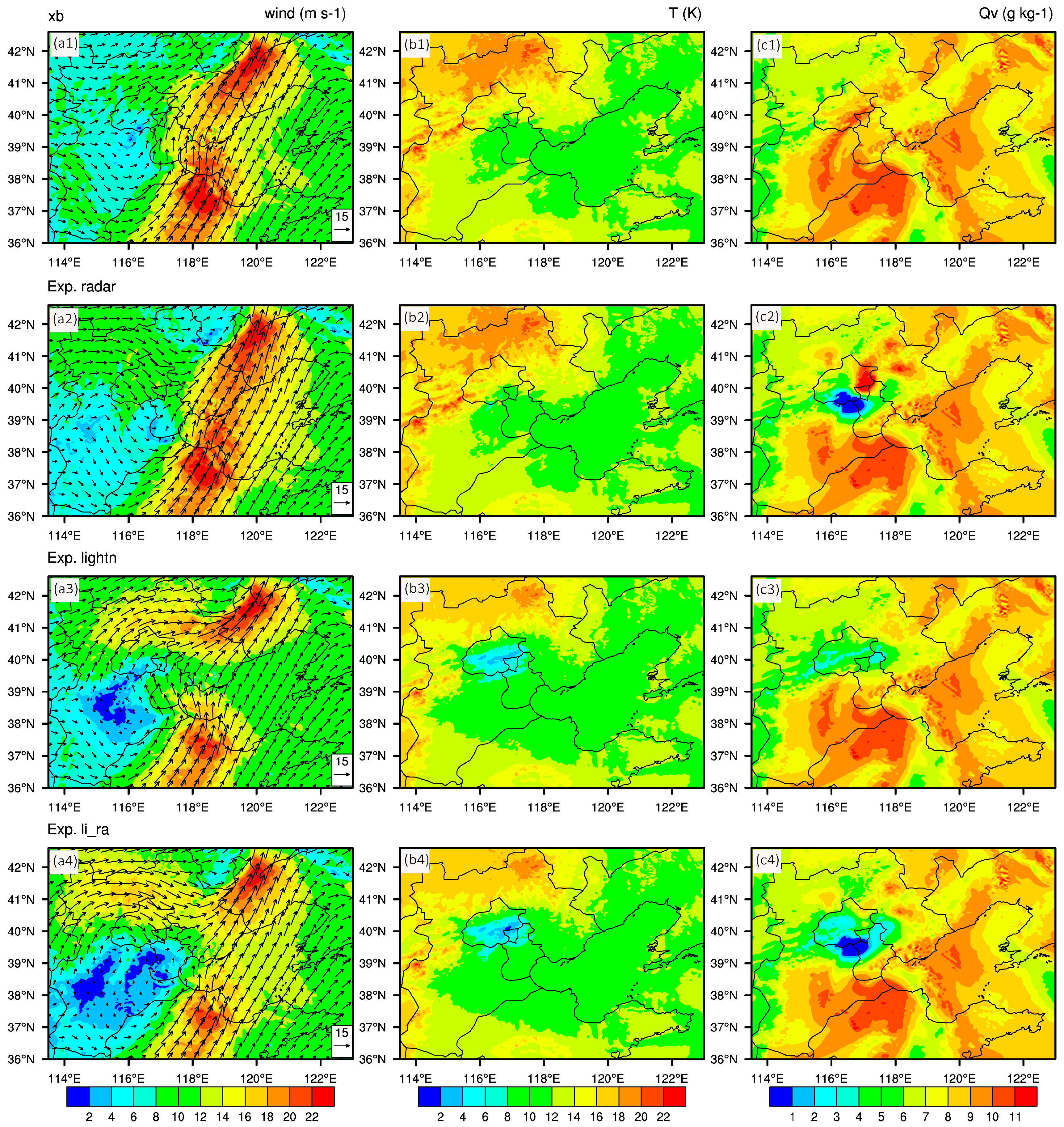
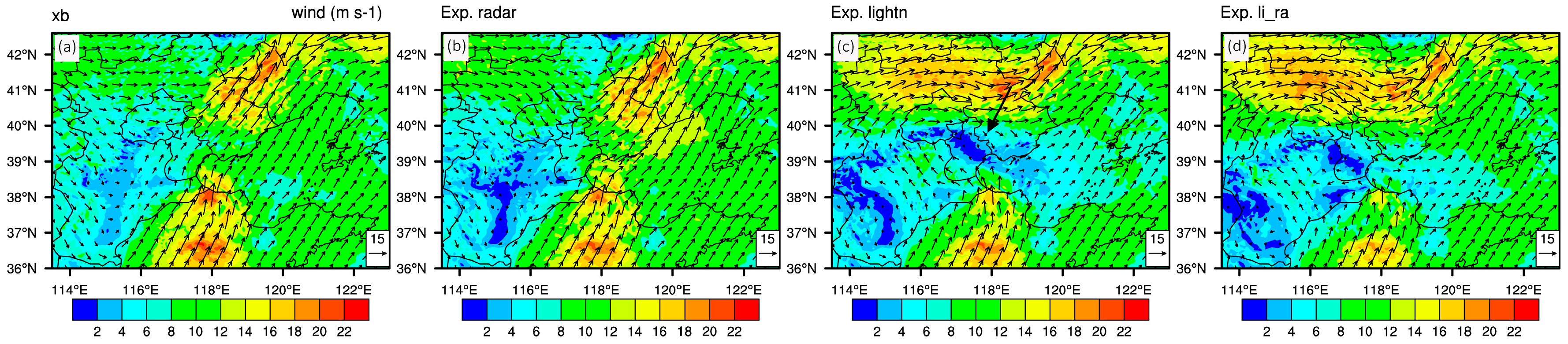
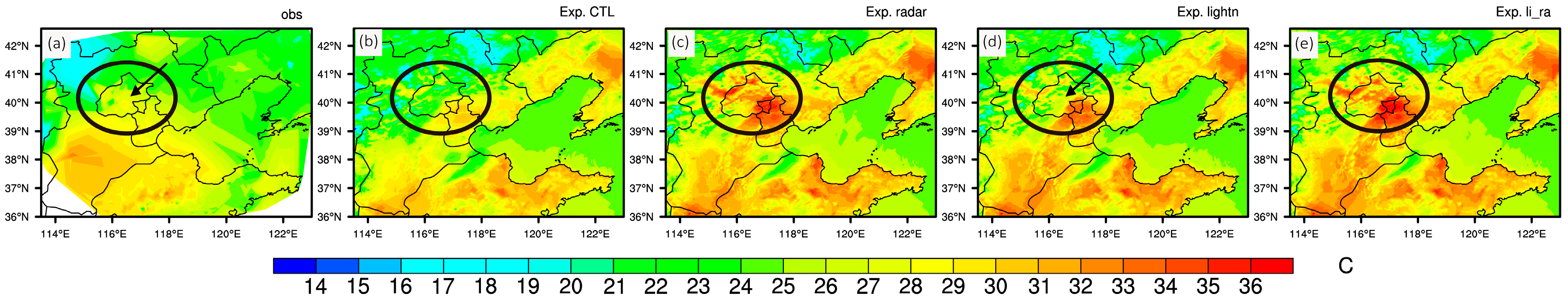
3.1. Analysis if the Terrain and Increments after Data Assimilation

The horizontal scope of the two nested domains, and model terrain height, are illustrated in Figure 1. Beijing is mainly surrounded by mountains to the west, north and east, including Yanshan Mountain to the north and Taihang Mountain to the west (Figure 1). In the second domain, terrain height decreases significantly from northwest to southeast. In events that affect Beijing and Tianjin, the squall line is mainly concentrated to the northwest of Yanshan Mountain and Taihang Mountain [53]. The terrain around Beijing is a forcing mechanism for squall line development. In northwesterly flow conditions, a strong cold air intrusion in the upper layer, and a strong frontogenesis forced by terrain in the lower layer may offer an excellent dynamic condition for squall line emergence and development. Thus, Beijing and Tianjin are often the locus of significant mesoscale convective systems in summer. In the squall line case on 31 July 2007, the first lightning was detected by SAFIR 3000 at 0300 UTC, with lightning flashes mainly located in Hebei Province, to the northwest of Beijing, which is the region where squall lines typically occur. With southward-moving cold air behind the cold front of a vortex over Northeast China, diabatic heating forced by the terrain convergence zone superposition process in the surface layer had a significant effect on squall line. In the following three hours, the region of severe convection on the squall line, as indicated by the observed lightning belt, extended from northeast to southwest, and moved southeastward. The squall line then affected Tianjin, south of Hebei Province, the Bohai Sea and the northern part of Shandong Provincein turn.
Figure 2 shows the assimilated observation data at 0300 UTC. The assimilated total lightning is mainly located in Beijing, oriented in a northeast to southwest direction. The assimilated radar reflectivity covers Beijing, north Tianjin and northern Hebei Province, with maximum reflectivity of 45 dBZ in northeast Hebei Province. Radar radial velocity at 1.5° elevation ranges between 10 m·s−1 and −18 m·s−1, with the maximum located in western and northeastern Hebei Province. In Figure 3, the horizontal background and analyzed fields of wind, perturbation potential temperature and water vapor mixing ratio at 0300 UTC are illustrated for the second domain (at level = 14, about 4 km). In the background field, a two-centered low level jet with northward airflow ranging from the north of Shandong Province to the west of Liaoning Province has wind speeds of more than 22 m·s−1, with cyclonic circulation to the west of the southern jet center. In Exp. radar, after assimilating radar reflectivity and radial velocity at 0300 UTC, the two jet centers are combined, the cyclonic circulation in southern Hebei Province is decreased and the wind direction over Beijing changes from southwesterly to northwesterly. In Exp. lightn, the two jet centers are separated and cover a slightly smaller area. The northern jet increases the northward airflow over Beijing and the southern jet increases peripheral airflow associated with the cyclonic circulation. In Exp. li_ra, the analyzed wind field is a combination of Exp. radar and Exp. lightn results. Airflow over Beijing is northwesterly, which can force the squall line to move downstream along the mountain front. The southern cyclonic circulation decreases significantly, with a minimum wind speed of less than 2 m·s−1.To clearly show the structure of low level jet over a layer, lower level (at level = 8, about 1.5 km) wind fields are shown in Figure 4. As with the higher level winds in Figure 3, Exp. lightn provides two jet centers, a northern one with westerly airflow and a southern one with southerly airflow. There is a wind convergence in southern Beijing and northern Tianjin (indicated by the black arrow in Figure 4c), which is the downstream area of severe convection (indicated by the location of observed lightning data at 0300 UTC in Figure 2a). Lower level wind convergence together with the higher level jet could increase vertical motion and stimulate the release of convective available potential energy, which provides effective dynamic conditions for the early development of a squall line. In the perturbation potential temperature field in Figure 3, Exp. lightn and Exp. li_ra provide a more pronounced decrease in Beijing, which indicates that assimilating lighting data can better reconstruct the cold pool structure in the early stage of squall line development. To validate the surface temperature against the observation, Figure 5 presents the horizontal surface temperature field for each experiments with the observed automatic weather station surface temperature field for validation. At the early stage of the squall line, a cold pool structure has not formed at surface. In Beijing and neighboring region (black circle in Figure 5), Exp. lightn gives the best analyzed temperature field against the observation with the temperature around 28 °C. In Exp. CTL, the surface temperature is about 23 °C, 5 °C lower than observed, which may lead to a decrease in vertical motion by underestimating the surface heating. However, in Exp. radar and Exp. li_ra, surface heating is overestimated. In Exp. lightn, the appropriate surface heating associated with a higher level cold pool produces a positive effect on the vertical updraft and release of latent heat condensation at higher levels, and together with the effective dynamic condition mentioned above promotes the development of squall line. In terms of the water vapor mixing ratio field in Figure 3, Exp. radar produces a decrease in southern Beijing and an increase in northeastern Beijing. Compared with Exp. radar, Exp. lightn has a slight reduction over Beijing, and Exp. li_ra has a decrease over Beijing that is similar in size to that in Exp. radar. Overall, Exp. lightn and Exp. li_ra produce a cold pool environment, which contains a negative increment in temperature and water vapor over Beijing and surroundings. As the squall line airstream moves along Yanshan Mountain, a terrain-induced-downburst combined with a cold pool structure may contribute to squall line development. Additionally, the low level jet presents a strong vertical wind shear which can accelerate the release of convective available potential energy and abundant water vapor for heavy rainfall.

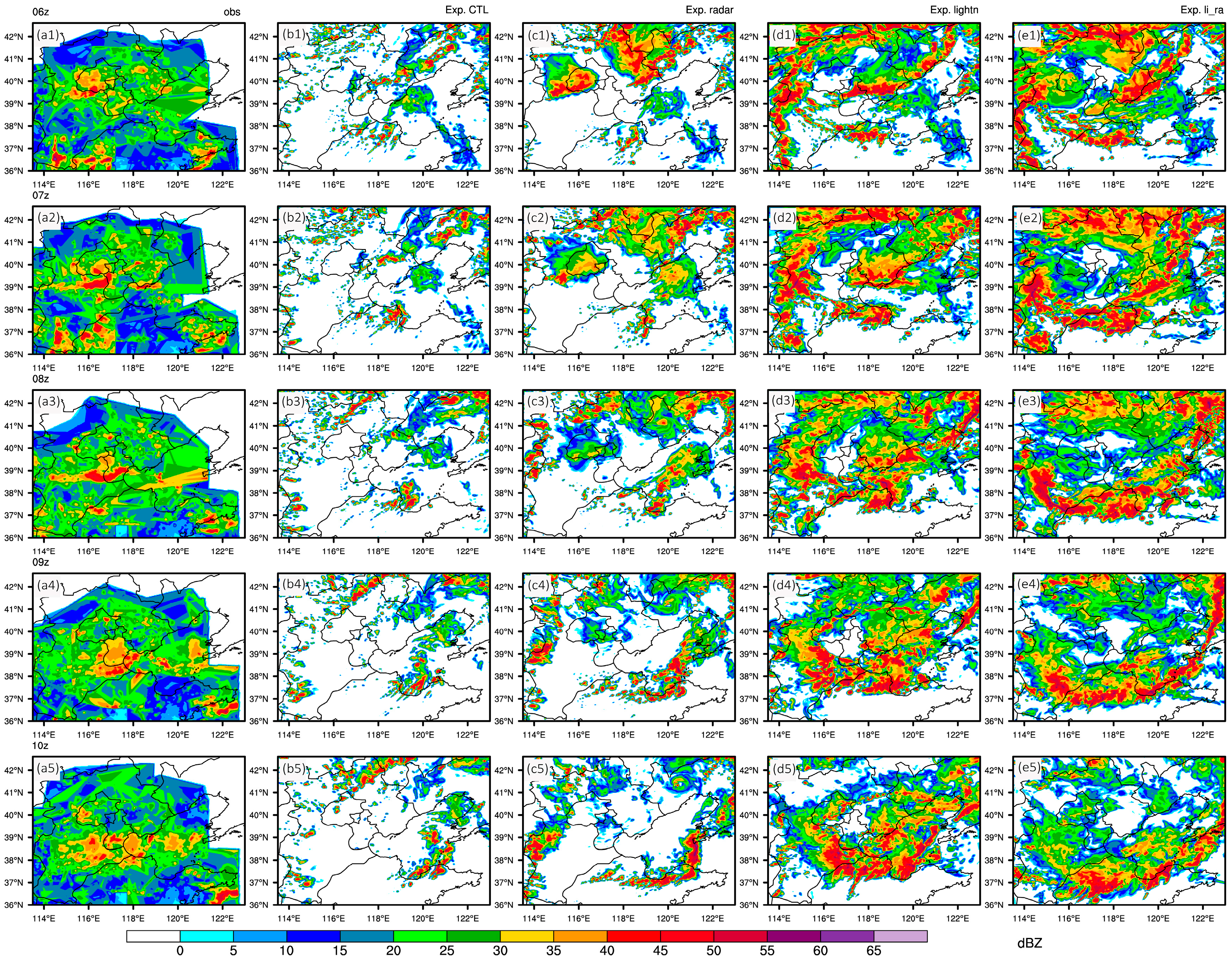
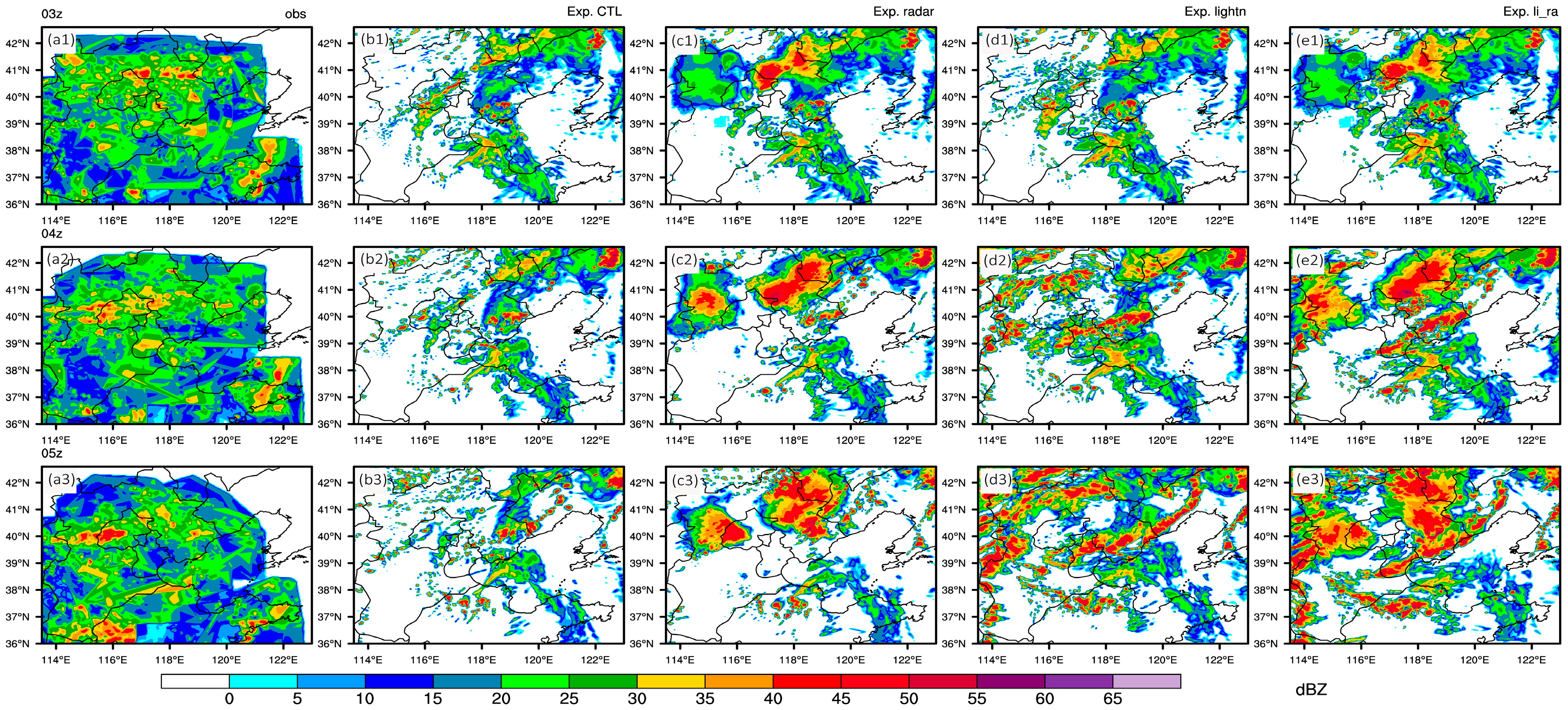
3.2. Analysis of the Forecast Maximum Reflectivity

Figure 6 shows 10 min forecast maximum reflectivity for the four experiments and radar observations in the second domain with 3 km resolution. The panel (a1–a3) shows observed radar reflectivity from six Doppler radars at Beijing, Tianjin, Shijiazhuang, Qinhuangdao, Jinan, and Qingdao. The panel (b–e) are maximum reflectivity forecasts from Exp. CTL, Exp. radar, Exp. lightn and Exp. li_ra in the sequential assimilation process. The squall line is in the early stage of development from 0300 to 0500 UTC. At 0500 UTC, the observed maximum squall line reflectivity is located west of Beijing. In Exp. CTL, there is limited evidence for the squall line. In Exp. radar, assimilating radar reflectivity and radial velocity gave better reconstruction of the high reflectivity belt in the west of Beijing and Hebei Province, however, the high reflectivity in northeast Hebei Province is overestimated. Combining the analysis in Figure 3, Figure 4 and Figure 5, the low level jet in Exp. radar transfers water vapor to the northeast of Hebei Province. Additionally, the overestimated surface heating in Exp. radar excessively increases the vertical motion. All these conditions lead to an overestimation of maximum radar reflectivity in northeastern of Hebei Province in Exp. radar. In Exp. lightn, the maximum reflectivity belt is mostly split into two parts, northern and southern. At 0500 UTC, the high reflectivity belt in Beijing is spatially displaced to the west, compared with observations, and the reflectivity belts in Tianjin and Liaoning Province are combined. Exp. li_ra provides a synthesis of Exp. radar and Exp. lightn results, reconstructing the belt in Beijing, but with spurious severe convection in Tianjin and western Liaoning Province.
Figure 7 shows the forecast maximum reflectivity of the four experiments and radar observations. In the observation, the squall line develops gradually and reaches its most extended state at 0800 UTC, in the form of an arch shape with maximum reflectivity above 45 dBZ. For Exp. CTL, the high reflectivity belt is poorly represented and is switched from Beijing to Tianjin for the entire period from 0600 to 1000 UTC. In Exp. radar, the reflectivity and radar radial velocity of the Beijing Doppler radar were assimilated at 0300, 0400 and 0500 UTC. At 0600 UTC, Exp. radar captures the main reflectivity in west to central part of Beijing and the high reflectivity belt in the southern part of Beijing is especially well represented, located in the same place as the observations and at similar strength, above 45 dBZ. By 0700 UTC, reflectivity decreases and moves slower than the observation, which leads to an underestimate in Tianjin. In all, the improvement given by assimilating radar reflectivity and radial velocity is only maintained for the first four hours and the affected area is limited. In the first three hours, maximum reflectivity in Exp. lightn is mostly located in the east and there is an obvious overestimation. Overestimation of maximum reflectivity around the boundary is most evident in the first few hours and disappears in later hours. This feature maybe due to the choice of the radius of influence. Lightning data are converted into relative humidity which is treated as sounding data in this study. Thus, the choice of the radius of influence is based on that of the sounding data, which is determined by the calculated background error covariances. In future work, treating proxy relative humidity as normal sounding data or observed data only utilized at the mesoscale needs to be explored further. At 0600 UTC, the high reflectivity belt in Exp. lightn is located further to the east and south compared with observations, and is higher in magnitude. At 0700 UTC, the belt in the eastern part of Tianjin and at the border of the Bohai Sea and Hebei Province is similar to observations. However, evidence for the main squall line in western Tianjin is still missing. In the last two hours, the southern belt in Tianjin and northern Shandong Province is close to observations, although still overestimated. At 1000 UTC, the reflectivity in Beijing and the southern part of Hebei Province is reconstructed well, which indicates that Exp. lightn provides a better forecast in the later hours than Exp. radar. Exp. li_ra can combine the advantages of Exp. radar and Exp. lightn, which better simulates the reflectivity in Beijing in the first two hours. Nevertheless, the main part of the squall line moves more quickly than the observation and is located further to the south. In the last two hours, the southern overestimation of Exp. lightn is corrected in Exp. li_ra, although the belt in southern Tianjin and west of the Bohai Sea is underestimated. In general, after sequential assimilation of lightning data, there is an obvious qualitative improvement in maximum reflectivity, and the improvement persists for more than five hours due to the excellent dynamic coordination between variables achieved using WRF-3DVAR. In particular, the superiority of Exp. lightn is shown in the last two hours so that both the southern reflectivity belt and the reflectivity in Beijing are well placed. Nevertheless, there is obvious overestimation in the southern part, which may indicate Exp. lightn over adjusts in such regions so that more severe convection is produced than actually observed.
Figure 7. Forecast composite maximum reflectivity (dBZ) of the four experiments from 0600 UTC to 1000 UTC. Panels (a1a5) show observed maximum reflectivity; and panel (be) show the maximum reflectivity of Exp. CTL, Exp. radar, Exp. lightn and Exp. li_ra at each of these 5 h, respectively (unit: dBZ).
Atmosphere 08 00055 g007

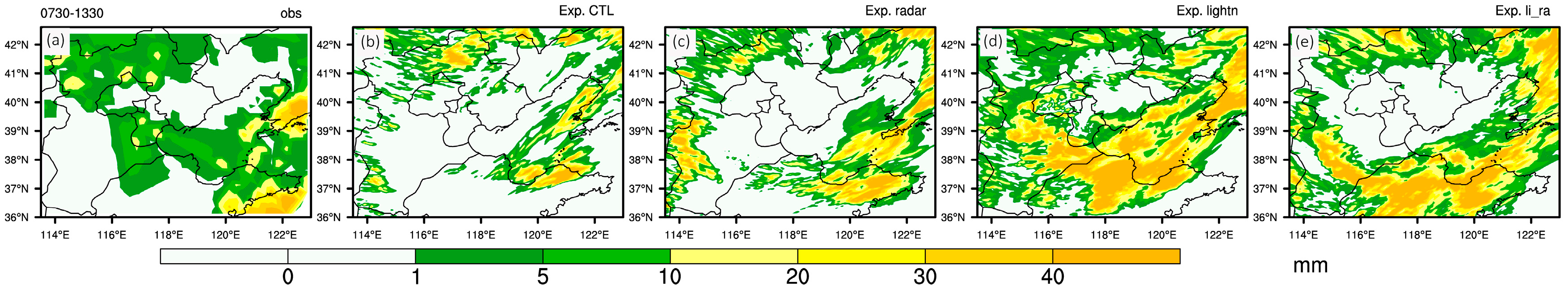
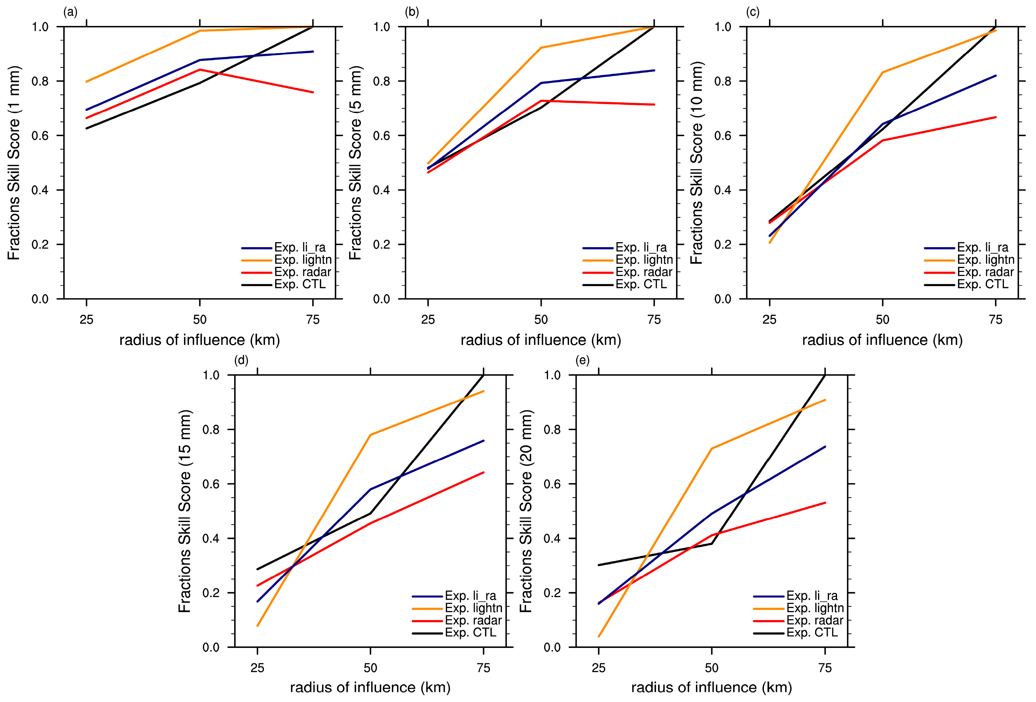
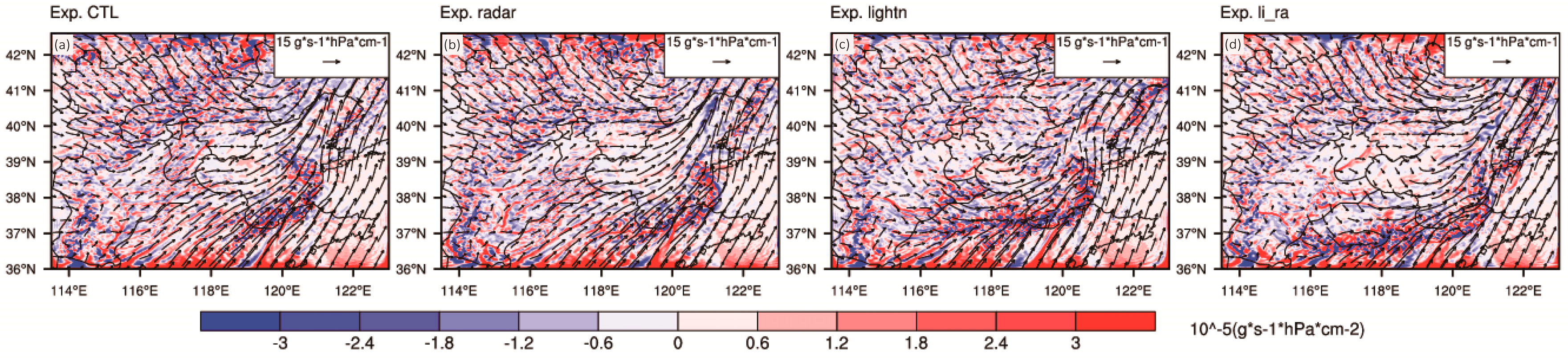
3.3. Analysis of the Forecast Precipitation

In convective weather, another important variable is precipitation. Figure 8 shows the forecast 6 h accumulated precipitation for the four experiments against the observations. The time interval of observation and forecast is 0730 to 1330 UTC. The observed precipitation is a combination of TRMM 3B42 observation data and automatic weather station data. The automatic weather station precipitation data are interpolated into the TRMM grid and then combined with the TRMM precipitation data with appropriate weighting. From 0730 to 1330 UTC, observed heavy precipitation centers (>20 mm) are mainly located in the northern and western part of Beijing, part of Tianjin, the Bohai Sea, southern Liaoning Province and southern Shandong Province. In particular, the maximum accumulated precipitation in Liaoning and Shandong Province is greater than 40 mm in 6 h. In Exp. CTL, the heavy center in Beijing is displaced to the north. The center in Liaoning Province is not forecast and the rainbelt in the northern part of Shandong Province is overestimated. Exp. radar provides a similar forecast as Exp. CTL. The overestimate for the center in northern Hebei Province is revised. There are also slight improvements in the Bohai Sea and the northern part of Shandong Province, so that precipitation quantity is closer to the observations. The Exp. lightn forecast is better than that in the previous two experiments. In northern and southern Hebei Province, Beijing, south Tianjin and southern Liaoning Province, the forecast accumulated precipitation is almost same as the observed. However, in most of the Bohai Sea and northern Shandong Province, accumulated precipitation is overestimated due to producing too much spurious severe convection (shown in Figure 7). In Exp. li_ra, the northern rain belt in Hebei Province is located well while the heavy center in Liaoning Province is more northerly. Additionally, the overestimated belt in northern Shandong Province is still forecast and this belt presents a more southern place than in Exp. lightn. Thus, in a qualitative analysis of 6 h accumulated precipitation, Exp. lightn provides a best forecast in the Beijing neighborhood of the four experiments. However, due to producing too many spurious severe convections, there are many overestimated rain belts in the rest of the domain. Considering the whole forecast in the domain, the improvement of precipitation forecast in Exp. lightn is not so obvious. To analyze the characteristics of 6 h accumulated precipitation in the experiments, water vapor flux and water vapor flux divergence at 850 hPa are illustrated in Figure 9. Water vapor flux indicates the transportation of water vapor that is needed in precipitation. The blue colored regions represent strong ascending convergence. Water vapor flux is abundant from Shandong Province to southern Liaoning Province in all four experiments. However, water vapor divergence shows different trends. In Exp. CTL, the region of ascending convergence is mainly located in northeastern Shandong Province. In Exp. radar, ascending convergence spreads inland, covering northern Shandong Province. When assimilating lightning data is included, the area and strength of ascending convergence is larger than in Exp. CTL and Exp. radar, covering southern Liaoning Province, northern Shandong Province and southeastern Hebei Province. In Exp. li_ra, the ascending convergence is located further south. In all, the water vapor flux and water vapor flux divergence explains the distinct location and strength of 6 h accumulated precipitation well.
A quantitative analysis of 6h accumulated forecast precipitation is given in Table 1. Threat scores (TS), false alarm ratio (FAR) and probability of detection(POD) are utilized to analyze the results at thresholds of 1 mm, 5 mm, 10 mm, 15 mm, and 20 mm. TS give a comprehensive skill score considering both the strength and location of precipitation. The FAR is the fraction of event forecasts associated with non-occurrences. The FAR can be controlled by deliberately under forecasting an event, but such a strategy risks increasing the number of missed events. POD is the ratio of detected aims to the number of all possible targets. Therefore, POD and FAR should both be considered for a better understanding of forecast performance. The perfect score for TS and POD is 1.00 and the no skill score is 0.00. The perfect score for FAR is 0.00 and the no skill score is 1.00. In terms of threat scores, the improvements of the assimilation experiments are not so obvious against the base control experiment. At a threshold of 1 mm, which indicates the precipitation region, the TS of Exp. li_ra slightly improves with the value of 0.50,while that of Exp. CTL is only 0.44. At thresholds of 5 mm, 10 mm, 15 mm and 20 mm, Exp. radar obtains the optimal values. For the FAR, Exp. radar performs best at thresholds of 10 mm, 15 mm and 20 mm. At high thresholds, all four experiments have high FARs especially for the threshold of 20 mm, which is verified by too much spurious severe convection in Figure 7. For POD, the highest results are for Exp. li_ra, with values of0.81, 0.61, and 0.41 at thresholds of 1 mm, 5 mm, and 10 mm, respectively. At thresholds of 15 mm and 20 mm, Exp. lightn obtains the highest values. The TS, FAR and POD do not take spatial displacement into account. To give a more effective evaluation of the location of 6 h accumulated precipitation, a neighborhood spatial verification method, the fractions skill score (FSS) [54] is utilized (shown in Figure 10). The FSS ranges from 0.00 to 1.00 with a perfect value of 1.00. The radius of influence varies from 25 km to 75 km. At the 1 mm threshold, the FFS value for Exp. lightn is 0.80 at 25 km, and it maintains this superiority as the radius of influence increases to 50 km and 75 km. At higher thresholds, the different between these three assimilation experiments is more obvious. At all thresholds, Exp. lightn gives the best result at the radius of 50 km, which indicates that the location of forecast precipitation can be improved through assimilating lightning data. Therefore, in a comprehensive analysis of 6 h accumulated precipitation including horizontal distribution, TS, FAR, POD and FSS, a quantitative improvement cannot be achieved in these three assimilation experiments due to producing too much false precipitation in the analyzed domain. However, in the spatial distribution of the forecast rain belt, Exp. lightn presents the optimal result, though magnitude of the southern6 h accumulated precipitation is strongly overestimated.

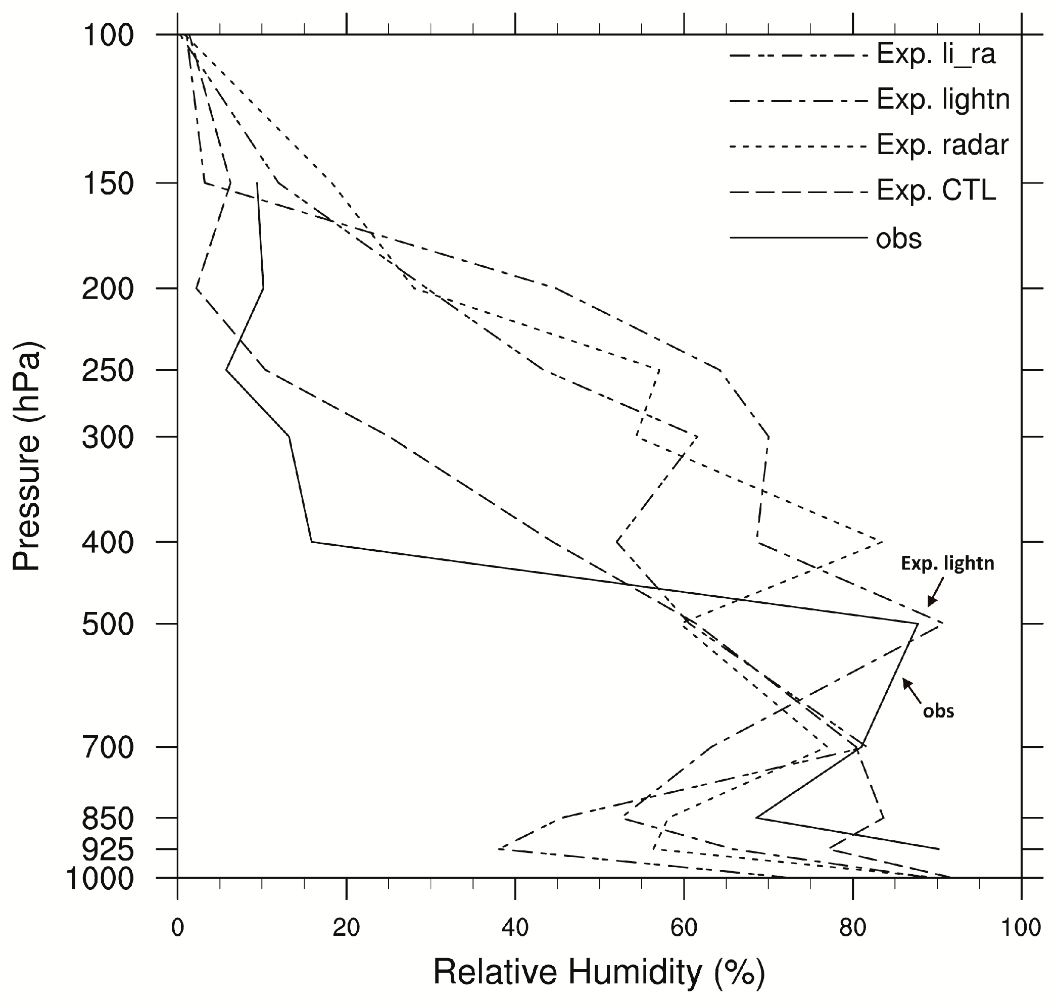
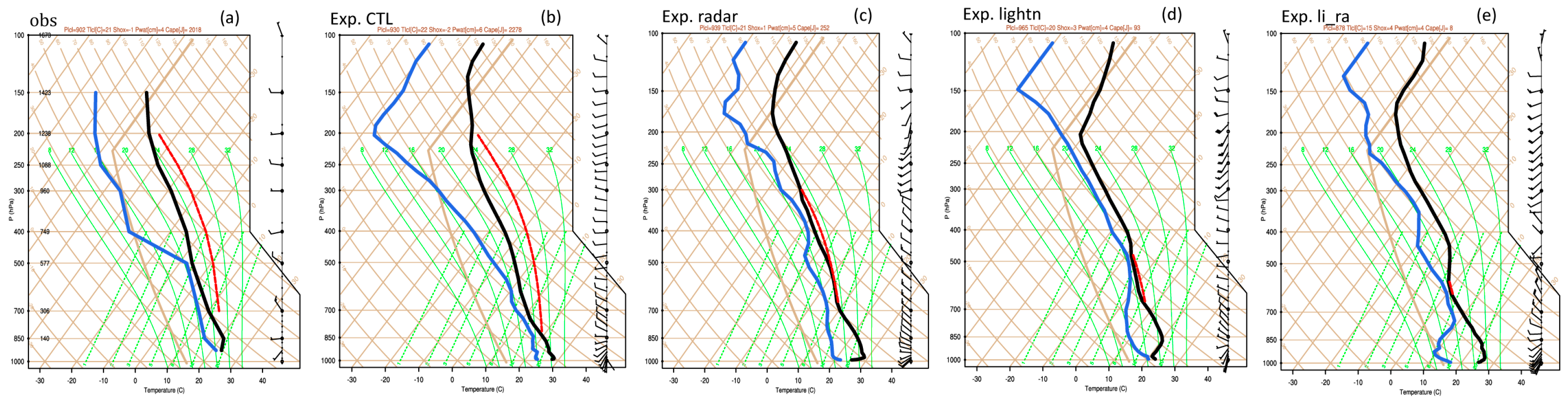
3.4. Analysis of the Stratification Curve

The above discussion elaborates the forecast improvement using Exp. lightn. Compared with radar data assimilation, the improvements of lightning data assimilation may be delayed by a few hours. To analyze the vertical improvement of the stratification curve in the later hours, skew-T diagrams for observations, Exp. CTL, Exp. radar, Exp. lightn and Exp. li_ra at Beijing, 1200 UTC, are illustrated in Figure 11. Among all these four experiments, Exp. lightn provides the best profile compared with the observed. There is a temperature inversion layer below 850 hPa in the observed profile, which is captured in the Exp. lightn profile but not in that of Exp. CTL. Similarly, the shape of the dew-point temperature and temperature profiles for Exp. lightn match the observation. From 700 hPa to 500 hPa, the temperature profile is close to that of the dew-point temperature, with an inverse bell shape. From 700 hPa to 500 hPa humidity condition is pretty similar as the observed one (the shape of the temperature profile and dew-point temperature profile are similar), which offers a proper humidity condition in this layer. For validation, the relative humidity profiles of these four experiments are compared with that of observations at Beijing illustrated in Figure 12. From 925 hPa to 500 hPa, the trend of relative humidity profile in Exp. lightn is similar to observed relative humidity profile. In particular, Exp. lightn provides the best humidity condition from 700 hPa to 500 hPa against the observation at 1200 UTC at Beijing7 h after the assimilation time. For the layer above 300 hPa, the relative humidity profile in Exp. CTL is similar to the observed. However, Exp. lightn has some limitations. In Figure 11, the convective available potential energy in the observation is about 2018 J while that in Exp. lightn is only 93 J and is restricted to the layer from 700 hPa to 500 hPa. This Exp. lightn stratification curve means that convective activity after 1200 UTC is restricted to the layer, which does not match well with the observation. Overall, based on sequential lightning data assimilation, Exp. lightn gives an obvious improvement in the stratification curve below 500 hPa and the correct humidity condition from 700 hPa to 500 hPa even 7 h after the assimilation time.

4. Conclusions

Lightning network data, as a new source of observational data in convective systems, can remedy the temporal and spatial disadvantages of radar data. Furthermore, lightning can indicate the occurrence and development of mesoscale convective systems due to its strong relationship with dynamic and microphysical processes. Thus, a method of lightning data assimilation that can reconstruct the relationship between lightning and other model variables is essential. The 3DVAR method benefits from dynamic coordination between variables based on background error covariance. Lightning data are first transformed into the water vapor mixing ratio using the relationship reported by Fierro et al. [27].The calculated water vapor mixing ratio is then converted into relative humidity as sounding data that can be utilized in WRFDA. This method mainly adjusts the mixed-phase region between the 0 °C and −20 °C isotherms, which is the electrification layer of ice and water and is strongly associated with convective activity. The benefits of assimilating lightning data by WRF-3DVAR are demonstrated in a series of experiments using data from a strong convection event that occurred in Beijing, China on 31 July 2007. The conclusions of this case study are summarized as follows.
(1)
Transforming total lightning data into proxy relative humidity is a simple and effective method, and assimilating lightning data with WRF-3DVAR can easily be implemented in many existing operational model platforms.
(2)
With sequential lightning data assimilation, forecast maximum reflectivity improves considerably and is sustained. Compared with assimilating radar reflectivity and radial velocity, assimilating lightning data can achieve a better improvement in the sustainment. In later hours, particularly in the assimilated lightning data region, the forecast maximum reflectivity in Exp. lightn is well reconstructed compared with the observations.
(3)
After assimilating lightning data, the 6 h accumulated precipitation forecast gains some improvements according to the fraction skill score at a spatial resolution of 50 km. The intensity of precipitation around assimilated lightning and neighboring areas is closer to the observations, although some regional precipitation is overestimated. The precipitation forecast in the downstream area is also considerably improved (e.g., both the position and intensity of the heavy rainfall center in Liaoning Province is corrected). However, a significant improvement cannot be achieved in Exp. lightn due to producing excessive false precipitation in the southern area. Thus, a future direction for lightning data assimilation research might be how to best use observations or methods to suppress spurious severe convection.
(4)
Basing on sequential lightning data assimilation, Exp. lightn gives an obvious improvement in the stratification curve below 500 hPa at 7 h after the assimilation. Although the calculated convective available potential energy is smaller than the observation, the temperature and dew-point temperature profile match the observed, perfectly reconstructing humidity conditions from 700 hPa to 500 hPa.
In this case study, lightning data assimilation has performed well and there is good potential to implement it in many existing operational model platforms. Nevertheless, the spurious severe convection produced in lightning data assimilation needs to be studied further. In the case study, the choice of influence radius in the 3DVAR framework is based on the influence radius of sounding data, which is determined by the calculated background error covariances. In future work, treating proxy relative humidity as normal sounding data or mesoscale data needs to be explored further. We would also like to test more cases to examine the utility of the method and to derive our own relationship between flash data and other variables based on the China lightning network data to find a more dynamically consistent method of assimilating lightning data, to better reconstruct the flow field in mesoscale systems and provide a sounder physical basis to lightning data assimilation.

Acknowledgments

This research was supported by the National Key Basic Research Program of China (No. 2014CB441406) and the National Science Foundation of China (No. 41175092). The authors thank the Institute of Atmospheric and Physics, Information Center of China Meteorological Administration and Chinese Academy of Meteorological Sciences for providing lightning and precipitation data. The lightning and Doppler radar data can be obtained by data application to the Data Center of Chinese Meteorological Administration (http://data.cma.cn/).

Author Contributions

Yi Yang provided the initial idea of this paper. Ying Wang designed, performed the experiment and wrote the paper under the guidance of Yi Yang. Dongxia Liu, Dongbin Zhang and Wen Yao provided the observation data and promoted useful suggestions on data processing. Chenghai Wang provided some useful advice in the analysis and discussion part.

Conflicts of Interest

The authors declare no conflict of interest.

References

  1. Latham, J.; Petersen, W.A.; Deierling, W.; Christian, H.J. Field identification of a unique globally dominant mechanism of thunderstorm electrification. Q. J. R. Meteorol. Soc. 2007, 133, 1453–1457. [Google Scholar] [CrossRef]
  2. Reynolds, S.E.; Brook, M.; Gourley, M.F. Thunderstorm Charge Separation. J. Meteorol. 1957, 14, 426–436. [Google Scholar] [CrossRef]
  3. López, R.E.; Aubagnac, J.P. The lightning activity of a hailstorm as a function of changes in its microphysical characteristics inferred from polarimetric radar observations. J. Geophys. Res. 1997, 102, 16799–16813. [Google Scholar] [CrossRef]
  4. Sabbas, F.T.S.; Sentman, D.D. Dynamical relationship of infrared cloudtop temperatures with occurrence rates of cloud-to-ground lightning and sprites. Geophys. Res. Lett. 2003, 30. [Google Scholar] [CrossRef]
  5. Williams, E.R.; Weber, M.E.; Orville, R.E. The relationship between lightning type and convective state of thunderclouds. J. Geophys. Res. 1989, 94, 13213–13220. [Google Scholar] [CrossRef]
  6. Zhang, T.; Zhao, Z.; Zhao, Y.; Wei, C.; Yu, H.; Zhou, F. Electrical soundings in the decay stage of a thunderstorm in the Pingliang region. Atmos. Res. 2015, 164–165, 188–193. [Google Scholar] [CrossRef]
  7. Michaelides, S.; Savvidou, K.; Nicolaides, K. Relationships between lightning and rainfall intensities during rainy events in Cyprus. Adv. Geosci. 2010, 23, 87–92. [Google Scholar] [CrossRef] [Green Version]
  8. Stolz, D.C.; Businger, S.; Terpstra, A. Refining the relationship between lightning and convective rainfall over the ocean. J. Geophys. Res. Atmos. 2014, 119, 964–981. [Google Scholar] [CrossRef]
  9. Tapia, A.; Smith, J.A.; Dixon, M. Estimation of convective rainfall from lightning observations. J. Appl. Meteorol. 1998, 37, 1497–1509. [Google Scholar] [CrossRef]
  10. Zhou, Y.; Qie, X.; Soula, S. A study of the relationship between cloud-to-ground lightning and precipitation in the convective weather system in China. Ann. Geophys. 2002, 20, 107–113. [Google Scholar] [CrossRef]
  11. Stefanescu, R.; Navon, I.M.; Fuelberg, H.; Marchand, M. 1D+4D-VAR data assimilation of lightningwith WRFDA system using nonlinear observation operators. arXiv, 2013; arXiv:1306.1884. [Google Scholar]
  12. Tinmaker, M.I.R.; Aslam, M.Y.; Chate, D.M. Lightning activity and its association with rainfall and convective available potential energy over Maharashtra. India Nat. Hazards 2015. [Google Scholar] [CrossRef]
  13. Price, C.; Rind, D. A simple lightning parameterization for calculating global lightning distributions. J. Geophys. Res. 1992, 97, 9919–9933. [Google Scholar] [CrossRef]
  14. Benjamin, S. Assimilation of lightning data into RUC model convection forecasting. In Proceedings of the Second Conference on Meteorological Applications of Lightning Data, Tucson, AZ, USA; 2006. Available online: https://ams.confex.com/ams/Annual2006/techprogram/paper_105079.htm (accessed on 31 January 2006). [Google Scholar]
  15. Benjamin, S.; Weygandt, S.; Brown, J.; Smirnova, T.; Devenyi, D.; Brundage, K.; Grell, G.; Peckham, S.; Schlatter, T.; Smith, T. From the radar-enhanced RUC to the WRF-based Rapid Refresh. In Proceedings of the 18th Conference on Numerical Weather Prediction, Park City, UT, USA, 25–29 June 2007.
  16. Benjamin, S.G.; Dévényi, D.; Weygandt, S.S.; Brundage, K.J.; Brown, J.M.; Grell, G.A.; Kim, D.; Schwartz, B.E.; Smirnova, T.G.; Smith, T.L. An hourly assimilation-forecast cycle: The RUC. Mon. Weather Rev. 2004, 132, 495–518. [Google Scholar] [CrossRef]
  17. Weygandt, S.S.; Benjamin, S.G.; Smirnova, T.G.; Brown, J.M. Assimilation of lightning data using a diabatic digital filter within the Rapid Update Cycle. In Proceedings of the 12th Conference on IOAS-AOLS, New Orleans, LA, USA, 20–24 Jaunary 2008.
  18. Bovalo, C.; Barthe, C.; Pinty, J.; Chong, M. Potential of cloud-resolving model parameters to be used as proxies for the total flash rate. In Proceedings of theXV International Conference on Atmospheric Electricity, Norman, OK, USA, 15–20 June 2014.
  19. Barthe, C.; Deierling, W.; Barth, M.C. Estimation of total lightning from various storm parameters: A cloud-resolving model study. J. Geophys. Res. 2010, 115, D24202. [Google Scholar] [CrossRef]
  20. Deierling, W.; Petersen, W.A.; Latham, J.; Ellis, S.; Christian, H.J. The relationship between lightning activity and ice fluxes in thunderstorms. J. Geophys. Res. 2008, 113, D15210. [Google Scholar] [CrossRef]
  21. Deierling, W.; Petersen, W.A. Total lightning activity as an indicator of updraft characteristics. J. Geophys. Res. 2008, 113, D16210. [Google Scholar] [CrossRef]
  22. Kuhlman, K.M.; Ziegler, C.L.; Mansell, E.R.; MacGorman, D.R.; Straka, J.M. Numerically simulated electrification and lightning of the 29 June 2000 STEPS supercell storm. Mon. Weather. Rev. 2006, 134, 2734–2757. [Google Scholar] [CrossRef]
  23. Alexander, G.D.; Weinman, J.A.; Karyampudi, V.M.; Olson, W.S.; Lee, A.C.L. The Effect of Assimilating Rain Rates Derived from Satellites and Lightning on Forecasts of the 1993 Superstorm. Mon. Weather Rev. 1999, 127, 1433–1457. [Google Scholar] [CrossRef]
  24. Chang, D.E.; Weinman, J.A.; Morales, C.A.; Olson, W.S. The Effect of Spaceborne Microwave and Ground-Based Continuous Lightning Measurements on Forecasts of the 1998 Groundhog Day Storm. Mon. Weather Rev. 2001, 129, 1809–1833. [Google Scholar] [CrossRef]
  25. Papadopoulos, A.; Chronis, T.G.; Anagnostou, E.N. Improving convective precipitation forecasting through assimilation of regional lightning measurements in a mesoscale model. Mon. Weather. Rev. 2005, 133, 1961–1977. [Google Scholar] [CrossRef]
  26. Qie, X.; Zhu, R.; Yuan, T.; Wu, X.; Li, W.; Liu, D. Application of total-lightning data assimilation in a mesoscale convective system based on the WRF model. Atmos. Res. 2014, 145–146, 255–266. [Google Scholar] [CrossRef]
  27. Fierro, A.O.; Mansell, E.R.; Ziegler, C.L.; MacGorman, D.R. Application of a Lightning Data Assimilation Technique in the WRF-ARW Model at Cloud-Resolving Scales for the Tornado Outbreak of 24 May 2011. Mon. Weather Rev. 2012, 140, 2609–2627. [Google Scholar] [CrossRef]
  28. Gallus, W.A., Jr.; Segal, M. Impact of improved initialization of mesoscale features on convective system rainfall in 10-km Eta simulations. Weather Forecast. 2001, 16, 680–696. [Google Scholar] [CrossRef]
  29. Mansell, E.R.; Ziegler, C.L.; MacGorman, D.R. A Lightning Data Assimilation Technique for Mesoscale Forecast Models. Mon. Weather Rev. 2007, 135, 1732–1748. [Google Scholar] [CrossRef]
  30. Lagouvardos, K.; Kotroni, V.; Defer, E.; Bousquet, O. Study of a heavy precipitation event over southern France, in the frame of HYMEX project: Observational analysis and model results using assimilation of lightning. Atmos. Res. 2013, 134, 45–55. [Google Scholar] [CrossRef]
  31. Mansell, E.R. Storm-Scale Ensemble Kalman Filter Assimilation of Total Lightning Flash-Extent Data. Mon. Weather Rev. 2014, 142, 3683–3695. [Google Scholar] [CrossRef]
  32. Wang, Y.; Yang, Y.; Wang, C. Improving forecasting of strong convection by assimilating cloud-to-ground lightning data using the physical initialization method. Atmos. Res. 2014, 150, 31–41. [Google Scholar] [CrossRef]
  33. Yang, Y.; Wang, Y.; Zhu, K. Assimilation of Chinese Doppler Radar and Lightning Data Using WRF-GSI: A Case Study of Mesoscale Convective System. Adv. Meteorol. 2015. [Google Scholar] [CrossRef]
  34. Yang, Y.; Qiu, C.; Gong, J. Physical initialization applied in WRF-Var for assimilation of Doppler radar data. Geophys. Res. Lett. 2006, 33. [Google Scholar] [CrossRef]
  35. Marchand, M.R.; Fuelberg, H.E. Assimilation of Lightning Data Using a Nudging Method Involving Low-Level Warming. Mon. Weather Rev. 2014, 142, 4850–4871. [Google Scholar] [CrossRef]
  36. Fierro, A.O.; Gao, J.; Ziegler, C.L.; Mansell, E.R.; MacGorman, D.R. Evaluation of a Cloud-Scale Lightning Data Assimilation Technique and a 3DVAR Method for the Analysis and Short-Term Forecast of the 29 June 2012 Derecho Event. Mon. Weather Rev. 2014, 142, 183–202. [Google Scholar] [CrossRef]
  37. Fierro, A.O.; Clark, A.J.; Mansell, E.R.; Macgoraman, D.R.; Dembek, S.R.; Ziegler, C.L. Impact of Storm-Scale Lightning Data Assimilation on WRF-ARW Precipitation Forecasts during the 2013 Warm Season over the Contiguous United States. Mon. Weather Rev. 2015, 143, 757–777. [Google Scholar] [CrossRef]
  38. Zou, X.; Navon, I.M.; LeDimet, F.X. An Optimal Nudging Data Assimilation Scheme Using Parameter Estimation. Q. J. R. Meteorol. Soc. 1992, 118, 1163–1186. [Google Scholar] [CrossRef]
  39. Sun, J. Convective-scale assimilation of radar data: Progress and challenges. Q. J. R. Meteorol. Soc. 2005, 131, 3439–3463. [Google Scholar] [CrossRef]
  40. Sun, J.; Xue, M.; Wilson, J.; Zawadzki, I.; Ballard, S.; Onvlee-Hooimeyer, J.; Joe, P.; Barker, D.; Li, P.; Golding, B.; et al. Use of NWP for Nowcasting Convective Precipitation: Recent Progress and Challenges. Bull. Am. Meteorol. Soc. 2014, 95, 409–426. [Google Scholar] [CrossRef]
  41. Parrish, D.F.; Derber, J.C. The National Meteorological Center’s Statistical SpectralInterpolation Analysis System. Mon. Weather Rev. 1992, 109, 1747–1763. [Google Scholar] [CrossRef]
  42. Xiao, Q.; Guo, Y.H.; Sun, J.; Lee, W.C.; Barker, D.M.; Lim, E. An Approach of Radar Reflectivity Data Assimilation and Its Assessment with the Inland QPF of Typhoon Rusa (2002) at Landfall. J. Appl. Meteorol. Clim. 2007, 46, 14–22. [Google Scholar] [CrossRef]
  43. Sun, J.; Crook, N.A. Dynamical and Microphysical Retrieval from Doppler Radar Observations Using a Cloud Model and Its Adjoint. Part I: Model Development and Simulated Data Experiments. J. Atmos. Sci. 1997, 54, 1642–1661. [Google Scholar] [CrossRef]
  44. Meng, Q.; Ge, R.S.; Zhu, X.Y. SAFIR lightning monitoring and alerting system. Meteorol. Sci. Technol. 2002, 30, 135–138. [Google Scholar]
  45. Li, X.J. Analysis of Lightning Characteristics Based on SAFIR Data in Beijing and Its Circumjacent Regions. Master’s Thesis, Nanjing University of Information Science and Technology, Nanjing, China, June 2011. [Google Scholar]
  46. Hong, S.-Y.; Lim, J.-O.J. The WRF Single-Moment 6-Class Microphysics Scheme (WSM6). J. Korean Meteorol. Soc. 2006, 42, 129–151. [Google Scholar]
  47. Mlawer, E.J.; Taubman, S.J.; Brown, P.D.; Iacono, M.J.; Clough, S.A. Radiative transfer for inhomogeneous atmospheres: RRTM, a validated correlated-k model for the longwave. J. Geophys. Res. Atmos. 1997, 102, 16663–16682. [Google Scholar] [CrossRef]
  48. Chou, M.-D.; Suarez, M.J. A solar radiation parameterization for atmospheric studies. NASA Tech. Memo 1999, 104606, 40. [Google Scholar]
  49. Smirnova, T.G.; Brown, J.M.; Benjamin, S.G. Performance of different soil model configurations in simulating ground surface temperature and surface fluxes. Mon. Weather Rev. 1997, 125, 1870–1884. [Google Scholar] [CrossRef]
  50. Nakanishi, M. Improvement of the Mellor-Yamada turbulence closure model based on large-eddy simulation data. Bound. Layer Meteorol. 2001, 99, 349–378. [Google Scholar] [CrossRef]
  51. Grell, G.A. Prognostic Evaluation of Assumptions Used by Cumulus Parameterizations. Mon. Weather Rev. 1993, 121, 764–787. [Google Scholar] [CrossRef]
  52. Grell, G.A.; Dévényi, D. A generalized approach to parameterizing convection combining ensemble and data assimilation techniques. Geophys. Res. Lett. 2002, 29, 1693. [Google Scholar] [CrossRef]
  53. Li, H.; Cai, Z.; Xu, Y. A Numereical Experiment of Topographic Effect on Genesis of the Squall Line in North China. Chin. J. Atmos. Sci. 1999, 23, 714–721. [Google Scholar]
  54. Roberts, N.M.; Lean, H.W. Scale-selective verification of rainfall accumulations from high-resolution forecasts of convective events. Mon. Weather Rev. 2008, 136, 78–97. [Google Scholar] [CrossRef]
Figure 1. Horizontal extent of the two nested domains and model terrain height distribution (unit: m). The resolutions of these two domains are 9 km and 3 km. Major Provinces and mountains are labeled and locations of three SAFIR (Surveillance et Alerte Foudre par Interferometrie Radiometrique) 3000 observation sites are marked with white dots.
Atmosphere 08 00055 g001
Figure 2. Assimilated observation data at 0300 UTC (Universal Time Coordinated) showing (a) location of observed total lightning from 0250 to 0300 UTC; (b) radar reflectivity at 1.5° elevation; and (c) radar radial velocity at 1.5° elevation. The Beijing Doppler radar location is marked with a black dot in (b,c). Five other Doppler radar locations are marked with red dots in (c).
Atmosphere 08 00055 g002
Figure 3. Background (xb) and analyzed (Exp. radar, Exp. lightn and Exp. li_ra) fields for (a) wind (m·s−1); (b) perturbation potential temperature (K); and (c) water vapor mixing ratio (g·kg−1) (at level = 14, about 4 km) at 0300 UTC.
Atmosphere 08 00055 g003
Figure 4. Background (xb) (a); and analyzed fields for (b) Exp. Radar;(c) Exp. Lightn; and (d) Exp. li_ra for wind (m·s−1) (at level = 8, about 1.5 km) at 0300 UTC.
Atmosphere 08 00055 g004
Figure 5. Observed surface temperature (a); and the surface temperature filed in Exp. CTL (b); Exp. radar (c); Exp. lightn (d); and Exp. li_ra (e) at 0300 UTC(unit: °C).
Atmosphere 08 00055 g005
Figure 6. Ten minute forecast maximum reflectivity (dBZ) of the four experiments from 0300 UTC to 0500 UTC. Panels (a1a3) show observed maximum reflectivity from the six Doppler radars at Beijing, Tianjin, Shijiazhuang, Qinghuangdao, Jinan and Qingdao, and panels (be) show the maximum reflectivity of Exp. CTL, Exp. radar, Exp. lightn and Exp. li_raat each of these 3 h, respectively (unit: dBZ).
Atmosphere 08 00055 g006
Figure 8. Forecast 6 h accumulated precipitation for: (a) observation; (b) Exp. CTL; (c) Exp. Radar; (d) Exp. Lightn; and (e) Exp. li_ra (unit: mm).
Atmosphere 08 00055 g008
Figure 9. Water vapor flux (g·s−1·hPa·cm−1) andwater vapor flux divergence (g·s−1·hPa·cm−2) in: (a) Exp. CTL; (b) Exp. Radar; (c) Exp. Lightn; and (d) Exp. li_ra at 850 hPa, 1030 UTC. The vector represents water vapor flux and the contour represents divergence of water vapor flux.
Atmosphere 08 00055 g009
Figure 10. Fractions Skill Score (FSS) for different thresholds of 6 h accumulated precipitation ((a) 1 mm; (b) 5 mm; (c) 10 mm; (d) 15 mm; and (e) 20 mm) in Exp. CTL, Exp. radar, Exp. lightn and Exp. li_ra. The perfect value of FSS is 1.00.
Atmosphere 08 00055 g010
Figure 11. Skew-T diagram for (a) observations; (b) Exp. CTL; (c) Exp. radar; (d) Exp. lightn; and (e) Exp. li_ra at Beijing, 1200 UTC. The blue line is the dew-point temperature profile and the black line is the temperature profile. The area between the black and red dashed lines indicates the convective available potential energy, which is calculated as 2018 J, 2278 J, 252 J, 93 J and 8 J for panels in (ae), respectively.
Atmosphere 08 00055 g011
Figure 12. Relative humidity profile forobservations, Exp. CTL, Exp. radar, Exp. lightn and Exp. li_ra at Beijing, 1200 UTC.
Atmosphere 08 00055 g012
Table 1. Threat scores (TS), false alarm ratio (FAR) and probability of detection (POD) for the 6 h accumulated precipitation in Exp. CTL, Exp. radar, Exp. lightn and Exp. li_ra at thresholds of 1 mm, 5 mm, 10 mm, 15 mm and 20 mm. Gray shaded areas denote the best results for each threshold level. The perfect score for TS and POD is 1.00 and the no skill score is 0.00. The perfect score for FAR is 0.00 and the no skill score is 1.00.
CategoryThresholdsExp. CTLExp.Radar RadarExp.LightnLilililightnExp.li_ra
TS1 mm0.44 0.47 0.47 0.50
5 mm0.21 0.260.22 0.23
10 mm0.07 0.150.09 0.12
15 mm0.02 0.090.04 0.05
20 mm0.01 0.080.04 0.03
FAR1 mm0.330.390.47 0.43
5 mm0.610.630.75 0.72
10 mm0.87 0.780.90 0.86
15 mm0.96 0.870.95 0.94
20 mm0.98 0.880.95 0.96
POD1 mm0.56 0.68 0.80 0.81
5 mm0.32 0.47 0.59 0.61
10 mm0.15 0.32 0.39 0.41
15 mm0.05 0.21 0.220.18
20 mm0.02 0.18 0.220.09

