
The Effect of Meteorological Elements on Continuing Heavy Air Pollution: A Case Study in the Chengdu Area during the 2014 Spring Festival

Plateau Atmosphere and Environment Key Laboratory of Sichuan Province, School of Atmospheric Sciences, Chengdu University of Information Technology, Chengdu 610225, China
*
Author to whom correspondence should be addressed.
Atmosphere 2017, 8(4), 71; https://doi.org/10.3390/atmos8040071
Submission received: 31 December 2016
/
Revised: 23 March 2017
/
Accepted: 30 March 2017
/
Published: 6 April 2017
(This article belongs to the Section Air Quality)
Abstract
:Meteorological conditions significantly influence air pollution. The Chengdu plain, with few external pollution sources and homogeneous meteorological conditions, is a natural lab to study the effects of meteorological elements on the diffusion and dissipation of pollutants. Large-scale and long-duration haze events occurred all over China during the Spring Festival in 2014. This study tries to detect the characteristics and the formation mechanisms of this haze event in the Chengdu area using air quality and the meteorological monitoring of this event. The results showed that, when considering the concentration changes of the primary pollutant, this haze event could be divided into three stages: Stage 1, the concentration of all pollutions increased; Stage 2, the concentration of gaseous pollutants decreased, while that of particulate matter increased; Stage 3, the concentration of all pollutants decreased. Adverse atmospheric circulation, unfavorable meteorological conditions (lower air temperature and wind speed, higher air pressure and relative humidity), a frequently occurring inversion layer (with a strong intensity and lower bottom), and the low height of the mixing layer resulted in this haze. This study suggests that not only surface meteorological factors, but also the boundary layer structure, played an important role in the vertical diffusion of the pollutants.
1. Introduction
In recent years, regional air pollution has increasingly become the main weather threat to Chinese cities [1]. Air pollution is characterized by an increase in the oxidizing capacity of the atmosphere, reduced atmospheric visibility, and the deterioration of air quality throughout the entire region [2]. It significantly influences the climate, living environment, transportation, and human health [3,4]. According to the 2013 environmental bulletin of China, posted by the Ministry of Environmental Protection in June 2014, the air quality in the majority of cities (74 key monitoring cities) exceeds the standard value (the proportion is up to 95.9%). However, regional haze occurs frequently; for example, the haze occurrence frequency (number of days on which haze occurred) is greater than 50% in Beijing and Shanghai, and greater than 30% in Guangzhou and Shenzhen [5,6]. Furthermore, frequently occurring haze illustrates the widely spread, long-duration, severe, and rapid accumulation of a high concentration of pollutants [2].
Haze pollution can essentially be attributed to two aspects: pollutant emissions into the lower atmosphere and favorable meteorological conditions. In particular, meteorological conditions control the occurrence of haze pollution [3,7,8,9,10,11,12,13,14,15,16,17,18,19]. In China, most studies are focused on the Jingjinji area (Beijing), the Yangtza river delta (Shanghai), and the Pearl River delta (Guangzhou, Zhujiang). These researches imply that regional atmospheric circulation, ground weather, horizontal and vertical wind field features, and atmospheric stability are closely related to the heavy haze pollution process [12,13,20]. For example, wind speed can alter the dispersion state of the atmosphere [21,22], while wind direction provides a pathway for the transport of pollutants [23]. For chemical reactions and transformations, temperature, solar radiation, and humidity are the most crucial factors [24,25]. However, no clear linear relationships can be found between meteorological parameters (i.e., wind speed, ultraviolet radiation, or temperature) and the concentration of pollutants [26,27]. Furthermore, due to topographical differences, the key meteorological parameters that may affect the haze process are distinct in different regions. Xu et al. (2005) show that long-duration low wind speeds are one of the most important underlying reasons for the heavy pollution process in Beijing [28]. Rao et al. (2008) imply that a lower vertical velocity, vorticity, and the divergence of layers below 850 hPa are the basic characteristics of the haze that occurred in central and eastern China [29]. Huang et al. (2005) show that, in Urumchi, a stable high pressure pattern with mild wind often results in heavy air pollution in the winter [30]. In addition to conventional meteorological elements, the atmospheric boundary layer is also an important meteorological factor that can strongly affect the occurrence, maintenance, and vertical dissipation of heavy pollution [31]. Although many studies have provided detailed descriptions of conventional meteorological conditions (i.e., wind speed, ultraviolet radiation, humidity, pressure, and temperature) during heavy pollution periods, variations in the atmospheric boundary layer (mixing layer height, temperature inversion layer) are not well understood [31].
Chengdu, the most important commercial and industrial center in Southwest China, is located in the western part of the Sichuan Basin. The city has experienced low visibility in past decades [32,33] and faced serious air pollution issues due to the terrain of its basin and stagnant meteorology [34]. It is generally recognized that Chengdu is nearly free of Asian dust incursions due to its inland location, the complex surrounding topography, and humid weather, meaning that the surrounding mountains can help prevent external pollutants from entering the basin. Therefore, the Chengdu plain is a natural lab to study the effects of meteorological elements on the development, diffusion, and dissipation of pollutants.
In conclusion, studies on urban air pollution have been implemented in many different national or regional areas. However, the cause and mechanism of air pollution is different due to different geographical locations, distributions of pollution sources, and meteorological conditions. Additionally, most studies have focused on conventional meteorological parameters such as air temperature, pressure, wind speed, and relative humidity, and the boundary layer structure usually receives little attention. In this study, we considered haze events that occurred during the Spring Festival in 2014 in the Chengdu area as an example to determine how meteorological conditions affect the haze process. First, we determine how various pollutants change during this haze process; second, we discuss how conventional meteorological elements and the weather situation affect the concentration change of the pollutants; finally, we discuss the effect of the boundary layer structure on the distribution, transformation, and dilution of air pollutants, including the mixing layer height and the temperature inversion layer. These research results can provide a scientific basis for the future prevention and control of heavy air pollution processes.
2. Materials and Methods
2.1. Data Source
(1) Air pollution monitoring data of Chengdu from the 20th of January to the 7th of February 2014, including the air quality index (AQI) and the hourly mass concentration data of SO2 (µg m−3), NO2 (µg m−3), CO (mg m−3), O3 (µg m−3), PM10 (µg m−3), and PM2.5 (µg m−3), were collected. All of the pollutant monitoring data were from the environmental monitoring station of the Sichuan province. The air pollution monitoring data were from a single station (Jinquanlianghe). There are eight air quality monitoring stations in Chengdu city. The Jinquanlianghe air quality monitoring station is the nearest to the Wenjiang meteorological stations, and the distance from the meteorological stations to the seven other air quality monitoring stations is greater than 20 km. The AQI is a number used by government agencies to communicate the current or forecasted future states of air pollution to the public. Different countries have their own quality indexes, corresponding to different national air quality standards. In this study, ambient air quality standards (GB3095-2012) and ambient air quality index (AQI) technical regulations (trial) (HJ 633-2012) implemented in 2016 by China’s Ministry of Environmental Protection were used. The AQI level is based on the level of six atmospheric pollutants, namely sulfur dioxide (SO2), nitrogen dioxide (NO2), suspended particulates smaller than 10 μm in aerodynamic diameter (PM10), suspended particulates smaller than 2.5 μm in aerodynamic diameter (PM2.5), carbon monoxide (CO), and ozone (O3) measured at the monitoring stations throughout each city. An individual score (IAQI) is assigned to the level of each pollutant and the final AQI is the highest of those six scores. The pollutants can be measured quite differently. PM2.5 and PM10 concentrations are measured as the average per 24 h. SO2, NO2, O3, and CO are measured as an hourly average. The final AQI value is calculated per hour, according to a formula published by the China’s Ministry of Environmental Protection. The AQI is classified into six levels. The higher the index is, the more serious the air pollution and the more obvious the impact on human health (Table A1).
(2) The original Chengdu meteorological station (56294) is located to the west of Chengdu city and was responsible for the meteorological operations of Chengdu city before 2004. With the increase in urbanization, the location of the meteorological station no longer met the requirements for meteorological observation, so the meteorological station was moved westward, to Wenjiang. The Wenjiang meteorological station replaced the Chengdu meteorological station and has been responsible for the meteorological observations of Chengdu city since 2004. Wenjiang (103°41′–103°55′ E, 30°36′–30°52′ N) is a municipal district of Chengdu and is located west of Chengdu city. Real-time meteorological data from the Wenjiang meteorological station (56187) were used in this study, and the meteorological elements considered included the hourly air pressure (hPa), wind speed (m s−1), relative humidity (%), and air temperature (°C), etc. Additionally, the daily sunshine duration (hours), daily range of temperature (°C), and air pressure (hPa) were also calculated and analyzed for this event. The range of temperature, also called the temperature amplitude, is the difference between the highest and lowest air temperatures in a day. Similarly, the range of air pressure is the difference between the highest and lowest air pressure in a day.
(3) High (500 hPa) and low air circulation (850 hPa) observation data were obtained from MICAPS (Meteorological Information Comprehensive Analysis and Process System). A ground penetrating radar survey combined with a radiosonde is adopted to achieve meteorological sounding at the metrological observation station. The Wenjiang meteorological station is the only radiosonde station in the Chengdu plain. Radiosonde levitation depends on the traction of sounding balloons. The sensor in the radiosonde can detect and record the surrounding pressure, temperature, and humidity when the sounding balloon lifts off the ground and climbs up to 4000 m above the ground. There are two daily fixed times for taking observations (08 and 20 local standard time). The inversion layer can be easily detected from the curves of the changes of the temperature with height, as an inversion layer will exist at the point where the temperature increases with height. All of the radiosonde sounding data of the Wenjiang station came from MICAPS.
2.2. Methods
The daily AQI and hourly mass concentration for each pollutant were used in this study. The air pollution during this event was determined by detecting the variation of the daily AQI. The air pollution stage was divided into several phases by the change in hourly mass concentration of the primary pollutant, which was the pollutant whose AQI was the maximum value when the AQI is larger than 50. In other words, an air pollution stage in this study is a state of the ambient air environment in which, during persistent meteorological conditions, the concentrations of the air contaminants are elevated to or in excess of certain defined levels [2]. In this study, the stages were separated when the daily mass concentration of the primary pollutant exceeded the Grade II National Ambient Air Quality Standard for two successive days. To determine the concentration variation characteristics of various pollutants in this haze event, the hourly concentration monitoring data of various pollutants was used, and the mass concentration changes of major pollutants (PM2.5, PM10, SO2, and NO2) over time were analyzed. Additionally, the ratio between the hourly mass concentration of major pollutants, such as PM10/PM2.5, PM2.5/NO2, PM2.5/SO2, PM10/NO2, and PM10/SO2, were calculated, and their changes with time were analyzed to determine if there was a transformation between the pollutants during this event.
To detect the variation in weather during this haze event, the trough and ridge system, as well as the high and low pressure synoptic situations for 850 hPa and 500 hPa, were analyzed by considering each air pollution stage.
To explore the effect of meteorological elements (air pressure, wind speed, relative humidity, air temperature, daily sunshine duration, and range of temperature and air pressure) on the concentration of each pollutant, the correlations between each meteorological element and the mass concentration of each pollutant were analyzed using a correlation analysis based on hourly data.
The atmospheric boundary layer, such as the temperature inversion layer (twice in a day: 08 and 20 local standard time), and the height of the mixing layer (08, 11, 14, 17, and 20 local standard time), were analyzed during this haze event. However, there was still some missing data. All boundary layer measurements were collected from the Wenjiang station, which was the only radiosonde station in the Chengdu plain. The number of temperature inversion layers, the height of the bottom and top of the first temperature inversion layer and its intensity (°C per 100 m), and the height of the mixing layer, were analyzed for different air pollution stages. This was done to understand whether the boundary layer structure would affect the development and transformation of the pollutants. The height of the mixing layer was calculated using the method suggested by Nozaki in 1973 [35].
L in the above formula was the mixing layer height (m), T−Td was the dew point deficit (°C), and P was the level of atmospheric stability (when the level of atmospheric stability was from A to F, and the value ranged from one to six). We used the revised Pasquill—Turner method to divide the level of atmospheric stability. Uz was the average wind velocity at 10 m above the ground (m s−1). Z was the height above the ground and its value was 10. Meteorological observation data, such as T, Td, and Uz, were obtained directly from the Wenjiang station. Z0 was the terrain roughness and its value ranged from one to five for the city. The Wenjiang station was located in a more rural area than the downtown urban area, and its terrain roughness was lower, so the value of Z0 was one in this study. f was the geostrophic parameter and it was calculated by the following formula:
f = 2Ωsin Φ
Φ was the geographic latitude and Ω was the angular velocity of the earth (the value is 7.292 × 10⁻⁵ rad/s).
3. Results and Discussion
3.1. Concentrations of Air Pollutants
Table 1 shows that the ambient air quality from the 20th of January to the 7th of February was severe. This air pollution event lasted for 18 days, and there were 15 days on which the AQI exceeded 100, which was harmful to human health. Additionally, the percentage of days for light, moderate, heavy, and severe pollution was 5.6%, 11.1%, 38.9%, and 33.3%, respectively, meaning that more than 80% of the days were at least heavily polluted. Furthermore, PM2.5 was the primary pollutant for most of the days (88.9%) during this event, so the stages were divided according to the daily mass concentration of PM2.5 in this study. When the daily mass concentration of PM2.5 exceeded the Grade II National Ambient Air Quality Standard (75 μg m−3 per 24 h) for two successive days, the days could be divided into one stage. In this study, the daily mass concentration of PM2.5 on the 20th of January and the 6th and 7th of February was below 75 μg m−3, and these days could be considered as a no-haze pollution stage. The days from the 21st of January to the 5th of February could be considered as a haze pollution event (Table 1).
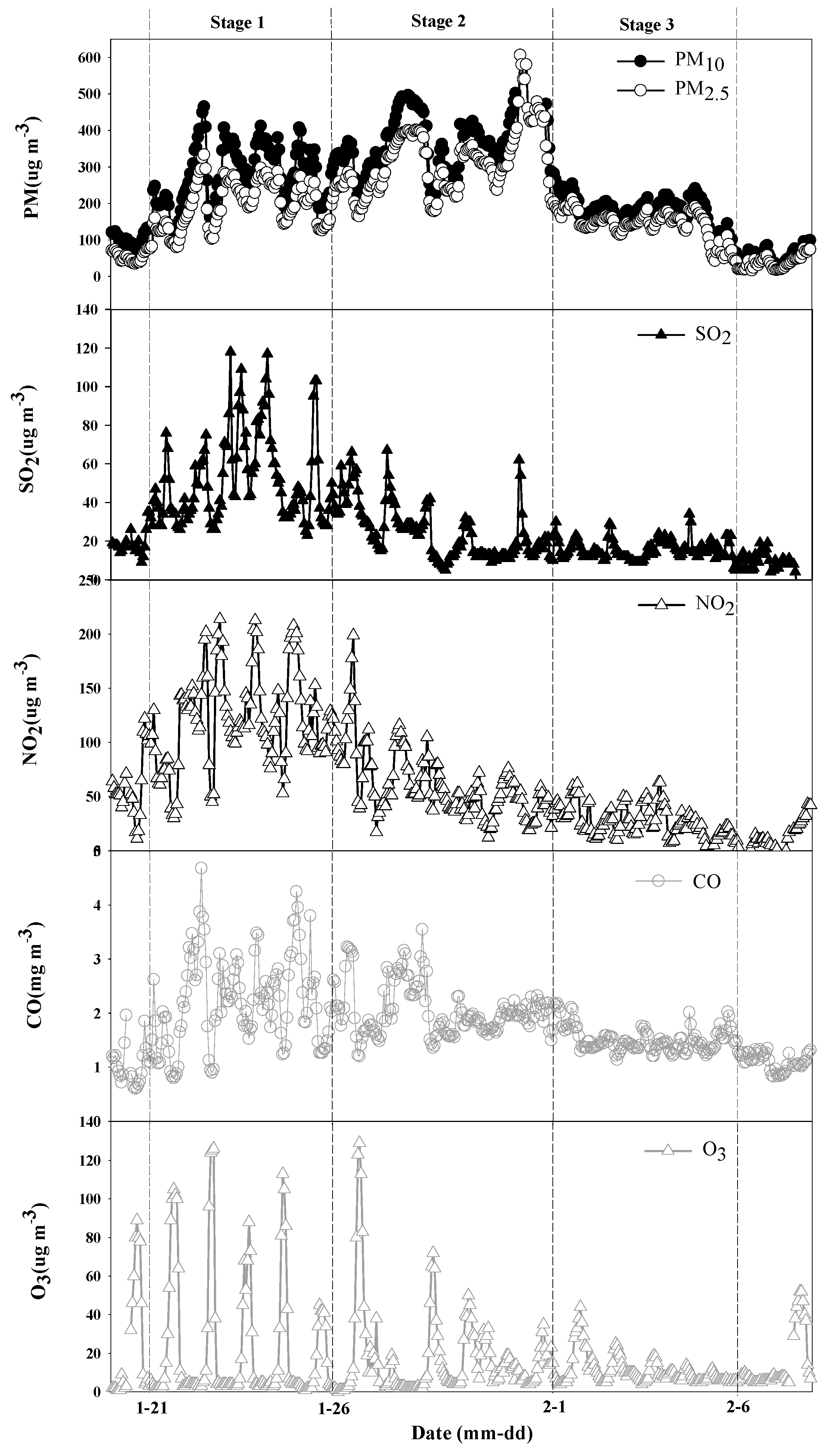
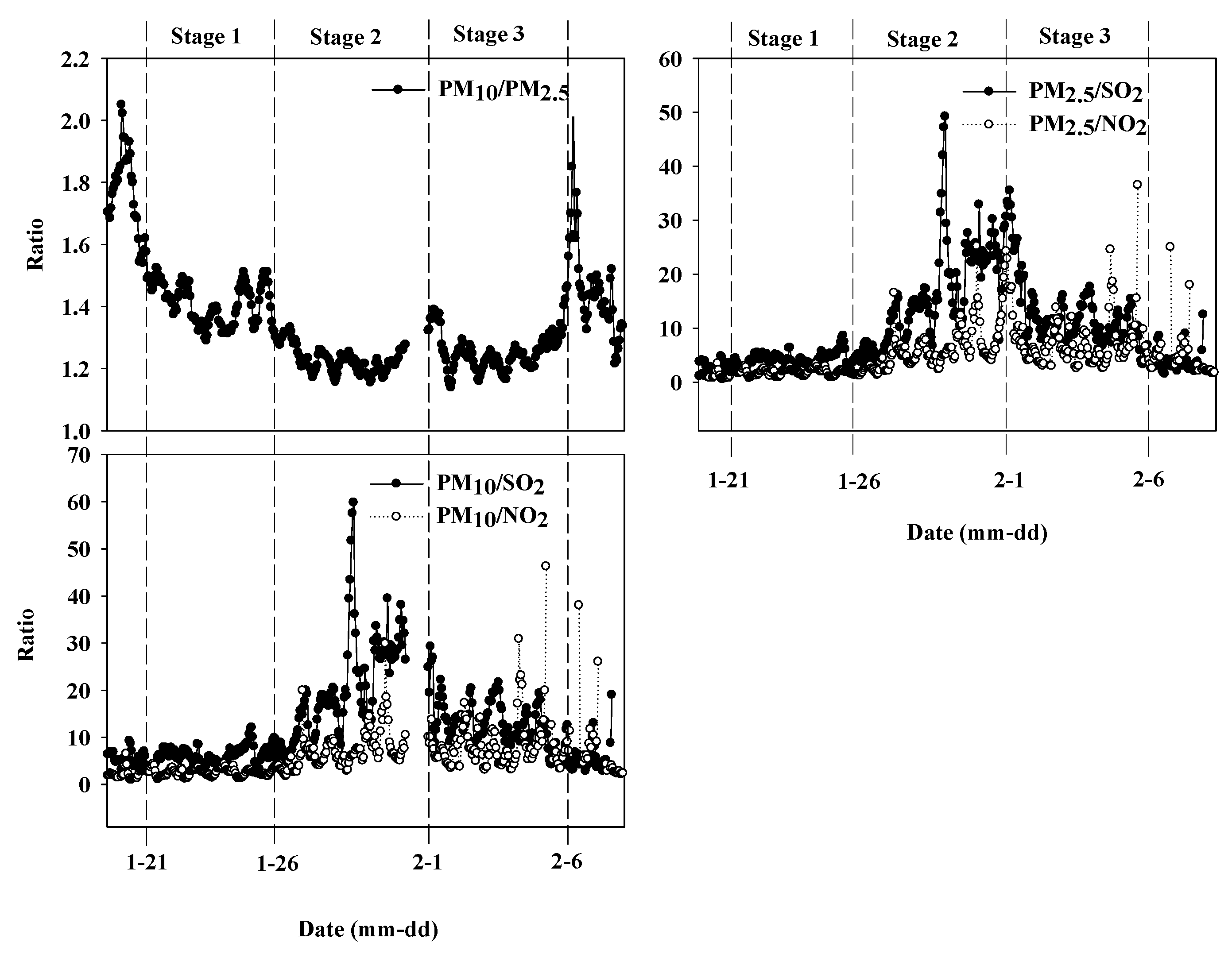
Figure 1 shows that from the 20th to the 22nd of January (within 30 h), the hourly mass concentration of PM10 increased from 80 to 449 μg m−3, with a high rate of increase of 12 μg m−3 per hour. The hourly mass concentration of PM2.5 increased from 43 to 325 μg m−3, with a high rate of increase of 9.4 μg m−3 per hour. At the same time, the hourly mass concentrations of SO2 and NO2 increased rapidly, up to 62 μg m−3 and 160 μg m−3, with a rate of increase of 1.5 μg m−3 and 4 μg m−3 per hour, respectively. The hourly mass concentration of PM2.5 ranged from 126 to 606 μg m−3 from the 23rd of January to the 1st of February, and the average hourly mass concentration was 289.5 μg m−3. A similar distribution pattern was found for PM10; its concentration ranged from 180 to 502 μg m−3, and the average hourly mass concentration was 341.0 μg m−3. The average hourly mass concentration of SO2 and NO2 was 52.9 and 122.9 μg m−3 from the 24th to the 26th of January, respectively, and their concentration then decreased from the 26th of January to the 1st of February, with an average hourly mass concentration of 24.5 and 60.5 μg m−3, respectively (Figure 1). A similar distribution pattern was found for CO and O3 (Figure 1). Figure 2 shows that some pollutants might transform into other pollutants during this event. From the 21st to the 26th of January, the average ratio between the hourly mass concentration of PM10 and PM2.5 was 1.43, and the ratio dropped to 1.24 from the 27th of January to the 5th of February. When considering the ratio between the hourly mass concentration of particulate matter (PM10 and PM2.5) and gaseous pollutants (SO2 and NO2), the ratio (PM2.5/NO2, PM2.5/SO2, PM10/NO2, and PM10/SO2) increased from the 26th of January to the 1st of February, and the ratio dropped slightly from the 2nd to the 5th of February (Figure 2). Both Figure 1 and Figure 2 suggest that the higher concentrations of particulate matter and the sudden drop of gaseous pollutants (SO2 and NO2) from the 26th of January to the 1st of February, might have resulted from a rapid transformation of the gaseous pollutants to particulate matter. Similar results were found by Wang et al. (2014), mainly caused by the fast secondary transformation of primary gaseous pollutants, such as SO2 and NO2, into secondary inorganic ions (sulphate and nitrate) [2]. When the relative humidity (RH) is below 35%, the majority of SO2 and NO2 remains unoxidized; when the RH is above 50%, most of the SO2 is oxidized into sulphate, and most of the NO2 has been oxidized into nitrate [2]. Figure 1 indicates that the increasing PM2.5/SO2 ratio was accompanied by a decrease in the PM2.5/NO2 ratio. It is possible that this can be explained by the new mechanism recently proposed for SO2 oxidation by NO2. The new mechanism suggests that aerosol water serves as a reactor, where the alkaline aerosol components trap SO2, which is oxidized by NO2 to form sulfate [36]. Wang et al. (2016) also show that the aqueous oxidation of SO2 by NO2 is key to efficient sulfate formation, but is only feasible under two atmospheric conditions: on fine aerosols with a high relative humidity and NH3 neutralization, or under cloudy conditions [37]. In this study, we also found an increasing relative humidity on the 27th of January. Figure 1 also implies that the diurnal variation of the ozone concentration was obvious. It is known that O3 is the secondary pollutant produced by the chemical reaction. It has a higher concentration when the solar radiation is strongest and the temperature is the highest (usually at 2–3 pm). Similarly, there were spikes in the ozone concentration after 2 pm in this study (Figure 1). Our unpublished research on the effect of solar radiation on the ozone concentration implies that there is a positive correlation between the ozone concentration and solar radiation. In this study, SO2 spikes were accompanied by NO2 and CO spikes; additionally, a high ozone concentration was observed, even though the particulate matter concentration was very high in haze pollution Stages 1 and 2 (Figure 1). This phenomenon may relate to the structure of the atmospheric boundary layer. When the atmosphere is neutral or stable, the diffusion is poor and is accompanied by a lower atmospheric mixed layer, impeding the spread of pollutants and increasing the concentration.
Therefore, when considering the concentration changes of the primary pollutant and the pollutant transformation process, this haze event during the spring festival in 2014 in Chengdu can be divided into three haze pollution stages. Haze pollution Stage 1 began on the 21st of January and ended on the 26th of January, representing the development process of the haze. Both the particulate matter and gaseous pollutants increased during Stage 1, and the average hourly mass concentrations of SO2, NO2, PM10, PM2.5, CO, and O3 were 51.6 μg m−3, 121.4 μg m−3, 275.9 μg m−3, 195.8 μg m−3, 2.2 mg m−3, and 22.6 μg m−3, respectively. Haze pollution Stage 2 was from the 27th of January to the 1st of February, and this stage was the evolution process of the haze. The particulate matters increased and gaseous pollutants decreased during this stage, and the average hourly mass concentrations of SO2, NO2, PM10, PM2.5, CO, and O3 were 24.5 μg m−3, 60.5 μg m−3, 359.0 μg m−3, 315.6 μg m−3, 2.0 mg m−3, and 17.0 μg m−3, respectively. Haze pollution Stage 3 was from the 2nd to the 5th of February, and this stage was the dissipation process of the haze, and both the particulate matter and gaseous pollutants decreased during this stage; the average hourly mass concentrations of SO2, NO2, PM10, PM2.5, CO, and O3 were 15.6 μg m−3, 26.6 μg m−3, 178.6 μg m−3, 143.3 μg m−3, 1.5 mg m−3, and 10.9 μg m−3, respectively.
3.2. Synoptic Circulation, Meteorological Conditions and Boundary Layer Structure during the Haze Event
3.2.1. Synoptic Circulation
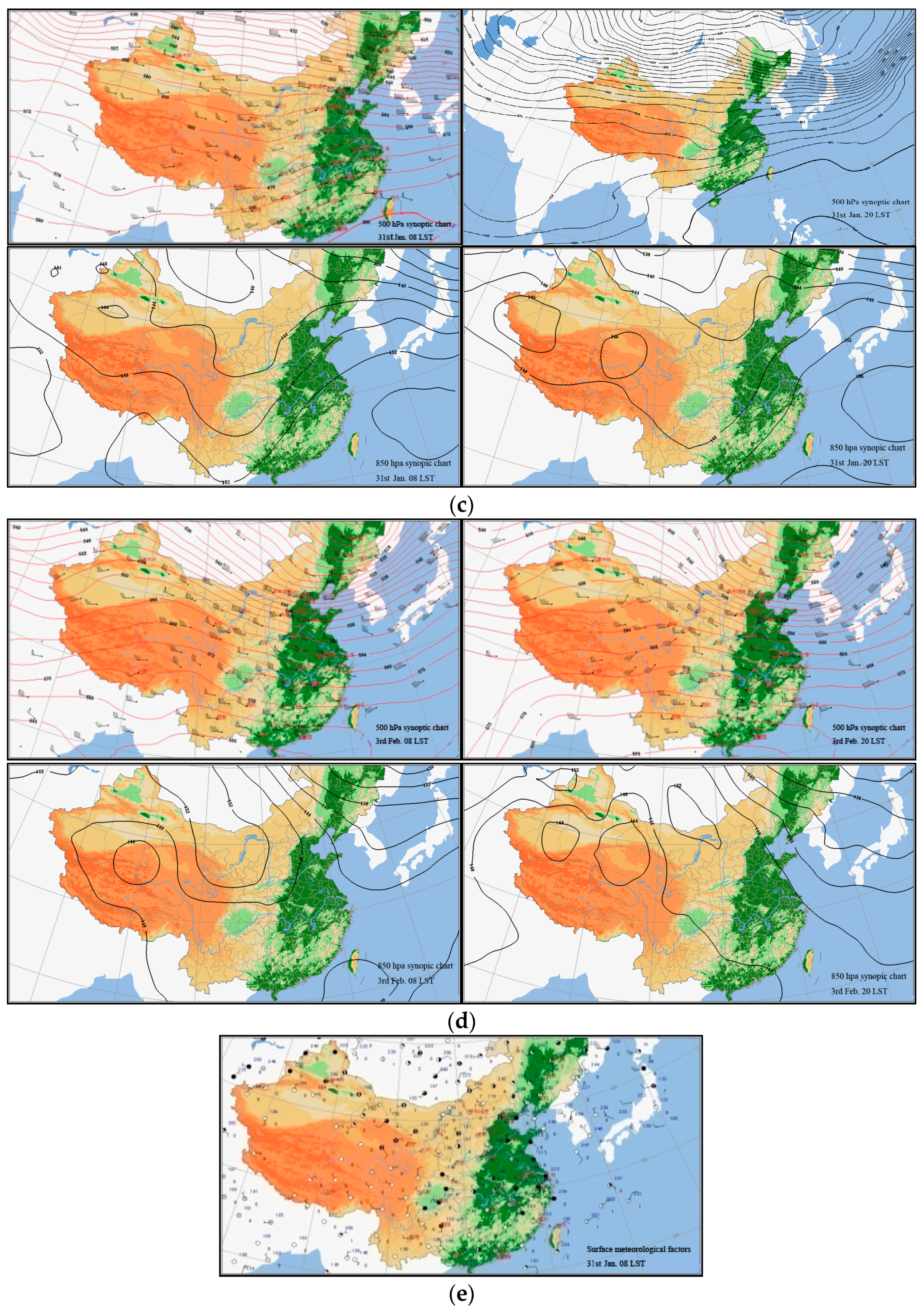
The Chengdu area was mainly under the control of Siberian high pressure from the 20th of January to the 7th of February, and the wind field was in a convergence condition during the majority of this time. During this event, a westerly flow prevailed, and zonal circulation dominated at a high altitude (500 hPa). The pressure field was stable and resulted in a lower pressure gradient and wind speed. Specifically, the circulation form was stable and less changed from the 22nd to the 26th of January, and a small trough transited this area. The circulation form was also stable from the 26th of January to the 4th of February, and a ridge transited the area at 20 LST (Local Standard Time) on the 4th of February (Figure 3). In the Chengdu area, a westerly zonal circulation was significant above 500 hPa at high altitude, and the 850 hPa isobar was sparse, which resulted in a small pressure gradient force, possibly having led to a lower wind speed (<2 m s−1, Figure 4). On the ground, this was often controlled by a high pressure and lower wind speed, which might have induced a poor diffusion condition (Figure 3). Thus, the pollutants could not have easily diffused in the horizontal and vertical directions; therefore, the poor circulation resulted in the accumulation of pollutants. The same results were found in other studies. Wang et al. (2011) suggest that the variation of PM2.5 was mainly controlled by the large scale synoptic system [12]. The concentration changes of pollutants in a regional air pollution process are subject to the impacts of atmospheric conditions, as the removal, accumulation, and convergence of air pollutants are closely related to the changes in weather patterns [20].
3.2.2. Meteorological Conditions at the Surface
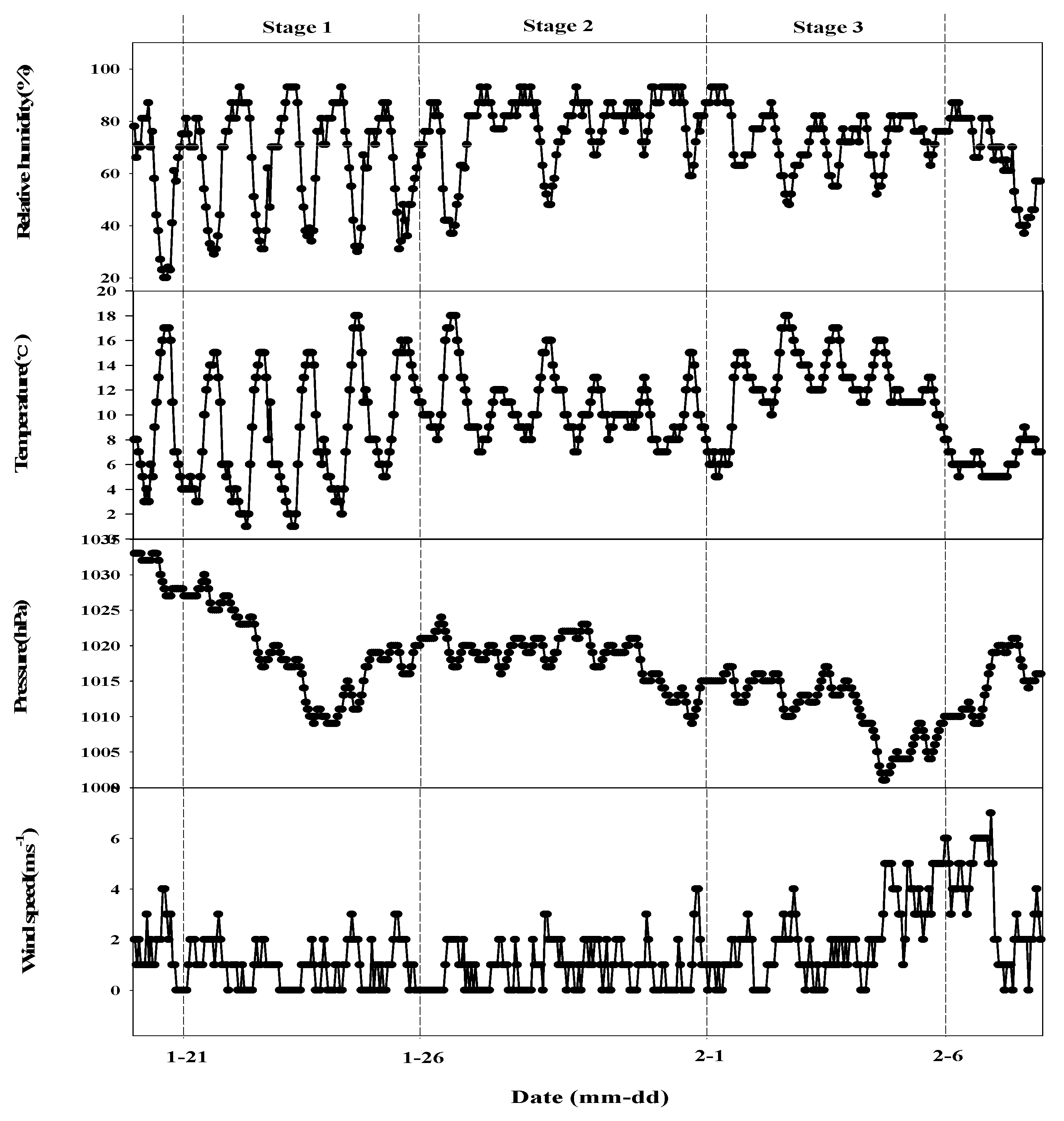
All of the meteorological elements considered in this study presented an obvious daily variation pattern (Figure 4). During haze pollution Stages 1 and 2 (development and evolution process), the wind speed was low (<2 m s−1), and it was usually (73%) below 1 m s−1. At the end of haze pollution Stage 3 (dissipation process), the wind speed increased to 4–6 m s−1 (Figure 4). During haze pollution Stage 1, the amplitudes of air temperature (ranged from 1 to 17 °C), relative humidity (ranged from 20% to 88%), and air pressure (ranged from 1009 to 1030 hPa) were high. During haze pollution Stage 2, the highest average air temperature was 13.9 °C, the temperature amplitude decreased compared to Stage 1, and the air temperature ranged from 8 to 16 °C. At the same time, the average highest relative humidity was 90%, and the relative humidity ranged from 60% to 93% (Figure 4). The average highest air pressure was 1022 hPa, and the air pressure ranged from 1016 to 1022 hPa. During haze pollution Stage 3, the average highest air temperature was 16 °C, and the air temperature ranged from 10 to 18 °C. At the same time, the average highest relative humidity was 85%, and the relative humidity ranged from 48% to 87% (Figure 4). For air pressure, the average highest air pressure was 1016 hPa, and the pressure ranged from 1001 to 1017 hPa. From the comparison of the metrological elements among the three stages, the amplitude of air temperature and relative humidity were low in the accumulation period of the pollutants. Simultaneously, the air temperature and wind speed were lower, and the relative humidity and air pressure were comparatively higher than for the pollutants dissipation process. Correlation analysis showed that the mass concentration of pollutants (PM10, SO2, NO2, CO) and temperature were inversely correlated and that the mass concentration of O3 and temperature were positively correlated (Table 2). There was a positive correlation between the mass concentration of the majority of pollutants (PM10, SO2, NO2, CO, O3) and pressure, and an inverse correlation was found between the concentration of all pollutants and wind speed. The mass concentration of PM2.5, PM10, and CO increased significantly with the increase in relative humidity (Table 2). The mass concentration of SO2 and NO2 decreased significantly with the decrease in the range of air temperature and relative humidity (Table 2). Figure 4 and Table 2 illustrate that the increased relative humidity or sustained high relative humidity and weak wind were the primary meteorological causes for the accumulation and preservation of haze pollution over the Chengdu area. In this study, we found that the concentration of SO2 and NO2 significantly decreased with the decrease in the range of air temperature and relative humidity, which meant smaller changes of air temperature and relative humidity. A higher relative humidity helped trigger the transformation of SO2 and NO2 to particulate matter and the hygroscopic growth of particulate matter in Stage 2; simultaneously, the lower air temperature resulted in less air mass motions, which might have impeded the dissipation of the particulate matter. There was a positive correlation between the concentration of SO2 and NO2 and the daily duration of sunshine. Many studies also suggest that increased air pollutant concentrations in the urban environment do not typically result from sudden increases in emission, but rather from meteorological conditions that impede dispersion in the atmosphere or result in increased pollutant generation [7,38,39,40]. Shen and Li (2016) showed that the coefficients between API and an atmospheric pressure anomaly, and precipitation and wind speed, are always negative at the studied time scales [10]. Wang et al. (2011) found that the concentration of PM2.5 and wind showed a certain negative relationship. For example, the concentration of PM2.5 was 100 μg m−3 with mild wind, and its concentration would decrease when the wind speed was greater than 2.0 m s−1 [12]. Wang et al. (2011) also found that low winds and a high humidity were not favorable to PM2.5 dispersion, and the mixing height and temperature curve had a more important impact upon pollution [12].
3.2.3. Atmospheric Boundary Layer
The height of the mixing layer during haze pollution Stages 1 and 2 was lower than that in Stage 3 for most time levels. The lower atmospheric mixed layer limited the vertical diffusion of the pollutants, and all pollutants showed higher concentrations in haze pollution Stages 1 and 2 (Figure 1). At 08 and 20 LST, the height of the mixing layer ranged from 200 to 600 m in Stages 1 and 2, increasing to a range of 600 to 1200 m, and then to 1200 m at the end of Stage 3 (Figure 5). The height of the mixing layer was higher at 14 LST, and it ranged from 1000 to 1500 m at Stages 2 and 3. The diurnal variation of the height of the mixing layer was obvious: the mixing layer height was low in the morning (08 LST) and evening (20 LST), and then increased, spiking at 14 LST, before decreasing. The diurnal variation of the height of the mixing layer led to similar unimodal changes for most of the pollutants, such as PM2.5, PM10, SO2, and NO2 (Figure 1).
In most cases, temperature inversion layers formed throughout the haze event, usually at 500 m to 4 km above the ground from the 24th of January to the 7th of February. Additionally, there were two or more inversion layers most of the time (Figure 5 and Figure 6). For example, two inversion layers formed at 20 LST on the 24th of January, and three to five inversion layers formed from the 25th of January to the 1st of February (haze pollution Stage 1 and 2). During haze pollution Stages 1 and 2 (corresponding to when the mass concentration of particulate matters was higher), the height of the bottom of the first temperature inversion layer ranged from 600 to 700 m above the ground (Figure 7 and Figure 1). Simultaneously, the intensity of the formed temperature inversion layer was stable and strong, ranging from 3 to 6 °C per 100 m (Figure 6). Specifically, during the period from the 27th to the 31st of January, the inversion layer was thick (with thickness of 0.7 to 2 km), and the temperature difference between the bottom and the top of the inversion layer was high (with the difference ranging from 4 to 10 °C). On the 26th of January, there were four continuous inversion layers in the boundary layer, and the thickness of each layer was less than 0.2 km, with the reverse temperature difference being less than 4 °C (Figure 7a). On the 31st of January, the thickness of the inversion layer was more than 0.8 km, and the reverse temperature difference was more than 6 °C, and at 20 that day, the reverse temperature increased up to 10 °C (Figure 7b). Both the particulate matter and gaseous pollutants decreased during haze pollution Stage 3 (from 2nd to 5th February), and there were two to four inversion layers formed at 2 to 4 km above the ground. The intensity of the formed inversion layer decreased compared to that in haze pollution Stages 1 and 2, ranging from 1 to 3 °C per 100 m (Figure 6). For example, the reverse temperature was 8 °C at 08, and the thickness of the inversion layer was 2 km at 20 on the 4th of February (Figure 7c). In general, there were one or more temperature inversion layers during the haze event in this area. Additionally, the inversion layer formed with a high frequency and strong intensity. Both the inversion layer that developed and the lower height of the mixing layer would have inhibited the vertical diffusion of the pollutants, resulting in their accumulation. Conversely, when there is no inversion layer or it formed higher above the ground, or its intensity is weak and the height of the mixing layer is higher, the pollutants could dissipate in a large space, and their concentration could decrease.
4. Conclusions
When considering the concentration changes of the primary pollutants and the pollutant transformation process, this haze event can be divided into three stages: Stage 1, the concentration of all pollutants increased; Stage 2, the concentration of gaseous pollutants decreased, while that of particulate matter increased; Stage 3, the concentration of all pollutants decreased. Atmospheric circulation that is not conductive to pollutant dispersion, unfavorable meteorological conditions, frequently formed inversion layers, and a low height of the mixing layer resulted in this haze.
1. The haze was controlled by high pressure or a weak pressure field near the ground, and the wind speed was low, which might have induced poor diffusion conditions, such that the pollutants could not easily diffuse in either the horizontal or vertical direction. The poor weather conditions resulted in the accumulation of high concentrations of pollutants.
2. The boundary layer structure played an important role on the vertical diffusion of the pollutants. There were one or more temperature inversion layers during the haze event in this area. The inversion layer formed with a high frequency and strong intensity, and the height of the mixing layer was low. All of these adverse boundary structures would inhibit the vertical direction diffusion of the pollutants, which might have resulted in the accumulation of the pollutants.
3. There was a positive correlation between the concentration of NO2, CO, PM10, and air pressure, meaning that the higher the pressure, the lower the increase in the convection rate of the air, which was not conducive to the diffusion of the pollutants. There was a negative correlation between the concentration of NO2, CO, SO2, and air temperature. The sunlight was weak and the duration of sunshine was short in the winter. Thus, the temperature was low, and the temperature inversion layer was stable, which might have inhibited the vertical diffusion of the pollutants. There was a negative correlation between the concentration of the pollutants and wind speed. Generally, the higher the wind speed, the greater the distance the pollutants will be transported, and the chance of air pollution is low. When the wind speed is lower, the opposite occurs, and the pollutants will accumulate. There was a positive correlation between the concentration of the pollutants and relative humidity. The mass concentration of SO2 and NO2 decreased significantly with the decrease in the range of air temperature and relative humidity.
Acknowledgments
This research work was supported by the National Science Foundation of China (grant No. 41505122), the Environmental Protection Science and Technology Projects of Sichuan province (grant No. 2013HBZX01), the Science and Technology support project (grant No. 2015GZ0238), and introduced talents start project of Chengdu University of Information Technology (No. KYTZ201429).
Author Contributions
Shenglan Zeng conceived and designed the study, analyzed the data, and wrote the paper; Yu Zhang contributed reagents/materials/analysis tools and modified the paper.
Conflicts of Interest
The authors declare no conflict of interest.
Appendix A

Table A1.
AQI category and health implications according to ambient air quality index (AQI) technical regulations (trial) (HJ 633-2012).
Table A1.
AQI category and health implications according to ambient air quality index (AQI) technical regulations (trial) (HJ 633-2012).
| AQI | Air Pollution Level | Health Implications |
|---|---|---|
| 0–50 | Excellent | No health implications. |
| 51–100 | Good | Few hypersensitive individuals should reduce outdoor exercise. |
| 101–150 | Lightly Polluted | Slight irritations may occur, individuals with breathing or heart problems should reduce outdoor exercise. |
| 151–200 | Moderately Polluted | Slight irritations may occur, individuals with breathing or heart problems should reduce outdoor exercise. |
| 201–300 | Heavily Polluted | Healthy people will be noticeably affected. People with breathing or heart problems will experience reduced endurance in activities. These individuals and elders should remain indoors and restrict activities. |
| 300+ | Severely Polluted | Healthy people will experience reduced endurance in activities. There may be strong irritations and symptoms and may trigger other illnesses. Elders and the sick should remain indoors and avoid exercise. Healthy individuals should avoid outdoor activities. |
References
- Wu, D.; Wu, X.; Li, F.; Tan, H.; Chen, J.; Cao, Z.; Su, X.; Chen, H.; Li, H. Temporal and spatial variation of haze during 1951–2005 in Chinese mainland. Meteorol. Sin. 2010, 68, 680–688. [Google Scholar]
- Wang, Y.; Yao, L.; Wang, L.; Liu, Z.; Ji, D.; Tang, G.; Zhang, J.; Sun, Y.; Hu, B.; Xin, J. Mechanism for the formation of the January 2013 heavy haze pollution episode over central and eastern China. Sci. China 2014, 57, 14–25. [Google Scholar] [CrossRef]
- Ilten, N.; Selici, A.T. Investigating the impacts of some meteorological parameters on air pollution in Balikesir, Turkey. Environ. Monit. Assess. 2007, 140, 267–277. [Google Scholar] [CrossRef] [PubMed]
- Zhang, N.; Lu, Z.; Guan, Y.; Zhao, Y. Analysis of weather element characteristics and air pollution status during continuous fog days in Liaoning. Meteorol. Environ. Res. 2011, 2, 7–9. [Google Scholar]
- Chang, D.; Song, Y.; Liu, B. Visibility trends in six megacities in China 1973–2007. Atmos. Res. 2009, 94, 161–167. [Google Scholar] [CrossRef]
- Che, H.; Zhang, X.; Li, Y.; Zhou, Z.; Qu, J.J.; Hao, X. Haze trends over the capital cities of 31 provinces in China, 1981–2005. Theor. Appl. Climatol. 2008, 97, 235–242. [Google Scholar] [CrossRef]
- Aidaoui, L.; Triantafyllou, A.G.; Azzi, A.; Garas, S.K.; Matthaios, V.N. Elevated stacks’ pollutants’ dispersion and its contributions to photochemical smog formation in a heavily industrialized area. Air Qual. Atmos. Health 2015, 8, 213–227. [Google Scholar] [CrossRef]
- Gorai, A.K.; Tuluri, F.; Tchounwou, P.B.; Ambinakudige, S. Influence of local meteorology and NO2 conditions on ground-level ozone concentrations in the eastern part of Texas, USA. Air Qual. Atmos. Health 2015, 8, 81–96. [Google Scholar] [CrossRef] [PubMed]
- Górka-Kostrubiec, B.; Król, E.; Jeleńska, M. Dependence of air pollution on meteorological conditions based on magnetic susceptibility measurements: A case study from Warsaw. Stud. Geophys. Geod. 2012, 56, 861–877. [Google Scholar] [CrossRef]
- Shen, C.H.; Li, C.L. An analysis of the intrinsic cross-correlations between API and meteorological elements using DPCCA. Phys. A Stat. Mech. Appl. 2016, 446, 100–109. [Google Scholar] [CrossRef]
- Squizzato, S.; Masiol, M. Application of meteorology-based methods to determine local and external contributions to particulate matter pollution: A case study in Venice (Italy). Atmos. Environ. 2015, 119, 69–81. [Google Scholar] [CrossRef]
- Wang, B.; Cheng, Y.; Liu, H.; Chai, F. A typical production and elimination process of particles in Beijing during early 2008 Olympic Games. Meteorol. Environ. Res. 2011, 2, 70–73. [Google Scholar]
- Wang, F.; Yan, F. Analysis of the low visibility and air pollution process in shanghai during December 14–15, 2006. Meteorol. Environ. Res. 2010, 1, 61–65. [Google Scholar]
- Ding, J.; Zhu, T. Heterogeneous reactions on the surface of fine particles in the atmosphere. Chin. Sci. Bull. 2005, 48, 2267–2276. [Google Scholar] [CrossRef]
- Shi, K.; Liu, C.Q.; Li, S.C.; Shi, K.; Liu, C.Q.; Li, S.C. Self-organized criticality: Emergent complex behavior in PM10 pollution. Int. J. Atmos. Sci. 2013. [Google Scholar] [CrossRef]
- Zhang, Z.; Zhang, X.; Gong, D.; Kim, S.J.; Mao, R.; Zhao, X. Possible influence of atmospheric circulations on winter haze pollution in the Beijing-Tianjin-Hebei region, northern China. Atmos. Chem. Phys. 2016, 16, 561–571. [Google Scholar] [CrossRef]
- Wu, S. Analysis of weather conditions for air pollution in Nanning with high index. J. Guangxi Meteorol. 2004, 25, 40–43. [Google Scholar]
- Ordónez, C.; Mathis, H.; Furger, M.; Henne, S. Changes of daily surface ozone maxima in Switzerland in all seasons from 1992 to 2002 and discussion of summer 2003. Atmos. Chem. Phys. Discuss. 2005, 5, 1187–1203. [Google Scholar] [CrossRef]
- Jacob, D.J.; Winner, D.A. Effect of climate change on air quality. Atmos. Environ. 2009, 43, 51–63. [Google Scholar] [CrossRef]
- Wei, P.; Ren, Z.; Su, F.; Cheng, S.; Zhang, P.; Gao, Q. Environmental process and convergence belt of atmospheric NO2 pollution in north China. Acta Meteorol. Sin. 2011, 25, 797–811. [Google Scholar] [CrossRef]
- Ulas, I.; Tayanç, M.; Yenigün, O. Analysis of major photochemical pollutants with meteorological factors for high ozone days in Istanbul, Turkey. Water Air Soil Pollut. 2006, 175, 335–359. [Google Scholar]
- Jones, A.M.; Harrison, R.M.; Baker, J. The wind speed dependence of the concentrations of airborne particulate matter and NOX. Atmos. Environ. 2010, 44, 1682–1690. [Google Scholar] [CrossRef]
- Lin, W.; Xu, X.; Zhang, X.; Tang, J. Contributions of pollutants from north China plain to surface ozone at the Shangdianzi GAW station. Atmos. Chem. Phys. 2008, 8, 5889–5898. [Google Scholar] [CrossRef]
- Korsog, P.E.; Wolff, G.T. An examination of tropospheric ozone trends in the northeaster 25 US (1973–1983) using a robust statistical method. Atmos. Environ. 1991, 25B, 47–57. [Google Scholar] [CrossRef]
- Greene, J.S.; Kalkstein, L.S.; Ye, H.; Smoyer, K. Relationships between synoptic climatology and atmospheric pollution at 4 US cities. Theor. Appl. Climatol. 1999, 62, 163–174. [Google Scholar] [CrossRef]
- Liu, C.-M.; Huang, C.-Y.; Shieh, S.-L.; Wu, C.-C. Important meteorological parameters for ozone episodes experienced in the Taipei basin. Atmos.Environ. 1994, 28, 159–173. [Google Scholar] [CrossRef]
- Xu, W.Y.; Zhao, C.S.; Ran, L.; Deng, Z.Z.; Liu, P.F.; Ma, N.; Lin, W.L.; Xu, X.B.; Yan, P.; He, X.; et al. Characteristics of pollutants and their correlation to meteorological conditions at a suburban site in the north China plain. Atmos. Chem. Phys. Discuss. 2011, 11, 4353–4369. [Google Scholar] [CrossRef]
- Xu, X.; Li, Q.; Zhang, X. Analysis of the weather conditions for a case of heavy pollution in Beijing. Meteorol. Mon. 2005, 33, 32–36. [Google Scholar]
- Rao, X.; Li, F.; Zhou, N.; Yang, K. Analysis of a large-scale haze over middle and eastern China. Meteorol. Mon. 2008, 34, 89–96. (In Chinese) [Google Scholar]
- Huang, Z. Analysis on heavy pollution weather and meteorology factor change in Urumchi city. Arid Environ. Monit. 2005, 19, 154–157. (In Chinese) [Google Scholar]
- Tang, G.; Zhang, J.; Zhu, X.; Song, T.; Münkel, C.; Hu, B.; Schäfer, K.; Liu, Z.; Zhang, J.; Wang, L.; et al. Mixing layer height and its implications for air pollution over Beijing, China. Atmos. Chem. Phys. 2016, 16, 2459–2475. [Google Scholar] [CrossRef]
- Chen, Y.; Luo, B.; Xie, S.-D. Characteristics of the long-range transport dust events in Chengdu, southwest China. Atmos. Environ. 2015, 122, 713–722. [Google Scholar] [CrossRef]
- Chen, Y.; Xie, S. Temporal and spatial visibility trends in the Sichuan basin, China, 1973 to 2010. Atmos. Res. 2012, 112, 25–34. [Google Scholar] [CrossRef]
- Qian, Y.; Giorgi, F. Regional climatic effects of anthropogenic aerosols? The case of southwestern China. Geophys. Res. Lett. 2000, 27, 3521–3524. [Google Scholar] [CrossRef]
- Nozaki, K.Y. Mixing Depth Model Using Hourly Surface Observations; Report 7053; USAF Environmental Technical Application Center: Scott AFB, IL, USA, 1973. [Google Scholar]
- Cheng, Y.; Zheng, G.; Wei, C.; Mu, Q.; Zheng, B.; Wang, Z.; Gao, M.; Zhang, Q.; He, K.; Carmichael, G.; et al. Reactive nitrogen chemistry in aerosol water as a source of sulfate during haze events in China. Sci. Adv. 2017, 2, 1–11. [Google Scholar] [CrossRef] [PubMed]
- Wang, G.; Zhang, R.; Gomez, M.E.; Yang, L.; Zamora, M.L.; Hu, M.; Lin, Y.; Peng, J.; Guo, S.; Meng, J.; et al. Persistent sulfate formation from London fog to Chinese haze. Proc. Natl. Acad. Sci. USA 2016, 113, 13630–13635. [Google Scholar] [CrossRef] [PubMed]
- Cheng, C.S.; Campbell, M.; Li, Q.; Li, G.; Auld, H.; Day, N.; Pengelly, D.; Gingrich, S.; Yap, D. A synoptic climatological approach to assess climatic impact on air quality in south-central Canada. Part II: Future estimates. Water Air Soil Pollut. 2006, 182, 117–130. [Google Scholar] [CrossRef]
- Cuhadaroglu, B.; Demirci, E. Influence of some meteorological factors on air pollution in Trabzon city. Energy Build. 1997, 25, 179–184. [Google Scholar] [CrossRef]
- Tasdemir, Y.; Cindoruk, S.S.; Esen, F. Monitoring of criteria air pollutants in Bursa, Turkey. Environ. Monit. Assess. 2005, 110, 227–241. [Google Scholar] [CrossRef] [PubMed]
Figure 1.
Variation of particle matter (PM10 and PM2.5) and gaseous pollutants (SO2, NO2, CO, and O3) in Chengdu during the period of the 2014 spring festival.
Figure 1.
Variation of particle matter (PM10 and PM2.5) and gaseous pollutants (SO2, NO2, CO, and O3) in Chengdu during the period of the 2014 spring festival.

Figure 2.
Variation of the ratio between major pollutants (PM10/PM2.5, PM2.5/NO2, PM2.5/SO2, PM10/NO2, and PM10/SO2) in Chengdu during the period of the 2014 spring festival.
Figure 2.
Variation of the ratio between major pollutants (PM10/PM2.5, PM2.5/NO2, PM2.5/SO2, PM10/NO2, and PM10/SO2) in Chengdu during the period of the 2014 spring festival.

Figure 3.
(a) 500 hPa and 850 hPa synoptic chart at 08 and 20 LST on the 24th of January; (b) 500 hPa and 850 hPa synoptic chart at 08 and 20 LST on the 26th of January; (c) 500 hPa and 850 hPa synoptic chart at 08 and 20 LST on 31st of January; (d) 500 hPa and 850 hPa synoptic chart at 08 and 20 LST on the 3rd of February; (e) surface meteorological factors at 08 LST on the 31st of January.
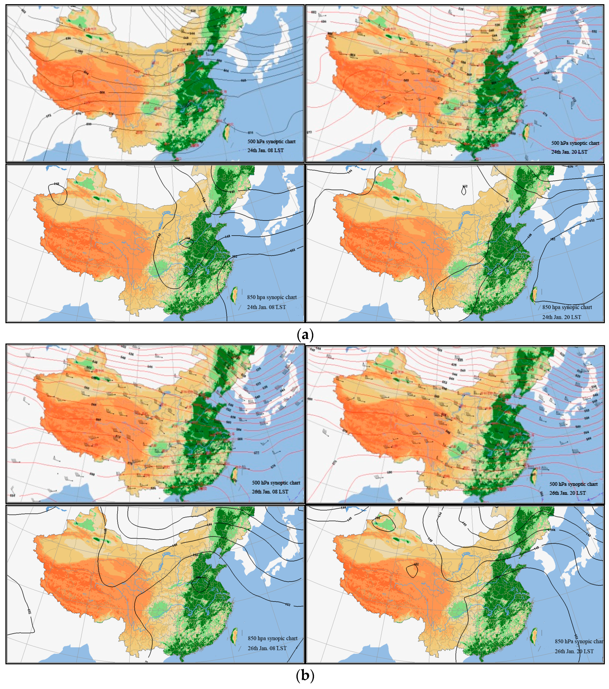

Figure 4.
The temporal variation of the meteorological variables in Chengdu during the 2014 spring festival at a one-hour time interval.
Figure 4.
The temporal variation of the meteorological variables in Chengdu during the 2014 spring festival at a one-hour time interval.

Figure 5.
The height of the mixing layer (m) in Chengdu among different haze stages at a time interval of 3 h.
Figure 5.
The height of the mixing layer (m) in Chengdu among different haze stages at a time interval of 3 h.
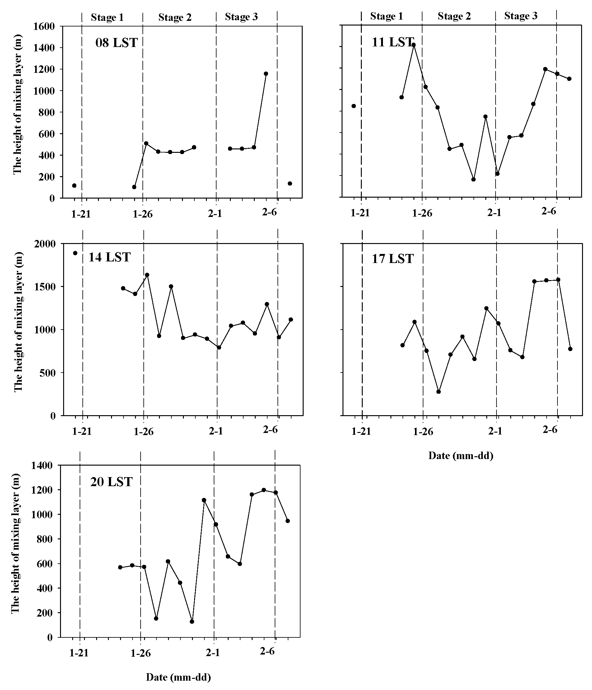
Figure 6.
The temporal variation of the height of the bottom and top of the first temperature inversion layer (m), and its intensity (°C per 100 m) in Chengdu during different haze stages at a time interval of 8 h.
Figure 6.
The temporal variation of the height of the bottom and top of the first temperature inversion layer (m), and its intensity (°C per 100 m) in Chengdu during different haze stages at a time interval of 8 h.
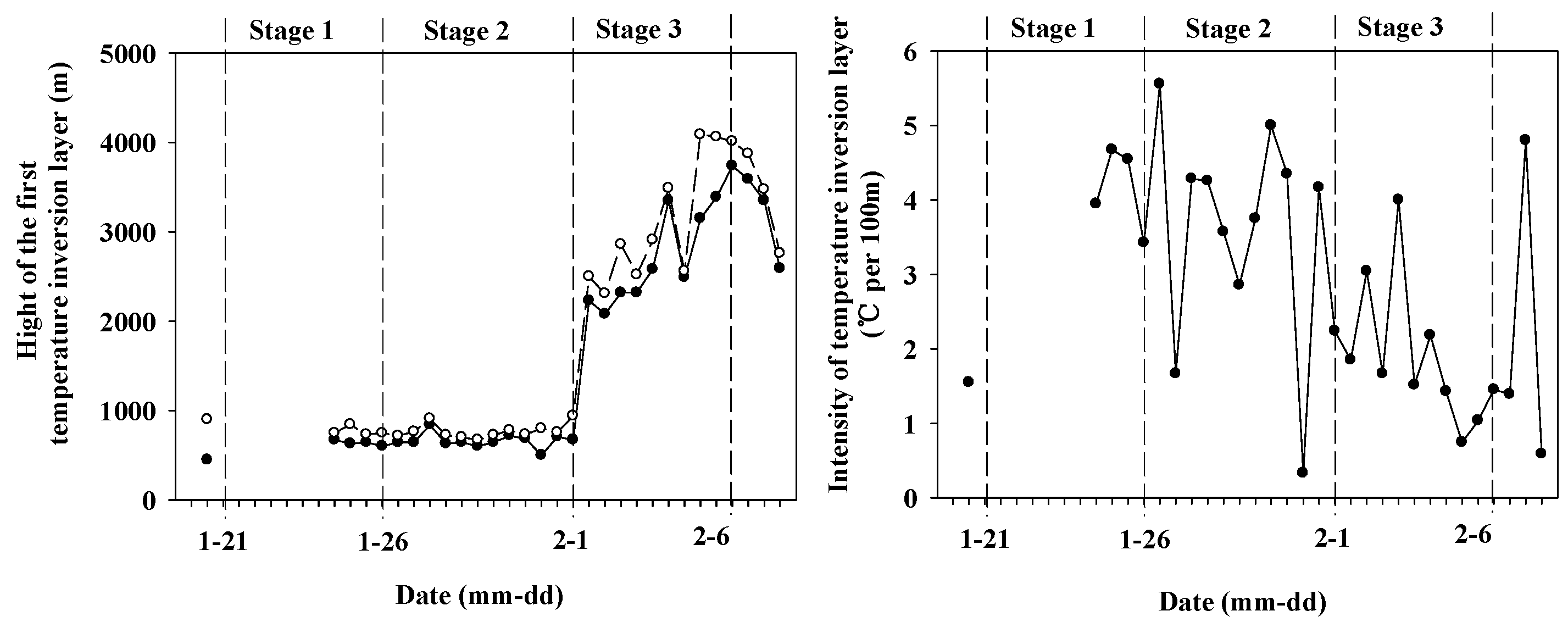
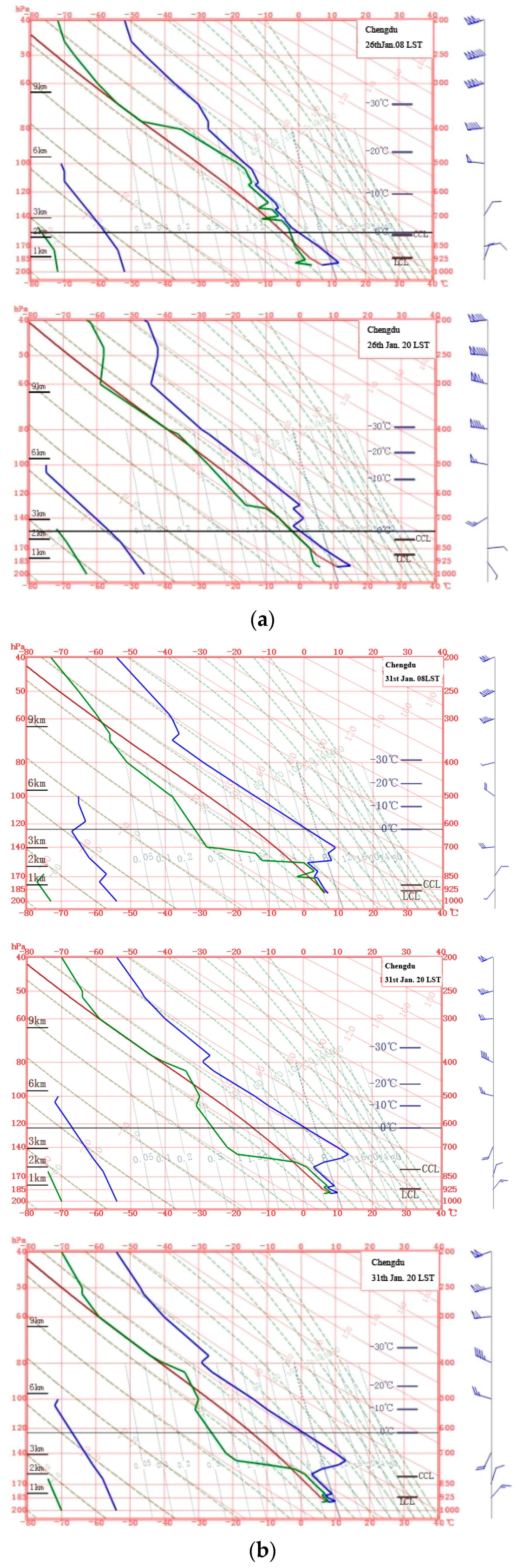
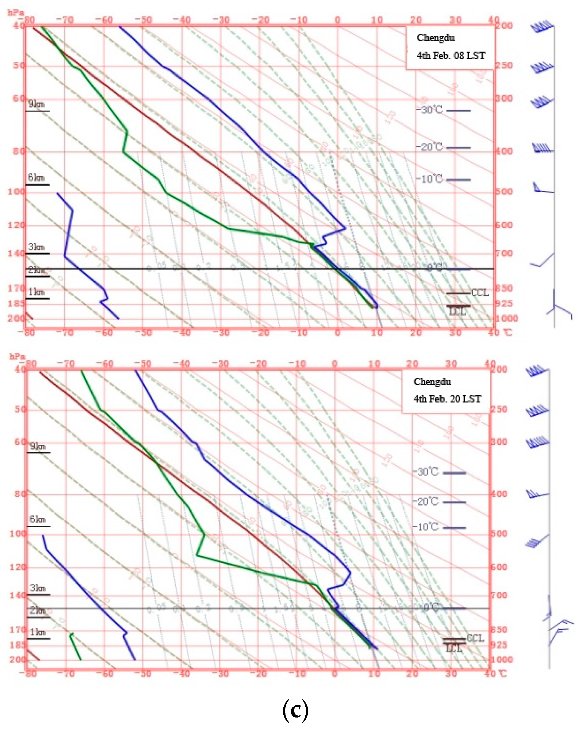
Figure 7.
(a) T-(-lnP) diagram at 08 and 20 LST on the 26th of January; (b) T-(-lnP) diagram at 08 and 20 LST on 31st of January; (c) T-(-lnP) diagram at 08 and 20 LST on the 4th of February. Horizontal axis and ordinate represent temperature (°C) and height (km), respectively. The blue curve on the far right of the graph represents the change of the temperature with height. Where the temperature increases with height (the slope below 90°), an inversion layer must exist.


Table 1.
Daily AQI and daily mass concentrations for PM2.5 (μg m−3), PM10 (μg m−3), SO2 (μg m−3), NO2 (μg m−3), CO (mg m−3), and O3 (averaged mass concentration for maximum 8 h, μg m−3) from the 20th of January to 7th of February according to the ground-based observation site.
Table 1.
Daily AQI and daily mass concentrations for PM2.5 (μg m−3), PM10 (μg m−3), SO2 (μg m−3), NO2 (μg m−3), CO (mg m−3), and O3 (averaged mass concentration for maximum 8 h, μg m−3) from the 20th of January to 7th of February according to the ground-based observation site.
| Date | SO2 | NO2 | PM10 | CO | O3 | PM2.5 | AQI | Air Pollution Level | Primary Pollutant |
|---|---|---|---|---|---|---|---|---|---|
| 1/20 | 19 | 74 | 111 | 1.2 | 63 | 62 | 93 | Good | NO2 |
| 1/21 | 39 | 93 | 198 | 1.4 | 86 | 125 | 165 | Moderate pollution | PM2.5 |
| 1/22 | 41 | 129 | 302 | 2.0 | 69 | 206 | 256 | Heavy pollution | PM2.5 |
| 1/23 | 63 | 132 | 356 | 2.4 | 66 | 254 | 304 | Severe pollution | PM2.5 |
| 1/24 | 49 | 124 | 325 | 2.1 | 65 | 236 | 286 | Heavy pollution | PM2.5 |
| 1/25 | 44 | 120 | 307 | 2.2 | 40 | 217 | 267 | Heavy pollution | PM2.5 |
| 1/26 | 38 | 104 | 306 | 2.0 | 83 | 233 | 283 | Heavy pollution | PM2.5 |
| 1/27 | 26 | 77 | 387 | 2.1 | 24 | 313 | 363 | Severe pollution | PM2.5 |
| 1/28 | 24 | 76 | 399 | 2.3 | 60 | 330 | 380 | Severe pollution | PM2.5 |
| 1/29 | 17 | 57 | 356 | 1.9 | 53 | 297 | 347 | Severe pollution | PM2.5 |
| 1/30 | 13 | 57 | 384 | 1.9 | 34 | 310 | 360 | Severe pollution | PM2.5 |
| 1/31 | 20 | 47 | 570 | 2.0 | 36 | 427 | 470 | Severe pollution | PM10 |
| 2/1 | 15 | 54 | 217 | 1.8 | 69 | 166 | 216 | Heavy pollution | PM2.5 |
| 2/2 | 17 | 43 | 179 | 1.5 | 75 | 146 | 195 | Moderate pollution | PM2.5 |
| 2/3 | 17 | 49 | 186 | 1.5 | 65 | 153 | 203 | Heavy pollution | PM2.5 |
| 2/4 | 21 | 39 | 205 | 1.6 | 54 | 168 | 218 | Heavy pollution | PM2.5 |
| 2/5 | 16 | 26 | 98 | 1.6 | 43 | 78 | 105 | Light pollution | PM2.5 |
| 2/6 | 11 | 25 | 43 | 1.2 | 34 | 28 | 43 | Excellent | - |
| 2/7 | 18 | 34 | 64 | 1.1 | 50 | 45 | 63 | Good | PM2.5 |
-: No primary pollutant.
Table 2.
The relationship between the mass concentration of air pollutants and the meteorological variables (Pressure = P, Temperature = T, Relative humidity = RH, Wind speed = WS, daily sunshine duration = SD, Range of temperature = Tr, Range of pressure = Pr, and Range of relative humidity = RHr).
| Pollutant | T | P | RH | WS | SD | Tr | Pr | RHr |
|---|---|---|---|---|---|---|---|---|
| PM2.5 | 0.005 | −0.008 | 0.41 ** | −0.47 ** | 0.13 | 0.17 | 0.03 | 0.16 |
| PM10 | −0.04 | 0.13 ** | 0.37 ** | −0.51 ** | 0.10 | 0.32 | 0.01 | 0.32 |
| SO2 | −0.11 * | 0.11 * | −0.06 | −0.27 ** | 0.65 ** | 0.78 ** | 0.25 | 0.63 ** |
| NO2 | −0.14 ** | 0.32 ** | −0.09 | −0.42 ** | 0.68 ** | 0.84 ** | 0.19 | 0.74 ** |
| CO | −0.22 ** | 0.10 * | 0.36 ** | −0.38 ** | −0.16 | 0.05 | 0.01 | 0.01 |
| O3 | 0.53 ** | 0.04 | −0.73 ** | 0.11 * | −0.16 | 0.02 | 0.03 | 0.06 |
* p < 0.05; ** p < 0.01.
© 2017 by the authors. Licensee MDPI, Basel, Switzerland. This article is an open access article distributed under the terms and conditions of the Creative Commons Attribution (CC BY) license (http://creativecommons.org/licenses/by/4.0/).
Share and Cite
MDPI and ACS Style
Zeng, S.; Zhang, Y. The Effect of Meteorological Elements on Continuing Heavy Air Pollution: A Case Study in the Chengdu Area during the 2014 Spring Festival. Atmosphere 2017, 8, 71. https://doi.org/10.3390/atmos8040071
AMA Style
Zeng S, Zhang Y. The Effect of Meteorological Elements on Continuing Heavy Air Pollution: A Case Study in the Chengdu Area during the 2014 Spring Festival. Atmosphere. 2017; 8(4):71. https://doi.org/10.3390/atmos8040071
Chicago/Turabian StyleZeng, Shenglan, and Yu Zhang. 2017. "The Effect of Meteorological Elements on Continuing Heavy Air Pollution: A Case Study in the Chengdu Area during the 2014 Spring Festival" Atmosphere 8, no. 4: 71. https://doi.org/10.3390/atmos8040071
Note that from the first issue of 2016, this journal uses article numbers instead of page numbers. See further details here.