
Application of Convective Condensation Level Limiter in Convective Boundary Layer Height Retrieval Based on Lidar Data


1
Key Laboratory of Arid Climatic Changing and Reducing Disaster of Gansu Province, Key Laboratory for Semi-Arid Climate Change of the Ministry of Education, College of Atmospheric Sciences, Lanzhou University, Lanzhou 730000, China
2
Center for Analysis and Prediction of Storms, and School of Meteorology, University of Oklahoma, Norman, OK 73072, USA
*
Author to whom correspondence should be addressed.
Atmosphere 2017, 8(4), 79; https://doi.org/10.3390/atmos8040079
Submission received: 6 January 2017
/
Revised: 18 April 2017
/
Accepted: 20 April 2017
/
Published: 23 April 2017
Abstract
:Micro pulse lidar is a promising tool for retrieving the convective boundary layer height (CBLH), but its application has been hindered by sharp extinction of the signal in high humidity conditions, e.g., clouds. To remedy this, we developed an effective and simple limiter to obtain more accurate estimates of the CBLH. The limiter is based on the algorithm for the convective condensation level (CCL) and is aimed at limiting the vertical extent of the lidar backscatter profile used in lidar methods to search for the CBLH. Four lidar methods (i.e., the gradient method, the idealized backscatter method, and two forms of the wavelet covariance methods) are used to calculate the CBLH with (or without) the limiter added. Compared to the CBLH calculated by the parcel method from microwave radiometer temperature data, more accurate retrieval of the CBLH is carried out with the limiter applied in four cloudy cases.
1. Introduction
The planetary boundary layer (PBL) is the turbulent mixing layer closest to the Earth’s surface, and it responds to surface forcings with a time scale of about an hour or less [1]. As it controls the interactions between the land surface and atmosphere and determines the air volume available for the dispersion of all atmospheric constituents, the PBL height is a key parameter in air quality control and pollutant dispersion studies.
Despite its importance, the PBL height cannot be directly measured. However, the concentration distribution characteristics of the substances in the mixed layer can be used to trace the top of the PBL. Under convective conditions, the convectively driven atmospheric boundary layer (CBL) is well mixed by vertical turbulent motion. This causes the wind speed, potential temperature, and atmospheric composition to have essentially no variation with increasing height within the boundary layer, while causing a significant increase in the wind speed and potential temperature or a decrease in the atmospheric composition at the top of boundary layer. Estimation of the convective boundary layer height (CBLH) thus relies on analysis of the vertical profiles of temperature, wind speed, or atmospheric composition [2,3,4,5,6]. Multiple methods based on data from different instruments have been used to extract boundary layer heights and often give varying results [7,8,9,10,11]. With the considerable number of ground-based lidar systems and lidar networks, e.g., EARLINET (the European Aerosol Research Lidar Network) [12], AD-net (the Asian dust and aerosol observation lidar network) [13], LALINET (Latin American Lidar Network) [14], and MPLNET (NASA Micro-Pulse Lidar Network) [15], the lidar approach is becoming increasingly important for tracing the boundary layer height by analyzing the vertical distribution of aerosols [16,17].
In lidar studies, the aerosol is used as a tracer. Generally, in convective boundary layers, aerosols often have sources at the surface, producing high concentrations in the mixed layer relative to the cleaner and drier free troposphere above. At the top of the mixed layer, there is a transition zone between the boundary layer and the free atmosphere, where cleaner and dryer air from the free atmosphere is entrained into the aerosol-laden moister boundary layer, called the entrainment zone. There are usually sharp gradients in the aerosol concentration through the entrainment zone at the top of the CBL. This characteristic can be used to retrieve the boundary layer height, and the use of lidar data for boundary layer retrieval has been described sufficiently in the literature [5,16,18,19,20,21,22,23,24,25,26].
Although lidar methods perform well in boundary layer height retrieval under clear sky conditions, such methods may fail under cloudy conditions, i.e., they are more likely to identify the “top” of the cloud as the boundary layer height because the strongest gradient in the signal will also occur in that part of the profile [21,27]. Thus, retrieval of the boundary layer height under cloudy conditions is poorly understood and very challenging. As we all know, the presence of clouds causes the altitude of the strongest humidity gradient to move higher in the entrainment zone [28,29]. On the other hand, in cloudy cases, free convection is not only driven by solar heating, but also by cloud-top radiative cooling. Thus, the presence of clouds influences the structure of the boundary layer. In the simplest case, the capping inversion prevents stratocumulus clouds from developing further, or the convective cloud development is limited under the convectively unstable atmospheric conditions, and the CBL is well mixed and fully coupled with clouds and sub-cloud layers. In such conditions, the cloud layer can be regarded as the upper portion of the boundary layer [1,27]. However, for continental boundary layers topped by cumulus clouds, the CBLH is distinct from the elevated cloud layers above the cumulus [30,31]. In such situations, clouds are not part of the boundary layer, and determination of the CBLH requires further consideration if we are to separate boundary layer clouds from clouds that are not part of the boundary layer.
It is therefore necessary to develop a cloud detection algorithm to differentiate cloud layers from the lidar profile. Several possible methods have been explored to address this issue. Some researchers use the change in the slope of the backscattered signal as a function of height to detect cloud layers and aerosol layers [19,32]. Others locate the cloud tops and bases by applying a threshold algorithm to the lidar profile [16,19,33], but this method is only well suited to cases in which the contrast in backscatter is very large [21]. Grimsdell and Angevine [28] used a ceilometer to measure cloud altitudes and developed a method of data selection to use the lifting condensation level (LCL) as an estimate of a reasonable range of cloud-base values. Some studies apply a continuous wavelet transform on lidar profiles to identify cloud or aerosol layers. Specifically, the wavelet coefficient has its minimum at the top and base of the cloud or advected aerosol layer and its maximum at their peaks. For example, Morille et al. [4] developed an automated algorithm combining a wavelet transform and thresholding to detect molecular layers (containing aerosols in small quantities) and particle layers (cloud layers and aerosol layers). Davis et al. [21] and Baars et al. [16] applied a Haar wavelet transform to distinguish the boundary layer from the cloud layers by altering the suitable wavelet dilation or by choosing a negative threshold. However, those techniques depend strongly on the vertical distribution of particle layers (aerosols and clouds) and are not suitable for dealing with complicated multiple-layer conditions [5,34].
In this paper, we present a simple algorithm based on a convective condensation level (CCL) limiter to deal with cloudy cases. The algorithm has the advantage that it may not be affected by the aerosol layers aloft. The limiter limits the vertical extent of the lidar signal profile used by lidar methods to search for the boundary layer top. Within this context, we explore the different lidar-based inversion methods of CBLH determination under cloudy cases. Section 2 briefly describes our measurement site, instruments, and data. The methods for boundary layer detection are described in Section 3, and results are discussed in Section 4. Section 5 presents our conclusions.
2. Measurement Site, Instruments and Data
The Semi-arid Climate Observatory and Laboratory of Lanzhou University (SACOL) was chosen as the site of focus for this study. The site is located 50 km southeast of the city of Lanzhou, in the suburban rural area of Lanzhou-Yuzhong (35.946° N, 104.137° E), at an elevation of 1961 m. The height of the CBL is retrieved using micro pulse lidar and microwave radiometer data. Micro pulse lidar is considered easier to use for its capability to operate unattended for long periods. It measures aerosols up to 20+ km, and provides great spatial and temporal resolution. The lidar signals used here have a vertical range resolution of 75 m and are stored at 1-min time intervals [35]. The raw lidar data are converted into Normalized Relative Backscatter (NRB) after being range-corrected and laser energy-normalized and having the background and dark count correction terms removed. Detailed procedures are discussed by Campbell et al. [36]. The data are also corrected for overlap with a full overlap height of about 6.45 km. Several methods have been used to determine the profile of the overlap factor [37,38,39,40,41]. Our overlap correction is determined by experimental methods such as those described by Sasano et al. [37]. The final variable NRB can be expressed as [42]:
where is the lidar constant, is the backscatter coefficient, and is the integral of the extinction coefficients from to . Since the CBL top is characterized by a sharp decrease in concentrations of passive constituents (e.g., aerosols and gases), the absolute minima in the vertical gradient of the lidar signal profile can be associated with the CBL top.
Temperature measurement in the lower atmosphere is achieved with the use of a ground-based microwave radiometer (TP-WVP3000). The TP-WVP3000 provides the atmosphere temperature ( profile between 0 and 10 km. The vertical resolution decreases with altitude, i.e., 100 m within 1 km and 250 m from 1 km up to 10 km. The time resolution is set to one profile every minute. For details about the instrument, see Ware et al. [43]. Microwave radiometer profilers have proven to be very appealing for boundary layer research because of their high temporal resolution and ability to operate unattended for long periods in nearly all weather conditions [44]. From the observed temperature profile, the CBLH is determined by applying the parcel method [2,5,29,45]. The method defines the CBLH as the height at which the dry adiabatic line starting at the surface intersects the actual temperature profile. Section 3.2 gives a description of the method in more detail. The parcel method depends strongly on the surface temperature [7]. The surface temperature retrieved from microwave radiometer observations is corrected by the surface temperature observed from a temperature and humidity sensor embedded in the TP-WVP3000 [46], and the measurement accuracy of surface temperature is 0.5 K. The boundary layer estimation based on such data using the parcel method has been achieved by Wang et al. [47].
3. CBLH Detection Methods
In this section, we describe the methods for determining boundary layer height from micro pulse lidar data (Section 3.1) and microwave radiometer temperature data (Section 3.2). Note that the lidar NRB profiles are averaged over a time period of 11 min, which not only takes the time variability of the boundary layer height into consideration but also helps to improve the signal-to-noise ratio.
3.1. Methods for Estimating the CBLH from Lidar Backscatter Data
Four commonly employed lidar methods (the gradient method, the idealized backscatter method, and two forms of wavelet covariance methods) were applied to retrieve the CBLH. The lidar methods are based on the assumption that aerosols are much more abundant within the boundary layer than in the free troposphere. Thus, the CBL tops can be characterized by a gradient in the NRB as a function of height.
The first adopted method for CBLH determination is called the gradient method (hereafter GM) [18,48]. This method is based on the calculated gradient of the NRB profile, and the gradient is expressed as:
A sharp decrease in the concentrations of aerosol between the mixed layer and the free atmosphere above corresponds to the abrupt decrease in the NRB signal, so the altitude corresponding to the maximum of indicates the CBLH.
The idealized backscatter method [20,49], also known as curve fitting (hereafter fitting), aims to fit a four-parameter ideal profile to the observed backscatter profile,. The ideal profile is expressed as:
where and are the average NRB values for the mixed layer and the free troposphere, respectively. The parameter is related to the entrainment zone thickness (), and, according to Steyn et al. [20], 2.77 times the value of is equal to the ; is the candidate CBLH, which is defined as the center of the ; and the error function is defined as . In the idealized backscatter method, the optimal value of that minimizes the is regarded as the real CBLH. Since fitting uses the whole NRB profile as a single shape, it can tolerate more signal noise than other lidar methods.
In addition to the basic gradient method and the idealized backscatter method, two wavelet methods were also used for CBLH determination. Measurement of the boundary layer height by the Haar wavelet method (hereafter referred to as the HM) makes use of coefficients of a Haar continuous wavelet transform of the backscatter profile. The Haar wavelet is defined as:
where is the translation of the Haar wavelet and is the wavelet dilation. The dilation equals , , ( corresponds to the vertical resolution of the lidar data), and the optimum value for is equal to the depth of the transition zone, which should be tested before being used. The HM allows a comparison between the NRB and the Haar wavelet, and the similarity between them can be measured by the wavelet coefficient :
where and are the floor and ceiling of the integral, respectively. The Haar coefficient, , presents the maxima when the translation of Haar wavelet coincides with the CBLH. The method is well suited to recognize a step function and has been adopted by other investigators and applied in several studies [17,34,50]. Similarly, the Mexican hat wavelet method (hereafter referred to as the MHM) allows a comparison between the NRB gradient () and the Mexican hat wavelet. The Mexican hat wavelet [51] is defined as:
The parameter , where the wavelet coefficient is at a maximum, coincides with the CBLH. For the two types of wavelet methods, the selection of an appropriate value for the wavelet dilation, , is the main challenge for a successful retrieval of the CBLH with the wavelet covariance transform method. Two cases (a clear-sky and cloudy case) are presented in Section 3.1 to show how the value of affects the resulting CBLH. In order to obtain more precise empirical initial values for the two wavelet methods, the lidar data used in this study have been interpolated to a vertical range resolution of 15 m using Lagrange linear interpolation.
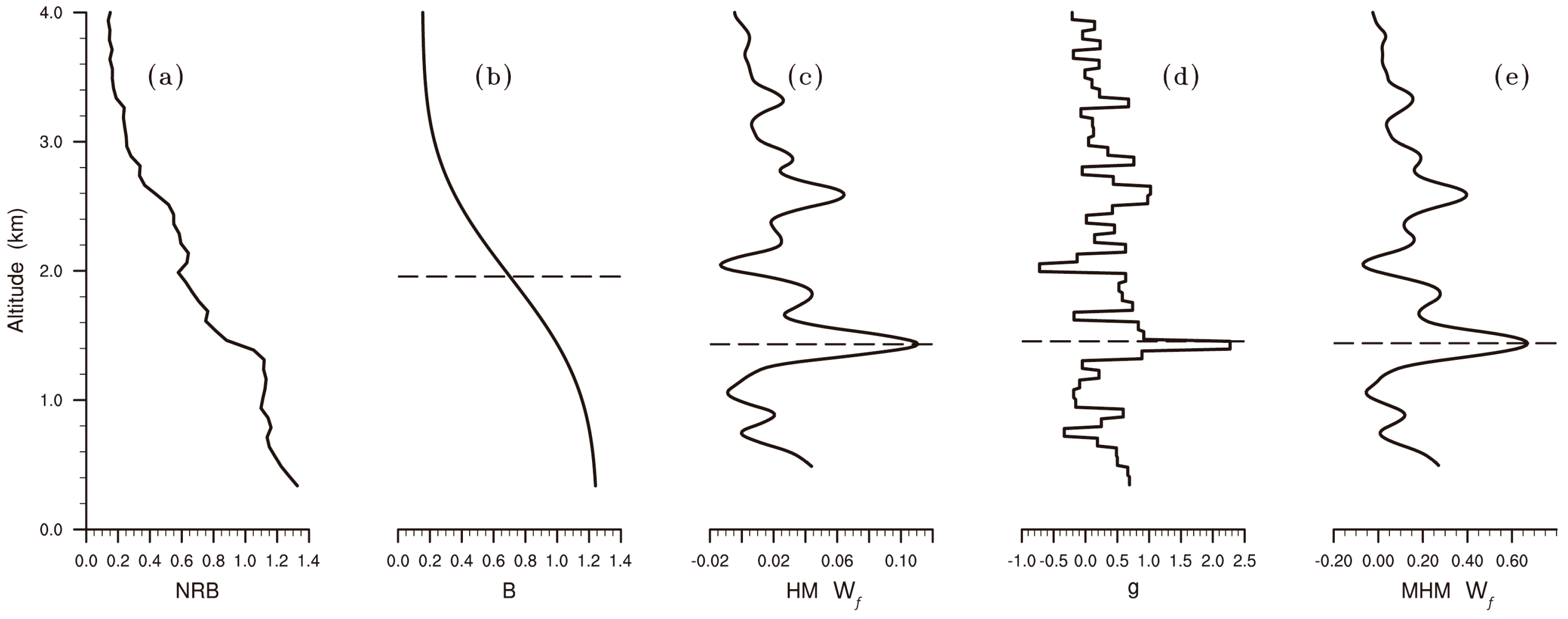
The NRB profile at 13:00 local time on 23 July 2007 was taken as an example to explain how these lidar methods work (See Figure 1). The CBL tops obtained by different methods are 1.455 km (GM), 1.9562 km (fitting), 1.4325 km (HM), and 1.440 km (MHM). The abrupt decrease in lidar NRB signal is designated as the CBL top and can be automatically captured by the HM (Figure 1c). Meanwhile, the significant signal loss at the height of the CBL top corresponds to the maximum of the signal gradient profile , which has the same shape as the Mexican hat wavelet function. For the two wavelet methods described above, reaches a local maximum at the height of the CBL top.
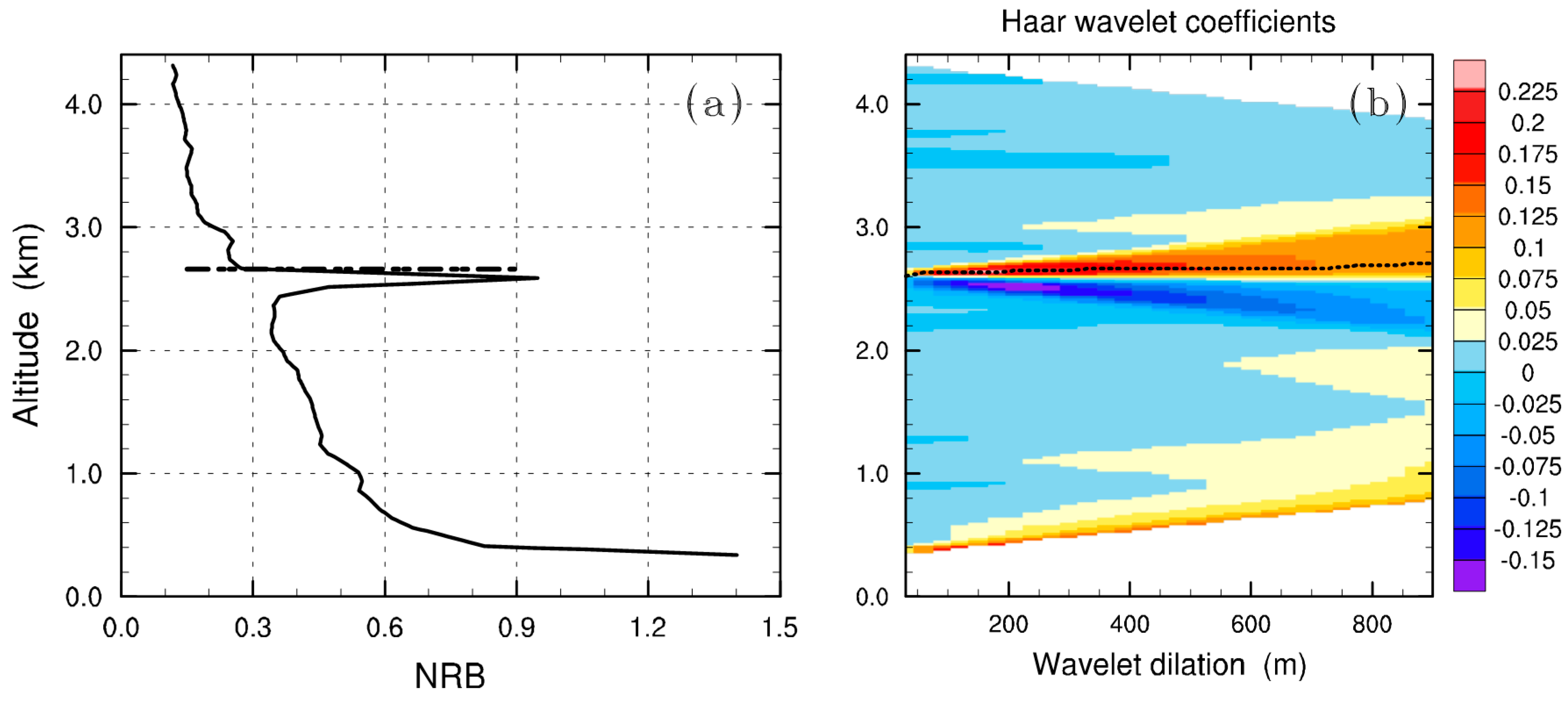
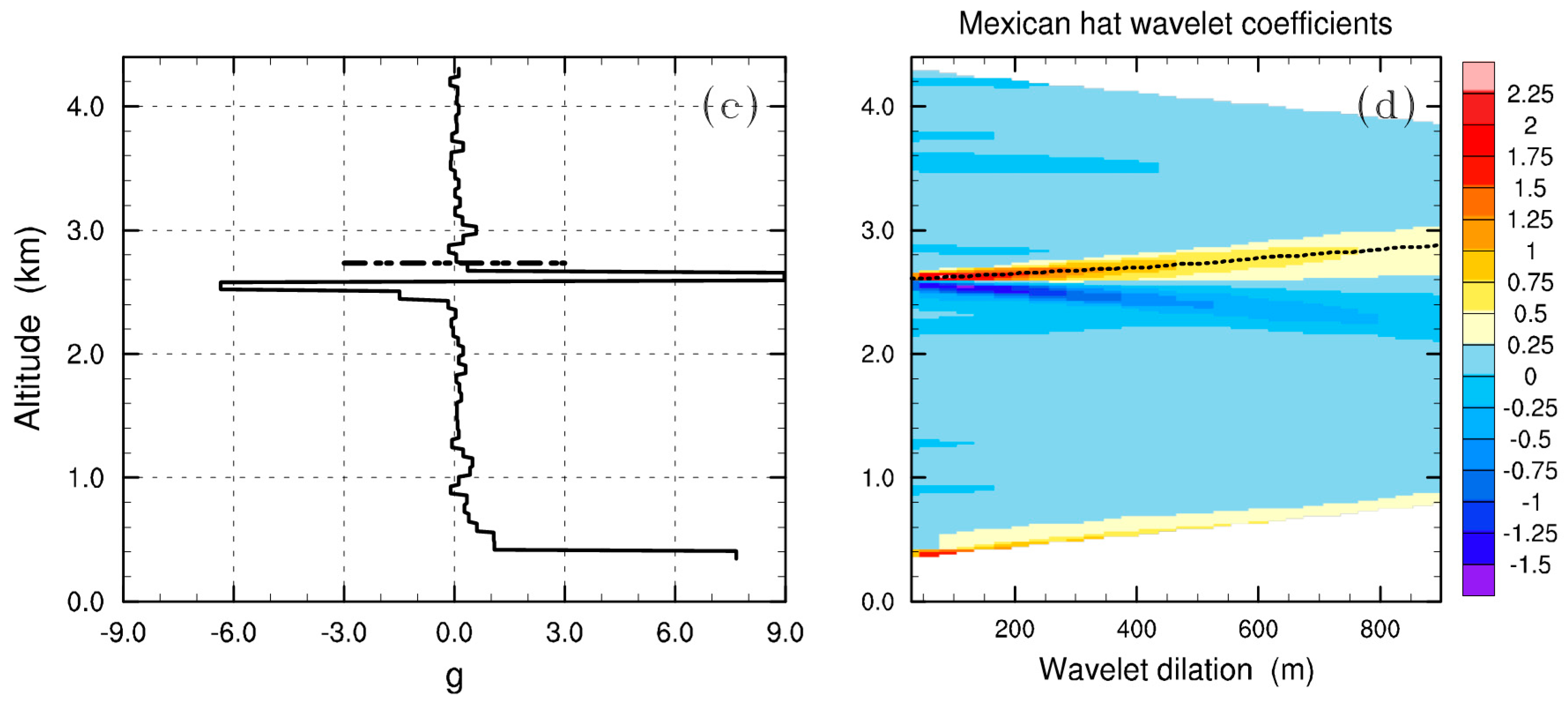
Different values of may generate different CBLH values with the wavelet methods. In order to verify the resulting CBLH with varying values of , two cases including a clear-sky case (Figure 2) and a cloudy case (Figure 3) were used to investigate the behavior of the two methods. The wavelet transform is simple to implement to recognize the scale of the identified feature. In Figure 2, in the clear-sky case, the average CBLH (the horizontal dotted line in Figure 2a) obtained by HM with different wavelet dilations is 1.4415 km. Meanwhile, the average CBLH (the horizontal dotted line in Figure 2c) obtained by HMH with different wavelet dilations is 1.461 km, which is near the altitude where the maximum of occurs. The study of the clear-sky case shows that both wavelet methods provide robust means of deriving the CBLH. The similar CBL tops are obtained with different scales, i.e., different wavelet dilations are used for the lidar data. However, for the cloudy NRB profile, the NRB signal does not decrease with increasing height as in typical NRB profiles but has an abrupt increase caused by clouds (around 2.4–2.6 km in Figure 3a), followed by a sharp decrease in the signal at the top or edge of the cloud. The corresponding characteristic in is that a minimum is reached at the cloud base, followed by a maximum at the cloud top or edge (Figure 3c). This characteristic of the signal at the cloud top or edge is similar to that at the CBL top. Thus, the real CBL top is replaced by the cloud top even if different wavelet dilations are used.
3.2. Methods for Estimating the CBLH from Microwave Radiometer Temperature Data
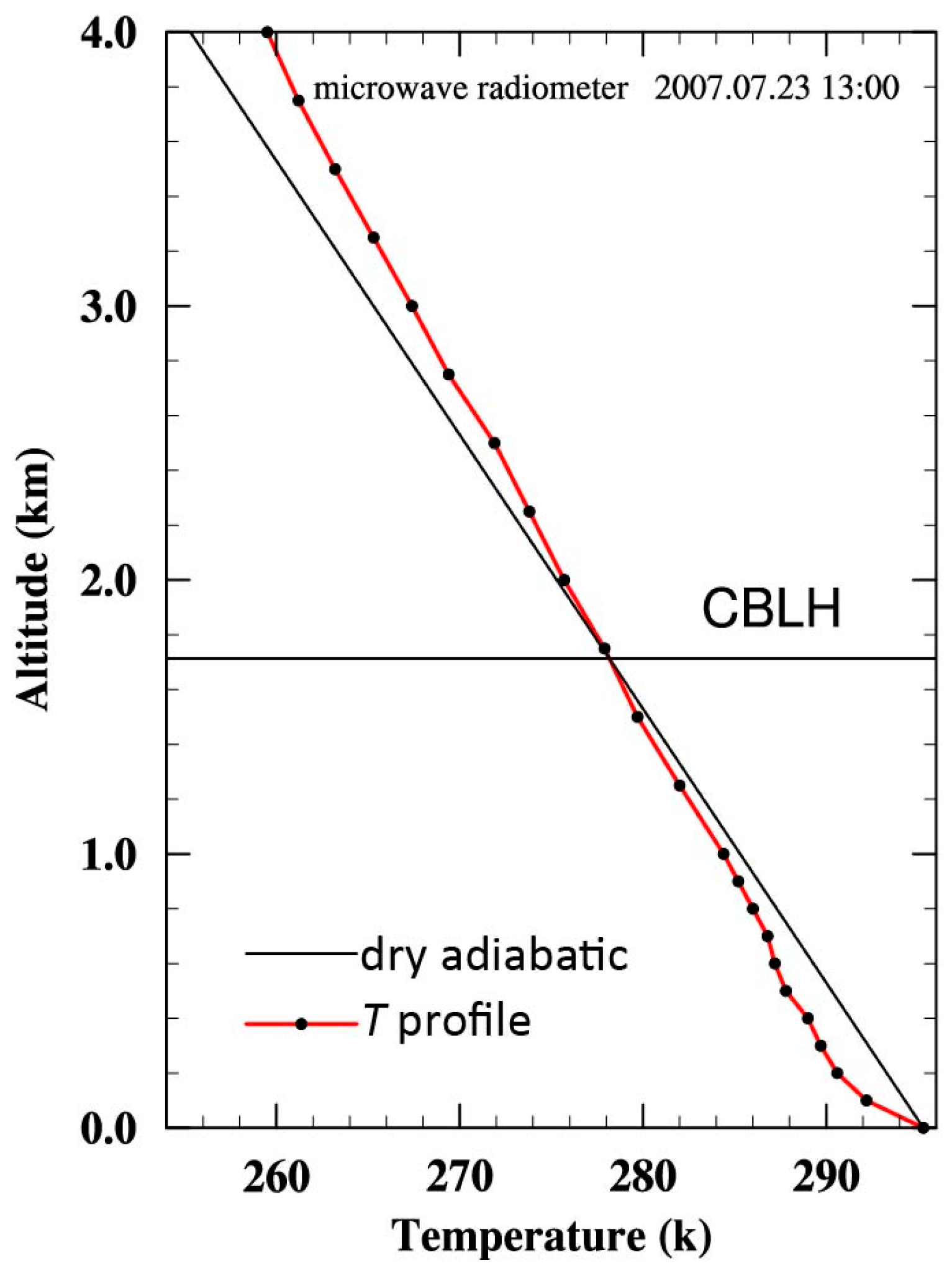
The parcel method is applied to the microwave radiometer profile to detect the CBLH. It defines the CBLH as the height at which an air parcel rising dry-adiabatically from the surface intersects the actual temperature profile [2]. An example of CBLH retrieval using this method is shown in Figure 4, and the resulting CBLH is 1.7140 km.
3.3. Convective Condensation Level Limiter
In Section 3.1, we find that the CBLH retrieved by the wavelet methods is often unrealistic in cloudy cases because the decrease in the backscatter signal at the cloud top or edge is similar to the decrease at the boundary layer top. Therefore, the retrieved boundary layer height is always replaced by the cloud “top”. As clouds are characterized by a steep increase in the NRB at the cloud base, the cloud base can be identified as the altitude at which the Haar wave coefficient is lower than a chosen negative threshold [16,34]. In such studies, the signal values below the cloud base are then used only to determine the CBLH. However, what cannot be ignored is that when multiple aerosol layers exist, the aerosol layer may be mistakenly identified as the cloud. Here, we apply a simple technique to distinguish the boundary layer clouds from clouds above the boundary layer. The technique is based on knowledge of cloud formation and thus is not affected by aerosol layers aloft. Clouds can form at the top of the mixed layer, i.e., boundary layer clouds [1]. For a boundary layer topped by boundary layer clouds, the cloud top coincides with the height at which turbulence stops, and boundary layer height detection is aided by the sensitivity to clouds. However, for clouds above the boundary layer, the cloud top is significantly different from the CBLH, and it is difficult to extract the information needed to define the CBLH from the backscatter profile [30].
Consequently, we need to develop the ability to distinguish clouds that are not part of the boundary layer from the boundary layer clouds. It is well known that the formation of clouds depends on both dynamic and thermodynamic uplifts. When there is only mechanical forcing, the air being lifted dry-adiabatically will become saturated by adiabatic cooling and then condense into clouds at a certain height. This approximates the lifting condensation level (LCL). However, without mechanical lift, strong heating continues at the surface, and this heat will be transported upwards by convection. Clouds will form at the height at which the convective temperature is reached. This height is the convective condensation level (CCL). The base of the cumulus clouds occurs at the CCL [52]. The CCL is always higher than or equal to the LCL, and the LCL has long been used to estimate boundary layer cloud heights in convective conditions [53]. Therefore, the actual boundary layer cloud base height is considered lower than the CCL. That means clouds below the CCL are regarded as boundary layer clouds, whereas clouds above the CCL are not part of the boundary layer. As clouds above the CCL appear as sharp backscatter gradients in the lidar profile and lead to false diagnosis of the CBLH, the CCL is added as an upper limit (hereafter called the CCL limiter) to the algorithms of the lidar methods used here. That is, for lidar profiles with clouds above the CCL, only the NRB values below the CCL are used to determine the CBLH.
The LCL and CCL values used here are calculated using the temperature data from the microwave radiometer. As the LCL is defined as the intersection of the saturation mixing ratio line starting at the surface dew point temperature and the dry adiabatic lapse rate line starting at the surface temperature, it can be calculated using surface data and the following formula [54]:
where is the surface temperature from the microwave radiometer and is the dew point temperature of the surface, calculated by combining the surface temperature and relative humidity data from the microwave radiometer.
The CCL is set to the altitude at which the temperature profile crosses the saturation mixing ratio line that starts from the surface dew point temperature, but it is worth noting that this method assumes that the parcel ascends in an unsaturated condition until it reaches the CCL. However, in the early morning during autumn and winter, saturation condensation always occurs near the surface because of surface long-wave radiation cooling. To avoid the influence of this saturation condensation, the intersection that indicates the CCL is identified from the top downwards.
4. Results and Discussion
In this section, four cloudy cases (22 May, 9 June, 12 June, and 28 October 2007) were chosen to investigate how clouds influence CBLH retrieval, as well as how to obtain reliable CBLH values under cloudy conditions. The CBLH estimated by the parcel method based on microwave radiometer temperature data is regarded as the reference.
Figure 5 shows four cloudy cases. Clouds in each plot are indicated by the white portion with complete reduction above it. It is well known that if the cloud is part of the boundary layer structure, the cloud is coupled with the boundary layer top, causing turbulence mixing in boundary layer and resulting in the NRB values below the cloud base being able to remain high. Thus, considering the vertical distribution of NRB values and NRB values below but near the cloud base, clouds in our cases were not part of the boundary layer for most of the cloudy periods. However, for the cloud existing from 10:05 to 10:35 local time on 28 October 2007, the NRB values below the cloud are still high, so the cloud is identified as the boundary layer cloud. In our technique, the cloud is located between the LCL and CCL. Fortunately, from the LCL and CCL calculated each day at 10-min intervals (the LCL and CCL are calculated every minute and averaged every 11 min, shown as red and black solid lines in Figure 5, respectively) from 08:05 to 19:55, the cloud regarded as the boundary layer cloud based on the NRB values is between the LCL and the CCL. Meanwhile, the cloud portions at most other times are higher than the CCL. This in turn verifies that clouds above the CCL are not part of the boundary layer.
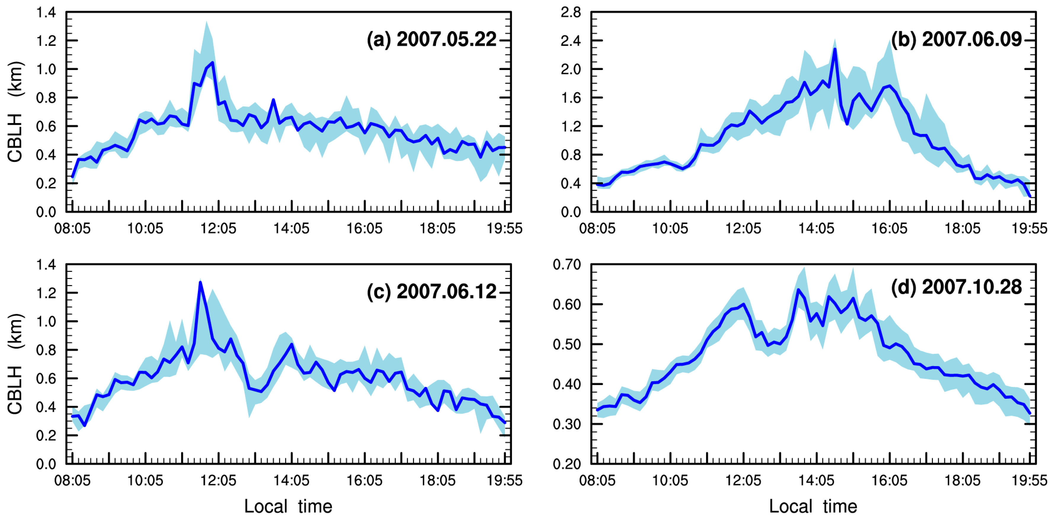
The CBLH values calculated at a time interval of 10 min via the parcel method based on profiles from the microwave radiometer are shown as purple solid lines in Figure 5a–d (the CBLH values are calculated every minute, then averaged every 11 min) and are also plotted as blue solid lines in Figure 6a–d. As mentioned earlier, the surface temperature measurement accuracy is 0.5 K, and the CBLH estimating through the parcel method relies on the surface temperature strongly. In order to evaluate the resulting CBLH with the varying surface temperature, increments from −0.5 K to 0.5 K are added to the surface temperature, which are then used to estimate the CBLH. The result is shown as Figure 6. It is easy to see that in the strong convective case (e.g., on 9 June 2007), wherein the maximum CBLH can reach to be more than 2.0 km, the uncertainties in the CBLH caused by the surface temperature are larger than that in the weak convective case (e.g., on 28 October 2007). Varying the surface temperature by 0.5 K results in differences of 0.2 km in the CBLH most times.
It is now clear that we can use the CCL to eliminate the cloud above the boundary layer top and thus find the CBLH below the CCL using lidar data (that is, only NRB values below the CCL are used to determine the CBLH). Using clear-sky data, the lidar methods are more likely to find a reliable CBLH estimate. Here, we use methods including the fitting, HM, MHM, and GM to calculate the CBLH with (or without) the CCL as an upper limiter. To compare the resulting CBLH with and without the CCL limiter added, we present Figure 7, Figure 8, Figure 9 and Figure 10.
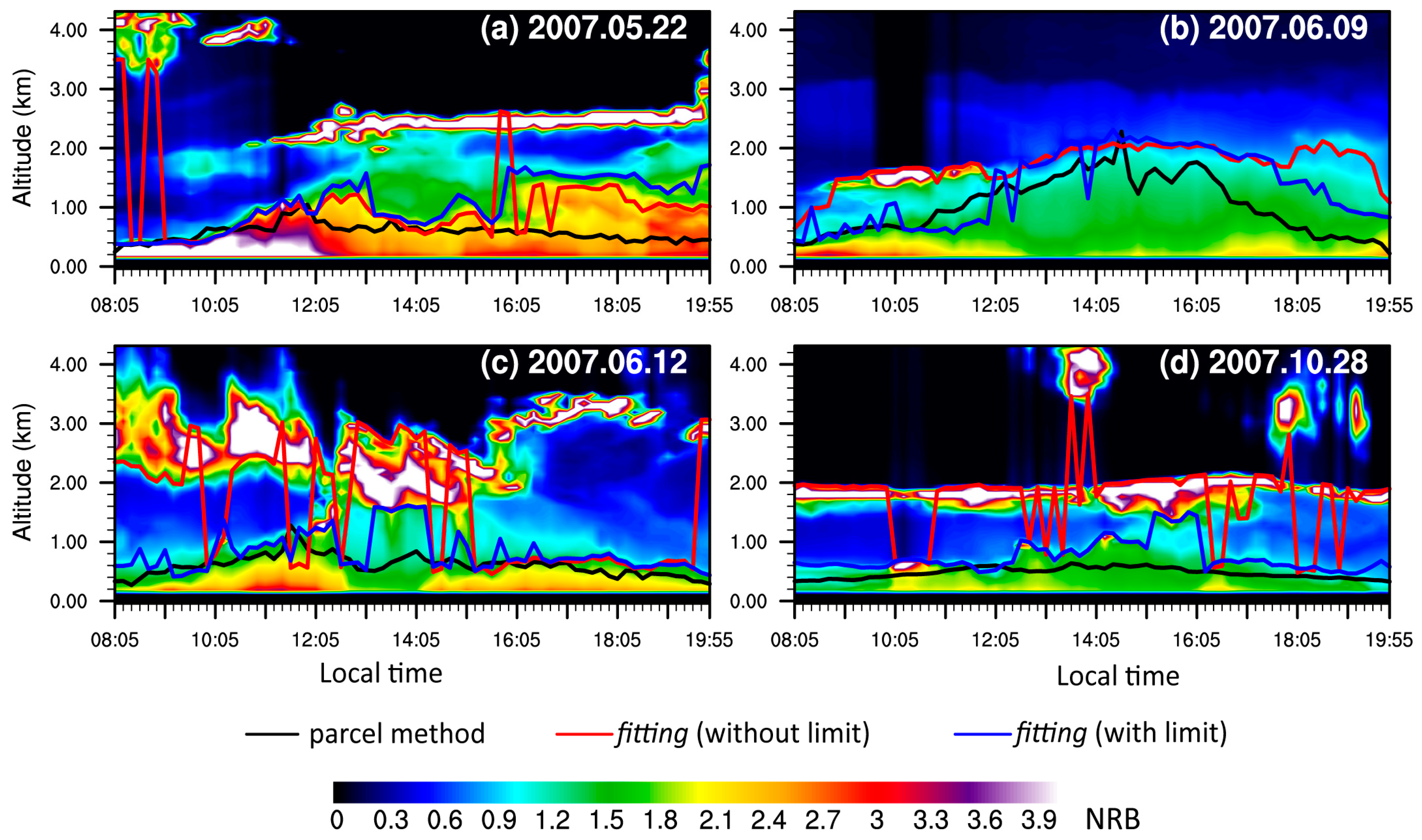
Figure 7 shows the CBLH values derived by the fitting with (or without) the calculated CCL as an upper limit. On 22 May 2007, the resulting CBL tops obtained from the fitting without the CCL limiter added are shown as red solid lines in Figure 7a. In cloudy periods (the white area between 08:05 and 11:15 above 3.2 km, as well as from 11:15 to 19:45, corresponding to the white area between 2.2 and 2.8 km), the calculated CBLH is close to the cloud top or cloud edges at certain times during the day (08:05, 08:15, 08:45, 08:55, 14:45 and 14:55) because of the strong backscatter caused by the clouds. The same phenomenon also occurs on the other three days. On 9 June 2007, clouds are present between 09:35 and 10:45 with a height of between 1.2 and 1.6 km, and the CBLH from fitting is also close to the height of the cloud top in cloudy periods. On 12 June and 28 October 2007, clouds are present almost all the time (the white areas between 1.5 and 3.5 km on June 12 and between 1.5 and 2 km on October 28), and the resulting CBLH values are still close to the cloud tops or in the clouds. Thus, although the fitting can tolerate more signal noise, the presence of clouds makes it difficult to capture the accurate CBLH at some times. As shown by the red lines in Figure 7, the resulting CBLH values without the CCL limiter added are certainly much higher than the CBLH values from the parcel method, and the diurnal variation in CBLH does not follow the typical daily CBLH variation well. However, the addition of the CCL limiter improves the results, causing the resulting CBLH to be closer to the CBLH estimated by the parcel method and to conform more the typical evolution of the CBLH, except for several times when the CBLH is not so well defined.
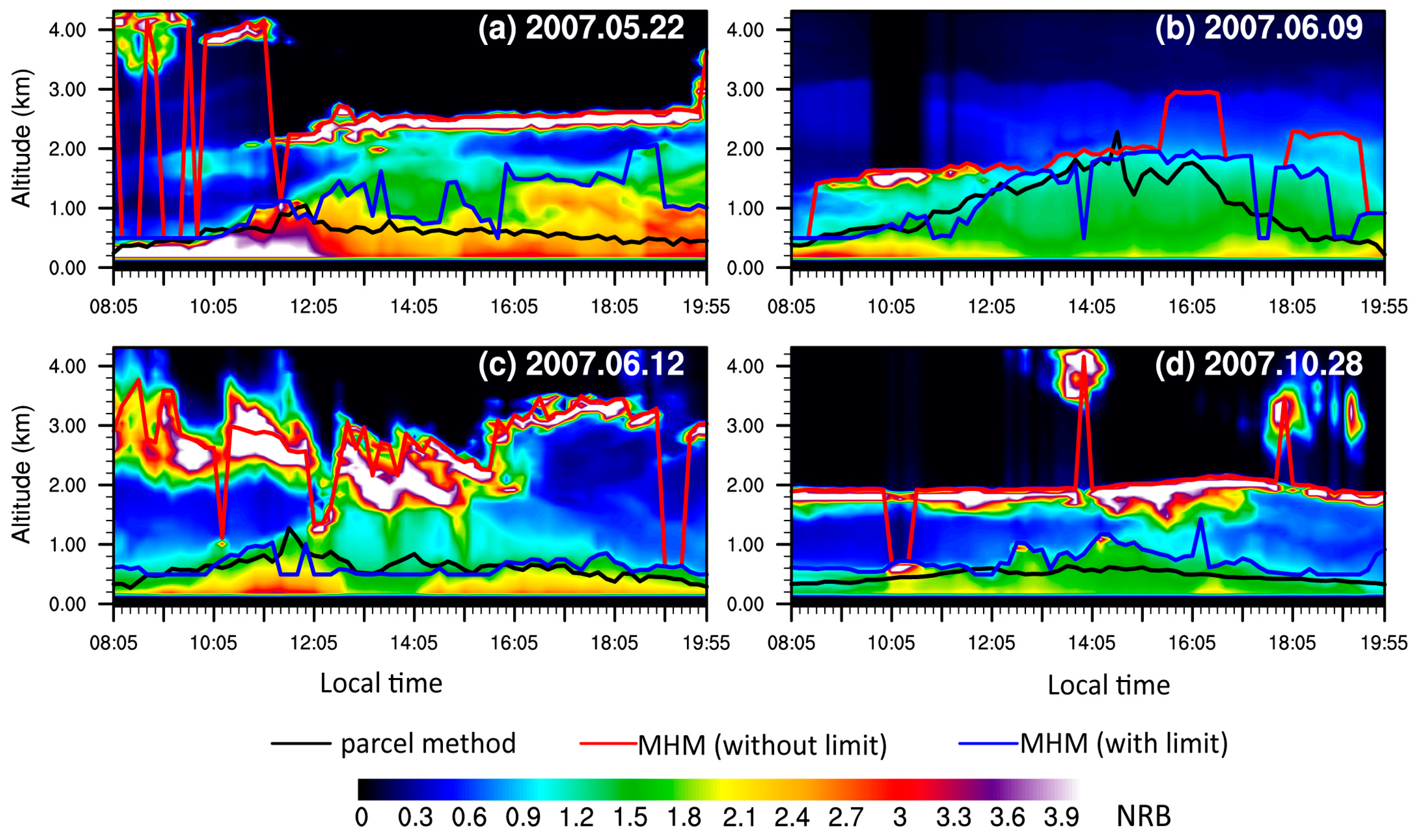
The results from the two wavelet methods with the CCL limiter added are similar and are shown as black lines in Figure 8 and Figure 9. We can see that the interference caused by clouds can be mostly eliminated for both methods. The resulting CBLH values generated by the two wavelet methods are closer to the CBLH values estimated by the parcel method. In addition, unreasonable lower CBLH estimates are obtained at several times (e.g., 11:55, 17:25, and 17:35 on 9 June 2007) with the CCL limiter added. This may be caused by high levels of NRB signal noise at those times so that the CBLH values were difficult to define. We believe the results could be improved by applying time continuity checks.
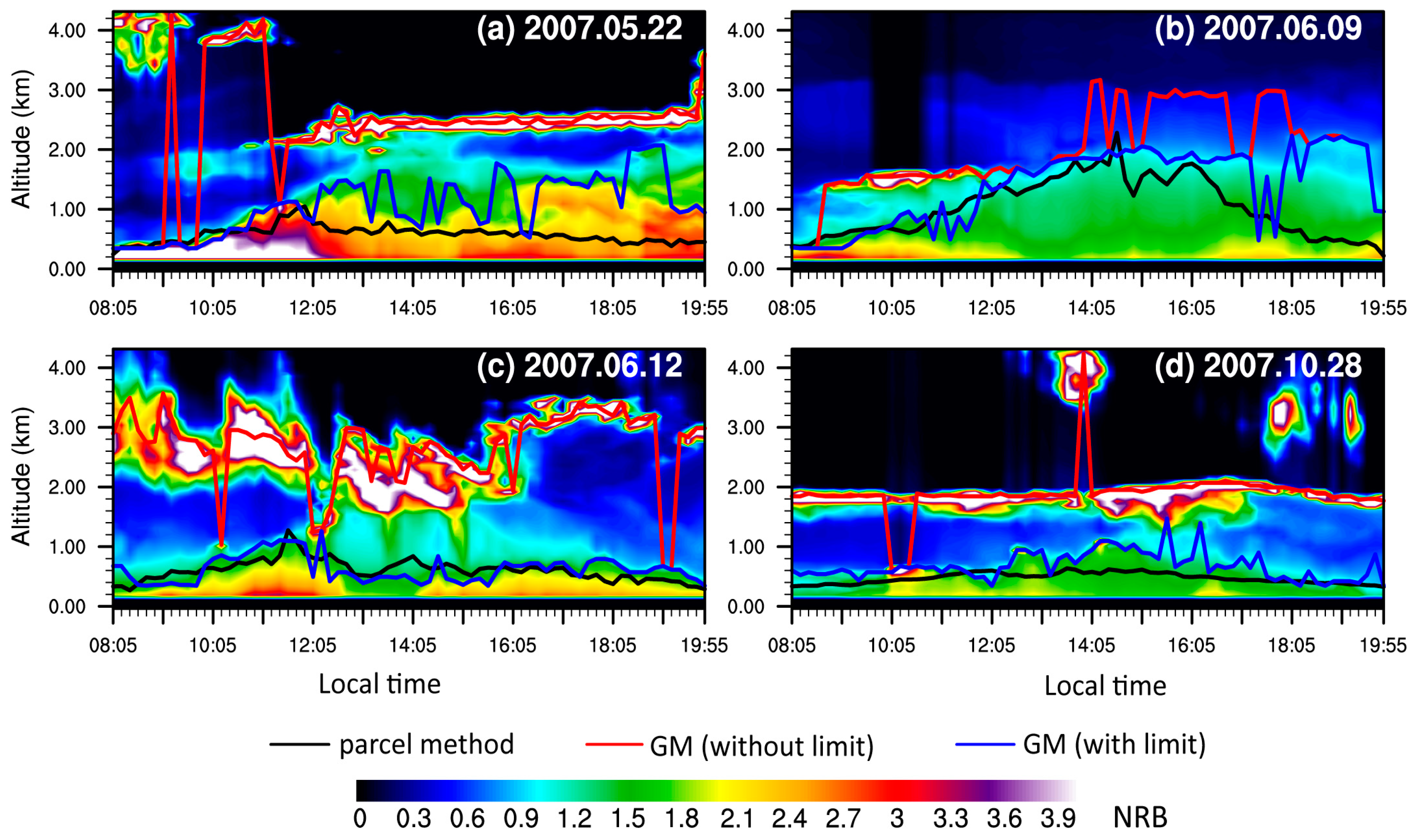
With the CCL limiter added, the estimated CBLH values from the GM are also improved (Figure 10), although the performance is less than the other three methods. Especially on 22 May and 9 June 2007, sudden changes in the CBLH occur, and thus the CBL tops do not follow the typical diurnal variation of the CBLH. This is understandable because the GM is more affected by the signal noise.
Except for good performance when clouds exist above the boundary layer, the four methods still yield a reliable CBLH when the boundary layer cloud occurs. From Figure 7, Figure 8, Figure 9 and Figure 10, for the period with boundary layer clouds (the white portion from 10:05 to 10:35 between 0.5 and 0.6 km on 28 October 2007), even when the CCL is not added as an upper limiter, the lidar methods are able to find the cloud top as the CBLH, which is reasonable. Fortunately, as we had hoped, the addition of the CCL limiter did not change the result.
Finally, for the four selected cloudy cases, the average biases between the resulting CBLHs with (or without) the limiter added and the CBLHs estimated by the parcel method for the four methods were calculated and are shown in Table 1. It is clear that the biases are smaller with than without the limiter added. However, the biases are still several hundred meters with the CCL limiter added. This is because, from afternoon to sunset, lower CBLH values are always obtained by the parcel method compared to the CBLH values derived from the lidar-base methods. This is understandable since the lidar-based methods always define the CBLH as the height with significant loss of signal somewhere in the entrainment zone, but the CBLH determined by the parcel method is the mixed layer top. In this way, for the boundary layer structure in the afternoon with a considerably deep entrainment zone, the CBLH from lidar data may be higher than that estimated by the parcel method.
5. Conclusions
Ground-based lidar data are widely used to calculate the convective boundary layer height (CBLH) over land because of their high temporal resolution. However, the retrieval process is influenced by clouds because of the high signal gradient they generate. Several studies have pointed out that the real CBLH sometimes differs from that derived by lidar methods in cloudy cases. In this study, four cases that include clouds above the boundary layer are used to evaluate the CBLH retrieval methods, and a new simple technique is proposed to obtain CBL tops under cloudy conditions. The technique aims at using the convective condensation level (CCL) as a limiter to limit the vertical extent of the lidar backscatter profile used by lidar methods to search for the boundary layer tops. More specifically, the CCL is regarded as a boundary that separates the boundary layer clouds from the clouds above the CBL, so only the signals below the CCL are used to determine the CBLH. The main advantage of using the CCL to estimate the lowest possible cloud base height of the cloud above the CBL is that the cloud base height is estimated based on knowledge of cloud formation. This is unlike the widely used threshold method, which is based on the lidar signal data and is more likely to be affected by the strong backscattered signals caused by aerosol layers aloft.
Analysis of the four lidar methods (the gradient method, the idealized backscatter method, and two forms of wavelet methods) applied to four cloudy cases reveals that unreasonable CBL tops are always obtained during cloudy periods, i.e., the cloud tops or a certain height in the cloud layers are more likely be interpreted as CBL tops. However, with the help of the convective condensation level (CCL) limiter, in terms of boundary layer clouds (i.e., clouds below the CCL), the clouds’ top is regarded as the CBL top for strong turbulence in clouds, and the methods either detect the top of a cloud or a point between clouds as the top of the CBL. For clouds above the CBL (i.e., clouds above the CCL), application of the CCL limiter results in more reasonable CBLH values.
Although the CCL limiter performs well in our cloudy cases, removing the interference from clouds above the boundary layer top to a certain extent, problems still remain that cannot be neglected. It is obvious that the CBL tops obtained using these methods do not follow the typical diurnal variation of the CBLH very well; that is, sudden changes in the CBLH can occur. At some times, the CBLH estimated by the lidar methods varies significantly from one ten-minute interval to the next. Such problems need to be resolved by further research; for example, by applying an algorithm to test the time-continuity of the retrieved CBLH.
Acknowledgments
We wish to thank the Semi-Arid Climate and Environment Observatory of Lanzhou University (SACOL) for providing the observational data. We also wish to acknowledge Qian Huang, Professor of the college of Atmospheric Sciences, Lanzhou University, for her help in offering theoretical guidance. Yi Yang was supported by the National Natural Science Foundation of China (No. 41375109) and the Arid Meteorology Science Foundation of the Institute of Arid Meteorology, China Meteorological Administration (No. IAM201513). Beidou Zhang was supported by the National Natural Science Foundation of China (No. 41305027).
Author Contributions
Yi Yang conceived the idea and designed the structure of this paper. Hong Li analyzed the data and wrote the paper. Xiao-Ming Hu proposed valuable comments on introduction and discussion parts. Zhongwei Huang, Guoyin Wang, and Beidou Zhang provided the data and gave proper advice on data processing.
Conflicts of Interest
The authors declare no conflict of interest.
References
- Stull, R.B. An Introduction to Boundary Layer Meteorology; Kluwer Academic Publishers: Dordrecht, The Netherlands, 1988; pp. 13–16. [Google Scholar]
- Holzworth, C.G. Estimates of mean maximum mixing depths in the contiguous United States. Mon. Weather Rev. 1964, 92, 235–242. [Google Scholar] [CrossRef]
- Menut, L.; Flamant, C.; Pelon, J.; Flamant, P.H. Urban boundary-layer height determination from lidar measurements over the Paris area. Appl. Opt. 1999, 38, 945–954. [Google Scholar] [CrossRef] [PubMed]
- Morille, Y.; Haeffelin, M.; Drobinski, P.; Pelon, J. STRAT: An automated algorithm to retrieve the vertical structure of the atmosphere from single-channel lidar data. J. Atmos. Ocean. Technol. 2007, 24, 761–775. [Google Scholar] [CrossRef]
- Granados-Muñoz, M.J.; Navas-Guzmán, F.; Bravo-Aranda, J.A.; Guerrero-Rascado, J.L.; Lyamani, H.; Fernández-Gálvez, J.; Alados-Arboledas, L. Automatic determination of the planetary boundary layer height using lidar: One-year analysis over southeastern Spain. J. Geophys. Res. 2012, 117, D18208. [Google Scholar] [CrossRef]
- Huang, M.; Gao, Z.; Miao, S.; Chen, F.; Lemone, M.A.; Li, J.; Hu, F.; Wang, L. Estimate of Boundary-Layer Depth over Beijing, China, Using Doppler Lidar Data during SURF-2015. Bound. Layer Meteorol. 2016, 162, 503–522. [Google Scholar] [CrossRef]
- Seibert, P.; Beyrich, F.; Gryning, S.-E.; Joffre, S.; Rasmussen, A.; Tercier, P. Review and intercomparison of operational methods for the determination of the mixing height. Atmos. Environ. 2000, 34, 1001–1027. [Google Scholar] [CrossRef]
- Lammert, A.; Bösenberg, J. Determination of the convective boundary-layer height with laser remote sensing. Bound. Layer Meteorol. 2006, 119, 159–170. [Google Scholar] [CrossRef]
- Sicard, M.; Pérez, C.; Rocadenbosch, F.; Baldasano, J.M.; García-Vizcaino, D. Mixed-layer depth determination in the barcelona coastal area from regular lidar measurements: methods, results and limitations. Bound. Layer Meteorol. 2006, 119, 135–157. [Google Scholar] [CrossRef]
- Emeis, S.; Schäfer, K.; Münkel, C. Surface-based remote sensing of the mixing-layer height—A review. Meteorol. Z. 2008, 17, 621–630. [Google Scholar] [CrossRef] [PubMed]
- Haeffelin, M.; Angelini, F.; Morille, Y.; Martucci, G.; Frey, S.; Gobbi, G.P.; Lolli, S.; O’Dowd, C.D.; Sauvage, L.; Xueref-Rémy, I.; et al. Evaluation of mixing-height retrievals from automatic profiling lidars and ceilometers in view of future integrated networks in Europe. Bound. Layer Meteorol. 2012, 143, 49–75. [Google Scholar] [CrossRef]
- Pappalardo, G.; Amodeo, A.; Apituley, A.; Comeron, A.; Freudenthaler, V.; Linné, H.; Ansmann, A.; Bösenberg, J.; D’Amico, G.; Mattis, I.; et al. EARLINET: Towards an advanced sustainable European aerosol lidar network. Atmos. Meas. Tech. 2014, 7, 2929–2980. [Google Scholar] [CrossRef]
- Atsushi, S.; Nobuo, S.; Ichiro, M.; Kimio, A.; Itsushi, U.; Toshiyuki, M.; Naoki, K.; Kazuma, A.; Akihiro, U.; Akihiro, Y. Continuous observations of Asian dust and other aerosols by polarization lidars in China and Japan during ACE-Asia. J. Geophys. Res. 2004, 109, 1255–1263. [Google Scholar]
- Guerrero-Rascado, J.L.; Landulfo, E.; Antuña, J.C.; Barbosa, H.M.J.; Barja, B.; Bastidas, Á.E.; Bedoya, A.E.; Costa, R.; Estevan, R.; Forno, R.; et al. Latin American Lidar Network (LALINET) for aerosol research: Diagnosis on network instrumentation. J. Atmos. Sol. Terr. Phys. 2016, 138–139, 112–120. [Google Scholar] [CrossRef]
- Welton, E.J.; Campbell, J.R.; Spinhirne, J.D.; Scott, V.S. Global monitoring of clouds and aerosols using a network of micropulse lidar systems. Proc. Int. Soc. Opt. Eng. 2001, 4153, 151–158. [Google Scholar]
- Baars, H.; Ansmann, A.; Engelmann, R.; Althausen, D. Continuous monitoring of the boundary-layer top with lidar. Atmos. Chem. Phys. 2008, 8, 7281–7296. [Google Scholar] [CrossRef]
- Pal, S.; Behrendt, A.; Wulfmeyer, V. Elastic-backscatter-lidar-based characterization of the convective boundary layer and investigation of related statistics. Ann. Geophys. 2010, 28, 825–847. [Google Scholar] [CrossRef]
- Hayden, K.L.; Anlauf, K.J.; Hoff, R.M.; Strapp, J.W.; Bottenheim, J.W.; Wiebe, H.A.; Froude, F.A.; Martin, J.B.; Steyn, D.G.; McKendry, I.G. The vertical chemical and meteorological structure of the boundary layer in the Lower Fraser Valley during Pacific’93. Atmos. Environ. 1997, 31, 2089–2105. [Google Scholar] [CrossRef]
- Flamant, C.; Pelon, J.; Flamant, P.H.; Durand, P. Lidar determination of the entrainment zone thickness at the top of the unstable marine atmospheric boundary layer. Bound. Layer Meteorol. 1997, 83, 247–284. [Google Scholar] [CrossRef]
- Steyn, D.G.; Baldi, M.; Hoff, R.M. The detection of mixed layer depth and entrainment zone thickness from lidar backscatter profiles. J. Atmos. Ocean. Technol. 1999, 16, 953–959. [Google Scholar] [CrossRef]
- Davis, K.J.; Gamage, N.; Hagelberg, C.R.; Kiemle, C.; Lenschow, D.H.; Sullivan, P.P. An objective method for deriving atmospheric structure from airborne lidar observations. J. Atmos. Ocean. Technol. 2000, 17, 1455–1468. [Google Scholar] [CrossRef]
- Cohn, S.A.; Angevine, W.M. Boundary layer height and entrainment zone thickness measured by lidars and wind-profiling radars. J. Appl. Meteorol. 2000, 39, 1233–1247. [Google Scholar] [CrossRef]
- Brooks, I.M. Finding boundary layer top: Application of a wavelet covariance transform to lidar backscatter profiles. J. Atmos. Ocean. Technol. 2003, 20, 1092–1105. [Google Scholar] [CrossRef]
- Pal, S.; Haeffelin, M.; Batchvarova, E. Exploring a geophysical process-based attribution technique for the determination of the atmospheric boundary layer depth using aerosol lidar and near-surface meteorological measurements. J. Geophys. Res. Atmos. 2013, 118, 9277–9295. [Google Scholar] [CrossRef]
- Bravo-Aranda, J.A.; Moreira, G.A.; Navas-Guzmán, F.; Granados-Muñoz, M.J.; Guerrero-Rascado, J.L.; Pozo-Vázquez, D.; Arbizu-Barrena, C.; Reyes, F.J.O.; Mallet, M.; Alados-Arboledas, L. PBL height estimation based on lidar depolarisation measurements (POLARIS). Atmos. Chem. Phys. Discuss. 2016, 1–24. [Google Scholar] [CrossRef]
- Li, H.; Yang, Y.; Hu, X.M.; Huang, Z.W.; Wang, G.Y.; Zhang, B.D.; Zhang, T.J. Evaluation of retrieval methods of daytime convective boundary layer height based on lidar data. J. Geophys. Res. 2017. [Google Scholar] [CrossRef]
- Hennemuth, B.; Lammert, A. Determination of the atmospheric boundary layer height from radiosonde and lidar backscatter. Bound. Layer Meteorol. 2006, 120, 181–200. [Google Scholar] [CrossRef]
- Grimsdell, A.W.; Angevine, W.M. Convective boundary layer height measurement with wind profilers and comparison to cloud base. J. Atmos. Ocean. Technol. 1998, 15, 1331–1338. [Google Scholar] [CrossRef]
- Collaud-Coen, M.; Praz, C.; Haefele, A.; Ruffieux, D.; Kaufmann, P.; Calpini, B. Determination and climatology of the planetary boundary layer height above the swiss plateau by in situ and remote sensing measurements as well as by the COSMO-2 model. Atmos. Chem. Phys. 2014, 14, 13205–13221. [Google Scholar] [CrossRef]
- Angevine, W.M.; White, A.B.; Avery, S.K. Boundary-layer depth and entrainment zone characterization with a boundary-layer profiler. Bound. Layer Meteorol. 1994, 68, 375–385. [Google Scholar] [CrossRef]
- McGrath-Spangler, E.L.; Denning, A.S. Estimates of North American summertime planetary boundary layer depths derived from space-borne lidar. J. Geophys. Res. 2012, 117, D15101. [Google Scholar] [CrossRef]
- Wang, Z.; Sassen, K. Cloud type and macrophysical property retrieval using multiple remote sensors. J. Appl. Meteorol. 2001, 40, 1665–1683. [Google Scholar] [CrossRef]
- Winker, D.M.; Vaughan, M.A. Vertical distribution of clouds over Hampton, Virginia, observed by lidar under the ECLIPS and FIRE ETO programs. Atmos. Res. 1994, 34, 117–133. [Google Scholar] [CrossRef]
- Caicedo, V.; Rappenglueck, B.; Lefer, B.; Morris, G.; Toledo, D.; Delgado, R. Comparison of aerosol lidar retrieval methods for boundary layer height detection using ceilometer backscatter data. Atmos. Meas. Tech. Discuss. 2016, 1–24. [Google Scholar] [CrossRef]
- Huang, Z.; Huang, J.; Bi, J.; Wang, G.; Wang, W.; Fu, Q.; Li, Z.; Tsay, S.-C.; Shi, J. Dust aerosol vertical structure measurements using three MPL lidars during 2008 China-U.S. joint dust field experiment. J. Geophys. Res. 2010, 115, 1307–1314. [Google Scholar] [CrossRef]
- Campbell, J.R.; Hlavka, D.L.; Welton, E.J.; Flynn, C.J.; Turner, D.D.; Spinhirne, J.D.; Scott, V.S.; Wang, I.H. Full-Time, Eye-Safe Cloud and Aerosol Lidar Observation at Atmospheric Radiation Measurement Program Sites: Instruments and Data Processing. J. Atmos. Ocean. Technol. 2002, 19, 431–442. [Google Scholar] [CrossRef]
- Sasano, Y.; Shimizu, H.; Takeuchi, N.; Okuda, M. Geometrical form factor in the laser radar equation: An experimental determination. Appl. Opt. 1979, 18, 3908–3910. [Google Scholar] [CrossRef] [PubMed]
- Dho, S.W.; Park, Y.J.; Kong, H.J. Experimental determination of a geometric form factor in a lidar equation for an inhomogeneous atmosphere. Appl. Opt. 1997, 36, 6009–6010. [Google Scholar] [CrossRef] [PubMed]
- Wandinger, U.; Ansmann, A. Experimental determination of the lidar overlap profile with raman lidar. Appl. Opt. 2002, 41, 511–514. [Google Scholar] [CrossRef] [PubMed]
- Mao, F.; Gong, W.; Li, J. Geometrical form factor calculation using monte carlo integration for lidar. Opt. Laser Technol. 2012, 44, 907–912. [Google Scholar] [CrossRef]
- Chen, R.; Jiang, Y.; Wang, H. Calculation method of the overlap factor and its enhancement for airborne lidar. Opt. Commun. 2014, 331, 181–188. [Google Scholar] [CrossRef]
- Fernald, F.G.; Herman, B.M.; Reagan, J.A. Determination of Aerosol Height Distributions by Lidar. J. Appl. Meteorol. 1972, 11, 482–489. [Google Scholar] [CrossRef]
- Ware, R.; Carpenter, R.; Güldner, J.; Liljegren, J.; Nehrkorn, T.; Solheim, F.; Vandenberghe, F. A multichannel radiometric profiler of temperature, humidity, and cloud liquid. Radio Sci. 2003, 44, 77–88. [Google Scholar] [CrossRef]
- Ruffieux, D.; Nash, J.; Jeannet, P.; Agnew, J.L. The COST 720 temperature, humidity, and cloud profiling campaign: TUC. Meteorol. Z. 2006, 15, 5–10. [Google Scholar] [CrossRef]
- Eresmaa, N.; Karppinen, A.; Joffre, S.M.; Räsänen, J.; Talvitie, H. Mixing height determination by ceilometers. Atmos. Chem. Phys. 2006, 6, 1485–1493. [Google Scholar] [CrossRef]
- Zhang, B.D.; Huang, J.P.; Guo, Y.; Shang, J.; Wu, Q. Retrieval of atmospheric temperature, humidity profile and attenuation estimation using a twele channel ground-based microwave radiometer. J. Lanzhou Univ. (Nat. Sci.) 2015, 2, 193–201. (In Chinese) [Google Scholar]
- Wang, Z.; Cao, X.; Zhang, L.; Notholt, J.; Zhou, B.; Liu, R.; Zhang, B. Lidar measurement of planetary boundary layer height and comparison with microwave profiling radiometer observation. Atmos. Meas. Tech. 2012, 5, 1965–1972. [Google Scholar] [CrossRef]
- Di-Liberto, L.; Angelini, F.; Pietroni, I.; Cairo, F.; Di Donfrancesco, G.; Viola, A.; Argentini, S.; Fierli, F.; Gobbi, G.; Maturilli, M.; et al. Estimate of the arctic convective boundary layer height from lidar observations: a case study. Adv. Meteorol. 2012, 8, 978–988. [Google Scholar] [CrossRef]
- Eresmaa, N.; Härkönen, J.; Joffre, S.M.; Schultz, D.M.; Karppinen, A.; Kukkonen, J. A Three-Step Method for Estimating the Mixing Height Using Ceilometer Data from the Helsinki Testbed. J. Appl. Meteor. Climatol. 2012, 51, 2172–2187. [Google Scholar] [CrossRef]
- Davis, K.J.; Lenschow, D.H.; Oncley, S.P.; Kiemle, C.; Ehret, G.; Giez, A. Role of entrainment in surface-atmosphere interactions over the boreal forest. J. Geophys Res. 1997, 102, 29219–29230. [Google Scholar] [CrossRef]
- Zhou, Z.; Adeli, H. Time-frequency signal analysis of earthquake records using Mexican hat wavelets. Comput. Aided Civ. Inf. 2003, 18, 379–389. [Google Scholar] [CrossRef]
- Rogers, R.; Yau, M. A Short Course in Cloud Physics, 3nd ed.; Pergamon Press: New York, NY, USA, 1989. [Google Scholar]
- Stackpole, J.D. Numerical analysis of atmospheric soundings. J. Appl. Meteorol. 1967, 6, 464–467. [Google Scholar] [CrossRef]
- Stull, R.B. Meteorology Today: For Scientist and Engineers; West Publishing Company: Minneapolis, MN, USA, 1995; p. 385. [Google Scholar]
Figure 1.
(a) Normalized Relative Backscatter (NRB) profile at 13:00 local time on July 23, 2007 and profiles of (b) fitted curve (); (c) Haar wavelet coefficient (HM ); (d) gradient (); and (e) Mexican hat wavelet coefficient (MHM ). The CBL (Convective Boundary Layer) tops from these profiles are shown as horizontal lines, and the parameter used by the HM and MHM is set to 300 m.

Figure 2.
Clear-sky case. (a) NRB profile at 13:00 local time on 23 July 2007 and (b) Haar wavelet coefficients matrix with varying wavelet dilation; (c) signal gradient profile () and (d) Mexican hat wavelet coefficients matrix with varying wavelet dilation; Dots in (b,d) indicate altitudes at which the wavelet coefficient maxima occur under different wavelet dilations. Horizontal dotted line in (a) (or (c)) indicates average altitude where the Haar (or Mexican hat) wavelet coefficient is at a maximum.
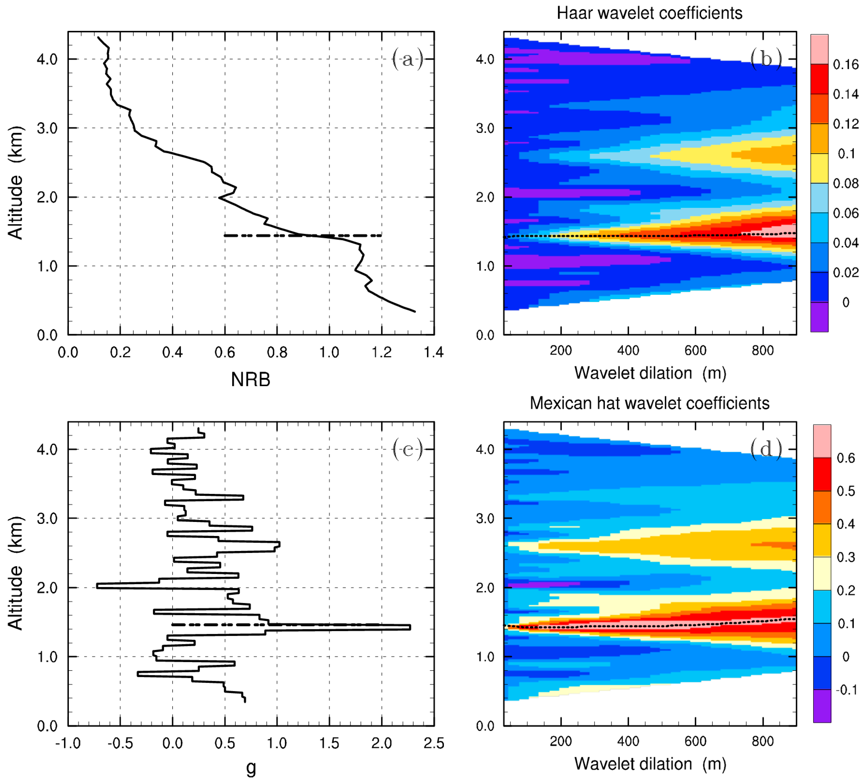
Figure 3.
Cloudy case. (a) NRB profile at 09:00 local time on 23 June 2007 and (b) Haar wavelet coefficient matrix with varying wavelet dilation; (c) signal gradient profile () and (d) Mexican hat wavelet coefficients matrix with varying wavelet dilation; Dots in (b) and (d) indicate altitudes at which the wavelet coefficient maxima occur under different wavelet dilations. Horizontal dotted line in (a) (or (c)) indicates average altitude where the Haar (or Mexican hat) wavelet coefficient is at a maximum.


Figure 4.
Convective boundary layer height (CBLH) determined by the parcel method applied to the microwave radiometer profile. The profile is measured at 13:00 local time on 23 July 2007 at SACOL (the Semi-arid Climate Observatory and Laboratory of Lanzhou University).
Figure 4.
Convective boundary layer height (CBLH) determined by the parcel method applied to the microwave radiometer profile. The profile is measured at 13:00 local time on 23 July 2007 at SACOL (the Semi-arid Climate Observatory and Laboratory of Lanzhou University).

Figure 5.
Time–height diagram of NRB (averaged every 11 min) on (a) 22 May; (b) 9 June; (c) 12 June; and (d) 28 October 2007. The calculated lifting condensation level (LCL) and convective condensation level (CCL) are marked by red solid lines and black solid lines, respectively. The CBLH calculated by the parcel method is marked by purple solid lines.
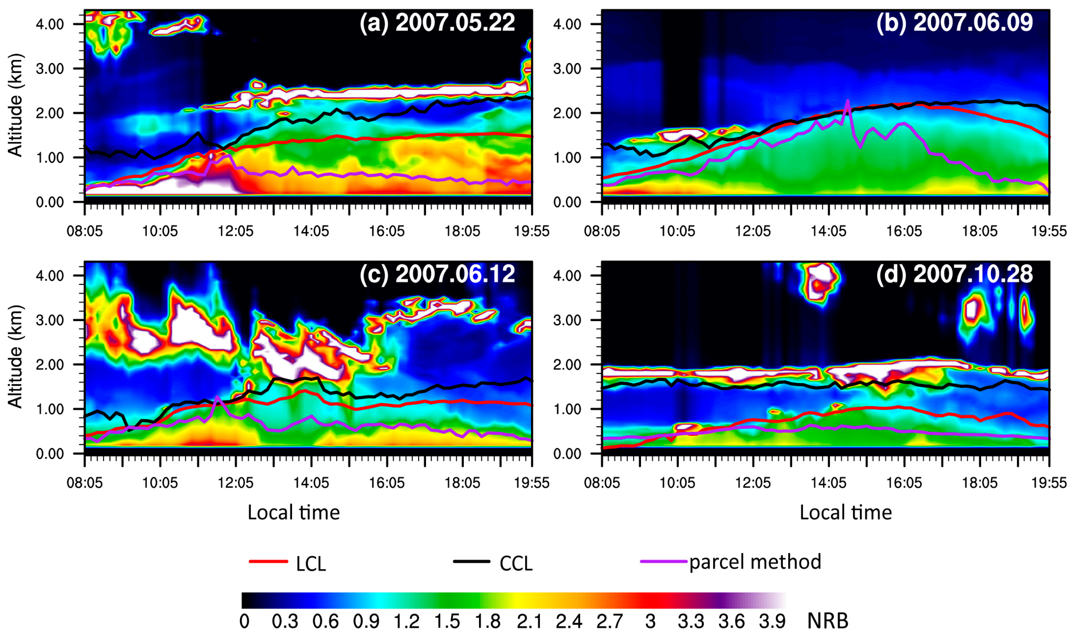
Figure 6.
The CBLH values calculated by the parcel method on (a) 22 May; (b) 9 June; (c) 12 June; and (d) 28 October 2007 (blue solid lines). The shaded area in light blue in each plot represents the uncertainties in the CBLH caused by the surface temperature.
Figure 6.
The CBLH values calculated by the parcel method on (a) 22 May; (b) 9 June; (c) 12 June; and (d) 28 October 2007 (blue solid lines). The shaded area in light blue in each plot represents the uncertainties in the CBLH caused by the surface temperature.

Figure 7.
Time–height diagram of NRB (averaged every 11 min) on (a) 22 May; (b) 9 June; (c) 12 June; and (d) 28 October 2007. The CBLH calculated by the idealized backscatter method (fitting) with (or without) the calculated CCL as an upper limit is marked by blue solid lines (or red solid lines). The CBLH estimated by the parcel method is marked by black solid lines.

Figure 8.
Time–height diagram of NRB (averaged every 11 minutes) on (a) 22 May; (b) 9 June; (c) 12 June; and (d) 28 October 2007. The CBLH calculated by the Haar wavelet method (HM) with (or without) the calculated CCL as an upper limit is marked by blue solid lines (or red solid lines), and the used by the HM is set to 300 m based on the previous sensitivity test. The CBLH estimated by the parcel method is marked by black solid lines.
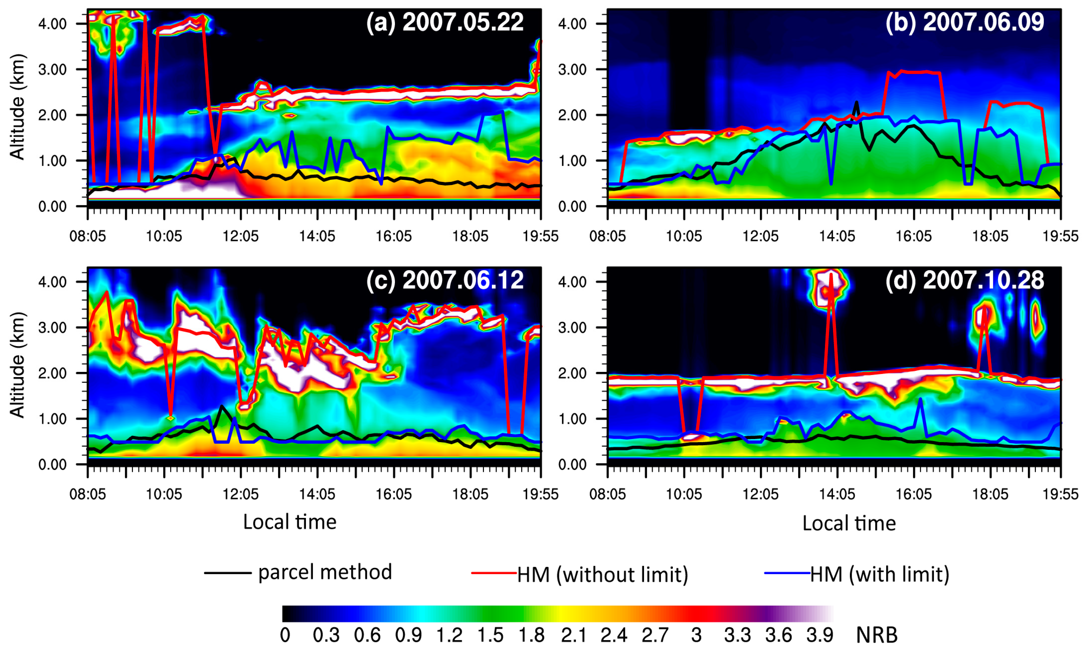
Figure 9.
Time–height diagram of NRB (averaged every 11 min) on (a) 22 May; (b) 9 June; (c) 12 June; and (d) 28 October 2007. The CBLH calculated by the Mexican hat wavelet method (MHM) with (or without) the calculated CCL as an upper limit is marked by blue solid lines (or red solid lines), and the used by the HM is set to 300 m based on the previous sensitivity test. The CBLH estimated by the parcel method is marked by black solid lines.

Figure 10.
Time–height diagram of NRB (averaged every 11 min) on (a) 22 May; (b) 9 June; (c) 12 June; and (d) 28 October 2007. The CBLH calculated by the gradient method (GM) with (or without) the calculated CCL as an upper limit is marked by blue solid lines (or red solid lines). The CBLH estimated by the parcel method is marked by black solid lines.

Table 1.
Average biases between the resulting CBLHs (Convective Boundary Layer Heights) with (or without) the limiter added and the CBLHs estimated by the parcel method for the four methods on four different days (km).
Table 1.
Average biases between the resulting CBLHs (Convective Boundary Layer Heights) with (or without) the limiter added and the CBLHs estimated by the parcel method for the four methods on four different days (km).
| Date (Year/Month/Day) | GM (Without Limit) | GM (With Limit) | fitting (Without Limit) | fitting (With Limit) | HM (Without Limit) | HM (With Limit) | MHM (Without Limit) | MHM (With Limit) |
|---|---|---|---|---|---|---|---|---|
| 2007.05.22 | 1.796 | 0.532 | 0.530 | 0.507 | 1.949 | 0.522 | 2.001 | 0.513 |
| 2007.06.09 | 0.953 | 0.485 | 0.712 | 0.436 | 0.822 | 0.350 | 0.796 | 0.348 |
| 2007.06.12 | 2.092 | 0.180 | 1.046 | 0.271 | 2.144 | 0.174 | 2.149 | 0.173 |
| 2007.10.28 | 1.412 | 0.222 | 1.263 | 0.279 | 1.480 | 0.243 | 1.494 | 0.244 |
fitting: the idealized backscatter method; GM: the gradient method; HM: the Haar wavelet method; MHM: the Mexican hat wavelet method.
© 2017 by the authors. Licensee MDPI, Basel, Switzerland. This article is an open access article distributed under the terms and conditions of the Creative Commons Attribution (CC BY) license (http://creativecommons.org/licenses/by/4.0/).
Share and Cite
MDPI and ACS Style
Li, H.; Yang, Y.; Hu, X.-M.; Huang, Z.; Wang, G.; Zhang, B. Application of Convective Condensation Level Limiter in Convective Boundary Layer Height Retrieval Based on Lidar Data. Atmosphere 2017, 8, 79. https://doi.org/10.3390/atmos8040079
AMA Style
Li H, Yang Y, Hu X-M, Huang Z, Wang G, Zhang B. Application of Convective Condensation Level Limiter in Convective Boundary Layer Height Retrieval Based on Lidar Data. Atmosphere. 2017; 8(4):79. https://doi.org/10.3390/atmos8040079
Chicago/Turabian StyleLi, Hong, Yi Yang, Xiao-Ming Hu, Zhongwei Huang, Guoyin Wang, and Beidou Zhang. 2017. "Application of Convective Condensation Level Limiter in Convective Boundary Layer Height Retrieval Based on Lidar Data" Atmosphere 8, no. 4: 79. https://doi.org/10.3390/atmos8040079
Note that from the first issue of 2016, this journal uses article numbers instead of page numbers. See further details here.