Article

Variations of Carbon Monoxide Concentrations in the Megacity of São Paulo from 2000 to 2015 in Different Time Scales

by
José Roberto Rozante
1,*,
Vinícius Rozante
2,
Débora Souza Alvim
1,
Antônio Ocimar Manzi
1,
Júlio Barboza Chiquetto
3,
Monica Tais Siqueira D’Amelio
4 and
Demerval Soares Moreira
5
1
Center for Weather Forecasting and Climate Studies (CPTEC), National Institute for Space Research (INPE), Cachoeira Paulista SP 12630-000, Brazil
2
School of Chemical Engineering (FEQ), State University of Campinas (UNICAMP), Campinas SP 13083-970, Brazil
3
Department of Geography, University of Sao Paulo (USP), São Paulo SP 05508-000, Brazil
4
Research Group on Environment and Sustainability (GPMAS), University of São Francisco (USF), Itatiba SP 13251-900, Brazil
5
São Paulo State University (UNESP), School of Sciences, Bauru SP 17033-360, Brazil
*
Author to whom correspondence should be addressed.
Atmosphere 2017, 8(5), 81; https://doi.org/10.3390/atmos8050081
Submission received: 13 March 2017 / Revised: 17 April 2017 / Accepted: 20 April 2017 / Published: 28 April 2017
(This article belongs to the Special Issue Urban Air Pollution)

Abstract

:
Air pollution is an important public health issue. High levels of carbon monoxide in the atmosphere are hazardous to human health. Studies regarding the concentration of this and other gases in the atmosphere allow political actions to manage and reduce the emission of pollutants. In this context, this paper studied the annual, seasonal, weekly and daily variations of carbon monoxide (CO) concentration for the Metropolitan Region of São Paulo (MRSP). We studied three sites in the MRSP, two of them are located in areas under the influence of heavy vehicle traffic (Osasco and Congonhas) and the third one in a city park (Ibirapuera Park). The results showed high influence of gasoline vehicles on CO emission. In the annual scale, CO concentration decreased due to improvements in emission technology, despite the increasing number of vehicles. CO emission showed a seasonal, weekly and diurnal cycle associated to meteorological conditions and emission patterns. The highest values of mean concentration were observed in June/July for Osasco (2.20 ppm), Congonhas (2.04 ppm) and Ibirapuera (1.04 ppm), during the morning, due to weak dispersion of the polluting gases and higher emission from the rush hours.

1. Introduction

Urban atmospheric pollution has increased due to an increment in automobiles and industrial emissions, which worsen air quality and promote hazardous conditions for people, plants and animal life. The Metropolitan Region of São Paulo (MRSP), with 21 million of habitants and 39 cities, including the capital São Paulo with 11 million inhabitants, is the sixth largest human conglomeration in the word [1]. According to the Environmental Agency of the State of São Paulo (CETESB), about 97% of Carbon Monoxide (CO) concentrations are originated by vehicle emissions [2].
CO is a colorless, tasteless and odorless gas, flammable and dangerous to human health due to its toxicity and for promoting chemical asphyxiation. The main CO sources are combustion processes related to energy, heating, vehicle transport, biomass burning, the oxidation of methane and volatile organic compounds (VOCs). Its natural sources are volcanic activity, electrical discharge and natural gas emissions. CO is produced by chemical reactions in the atmosphere between the hydroxyl radical (OH) and methane (CH4) and other hydrocarbons (HC), besides reactions between alkenes and ozone (O3), and reactions from isoprene and terpenes with OH and O3 [3,4]. The major sink of CO is its reaction with OH, while dry deposition and stratospheric flux are considered minor sinks [5,6,7]. At the troposphere, the hydroxyl free radical (OH) oxidizes carbon monoxide (CO) producing hydroperoxide radicals (HO2) [8]:
CO + OH → CO2 + H
H + O2 + M → HO2 + M
According to [9], excess NOx (NOx = NO + NO2), as in the Megacity of São Paulo atmosphere with a NO mixing ratio higher than 10 pptv, promote O3 production following reactions (1) and (2). Otherwise, O3 is destroyed by hydroperoxylate radical. However, any chain reaction dissipates CO, producing carbon dioxide. Reaction (1) is a fast reaction, independent of temperature [10]. It implies a CO global lifetime of two months and is the most significant OH sink in the troposphere [9,11,12]. In the atmosphere, the main CO source is the methane oxidation by OH, which produces formaldehyde (CH2O) and then carbon monoxide. This reaction, together with the (1) reaction, consume most of the OH in the troposphere. For this reason, CO and CH4 tropospheric concentrations are very important indicators of the tropospheric oxidizing capacity, represented specifically by ozone and hydroxyl radical concentrations. CO is not considered a greenhouse gas because it does not have the capacity to absorb infrared radiation. The atmospheric CO balance shows the destruction of methane and the production of CO2, O3 and sulfate aerosols, which might affect the climate. These reactions modify the balance CO-CH4, affecting water and temperature [13]. The bi-directional interaction between chemistry and the climate over CO is evident. From the industrial revolution to the 1980 decade, global CO concentration presented a marked increase; however, since 1980, this concentration has decreased [14,15], probably due the use of catalytic converters in cars [7]. Studies suggest that a decrease on global CO concentration would increase the OH radical, and consequently, the sink rate of CH4. This would modify the oxidizing capacity of the troposphere [9,11,16,17]. As a policy measure to reduce the atmospheric loading of CH4, a 50% reduction in the industrial emissions to 250 Tg-CO yr−1 would cause an increase by about 3.5% in OH concentrations leading to enhanced photochemical loss of CH4. The photochemical production of CO, although quite uncertain, may account for 40–50% of the total CO source. According to three-dimensional global model calculations, CH4 oxidation produces 700 Tg-CO yr−1. Photochemical production of CO from the oxidation of naturally emitted NMHC is calculated to be equal to about 450 Tg-CO yr−1, close to one third of the total photochemical source of CO. Anthropogenic NMHC oxidation forms 110 Tg-CO yr−1 [18].
Both macro and micro-meteorological factors play a role in the rate of dispersion of the ambient CO emitted. The fundamental meteorological factors involved are wind speed, wind direction, turbulence, and atmospheric stability. These factors are, of course, important for transport and diffusion of all air pollutants. In the case of CO levels in city streets, where people are located very close to the sources, the micro-meteorological factors become very important. This is due to the physical characteristics of cities (tall buildings and other obstacles such as autos) which often have a profound effect on the generation and characteristics of small scale turbulence and diffusion. Since autos usually are moving, they create their own small albeit intense field of vehicle-induced mechanical turbulence. The diffusion resulting from there is very important in the determination of nearby CO concentrations. This effect is intensified when the wind speed is very low (mean wind speed of <1.3 m s−1). When the wind speed is high, the air flowing over and around buildings will create additional turbulence and mixing which will be superimposed upon that generated by vehicles. This phenomenon also accounts for the fact that lower concentrations are expected with higher wind speeds. The development of turbulence depends upon the general stability of the atmosphere [19].
The concentration of CO in the vicinity of a city street is the product of emissions not only on that street but also from more distant up-wind streets. Very approximately, the “background” concentration from more distant sources will depend upon the number of emitting streets upwind and macro-meteorological factors, the depth through which effective mixing occurs and the wind speed through that depth. Mixing depth and wind speed determine the effective rate at which “fresh air” (or at least, less polluted) is transported into the city [19].
High CO concentration is considered very toxic to humans because it can cause acute intoxication, leaving sequels or promoting death by asphyxiation. The interaction of hemoglobin with CO is 240 times greater than with oxygen (O2), so, carboxyhemoglobin is formed instead of oxyhemoglobin [20]. When the atmosphere is rich in CO, O2 has difficulty to reach the tissue, causing death by suffocation. The acute affects of CO poisoning are well understood. Generally, in otherwise healthy people, headache develops when COHb concentrations reach 10%; tinnitus (ringing in the ear) and lightheadedness at 20%; nausea, vomiting, and weakness at 20–30%; clouding of consciousness and coma at around 35%; and death at around 50%. However, the outcomes of long-term, low-concentration CO exposures are less well understood. Because of the critical nature of blood flow and O2 delivery to the heart and brain, these organ, as well as the lungs (the first organ to come into contact with the pollutant), have received the most attention [21,22]. It was demonstrated statistically that maternal exposure to air pollution in the first trimester of gestation may contribute to lower fetal weight gain. Although it is difficult to isolate the influence of each pollutant, it was possible to show the greater influence of CO on newborn weight. Due to these and other factors, the monitoring and prevention of this gas is extremely important [23], even if it does not exceed the air quality standards in the MRSP.
During the Olympic Games in Atlanta, USA, a series of measurements were implemented in order to reduce urban pollution. During the three weeks of the games, traffic decreased by around 22%. There was a reduction in the daily peak levels of O3 (28%), NO2 (7%), CO (19%) and Particulate Matter (MP10) (16%) compared to the three weeks before and after the games. In that period, there was a 40% decrease in children asthma consultations and a decline of 11–19% in asthma care at all ages in emergency services in the city. During the Beijing Olympics, there was a decrease in PM2.5 from 78.8 μg m−3 to 46.7 μg m−3, and in O3 concentrations, from 65.8 ppb to 61 ppb and a decrease of 41.6% in asthma treatment in emergency services [24,25].
In Munich, Germany, 2860 children were monitored from their birth up to 4 years of age, and another 3061, up to 6 years of age, to study pollution effects on their health. The authors categorized the distance of children’s houses to major traffic routes in: less than 50 m, 50–250 m, 250–1000 m, and >1000 m. The study showed significant inverse associations between the distance from the house to the traffic routes. Among those who lived less than 50 m from high traffic routes, the highest ORs for asthma (OR = 1.6, 95% CI: 1.03 2.37), hay fever (OR = 1.6; (95% CI: 1.1–2.3), and allergic sensitization to pollen (OR = 1.4; 95% CI: 1.2–1.6) were found [26].
In the MRSP, mobile and stationary sources were responsible for the emission of about 165 thousand tons year−1 of CO to the atmosphere, but 97% from this total are emitted by vehicles. As presented on Table 1, light vehicles are the main source of emissions of HC and CO, while heavy vehicles, of NOx. However, the number of motorcycles is growing a lot and already represent 13% of the HC emission and 16% of CO. The vehicles accounted for 77% HC, 82% NOx, 36% SOx and 40% PM. Gasoline cars were the largest emitters of CO (47%), probable due to being the largest fleet and presenting an old average age (12 years), with higher emission factors when compared to the current ones. The flex-fuel vehicles have lower average age because it is a relative new technology, compared to alcohol and gasoline ones. The NOx emissions of heavy vehicles are relevant, equivalent to 67% of the total. The motorcycle segment had some participation in the emission of CO and HC (16% and 13%), even though with a smaller fleet. This can be attributed to the control program for motorcycles, PROMOT, launched 16 years after PROCONVE, the control program for the other vehicles. The expected increase of motorcycles is also higher than the increase of other segments, which can imply an increase from this emission in the future [2].
Thus, the daily CO concentration evolution in urban regions is directly related to the temporal evolution of vehicular traffic and local meteorological conditions such as the height of the thermal inversion and the intensity of the atmospheric turbulence [27,28]. The climatic aspects of the São Paulo city are typical of subtropical regions of Brazil, characterized by dry winters between June and August and humid summers between December and March. During winter, mean wind speed does not exceed 2 m s−1, while global solar radiation reaches a maximum average monthly value around 500 W m−2 [27,29]. Considering the daytime net global radiation, the albedo over urban regions varies between 0.15 and 0.30, resulting in a net radiation available between 350 W m−2 and 425 W m−2 [30]. In urban regions, the sensible heat flux is higher than the latent heat flux and represents approximately 70% of the available net radiation in the period between 10h and 13hr resulting in a sensible heat flux between 245 W m−2 and 297.5 W m−2 [31]. These conditions lead to days with highly convective atmospheric conditions in São Paulo, even during the winter period. Moreover, it must be pointed out that the sea breeze plays a fundamental role in the pollutants transport and assists in the process of cleaning the PBL in the MRSP. According to [32], in highly convective conditions such as occurs in the months of November to December in the RMSP, the aerodynamic roughness is not a relevant parameter, since the turbulence generation is predominantly thermal.
Since 2008, the air quality standard of 8 h for carbon monoxide (9 ppm) has not been exceeded in any of the stations of the MRSP. Current concentrations, despite the increase of personal vehicles, are lower than those observed in the 1990s. This fact is mainly due to the decrease in new light-duty vehicles emissions, in compliance with the increasingly strict limits of the Air Pollution Control Program for Light-Duty Vehicles (PROCONVE, original acronym) and the Program for the Control of Air Pollution by Motorcycles and Similar Vehicles (PROMOT, original acronym), associated with the renewal of existing vehicles. The decrease in emissions was more intense in the 1990’s. Lately it has been less intense and tends to stabilize as seen in Figure 1 [2].
The São Paulo State Environmental Protection Agency (CETESB) air quality network provides information that has been applied in several types of studies. [33,34], for example, analyse the temporal evolution in terms of annual means of CO, SO2, NOx, O3 and HC in the MRSP. Also, health effects associated to pollution have been extensively analyzed by many studies [35]. A number of studies also investigates air quality model results [36,37]. The association of atmospheric conditions with pollutant concentration has also received some attention [38,39]. Concerning emission inventories, have validated a few results in São Paulo, and also compared them to pollutant data in capital cities in South America. For São Paulo, a few inconsistencies were detected mainly due to uncertainties in the estimation of emission inventories [40,41].
This paper addresses the temporal variability of CO concentrations monitored in three sites located in the in the Megacity of São Paulo (Osasco, Congonhas and Ibirapuera), considering its time series in terms of the annual, monthly, weekly and diurnal cycle. The results of this work can contribute to the definition of public policies to promote improvements in environmental management and public health in cities in general and specially in megacities.

2. Data and Method

The MRSP was chosen due to its economic importance, as well as the high vehicular and industrial pollution rates. Among the 27 automatic air quality monitoring stations in the MRSP, there are 17 which currently measure CO. Three stations were selected (Osasco, Congonhas and Ibirapuera) based on two relevant criteria: firstly, they have the longest record of CO measurements, appropriate for long-term studies. The other remaining stations do not have the same length in their time series and it would be unappropriate to compare concentrarions measured in other locations using different years. Second, their locations: two (Osasco and Congonhas) are located close to the regions with intense vehicle traffic, while the third (Ibirapuera) is inside a city park, which would better represent conditions exposed to (in the first two stations) and not exposed to (in the latter) high CO emissions.

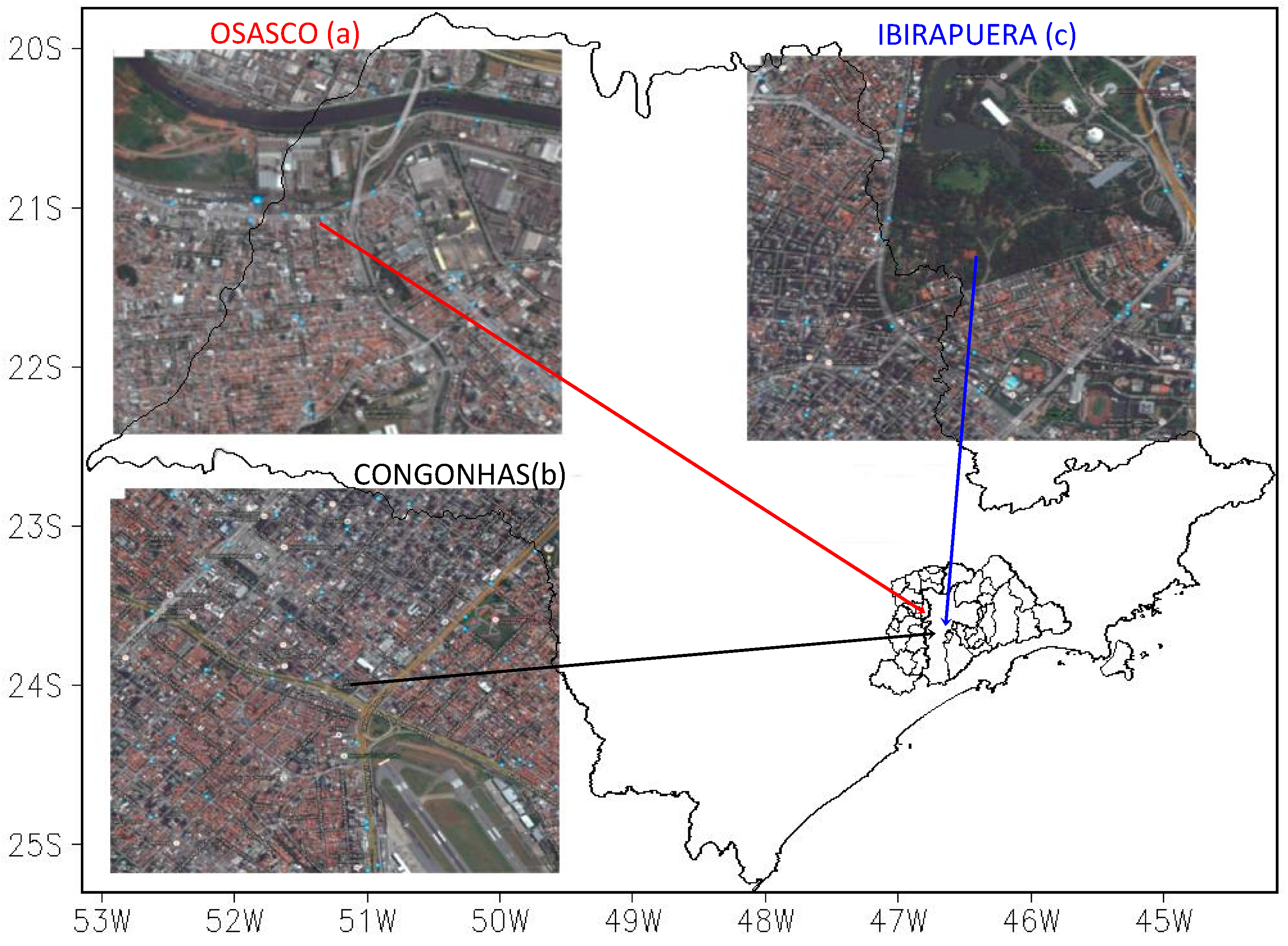
2.1. Characterization of Monitoring Stations

Osasco station (Figure 2a) is in the western portion of the MRSP, in a residential, commercial and industrial area. This station is located approximately 20 m from Autonomistas Avenue, and 45 m from Visconde de Nova Granada Avenue. Both avenues have intense traffic of light and heavy-duty vehicles. So, this station is directly influenced by vehicular emissions.
Congonhas station is located in the south of MRSP, in a commercial and residential area (Figure 2b). This station is approximately 6 m from Avenida dos Bandeirantes and 400 m from Congonhas National Airport. It is also strongly affected by heavy-duty vehicle traffic.
Also located in the south of the MRSP, and approximately 3000 m from the Congonhas station, Ibirapuera station is located (Figure 2c) in a city park surrounded by urbanized areas where the predominant characteristics are residential. This station is approximately 500 m from the Republica do Líbano Avenue and 750 m from Ibirapuera Avenue, so it is not directly influenced by these sources. More information can be found in Table 2.
Clearly, these three stations do not represent the whole intra-urban variability of CO emissions, concentrations and urban conditions in the MRSP area. However, this can be an extremely difficult task and is outside the scope of this study. Despite this fact, the three chosen monitoring stations represent typical conditions of regions directly impacted by (Congonhas, Osasco) or removed from (Ibirapuera) CO emissions throughout the city. So, instead of analyzing too many stations in a shorter time period, we decided to focus on a few long-term monitoring stations in order to capture, more significantly, its temporal evolution and variations in different time scales. This would allow for identifying more clearly the different patterns and cycles of relevance for CO concentration in a variety of time scales and and their association to different factors such as atmospheric conditions and traffic circulation.

2.2. Data

In this study, 16 years of air quality data were used, from January 2000 to December 2015. The samples were averages of hourly frequency. Information on CO concentrations, in part per million (ppm), was obtained from the database of the São Paulo State Environmental Protection Agency (CETESB), in the Air Quality Monitoring department (ar.cetesb.sp.gov.br/qualar/). CETESB obtains the concentrations of this pollutant using an automatic monitoring network connected to a central computer through the telemetry system. Information, recorded on an uninterrupted basis, is processed based on the average established by legal standards and are made available every hour. At 5 o’clock in the morning (local time) there is an automatic calibration of the equipment, so there are no measurements for CO at this hour.
The method used to measure CO concentration is the non-dispersive infrared. It consists of the absorption of radiation by CO. The interaction of this gas with the incident radiation emits energy in the infrared region, so these interactions are detected electronically, amplified and, consequently, quantified. The results are in simple average terms. The analysis of the collected data was performed in terms of annual, monthly, weekly and diurnal cycles.

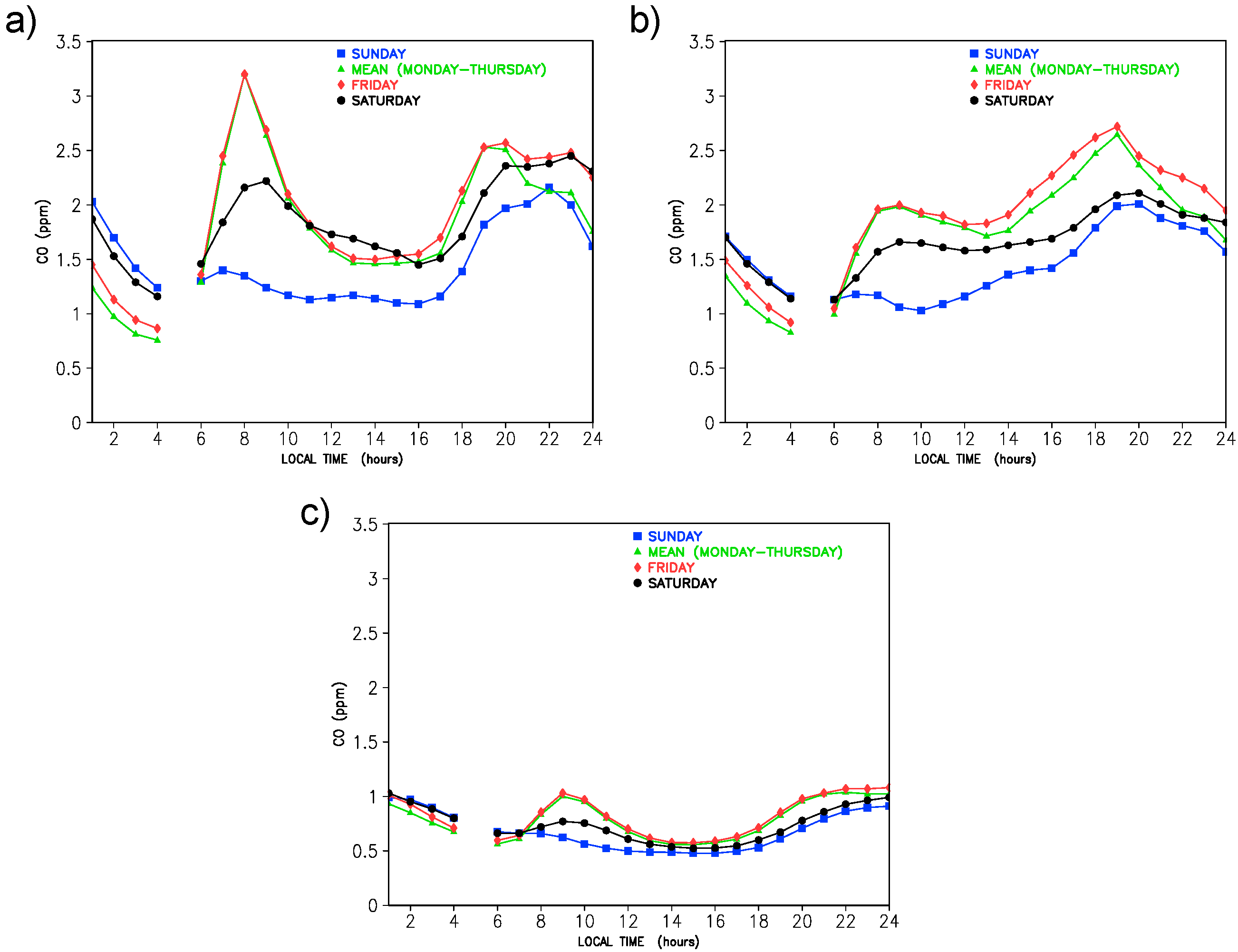
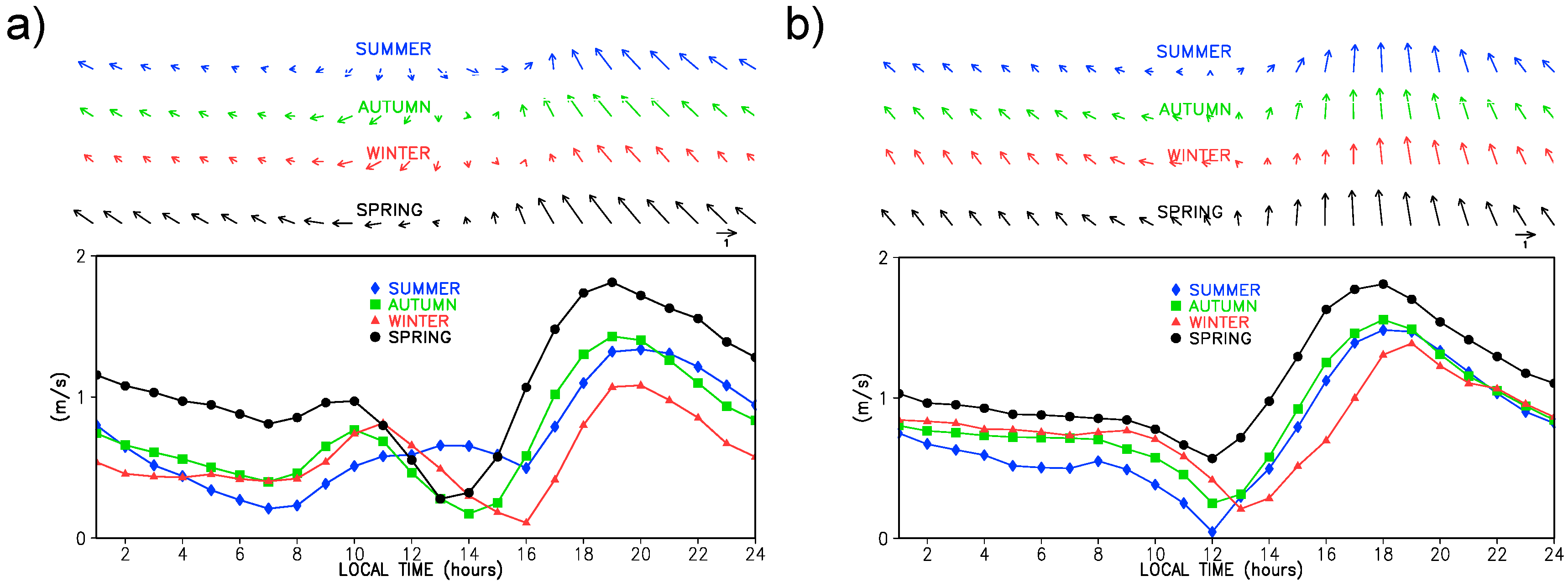
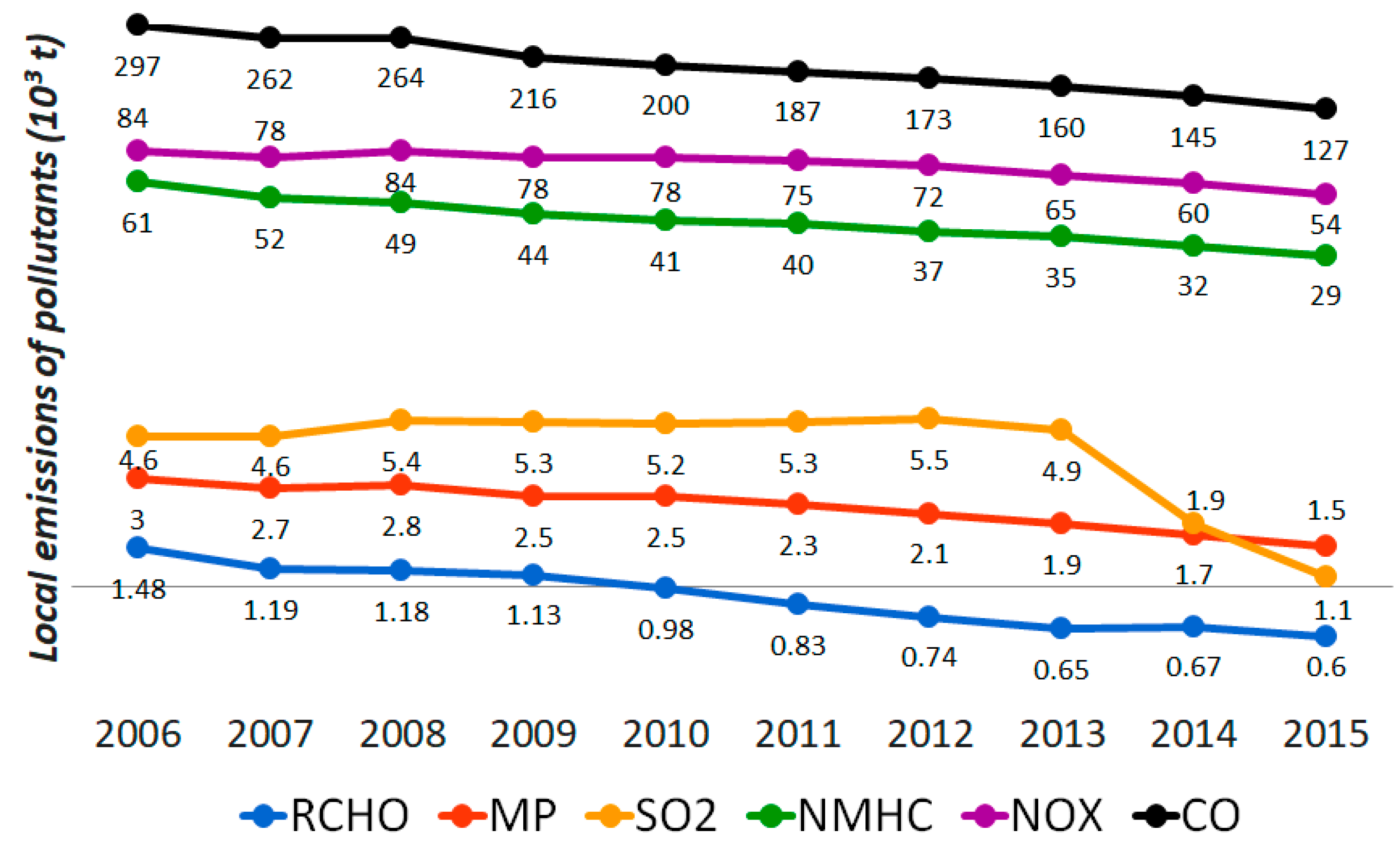
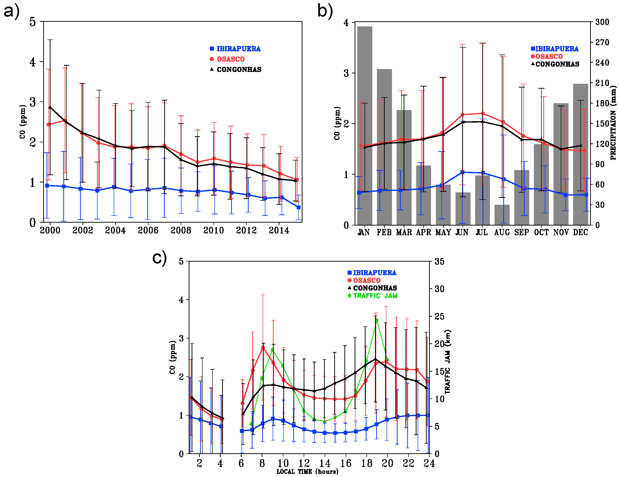
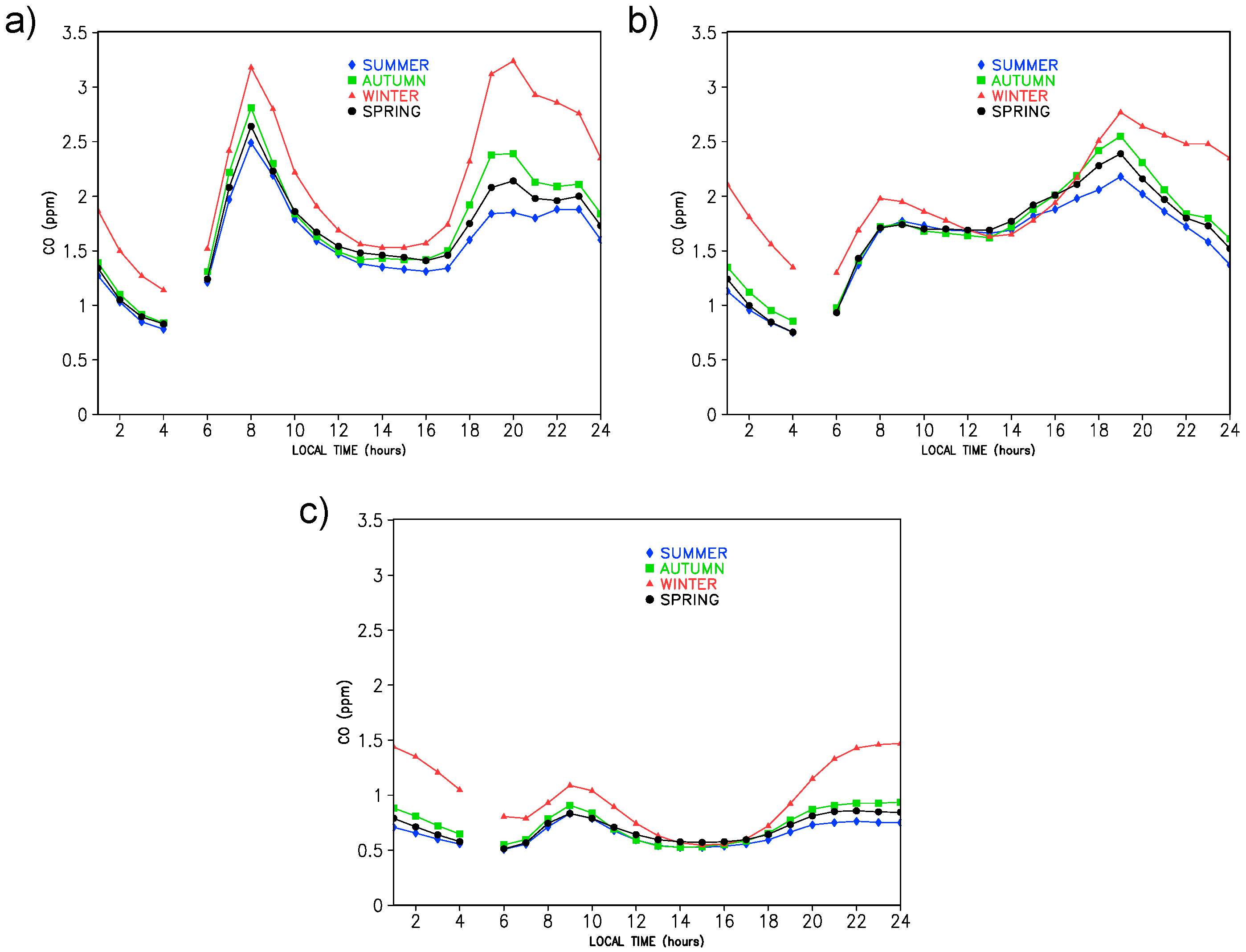
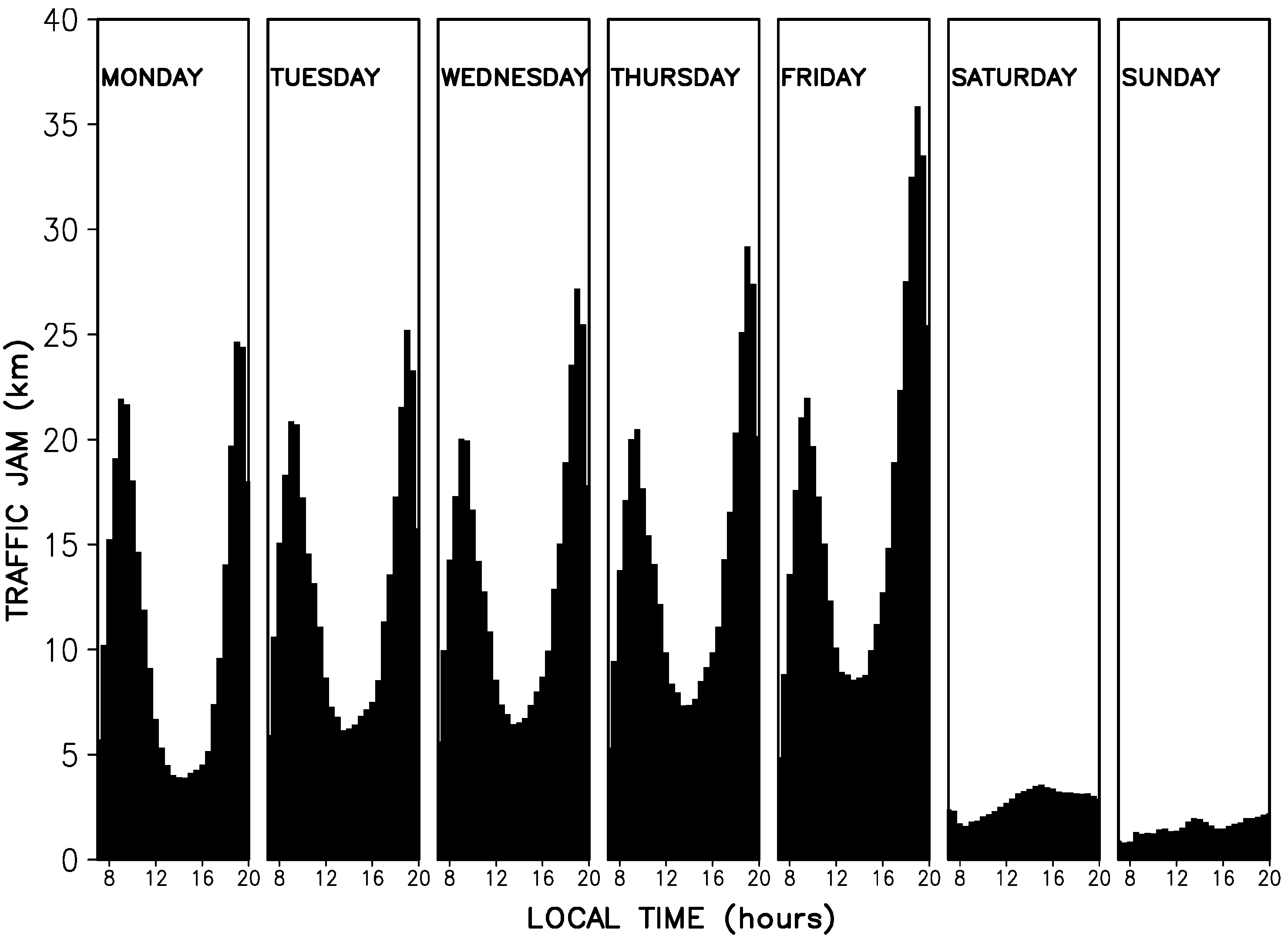
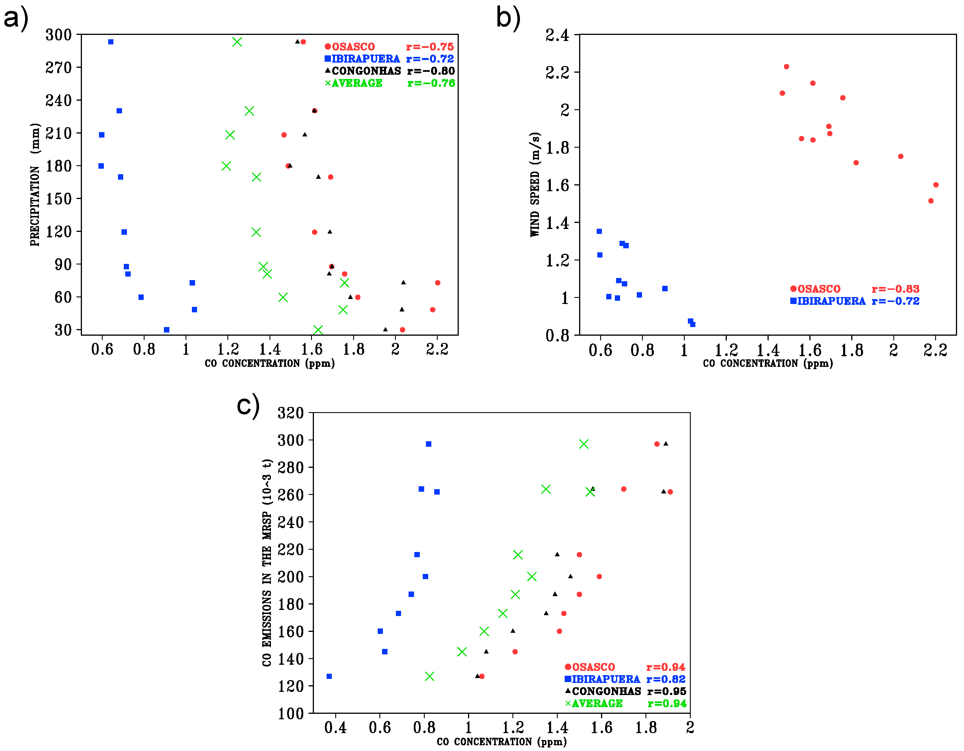
3. Results and Discussion

Figure 3a shows the CO concentration time series for annual means (ppm); (b) monthly CO and cumulative precipitation average and (c) hourly CO averages for monitoring stations Osasco, Congonhas and Ibirapuera Park, and traffic length (km) in São Paulo city measured by the local Traffic Engineering Company (CET), for the same period of the CO measurements (2000 to 2015).
Figure 4 shows average diurnal cycle for Osasco (a), Congonhas (b) and Ibirapuera Park (c), separated by seasons (summer, autumn, winter and spring).
The average diurnal cycle of CO for Osasco (a), Congonhas (b) and Ibirapuera Park (c), separated by day of the week, is shown in Figure 5.
In Figure 6, the average hourly traffic jam distribution (km) in São Paulo city measured by the Traffic Engineering company (CET) during weekdays and weekends for the CO sampled regions is shown.
Figure 7 shows wind speed (m s−1) at CETESB stations (a) Osasco and (b) Ibirapuera, from 2000 to 2015 (where the monitoring sites of CO are located).
In Figure 8, correlation coefficient (𝑟) between monthly averages of precipitation, wind speed and CO emission with CO concentration are presented.

Annual Evolution and Seasonal, Diurnal Cycle

The annual time series for Osasco, Congonhas and Ibirapuera Park stations, Figure 3a, were obtained by averaging all CO concentrations for each year. In general, a decrease in CO concentrations is perceived for the three studied localities. Osasco and Congonhas presented marked decreases, mainly in the first five years. For Ibirapuera, the decrease is smoother. Reductions in CO concentration over the years were also observed in other locations such as in Pt Barrow, Alaska; Cape Meares, Oregon; Cape Kumukahi and Mauna Loa Observatory, Hawaii; Cape Matatula, Samoa; Cape Grim, Tasmania; Palmer Station and South Pole, Antarctica. This decrease is now found largely confined to the Northern Hemisphere, where dramatic reductions in fossil fuel emissions have reportedly occurred. In contrast, no significant trend is determined in the Southern Hemisphere between 1991 and 2001. Globally averaged CO exhibits large interannual variability, primarily reflecting year to year changes in emissions from biomass burning. This behavior may be explained by the reduction of emissions from cars (and industrial sources) due to technological upgrades of vehicle emissions, since the number of vehicles in this region has grown considerably during these years (exemplified in Figure S1). The rate of decrease in CO concentration from 2000 to 2015 was about 63.7% for Congonhas; 56.5% Osasco; and 59.5% for Ibirapuera. Osasco and Congonhas stations had higher CO concentration because they are located close to very busy avenues, under daily direct influence of emissions from thousands of vehicles. Ibirapuera station had the lowest values in concentration over the years and also showed the lowest variation (except for the last year) because it is located in the middle of a park, and the majority of the concentrations measured are probably associated to advective processes which transport CO from adjacent neighborhoods. In the average for all 16 years, in percentage terms, Osasco presented the highest CO concentration: 56% higher than Ibirapuera and 3% higher than of Congonhas. The data shows a decreasing annual trend for CO. They can mostly be related to the Brazilian Vehicular Emission Control Program, which responded for a decrease of 90% and 80% in emissions by light and heavy-duty vehicles, respectively (Figure 1, Figure 3a and Figure 8c).
Figure 3b shows the monthly average of CO concentrations for the three localities studied and the monthly cumulative precipitation. A well-defined seasonal cycle of CO concentration, also verified in many other studies, is clearly observed [42,43]. This cycle presents maximum CO concentrations during June, July and August (JJA), associated with the lowest precipitation ratios during the year. November, December, January and February (NDJF) present the lowest CO concentrations. During these months, high precipitation rates contribute to remove CO from the atmosphere through wet scavenging and convective processes. In the NDJF period, temperatures are higher due to the greater incidence of solar radiation in the ausral summer. This leads to higher rainfall rates by increasing the intensity of the surface-atmosphere flows and strengthening convection; also, moisture content in the air increases due to the prevailing northwest wind directions that also transport humidity from the Amazon Basin region to São Paulo in this period. This brings about the formation of more pronounced upward vertical movements, generating more convection and an efficient advection of pollutants from lower to higher atmospheric levels. On the other hand, during JJA, lower temperatures do not favor thermally induced vertical movements, keeping atmospheric pollutants at lower levels.
Moreover, other atmospheric conditions such as precipitation, wind speed, temperature, relative humidity all contribute to the modulation of the CO seasonal cycle. As seen in the Figure 8a,b precipitation and wind speed have strong inverse correlation with CO. In the Osasco station the correlation of wind speed and CO is higher than in the Ibirapuera station, indicating that the wind is more correlated with CO when its velocity is higher. The wind speed at the Osasco station is on average 40% higher than at Ibirapuera for all months of the analyzed period. In both stations the wind speed is lower during the months of May, June and July and higher during the months of September, October, November and December (Figure 7 and Tables S2 and S3). The lowest values of precipitation for the analyzed period occur in the months of May, June and August and the highest concentrations of CO occur in the months of June, July, August (Figure 3b and Table S1). Wind speed varies little during the year with an average of (1.08 ± 0.16 m s−1) for Ibirapuera and (1.87 ± 0.22 m s−1) Osasco station, while precipitation has a high variation throughout the year (132 ± 83 mm) and the monthly average of CO concentration for the three stations was (1.42 ± 0.20 ppm). High wind speeds enhance the turbulence and increase the dispersion and transport of CO, decreasing its concentration. When the wind speed is low, the CO emitted tends to concentrate near its sources.
Concerning the temperature, the months of June/July in the Megacity of São Paulo present generally lower values, when the concentrations of pollutants are higher (except for ozone). In this situation, conditions of atmospheric stability are more likely to take place. Critical episodes of air pollution occur during the dry period (except for ozone), under the influence of the subtropical atlantic anticyclone (a high-pressure system) which prevents the cold fronts from reaching the MRSP, limiting their influence to south of the state of Sao Paulo. These synoptic circumstances influence the meteorological conditions in this region, causing a decrease in wind speed (which are usually less than 1.5 m s−1) and many hours of calm winds (wind speed on surface less than 0.5 m s−1), as seen in Figure 7. Clear sky conditions prevail, together with great atmospheric stability and the formation of thermal inversion layers very close to the surface (below 200 m). These conditions are unfavorable for the dispersion of the pollutants emitted in the Megacity of São Paulo. Normally, this situation of atmospheric stagnation is disturbed by the onset of a new air mass in the region associated with a frontal system, increasing ventilation, instability and, in many cases, causing precipitation. Another peculiarity is that the relative humidity in the dry period reaches values of 15%. During the studied period, June, July and August presented days of low relative humidity, below 30%, which also presented calm, weak winds and thermal inversion layers at low levels. This atmospheric stability causes great respiratory discomfort to the population [2] and also inhibits the dispersion of CO, consequently, increasing its concentration, which might lead to higher respiratory discomfort for the population.
The seasonal pattern of CO is also associated with chemical reactions occurring in the troposphere. In this context, the seasonal CO cycle is also modulated by the seasonal cycle of the hydroxyl (OH) radical present in the troposphere. According to [44], hydroxyl concentration maximums were observed in the austral summer, which correspond to minimum CO concentration. Background OH is high in summer and low in winter, as a consequence of the solar radiation variation. Concentrations of OH are highest in the tropics where water vapor and UV radiation are high because of opposite vertical trends of water vapor (decreasing with altitude) and UV radiation (increasing with altitude). Concentrations of OH tend to be higher in urban area than because of higher O3 and NOx, stimulating OH production; this effect compensates for the faster loss of OH due to elevated CO. The diurnal variations of OH and HO2 were measured in the comparison of four field studies: TEXAQS2000 (Houston, 2000), NYC2001 (New York City, 2001), MCMA2003 (Mexico City, 2003), and TRAMP2006 (Houston, 2006) showing the expected peak value during midday [45]. The differences in the midday OH abundances are about a factor of 3 for the four studies, which is not surprising considering the differences in photolysis rates and precursor atmospheric constituents. The presence of OH radicals in the troposphere contribute to the removal of CO and other polluting gases. Hydroxil levels are much higher in the boundary layer than in the upper troposphere, and higher in summer than in winter. Thus, these large-scale seasonal changes observed in the chemical composition of the atmosphere, specially through the concentration of OH, might also impact CO lifetime in the boundary layer, making it shorter in summer than in winter, together with the above mentioned active meteorological conditions.
Hydrocarbons emission ratios are higher in summer due to evaporation, and also in winter (together with CO) due to the incomplete burning of fossil fuels and biofuels from vehicle exhaust. Low temperatures also contribute to high CO concentrations. Engines and vehicle emissions-control equipment operate less efficiently when the air is cold: air-to-fuel ratios are lower, combustion is less complete, and catalysts take longer to become fully operational. The result is that products of incomplete combustion, including CO, are formed in higher concentrations. Often, the topography, meteorology, and emissions combine to determine high concentrations of CO in the MRSP. Concerning the emission of thermal NOx, lower ambient temperature also causes it to decrease. All these facts show the influence of meteorological conditions on emissions, and, therefore, the necessity of greater attention from public managers and policymakers to these issues during the winter months.
Figure 3c shows the average diurnal cycle of CO concentration for the three studied sites. The values represent the average for each hour (except at 05 local time) of every day during the studied period. There are two peaks of concentration for Osasco and Congonhas: the first at 8 and 9 h and the second at 19 and 20 h for Osasco (2.76 and 2.36 ppm) and Congonhas (1.79 and 2.46 ppm). It is associated to the rush hour when people commute (see Figure 3c). Other studies, such as [46,47] found these same patterns for the CO daily cycle, as did [48] for downtown Sao Paulo. In Ibirapuera Park station, the peaks occur at 9 and 24 h (0.91 and 1.00 ppm). This station presents the lowest values of concentration and lowest variability. Because the station is inside a park, there is no direct influence from vehicular emission. The CO measured in this station is probably associated to the advection of emission from roads in adjacent regions (see Figure 2).
A Swedish study between 1991 and 2002, in which 2725 nonsmokers aged 18–60 years were evaluated, showed that those who lived in more polluted areas had a greater risk of developing asthma (about 30% for each increase of 1 μg m−3 in PM10 concentration emitted by traffic) [49]. As observed in Figure 2, Ibirapuera station, 500 and 750 m far from the vehicular traffic routes, has average CO concentrations 56% lower than the Osasco stations, approximately 20 and 45 m far from main routes, 53% lower than Congonhas, that is located approximately 6 m from Avenida dos Bandeirantes and 400 m from Congonhas National Airport. Public health laws are designed to protect the most susceptible population groups. The U.S. Environmental Protection Agency (EPA) indicates that attainment of the ambient-CO standards can decrease morbidity and mortality from atherosclerotic heart disease [50]. People with coronary artery disease or other cardiopulmonary diseases, smokers, fetuses, infants, elderly and athletes who exercise heavily in high-CO atmospheres are particularly susceptible to experiencing adverse health effects from CO. Although less conclusive, there is evidence that attainment of the CO standards will also decrease morbidity from pulmonary disease, neurological disease, fetal loss, and childhood developmental abnormalities. These health benefits translate into economic savings associated with avoided health care and avoided work-time losses as well as intangible savings in life quality. This data emphasizes the importance of monitoring air quality in large urban centers as São Paulo, for decision-making in terms of housing construction and exposure profile of the population in their workplaces and regions where they live. Considering the 15 stations that measure CO in the MRSP, Osasco and Congonhas have the fifth and sixth largest CO concentrations, respectively, and the Ibirapuera station, the ninth. It is important to point out that, in the Megacity of São Paulo, stations with higher concentrations of pollutants such as CO, NOx and SO2 (PM2.5/PM10 to a certain extent), ozone concentrations are lower, and the reverse occurs for stations with higher concentrations of O3 [2,39]. Considering all 20 air quality monitoring stations in the MRSP, Ibirapuera station has the second highest ozone concentration. As O3 is a secondary pollutant, the highest ozone concentrations are observed downwind from the emission sources of its precursors (VOCs, CO and NOx), sometimes many miles downwind. The most important ozone precursors source in the MRSP are vehicle emissions [37]. In urban and suburban areas, anthropogenic VOCs emissions prevail and, in conjunction with anthropogenic NOx emissions, lead to peak concentrations of ozone observed in urban areas and regions downwind of major cities [3,5,37].
Figure 4 shows the average diurnal cycle for the three sites separated by season. In Osasco (Figure 4a), the highest concentrations were observed during winter at all hours of the diurnal cycle, and the lowest, in summer. During the night and early morning, the differences between the other seasons were more significant. The peak of CO concentration occurs in the morning (8 h) during autumn, spring and summer, whereas in winter, its magnitude is similar to that of the nocturnal peak (20 h) (both around 3.2 ppm). Congonhas (Figure 4b) shows higher concentrations in winter during almost the whole cycle, except for the hours between 12 and 17 local time. The differences are most significant during the night and early morning hours. It indicates two peak concentrations, the first occurring at 8 h and the second (with higher values) at 19 h. For Ibirapuera (Figure 4c) the concentrations referring to summer and spring present similar patterns, but with small differences in magnitude (about 7% during night/early morning and 4% during the day). The most relevant differences occurred in winter, when the concentration is higher during most hours of the day, except between 13 and 17 h (period in which all seasons have similar values). In general, the highest concentrations occurred during winter, and the lowest in summer, with the most significant differences between the seasons occurring during the night and early morning.
Concerning the weekly cycle, Osasco station (Figure 5a) also presented the highest CO concentrations among the analyzed stations. All stations presented similar CO concentrations for weekdays between 6 and 19 h, except on Friday, due to the greater number of vehicles in the MRSP, which promoted higher concentrations at some hours of the day (see Figure 6). After 20 h, Friday had higher concentrations comparing to the rest of the week (on average, 20% higher compared to other days of the week between 20 and 24 h). On Saturdays, there is a decrease in the morning peak, and a displacement of the maximum nocturnal peak. Moreover, between 12 and 15 h, the concentrations are highest than all other days, associated to an increase in traffic (Figure 6). On Sundays, the highest concentrations occur in the first hours of the day (between 1 and 4 h), when they are higher than on weekdays, but at other times the concentrations are lower.
In Congonhas station (Figure 5b), a similar behavior occurs in the diurnal cycle during weekdays, with the peaks of maximum concentration occurring at 9 and 19 h. Among the weekdays, especially after 12 h, the lowest values of concentration were measured on Mondays, while the highest, on Friday. In the first six hours of the day, there are similar concentrations on Saturday and Sunday, and higher than the rest of the weekdays. After 7 AM, the behavior changes, i.e., CO concentrations are higher for weekdays and lower on weekends, with lower values attributed to Sundays due to the lesser number of vehicles circulating in the city.
For Ibirapuera Park (Figure 5c), the weekdays presented similar magnitude and behavior in the diurnal cycle. On weekends, there is a slight decrease in CO concentration, especially during rush hours (7 to 9 AM and 18 to 20 h at night), with the lowest concentrations on Sunday. In general, weekends present higher values of CO concentrations in the first four hours of the day (results similar to those of [30]). This fact is due to the high emissions at the end of the night of the previous days (Friday and Saturday). In the other hours of the cycle, the lowest concentrations are on Sundays, and the highest on Friday due to higher vehicular emission. On Saturdays, except for Ibirapuera Park, there was a distinctive behavior between the hours of 12 and 14 h. During these hours, there is usually a sharp decrease in concentrations (due to increased turbulence in the boundary layer during the afternoon); however, this decrease is not observed in Congonhas station, and in Osasco station, the decrease is less pronounced compared to weekdays. This is due to an increase in the vehicles traveling which is shown in Figure 6. In Congonhas station, this might be related to the busy airport located nearby this monitoring point, which increases local traffic due to the relatively constant flow of passengers over time.

4. Conclusions

The behavior of the annual, seasonal, weekly and daily variations of CO concentration in the Megacity of São Paulo were prospectively studied. Based on the results, we concluded that in terms of annual variations, CO concentrations decreased in all studied sites, in 0.114, 0.086 and 0.034 ppm per year−1 for Congonhas, Osasco and Ibirapuera, respectively. This trend in the reduction of CO over the years is attributed mainly to the decrease in vehicle emissions due to new technologies and the implementation of environmental laws which demand that the car manufacturers comply with the standards of emission enforced by public agencies, since the vehicle fleet has increased every year. Similar results were also observed in other studies for other locations [15,51]. Among the localities analyzed in this study, Osasco and Congonhas presented the highest levels of CO concentration, however, also indicated the greatest decreases. The high concentration of this pollutant for these two stations is due their location, close to avenues with intense vehicular traffic. Ibirapuera station, because it is located inside a park and more distant from the roads, presented the lowest values of concentrations when compared to the other stations (around 55% considering the average among 16 years).
In terms of seasonal variations, the maximum values of CO concentrations occurred in June and July (winter), while the lowest, in December, January and February (summer). This behavior is mainly due to meteorological and chemical factors. In terms of weather, the months of December and January (summer) are characterized by high temperature and precipitation ratios that provide unstable atmospheric conditions, promoting the dispersion or removal of CO. In this case, the dispersion is mainly due to the convective and turbulent processes in the boundary layer, while the removal, to the high rainfall ratio. In June, July and August (winter), higher atmospheric pressure and lower temperatures are associated to more stable atmospheric conditions and less rainfall. A lower planetary boundary layer reduces the convective and turbulent processes, and together with low rainfall rates, hinders CO dispersion. The daily CO concentration evolution in urban regions is directly related to the temporal evolution of vehicular traffic and the local meteorological conditions such as the height of the thermal inversion and the intensity of the atmospheric turbulence [27,28].
In general, the diurnal cycle of CO concentration presents two peaks, in the morning (between 8 and 9 h) and in the early evening (between 19 and 20 h). These maximum concentration values occur due to the heavy traffic of motor vehicles at these hours. Another important factor is the low efficiency (low turbulence) of the planetary boundary layer in dispersing the CO in these two periods of the day. In the early hours of the morning, motor vehicle traffic is intense and surface heating by solar radiation is still not enough to break the previous night’s thermal inversion layer, causing the pollutants to remain concentrated in regions close to the surface. After 10 a.m., the intensity of the traffic decreases and the growth of the PBL increases allowing the transport of the to the upper layers due to the strong convective activity, which favors the dispersion throughout the layer. As a result, the concentration levels on the surface decrease and rise again by the end of the afternoon, when convective activity decreases and motor vehicle traffic intensifies.
The diurnal cycle analysis of each day of the week clearly shows the impact of the vehicular traffic on the diurnal variation of CO concentration levels. On weekdays, a similar behavior is observed, except after 20 h. For these times, in most locations, Friday presents the highest CO concentrations. This feature is directly associated with highest traffic congestion according to the traffic engineering company. On Sundays, peaks occurred at night because of the return of vehicular traffic at the end of the weekend. For the first hours of the day (between 1 and 4 h), weekends present higher values of CO concentration due to the contribution of the previous day’s emissions and greater atmospheric stability during the nighttime. The diurnal cycle of CO concentration, analyzed for each season of the year, shows that the amount of CO in the atmosphere is higher during the winter months, followed by autumn and spring, with the lowest concentration observed during summer months.

Supplementary Materials

The following are available online at www.mdpi.com/2073-4433/8/5/81/s1, Table S1: Monthly cumulative precipitation at IAG/USP station, Table S2: Monthly average wind speed at Osasco station, Table S3: Monthly average wind speed at Ibirapuera station, Figure S1: Evolution of vehicle fleet in São Paulo city. Source: São Paulo State Traffic Department (Detran-SP).

Acknowledgments

The authors express their gratitude for Conselho Nacional de Desenvolvimento Científico e Tecnológico—CNPQ (National Counsel of Technological and Scientific Development) (No. 800012/2016-0) for providing the fellowship for Vinicius Rozante and Coordenação de Aperfeiçoamento de Pessoal no Nível Superior—CAPES (Coordination for the Improvement of Higher Level Personnel) (No. 88887.115872/2015-01) for providing the postdoc fellowship for Débora Souza Alvim. We are grateful for CETESB for providing us with the monoxide carbon data and the Companhia de Engenharia de Tráfego—CET (Traffic Engineering Company) for providing us with the traffic data.

Author Contributions

José Roberto Rozante, Vinícius Rozante, Débora Souza Alvim defined the location of the data sites and downloaded the data; José Roberto Rozante, Vinícius Rozante, Débora Souza Alvim, Júlio Barboza Chiquetto, Antônio Manzi, Monica Siqueira D’Amelio and Demerval Soares Moreira contributed to the interpretation of the data analysis. José Roberto Rozante, Vinícius Rozante, Débora Souza Alvim, Júlio Barboza Chiquetto, Antônio Manzi, Monica Siqueira D’Amelio wrote the paper; Vinícius Rozante, Júlio Barboza Chiquetto, Antônio Manzi, Monica Siqueira D’Amelio contributed to the design of the study and revised the paper.

Conflicts of Interest

The authors declare no conflict of interest.

References

  1. Brazilian Institute of Geography and Statistics. IBGE 2014: Brazilian Census; Brazilian Institute of Geography and Statistics: Paulo Rabello de Castro, Brazil, 2015.
  2. Environmental Agency of the State of São Paulo. CETESB: Air Quality Report in São Paulo—2015; Environmental Agency of the State of São Paulo: São Paulo, Brazil, 2016.
  3. Finlayson-Pitts, B.J.; Pitts, J.N. Chemistry of the Upper and Lower Atmosphere—Theory, Experiments, and Applications, 1st ed.; Academic Press: San Diego, CA, USA, 2000. [Google Scholar]
  4. Wofsy, S.C.; McConnell, J.C.; McElroy, M.B. Atmospheric CH4, CO, and CO2. J. Geophys. Res. 1972, 77, 4477–4493. [Google Scholar] [CrossRef]
  5. Seinfeld, J.H.; Pandis, S.N. Atmospheric Chemistry and Physics: From Air Pollution to Climate Change, 3rd ed.; Wiley: Hoboken, NJ, USA, 2016. [Google Scholar]
  6. Horowitz, L.W.; Walters, S.; Mauzerall, D.L.; Emmons, L.K.; Rasch, P.J.; Granier, C.; Tie, X.; Lamarque, J.F.; Schultz, M.G.; Tyndall, G.S.; et al. A global simulation of tropospheric ozone and related tracers: description and evaluation of mozart, version 2: Mozart-2 description and evaluation. J. Geophys. Res. Atmos. 2003, 108. [Google Scholar] [CrossRef]
  7. Bakwin, P.S.; Tans, P.P.; Novelli, P.C. Carbon monoxide budget in the northern hemisphere. Geophys. Res. Lett. 1994, 21, 433–436. [Google Scholar] [CrossRef]
  8. Levy, H. Normal Atmosphere: Large Radical and Formaldehyde Concentrations Predicted. Science 1971, 173, 141–143. [Google Scholar] [CrossRef] [PubMed]
  9. Crutzen, P.J.; Zimmermann, P.H. The changing photochemistry of the troposphere. Tellus A 1991, 43, 136–151. [Google Scholar] [CrossRef]
  10. DeMore, W.B.; Sander, S.P.; Golden, D.M.; Hampson, R.F.; Kurylo, M.J.; Howard, C.J.; Ravishankara, A.R.; Kolb, C.E.; Molina, M.J. Chemical Kinetics and Photochemical Data for Use in Stratospheric Modeling. Evaluation No. 12. Available online: https://ntrs.nasa.gov/archive/nasa/casi.ntrs.nasa.gov/19970037557.pdf (accessed on 20 April 2017).
  11. Sze, N.D. Anthropogenic CO Emissions: Implications for the Atmospheric CO-OH-CH4 Cycle. Science 1977, 195, 673–675. [Google Scholar] [CrossRef] [PubMed]
  12. Jacobson, M.Z. Atmospheric Pollution: History, Science, and Regulation, 1st ed.; Cambridge University Press: Cambridge, UK, 2002. [Google Scholar]
  13. Isaksen, I.S.A.; Hov, Ø. Calculation of trends in the tropospheric concentration of O3, OH, CO, CH4 and NOx. Tellus Ser. B 1987, 39, 271–285. [Google Scholar] [CrossRef]
  14. Zander, R.; Demoulin, P.; Ehhalt, D.H.; Schmidt, U.; Rinsland, C.P. Secular increase of the total vertical column abundance of carbon monoxide above central Europe since 1950. J. Geophys. Res. 1989, 94, 11021. [Google Scholar] [CrossRef]
  15. Khalil, M.A.K.; Rasmussen, R.A. Global decrease in atmospheric carbon monoxide concentration. Nature 1994, 370, 639–641. [Google Scholar] [CrossRef]
  16. Thompson, A.M.; Cicerone, R.J. Atmospheric CH4, CO and OH from 1860 to 1985. Nature 1986, 321, 148–150. [Google Scholar] [CrossRef]
  17. Wang, C.; Prinn, R.G.; Sokolov, A. A global interactive chemistry and climate model: Formulation and testing. J. Geophys. Res. Atmos. 1998, 103, 3399–3417. [Google Scholar] [CrossRef]
  18. Kanakidou, M.; Crutzen, P.J. The photochemical source of carbon monoxide: Importance, uncertainties and feedbacks. Chemosphere Glob. Chang. Sci. 1999, 1, 91–109. [Google Scholar] [CrossRef]
  19. Jaffe, L.S. Ambient carbon monoxide and its fate in the atmosphere. J. Air Pollut. Control Assoc. 1968, 18, 534–540. [Google Scholar] [CrossRef] [PubMed]
  20. Cançado, J.E.D.; Braga, A.; Pereira, L.A.A.; Arbex, M.A.; Saldiva, P.H.N.; Santos, U.P. Clinical repercussions of exposure to atmospheric pollution. J. Bras. Pneumol. 2006, 32, S5–S11. [Google Scholar] [CrossRef] [PubMed]
  21. Raub, J.A.; Mathieu-Nolf, M.; Hampson, N.B.; Thom, S.R. Carbon monoxide poisoning—A public health perspective. Toxicology 2000, 145, 1–14. [Google Scholar] [CrossRef]
  22. Coburn, R.F. The carbon monoxide body stores. Ann. N. Y. Acad. Sci. 1970, 174, 11–22. [Google Scholar] [CrossRef] [PubMed]
  23. Medeiros, A.; Gouveia, N. Relationship between low birthweight and air pollution in the city of Sao Paulo, Brazil. Rev. Saúde Pública 2005, 39, 965–972. [Google Scholar] [CrossRef] [PubMed]
  24. Friedman, M.S. Impact of changes in transportation and commuting behaviors during the 1996 summer olympic games in atlanta on air quality and childhood asthma. JAMA 2001, 285, 897. [Google Scholar] [CrossRef] [PubMed]
  25. Li, Y.; Wang, W.; Kan, H.; Xu, X.; Chen, B. Air quality and outpatient visits for asthma in adults during the 2008 Summer Olympic Games in Beijing. Sci. Total Environ. 2010, 408, 1226–1227. [Google Scholar] [CrossRef] [PubMed]
  26. Morgenstern, V.; Zutavern, A.; Cyrys, J.; Brockow, I.; Koletzko, S.; Krämer, U.; Behrendt, H.; Herbarth, O.; von Berg, A.; Bauer, C.P.; et al. Atopic diseases, allergic sensitization, and exposure to traffic-related air pollution in children. Am. J. Respir. Crit. Care Med. 2008, 177, 1331–1337. [Google Scholar] [CrossRef] [PubMed]
  27. Oliveira, A.P.; Bornstein, R.D.; Soares, J. Annual and diurnal wind patterns in the city of são paulo. Water Air Soil Pollut. Focus 2003, 3, 3–15. [Google Scholar] [CrossRef]
  28. Bogo, H.; Gómez, D.R.; Reich, S.L.; Negri, R.M.; Román, E.S. Traffic pollution in a downtown site of Buenos Aires City. Atmos. Environ. 2001, 35, 1717–1727. [Google Scholar] [CrossRef]
  29. De Oliveira, A.P.; Machado, A.J.; Escobedo, J.F.; Soares, J. Diurnal evolution of solar radiation at the surface in the city of São Paulo: Seasonal variation and modeling. Theor. Appl. Climatol. 2002, 71, 231–249. [Google Scholar] [CrossRef]
  30. Sailor, D.J.; Fan, H. Modeling the diurnal variability of effective albedo for cities. Atmos. Environ. 2002, 36, 713–725. [Google Scholar] [CrossRef]
  31. Oke, T.R. Boundary Layer Climates, 2rd ed.; Routledge: New York, NY, USA, 1988. [Google Scholar]
  32. Cai, X.M. Large-eddy simulation of the convective boundary layer over an idealized patchy urban surface. Q. J. R. Meteorol. Soc. 1999, 125, 1427–1444. [Google Scholar] [CrossRef]
  33. Martins, M.H.R.B.; Anazia, R.; Guardani, M.L.G.; Lacava, C.I.V.; Romano, J.; Silva, S.R. Evolution of air quality in the Sao Paulo metropolitan area and its relation with public policies. Int. J. Environ. Pollut. 2004, 22, 430. [Google Scholar] [CrossRef]
  34. Carvalho, V.S.B.; Freitas, E.D.; Martins, L.D.; Martins, J.A.; Mazzoli, C.R.; Andrade, M.F. Air quality status and trends over the Metropolitan Area of São Paulo, Brazil as a result of emission control policies. Environ. Sci. Policy 2015, 47, 68–79. [Google Scholar] [CrossRef]
  35. Martins, L.D.; Martins, J.A.; Freitas, E.D.; Mazzoli, C.R.; Gonçalves, F.L.T.; Ynoue, R.Y.; Hallak, R.; Albuquerque, T.T.A.; Andrade, M.F. Potential health impact of ultrafine particles under clean and polluted urban atmospheric conditions: A model-based study. Air Qual. Atmos. Health 2010, 3, 29–39. [Google Scholar] [CrossRef] [PubMed]
  36. Orlando, J.P.; Alvim, D.S.; Yamazaki, A.; Corrêa, S.M.; Gatti, L.V. Ozone precursors for the São Paulo Metropolitan Area. Sci. Total Environ. 2010, 408, 1612–1620. [Google Scholar] [CrossRef] [PubMed]
  37. Alvim, D.S.; Gatti, L.V.; Corrêa, S.M.; Chiquetto, J.B.; Rossatti, C.S.; Pretto, A.; Santos, M.H.; Yamazaki, A.; Orlando, J.P.; Santos, G.M. Main ozone-forming VOCs in the city of Sao Paulo: Observations, modelling and impacts. Air Qual. Atmos. Health 2016. [Google Scholar] [CrossRef]
  38. Massambani, O.; Andrade, F. Seasonal behavior of tropospheric ozone in the Sao Paulo (Brazil) Metropolitan Area. Atmos. Environ. 1994, 28, 3165–3169. [Google Scholar] [CrossRef]
  39. Chiquetto, J.B.; Silva, M.E.S. Sao Paulo’s “Surface Ozone Layer” and the Atmosphere, 1st ed.; VDM Verlag Dr Müller: Saarbrücken, Germany, 2010; Volume 1. [Google Scholar]
  40. Gallardo, L.; Escribano, J.; Dawidowski, L.; Rojas, N.; Andrade, M.F.; Osses, M. Evaluation of vehicle emission inventories for carbon monoxide and nitrogen oxides for Bogotá, Buenos Aires, Santiago, and São Paulo. Atmos. Environ. 2012, 47, 12–19. [Google Scholar] [CrossRef]
  41. Vivanco, M.G.; Andrade, M.F. Validation of the emission inventory in the Sao Paulo Metropolitan Area of Brazil, based on ambient concentrations ratios of CO, NMOG and NOx and on a photochemical model. Atmos. Environ. 2006, 40, 1189–1198. [Google Scholar] [CrossRef]
  42. Seiler, W.; Giehl, H.; Brunke, E.-G.; Halliday, E. The seasonality of CO abundance in the Southern Hemisphere. Tellus B 1984, 36B, 219–231. [Google Scholar] [CrossRef]
  43. Badr, O.; Probert, S.D. Sources of atmospheric carbon monoxide. Appl. Energy 1994, 49, 145–195. [Google Scholar] [CrossRef]
  44. Logan, J.A.; Prather, M.J.; Wofsy, S.C.; McElroy, M.B. Tropospheric chemistry: A global perspective. J. Geophys. Res. 1981, 86, 7210. [Google Scholar] [CrossRef]
  45. Mao, J.; Ren, X.; Chen, S.; Brune, W.H.; Chen, Z.; Martinez, M.; Harder, H.; Lefer, B.; Rappenglück, B.; Flynn, J.; Leuchner, M. Atmospheric oxidation capacity in the summer of Houston 2006: Comparison with summer measurements in other metropolitan studies. Atmos. Environ. 2010, 44, 4107–4115. [Google Scholar] [CrossRef]
  46. McCormick, R.A.; Xintaras, C. Variation of carbon monoxide concentrations as related to sampling interval, traffic and meteorological factors. J. Appl. Meteorol. 1962, 1, 237–243. [Google Scholar] [CrossRef]
  47. Comrie, A.C.; Diem, J.E. Climatology and forecast modeling of ambient carbon monoxide in Phoenix, Arizona. Atmos. Environ. 1999, 33, 5023–5036. [Google Scholar] [CrossRef]
  48. Chiquetto, J.B.; Ynoue, R.Y.; Cabral-Miranda, W.; Silva, M.E.S. Changes in air pollution due to the implementation of urban parks in megacities: Observations and modelling. BPG 2016, 95, 1–24. [Google Scholar]
  49. Kunzli, N.; Bridevaux, P.O.; Liu, L.J.S.; Garcia-Esteban, R.; Schindler, C.; Gerbase, M.W.; Sunyer, J.; Keidel, D.; Rochat, T. Traffic-related air pollution correlates with adult-onset asthma among never-smokers. Thorax 2009, 64, 664–670. [Google Scholar] [CrossRef] [PubMed]
  50. U.S. Environmental Protection Agency. Final Assessment: Integrated Science Assessment for Carbon Monoxide; U.S. Environmental Protection Agency: Washington, DC, USA, 2010.
  51. Novelli, P.C. Reanalysis of tropospheric CO trends: Effects of the 1997–1998 wildfires. J. Geophys. Res. 2003, 108. [Google Scholar] [CrossRef]
Figure 1. Evolution of pollutants emissions in the MRSP.
Atmosphere 08 00081 g001
Figure 2. Location of the three automatic air quality monitoring stations of this study, Osasco (a), Congonhas (b) and Ibirapuera Park (c).
Atmosphere 08 00081 g002
Figure 3. (a) CO concentration time series for annual means (ppm), (b) monthly CO and cumulative precipitation average and (c) hourly CO averages for monitoring stations Osasco, Congonhas and Ibirapuera Park, and traffic length (km) in São Paulo city measured by the local Traffic Engineering Company (CET), for the same period of the CO measurements (2000 to 2015).
Atmosphere 08 00081 g003
Figure 4. Average diurnal cycle for Osasco (a), Congonhas (b) and Ibirapuera Park (c), separated by seasons (summer, autumn, winter and spring).
Atmosphere 08 00081 g004
Figure 5. Average diurnal cycle of CO for Osasco (a), Congonhas (b) and Ibirapuera Park (c), separated by day of the week.
Atmosphere 08 00081 g005
Figure 6. Average hourly traffic jam distribution (km) in São Paulo city measured by the Traffic Engineering company (CET) during weekdays and weekends for the CO sampled regions.
Atmosphere 08 00081 g006
Figure 7. Wind speed (m s−1) at Environmental Agency of the State of São Paulo (CETESB) stations (a) Osasco and (b) Ibirapuera, from 2000 to 2015 (where the monitoring sites of CO are located).
Atmosphere 08 00081 g007
Figure 8. Correlation coefficient (𝑟) between monthly averages of precipitation (a), wind speed (b) and CO emission with CO concentration (c).
Atmosphere 08 00081 g008
Table 1. Emission estimation of air pollution sources in the Metropolitan Region of São Paulo (MRSP) in 2015.
CategoryFuelEmission (1000 t/Year)
Automobiles COHCNOxPMSOx
Gasoline C69.1614.218.790.040.19
Hydrated Ethanol 14.012.621.13nana
Flex-gasoline C9.593.931.040.020.11
Hydrated flex-ethanol11.093.540.95nana
Light commercial vehiclesGasoline C13.192.361.300.0070.04
Hydrated Ethanol0.890.170.08nana
Flex-gasoline C1.380.700.170.0030.02
Hydrated flex-ethanol1.980.570.21nana
Diesel1.050.274.350.180.32
Semi-Light 0.230.071.250.060.03
TrucksLightDiesel1.010.315.730.240.18
Medium
Semi-Heavy
Heavy
0.66
0.81
0.22
0.19
3.84
4.64
0.19
0.14
0.10
0.17
0.740.204.600.140.18
BusesUrban
Mini-bus
Diesel2.44
0.17
0.55
0.04
12.72
0.92
0.37
0.02
0.01
0.001
Intercity 0.230.071.480.020.06
MotorcyclesGasoline C
Flex-Gasoline C
33.52
0.53
4.67
0.09
1.08
0.04
0.07
0.003
0.13
0.010
Hydrated flex-ethanol0.220.050.02nana
Total Vehicular Emission (2014)162.9034.8254.331.481.56
Industrial Process Operation (2008)4.18 15.6 226.10 23.57 25.59 1
Number of Inventoried Industries(62)(124)(162)(193) (146)
Liquid fuel base (2008)-3.68 2---
(9 sites)
TOTAL167.0844.1080.435.057.15
1—Reference year for inventory: 2008. 2—Source inventory reference year: 2008. Emission estimates based on PREFE 2014 (state plan for decrease of emissions from stationary sources) Obs.1: Emissions calculated using the top-down method. Obs.2: Evaporative emissions from the Otto cycle light commercial vehicle and automobile fleet are incorporated in the HC emissions, also including the estimates of evaporative emission during vehicle fuelling. Obs.3: Reference year for the mobile sources inventory: 2014. na: not available.
Table 2. Additional information about the stations.
StationLatitude (South)Longitude (West)Altitude (m)
Osasco23°31′35″46°47′31″740
Congonhas23°36′29″46°39′37″760
Ibirapuera23°34′55″46°39′25″750

