Parameterization of Evapotranspiration Estimation for Two Typical East Asian Crops

1
Department of Micrometeorology, University of Bayreuth, 95447 Bayreuth, Germany
2
Member of Bayreuth Centre of Ecology and Environmental Research (BayCEER), University of Bayreuth, 95447 Bayreuth, Germany
*
Author to whom correspondence should be addressed.
†
Current address: Institute of Ecology, University of Innsbruck, Innsbruck, 6020 Austria.
Atmosphere 2017, 8(6), 111; https://doi.org/10.3390/atmos8060111
Submission received: 13 April 2017
/
Revised: 12 June 2017
/
Accepted: 14 June 2017
/
Published: 20 June 2017
(This article belongs to the Special Issue Biosphere-Atmosphere Interactions: Measurements, Models, and Model-Data Fusion)
Abstract
:Estimation of evapotranspiration plays an important role in understanding the water cycle on the earth, especially the water budget in agricultural ecosystems. The parameterization approach of the Penman-Monteith-Katerji-Perrier (PM-KP) model, accounting for the influence of meteorological variables and aerodynamic resistance on surface resistance, was proposed in the literature, but it has not been applied to Asian croplands, and its error and sensitivity have not been reported yet. In this study, the estimation of evapotranspiration on half-hourly scale was carried out for two typical East Asian cropland research sites, and evaluated by using eddy-covariance measurements corrected with the energy-balance-closure concept. Sensitivity coefficients as well as systematic bias and random errors of the PM-KP approach were used to evaluate the model performance. Different distributions of the calibration coefficients between different crops were reported for the first time, indicating that the calibration of this model was more stable for the rice field than for the potato field. The commonly-used parameterization approach suggested by the Food and Agriculture Organization (FAO) was used as reference and was site-specifically optimized. The results suggest that the PM-KP approach would be a better alternative than the PM-FAO approach for estimating evapotranspiration for the flooded rice field, and an acceptable alternative for rain-fed croplands when the soil is well watered and the air is humid during the summer monsoon.
1. Introduction
Ecosystem evapotranspiration (ET) is comprised of soil/water surface evaporation, plant transpiration, and evaporation from intercepted rainfall. As a majority share (over 90%) of the water budget in agricultural ecosystems is typically contributed by ET, accurate quantification of crop ET by observations or models is critical for the improvement of irrigation scheduling and water resource planning [1,2]. Multiple models have been developed for the estimation of ET [3]. As a satisfactory calculation, the Penman-Monteith (PM) function [4] has commonly been used. Most required inputs of the PM method, such as the available energy (QA), the water vapor pressure deficit (VPD), and air temperature (T), can be measured or derived from routine weather observation, while the aerodynamic resistance (ra) can be estimated from the vegetation height and the wind velocity with its measurement height [5]. However, the determination of the surface resistance rs is one of the major difficulties in the application of the PM model [3,6].
The surface resistance is an effective parameter that controls ET. For simplicity’s sake, the Food and Agriculture Organization (FAO) suggested that rs can be estimated as a quotient of mean stomatal resistance and active leaf area index [5]. However, this approach (abbreviated as the PM-FAO approach) does not take into account the dependence of rs on meteorological variables [7]. Therefore, Katerji and Perrier [8] proposed a simple linear model (abbreviated as the PM-KP approach in this study), accounting for the influence of meteorological variables and aerodynamic resistance on rs. Compared with other methods, the PM-KP approach has the advantage of its simplicity (e.g., the calibration requires no more data than routine weather observation and eddy-covariance measurement) and its good performance across a variety of croplands. Moreover, the PM-KP approach takes ra into account as an influencing factor on rs, assuming that rs is a combination of the resistance of all leaves, the resistance of the soil surface, and the resistance between these surfaces and the “big leaf” where ra plays a role. However, some studies noted that the PM-KP model performs well for well-watered crops and for short periods of time within which the surface vegetation and weather do not change much [9], while other studies reported that the PM-KP approach has also been adapted to soil water stress conditions and to surfaces that are fully and partially covered by crops [7]. Most studies on the PM-KP approach in the literature (e.g., [10,11,12,13]) have mainly been focused on well-watered crop surfaces in Mediterranean regions because of the scarce water resources and over irrigation in agriculture managements in these regions [14].
In Asia, more than 2.2 billion people rely on agriculture for their livelihoods [15]. As a well-known primary food source, 79 million ha of irrigated rice fields exist in Asia which contribute more than 75% of the world’s total rice supply [16]. Rice fields are characterized by standing water during most of their cultivation period, which provides a unique opportunity for the study of ET estimation. On the contrary, potato, which ranks the fourth largest among the world’s agricultural products in production volume and is the leading non-grain commodity in the global food system [17], is widely planted in water-stressed conditions without manual irrigation in intensive agricultural areas in East Asia. As there have been few reports about the PM-KP model for rice and potato, it would be a meaningful practice to carry out a study on the validation and suitability of the PM-KP model in these regions. Moreover, many regions in East Asia are characterized by summer monsoon, a seasonal flow driven by temperature differences between the Pacific Ocean and the East Asian landmass, which is suggested to have a major influence on the water budget in ecosystems [18]. In summer Asian monsoon, precipitation is intensified and clouds in the sky are enhanced in the crop growing season when the vegetation develops rapidly. The synthesized effect of the monsoon and rapidly developing vegetation on the performance of the PM-KP model is yet unknown.
The objective of this study is the evaluation of the PM-KP model on permanently flooded rice field and rain-fed potato field in East Asia. This study was intended to optimize the performance of the PM-KP model in comparison with the commonly used PM-FAO model for the research region.
2. Methods
2.1. Research Sites and Field Campaigns
The research sites of this study were located at Haean Basin (38°17′ N, 128°08′ E, ~460 m above sea level) in South Korea. Haean has a temperate climate that is strongly influenced by the East Asian monsoon. Based on 11 years of weather data (1999–2009) observed prior to the start of this study, the annual mean air temperature was 8.5 °C, and the annual precipitation was, on average, 1577 mm with year-to-year variation ranging from 1000 mm to over 2000 mm. Seventy percent (70%) of the annual precipitation falls in summer, in some years with subsequent typhoons in early autumn.
As rice and potato are two dominant crop species covering 34% and 12% of the cultivation area in Haean, respectively, a research site was set up at a rice field and another at a potato field as representatives of typical irrigated and non-irrigated croplands in East Asia. The rice field, uniformly planted in an area larger than 6 ha, was permanently flooded with a water depth of 1 to 10 cm throughout the growing season, while the potato field, with an area of approximately 2.6 ha, was rain-fed under the plastic mulched ridge cultivation [19].
Field campaigns were carried out in the growing season in 2010. Basic meteorological elements, including T, wind speed (u), wind direction, relative humidity (RH), precipitation, global radiation (Rg), and net radiation (Rn), were measured by Automatic Weather Stations (WS-GP1, Delta-T Devices Ltd., Cambridge, UK) and a net radiometer (NR-LITE, Campbell Scientific Inc., Logan, UT, USA). Leaf area index (LAI) was biweekly measured by a destructive sampling method using a leaf area meter (LI-3000A, LI-COR Inc., Lincoln, NE, USA). The canopy height of crops was biweekly determined as the mean of the heights of five plants randomly sampled out of the largest canopy heights covering 10% of the area [20].
Ecosystem-atmosphere fluxes of sensible heat (QH) and latent heat (QE) between the surface and the atmosphere were determined by eddy-covariance (EC) technique. EC measurement was equipped with an ultrasonic anemometer (USA-1, METEK GmbH, Elmshorn, Germany) and a fast-response open-path infrared analyzer (LI-7500, LI-COR Inc., Lincoln, NE, USA), both working at a sampling frequency of 20 Hz at 2.5-m height above ground level in the potato field and 2.8-m height above the flooded water level in the rice field. The EC software package TK3 [21] post-processed the high-frequency raw data according to all international agreed procedures [22]. Half-hourly aggregated sensible and latent heat fluxes with quality flags [23] were available as results. Data-quality selection criteria were applied in this study in order to examine time series of fluxes and generate a high-quality database [24]. The internal boundary layer estimation and footprint analysis were performed so as to compute the contribution from the target surface [25,26]. In the rice field, the fetch ranged from 37 m (northwest) to 60 m (northeast), generating the internal boundary layer height ranging from 3.0 m to 3.9 m and 68% to 82% of the flux contributed by the rice field. In the potato field, the fetch ranged from 18 m (northwest) to 102 m (east), generating the internal boundary layer height ranging from 2.1 m to 5.0 m and 51% to 99% of the flux contributed by the potato field. Turbulent flux data were then marked as irrelevant records when flux contribution from the target land-use type was less than 70% and the aerodynamic measurement height was higher than the internal boundary layer. Finally, the 30-min dataset, excluding low quality data, irrelevant records, and outliers by a multiple-step filter [24], was used as the high-quality database for subsequent parameterization. For further information about the field campaign, please refer to [27,28].
As an equivalent expression of ET (in mm h−1 or mm day−1), QE (W m−2) can be converted into the amount of liquid evaporated into vapor if simply divided by the latent heat of vaporization. Thus, both ET and QE are unambiguously used in this study.
2.2. Correction for Energy Balance Closure
The canopy energy balance equation is expressed as:
where QG is the ground heat flux, estimated as 14% and 50% of Rn for daytime and nighttime, respectively, [29] in this study, and ΔQ is the stored heat in the canopy, which is usually small and assumed to be negligible [30]. The imbalance in Equation (1), often found when QH and QE are obtained from the measurement by the EC technique [31,32,33], can be significantly compensated with the contribution from secondary circulations which can hardly be measured by the EC system [31,34]. This study followed the energy balance closure (EBC) correction suggested by Charuchittipan et al. [34]:
where Res is the residue energy flux, cp is the specific heat of air, λ is the heat of evaporation for water, and superscripts indicate the measurement or correction methods. BoEBC-HB is the corrected Bowen ratio, which should be either calculated iteratively until it converges [34] or calculated by solving Equation (2), which results in the analytic solution:
This solution is confirmed to agree with the iterative calculation, while another analytic solution to Equation (2) is therefore rejected. With the EBC-HB correction, more than half of Res (i.e., C2 is positive) is partitioned into QH when Bo > 0.07, because buoyancy mainly transports QH rather than QE near the surface.
2.3. Penman-Monteith Equation
The Penman-Monteith equation [35,36] is written as
where es is the saturated vapor pressure; sc is the slope of the saturation vapor-pressure curve; ea is the partial vapor pressure of the air; ρ is the air density; and γ is the psychometric constant.
The estimation of QE by Equation (4) requires the parameterization of ra and rs. The estimation of ra can be performed as [5].
where z is the height at which wind speed is measured; d is displacement height, estimated as two-thirds of the vegetation height (h); κ is Von-Kármán constant; zom is the roughness height for momentum, approximated as 0.123h; zoh is the roughness height for water vapor, approximated as 0.1zom.
The PM-FAO approach proposed that rs can be estimated by a LAI-dependent approach [5]:
where rsi is the stomatal resistance of a single well-illuminated leaf, and LAIactive is the LAI of the active sunlit leaves, which is generally the upper part of the canopy and can be estimated as LAIactive = 0.5 LAI. Although rsi was suggested to be 70 to 80 s m−1 for estimation of hourly or shorter-time-based QE for agricultural crops [4], this study evaluated site-specific values of rsi and used the PM-FAO approach as reference.
The PM-KP approach is a semi-empirical model proposed by Katerji and Perrier [8], in which rs can be parameterized by the establishment of a linear relationship between rs/ra and r*/ra:
with
where a and b are regression coefficients. In order to derive a and b by linear regression of Equation (7), rs is determined experimentally from the half-hourly observations by inverting the PM equation:
2.4. Sensitivity Test
The influence of the meteorological and physiological variables on the PM model can be investigated with the model sensitivity to input and parametric data. This study performed the sensitivity analysis by the non-dimensional relative sensitivity coefficient [37,38]:
which represents the relative change in QE resulting from the relative change in the i-th variable Vi. A positive/negative Si indicates that QE increases/decreases with the increase of Vi. A larger absolute value of Si indicates stronger influence of Vi on QE.
Combining Equations (4) and (10), the sensitivity coefficients for QA, VPD, rs, and ra can be calculated as:
An individual Nash-Sutcliffe model efficiency coefficient (NSeff, [39]) between the model and the EBC-HB corrected latent heat flux was obtained for each run as:
where Oi and Pi indicate the i-th observation and prediction, respectively, and the overbar indicates the mean. The optimal parameters for the best model performance could then be determined with the highest value of NSeff.
The model sensitivity to systematic and random errors in a and b was evaluated according to [40,41]. Briefly speaking, the i-th perturbed data value (Xip) is the sum of the i-th original value (Xio), a constant systematic bias (Es), and a random error with zero-mean and normally distribution (Er):
Error ratios, defined as the magnitude of error divided by the standard deviation [42], were introduced so as to evaluate the model sensitivity to the errors in a and b. Systematic error ratios ranging from −1 to 1 with an increment of 0.1 were used to simulate both positive and negative bias in a and b, while random error ratios ranging from 0.1 to 1 with an increment of 0.1 were used to simulate only positive random errors because of symmetry in distribution. The effect of systematic and random errors was evaluated with the relative bias (BIASr) and the unbiased relative standard error (SEEr), respectively:
where ETerror and EToriginal are half-hourly ET for the perturbed and original dataset, respectively; overbar means the mean of the entire observation period; and n is the number of observations.
3. Results
3.1. Meteorological Conditions and Vegetation Development
Figure 1 illustrates the meteorological conditions and vegetation development throughout the growing seasons of rice and potato in 2010. Daily mean temperatures ranged between 8 °C to 27 °C, with the warmest month in August. High relative humidity was often observed above 80% on most days in summer. The strongest solar radiation was found in pre-monsoon season in early summer, and then reduced due to frequent rain events. The annual precipitation of 1586 mm in 2010 was close to the annual mean of 1577 mm over the previous 11 years. Seventy-five percent (75%) of the annual precipitation fell in the crop growing season from June to September. Large gaps of continuous days were found in eddy covariance measurement during these rain events because of the poor instrument status [28].
The vegetation developed rapidly at both sites. LAI was close to zero at the initial stage of both fields. Afterward, green leaves and stems grew rapidly in the development stage until a maximum increasing rate of LAI reached 0.24 m2 m−2 per day in late July, and the canopy height increased from 0.3 m to 0.8 m in the rice field. From the beginning of the mid-season period in August, the rice grains emerged, the green leaves decreased, and the canopy height was consistently around 0.9 m until harvest. The potato started a rapid growth in June, when LAI increased from 0.5 m2 m−2 to 4 m2 m−2 and the canopy height from 0.15 m to 0.6 m within just one month. The maximum increasing rate of LAI was 0.21 m2 m−2 per day in the development stage of potato. In the subsequent mid- and late-seasons, new potato tubers grew and green leaves declined until all green leaves disappeared with a canopy height of 0.1 m at the end of the growing season.
3.2. Sensitivity Coefficients
The sensitivity coefficients of QA, VPD, ra, and rs on simulated ET by the PM model were calculated on a half-hourly base. Then the data in the daytime through the growing season were taken into account to derive the mean values for diurnal and seasonal patterns (Figure 2).
In the case of the rice field, both SQA and SVPD were positive. The available energy uniformly played a primary role in the variation of ET simulation. It determined 50% to 80% of the ET variation throughout most of the day. As the sum of SQA and SVPD is unity, these two coefficients showed opposite diurnal patterns. SVPD ranged between 20% and 40% in most hours, and had values even larger than SQA in the early morning and later afternoon. Sra was almost constantly small, with a range between −17% and 3%, most of which were negative. Srs was constantly negative, ranging between −48% and −14% with the highest absolute values in the early morning and late afternoon. The increase of QA, VPD, and the decrease of rs resulted in the increase of ET, while ra had a minor influence on ET. The seasonal patterns of the sensitivity coefficients showed generally consistent results with the diurnal mean. Furthermore, the sensitivity coefficients showed insignificant seasonal variation, probably because the permanent standing water in the rice field acted as a major source of ET.
In the case of the potato field, the available energy played a primary role in ET as well. It determined 54% to 84% of ET variation throughout most of the day. SVPD had a range between 15% and 78%, with the maximum occurring in the late afternoon. Sra was positive in most hours of the day, with relatively large values around 20% in the morning, and decreased to around zero in the afternoon. Srs was constantly negative and determined 32% to 68% of ET variation. Differently from the rice field, the sensitivity coefficients for the potato field showed significant seasonal variations. The monthly mean of SVPD in July was 41%, which was larger than those in June (32%) and August (30%). However, Srs showed the opposite trend, with the minimum monthly mean of 33% in July, smaller than those in June (46%) and August (42%). Sra had small negative values, with absolute mean value of 8% in July, and positive values with mean values of 14% in June and 11% in August. As the surface vegetation changed greatly in the potato field and there was large seasonal variation in precipitation (Figure 1), the seasonal variation in the sensitivity coefficients could possibly result from the dependence of ET on the surface vegetation and water stress.
The comparison of the sensitivity coefficients between the two fields indicated that rs, besides QA and VPD, played a very important role in ET estimation by the PM model. It had even more influence on ET than VPD for the potato field. As QA and VPD can be accurately obtained from the field observation with modern devices, the estimation of rs is a key step for the PM model.
3.3. PM-KP Calibration Coefficients
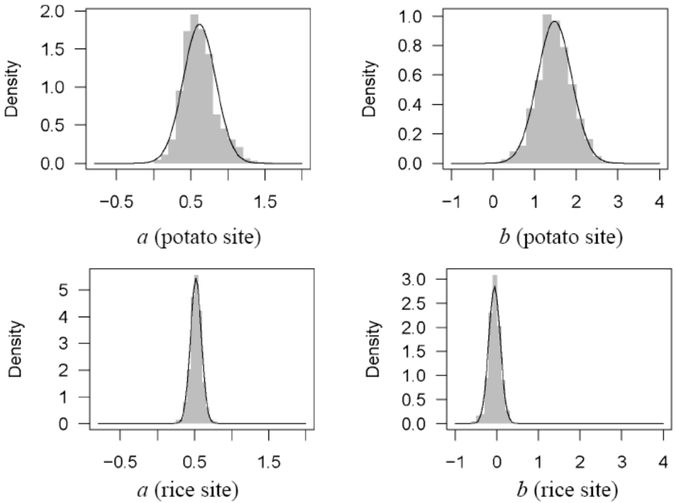
The PM-KP approach was calibrated for the rice field and the potato field individually. This calibration yielded the PM-KP calibration coefficients a and b from the linear regression between rs/ra and r*/ra (Equation (7)) for each site. As it was demonstrated that 20 values of hourly data were sufficient for a reliable calibration in the literature [7,43], this study randomly sampled 40 half-hourly records out of the daytime high quality data (in total, 594 records from the potato site and 361 from the rice site) for calibration. Such calibration procedure was repeated for 1000 runs so as to yield the statistical distributions of a and b, which are shown in Figure 3.
In the case of the potato field, both a and b were found in normal distribution with 0.63 ± 0.21 (mean ± standard deviation) and 1.47 ± 0.42, respectively (Figure 3 upper panel). In the case of the rice field, a showed a normal distribution with 0.52 ± 0.08, and b with −0.06 ± 0.14 (Figure 3 lower panel). The peaks in a and b distributions for the rice site were much more narrow than those for the potato field. The range of both coefficients for the rice site was approximately one-third of those for the potato field.
The sensitivity of the PM-KP model performance is illustrated in Figure 4 by introducing systematic and random errors into a and b. In case of both sites, positive systematic errors for a and b resulted in the increase in ET overestimation (Figure 4A,C). The PM-KP model was as sensitive to a (~2.8% BIASr per systematic error ratio) as to b (~3.0% BIASr per systematic error ratio) for the rice site, and slightly more sensitive to b (~7.6% BIASr per systematic error ratio) than to a (~5.4% BIASr per error ratio) for the potato site. The PM-KP model was nearly twice as sensitive to systematic errors in a and b for the potato field as for the rice field. Random errors (Figure 4B,D) showed less effect to the PM-KP model performance in comparison with systematic errors. Only ~1.9% SEEr per random error ratio in both a and b was found for the rice field, and 3.4% and 4.0% SEEr per random error ratio in a and b, respectively, for the potato field.
3.4. Optimization of PM-FAO Approach
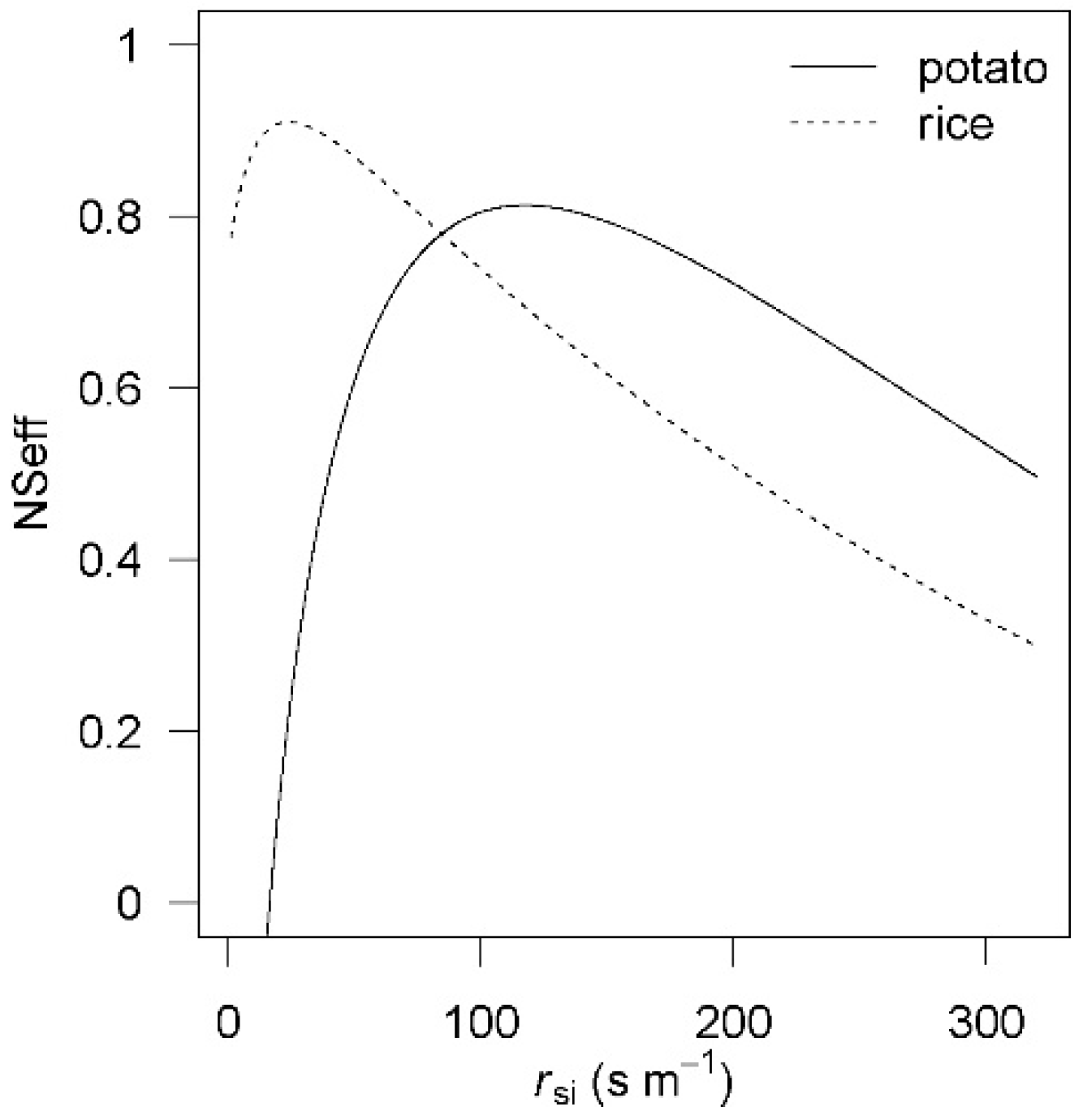
In order to evaluate the performance of the PM-KP approach, the PM-FAO approach was used as a reference for comparison, which was performed with a range of rsi from 0 to 320 s m−1 [44] for both sites (Figure 5). The model efficiency coefficient was obviously changed with the varied value of rsi. For the potato site, the model efficiency coefficient showed a peak value of NSeff = 0.81 at rsi = 117 s m−1 (Figure 5 solid line). Either an increase or decrease of rsi resulted in a sharp decrease in NSeff = 0.6 at rsi = 320 s m−1 or NSeff < 0 at rsi < 20 s m−1. When using the literature values of rsi between 70 and 80 s m−1 [4], NSeff ranged from 0.72 to 0.77, therefore rsi = 117 s m−1 was used as an optimal estimation for the potato site in this study. If compared with using rsi = 75 s m−1 (the medium of the literature values [4]) which resulted in NSeff = 0.75 and regression slope (QEPM-FAO against QEEBC-HB) of 1.06 (n = 1061), the model performance was slightly improved by using rsi = 117 s m−1, with a smaller regression slope of 0.94. The decline of the slope was due to the larger value of rsi, resulting in an increase of the denominator of the PM function and consequently the decrease of the simulated QE.
For the rice site, the pattern of the sensitivity test showed an optimal rsi of 38 s m−1 with NSeff = 0.91 (Figure 5 dotted line) and regression slope (QEPM-FAO against QEEBC-HB) of 0.96 (n = 847). This optimal value of rsi was much smaller than the typical range of rsi in the literature (e.g., [4]) and resulted in better model performance than using the medium of literature value of rsi = 75 s m−1 which resulted in NSeff = 0.80 and regression slope of 0.80. The values of the slope lower than unity indicated that the PM-FAO approach had a tendency to underestimate QE for the rice field in this study, especially in the case of large values of QE.
The optimal site-specific values of rsi were used to estimate ET as a comparison so as to evaluate the performance of PM-KP approach in the subsequent sections.
3.5. Performance of PM-KP Approach
The performance of the PM-KP approach was evaluated with the mean values of a and b of this study, which was described in Section 3.3. ET estimated by PM-KP using a = 0.63 and b = 1.47 gave NSeff = 0.70 and the regression slope (simulation against observation) of 0.91 (n = 594) for the potato site, and a = 0.52 and b = −0.06 gave NSeff = 0.94 and the regression slope of 0.97 (n = 361) for the rice site over the entire growing seasons. Generally speaking, the PM-KP approach performed less effectively for the potato field where ET was underestimated, while better than the PM-FAO approach for the rice field.
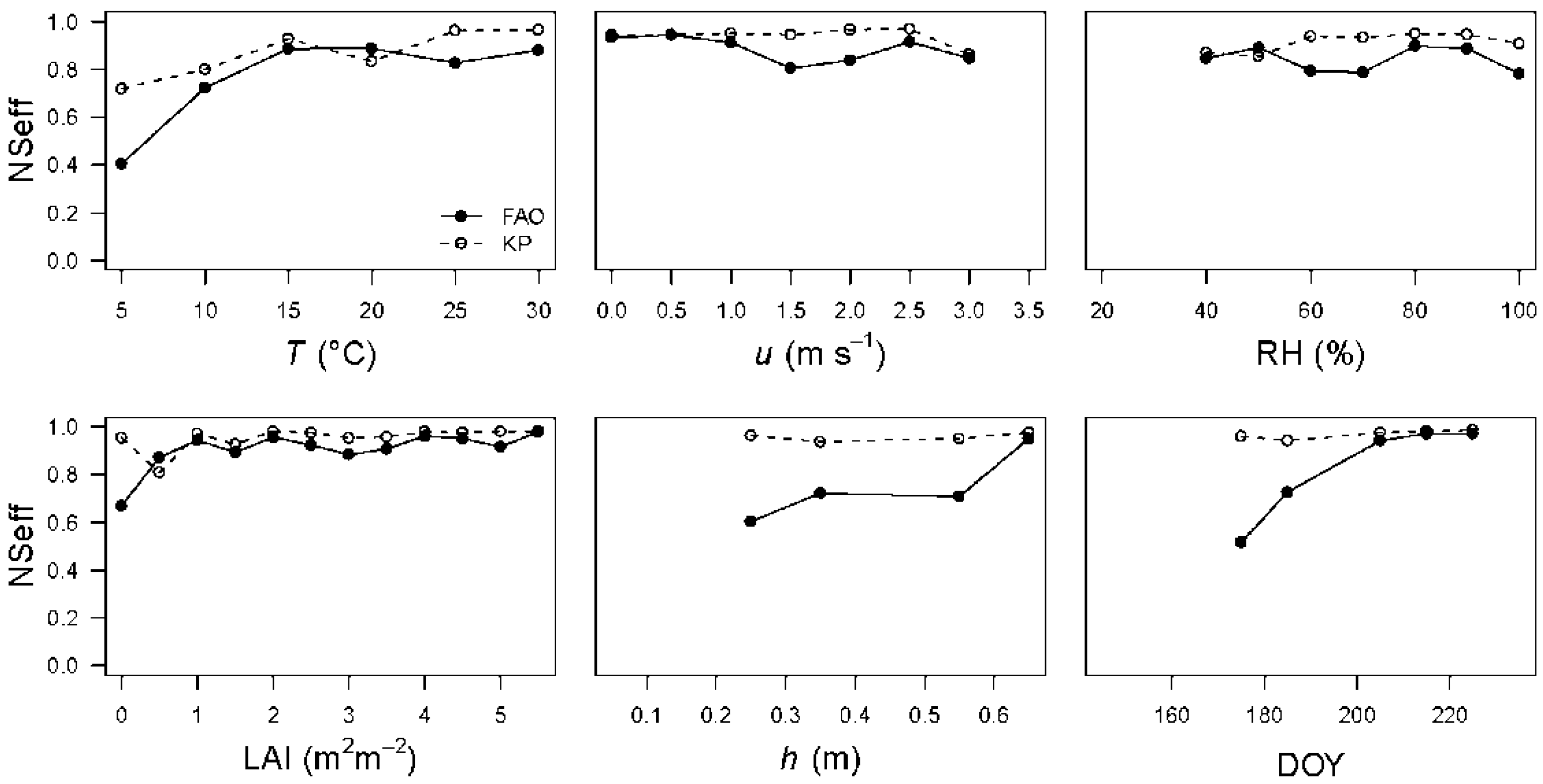
The dependence of the PM-KP model (as well as PM-FAO model) performance on multiple variables was studied by classifying the dataset into groups according to a given interval window of each independent variable (Figure 6 and Figure 7). The interval was set as ±2.5 °C for T, ±0.25 m s−1 for u, ±5% for RH, ±0.25 m2 m−2 for LAI, ±0.05 m for h, and ±5 days for day of the year (DOY). An individual NSeff within each interval window was obtained from the QEPM-KP, QEPM-FAO, and QEEBC-HB values which fell in the given interval window. For instance, NSeff at T = 10 °C displayed in Figure 6 was calculated from those QEPM-FAO and QEEBC-HB values when T ranged between 7.5 and 12.5 °C.
The dependence of model performance on the environment and vegetation variables showed different patterns for the potato site (Figure 6). Both models performed consistently well across the entire ranges of T and u, although with high NSeff > 0.7 at low wind speed and a slight decrease in NSeff when u > 2.0 m s−1. In contrast, the performances of both models showed greater variation with humidity. The model efficiency was very low when the air was dry. Good performances of both models were achieved at high relative humidity (RH > 50%), well developed vegetation (LAI > 1.5 m2 m−2), and tall plant height (h > 0.3 m), with NSeff > 0.8. Actually, these humid conditions coincided with fully developed vegetation from mid-June to July (DOY 170 to 210), resulting in good performance of the models for the potato field in the summer monsoon. The performance of the PM-KP approach for poorly developed vegetation surface (LAI < 1.5 m2 m−2) and short plant (h < 0.3 m) in August (DOY > 210) was better than that of the PM-FAO approach.
In case of the rice field, the dependences of the performances of both the PM-KP approach and the PM-FAO approach on multiple variables are shown in Figure 7. The model efficiency of the PM-KP approach was consistently good across the range of all the studied independent variables, while the model performance of the PM-FAO approach showed large variation. The PM-KP model performed much better than the PM-FAO model at low air temperature (T < 10 °C) or less developed vegetation (LAI > 0.5 m2 m−2, h > 0.6 m). This was because low temperature was only observed in the early morning at the early growing stage of rice, which coincided with the occurrence of poorly developed vegetation, and small QE. Windy conditions with u > 1.5 m s−1 resulted in a better simulation of the PM-KP model than the PM-FAO model, because QE is expected to be enhanced under windy conditions on sunny days in summer, but this effect is insufficiently represented by the PM-FAO approach with the dependence of rs only on LAI [45]. The open standing water, as an evident source of evaporation in the rice field, is apparently unrelated to stomata.
4. Discussion
The PM-KP calibration coefficients a and b have been published for a variety of crops in the literature (Table 1), while their distributions as well as the effects of their errors have not been reported as far as we know. Although the ranges of LAI and crop heights in this study were much wider than other work, the values of a and b were comparable with published values. Particularly, the error in ET estimation resulting from the random sampling of the data for the rice field was much smaller and therefore the calibration was more stable than for the potato field. Thus, one random sample with a limited number of observation records, e.g., 20 samples proposed in the literature [7,43], could be sufficient to parameterize a and b for the rice field even throughout the entire crop growing seasons, but could yield a large deviation in a and b and significant error in ET estimation for the potato field. This was probably due to the seasonally changing water-stress and vegetation conditions in the non-irrigated potato field where plant transpiration played a key role in ET in the pre- and post-monsoon seasons.
Katerji et al. [14] argued that the oversimplified assumption in the PM-FAO approach which ignores the effect of meteorological variables on stomatal resistance could be an important source of uncertainties in ET estimation. The limitation of the PM-FAO approach for the rice field in this study was possibly because Equation (6) yielded too large values of rs when LAI was very small, whereas the flooded rice field for small LAI was almost an open water surface and the actual rs was close to zero, thus rs was much overestimated by the PM-FAO approach. The PM-KP approach had the advantage because it was consistent with the fact that QE is dominantly controlled by the meteorological factors rather than LAI in well-irrigated crops [45]. It was reported that the calibration of the FAO-KP approach is species-specific [48] and the coefficient a and b need calibration for (1) well-watered crops in the development growth stage; (2) well-watered crops in the senescence stage; and (3) water-stressed crops during the development stage [8,14,43]. On one hand, our study on the distribution of a and b and the error analysis agrees well with these situations. On the other hand, a and b are not sensitive to the variety of the vegetation development in the rice field, and can be considered to be constant for the entire growing season of rice.
The research sites in this study were highly influenced by East Asian monsoon. It was reported that the observed VPD is below the plant physiological threshold (10 hPa) during most of the time of the growing season of rice owing to the permanently flooded terraces with the contribution of intensive precipitation in summer monsoon in the research region [28]. However, the model performance of the PM-KP approach was weak for dry air conditions in the potato field, possibly because of the regulation of leaf water potential by stomata. It was reported that 1/rs decreases linearly with log(VPD) for plant species and stomatal sensitivity is proportional to the magnitude of 1/rs at low VPD (≤10 hPa) [49], which was later demonstrated to be consistent with the linear model presented by [50]. High temperature as well as high VPD in the afternoon in dry pre-monsoon season leads to a high evapotranspiration rate and then to a stomatal closure for potato plants in the research region [28]. This regulation could result in a deviation of rs from the estimation by Equations (6) and (7), and consequently the poor efficiency of both the PM-KP approach and the PM-FAO approach in the case of the dry air. In the future, the Asian summer monsoon is predicted to be extended and rainfall to be increased in the research region [51]. Therefore, it could be expected that the rain-fed croplands like potato fields would be better watered, and the VPD influence on stomatal closure would be weakened, and the PM-KP could perform better for this region.
5. Conclusions
The stomatal resistance played a very important role in ET estimation by the PM model for typical flooded and non-irrigated East Asian croplands. This study on the PM-KP approach showed for the first time the statistical distributions of the PM-KP coefficients a and b. Furthermore, these distributions indicated that the calibration of the PM-KP model for the rice field was more stable than for the potato field. A limited number of randomly sampled observation records in the entire crop growing seasons should be satisfactory to parameterize a and b for the rice field, but could yield a large uncertainty in ET estimation for the potato field. The analysis of systematic and random errors in a and b demonstrated that errors in the calibration coefficients for the potato site had more of an effect on ET estimation for the potato field than the rice field. Therefore, it is suggested that a and b should be derived via the statistic distribution for the sake of better model performance. Compared with the PM-FAO approach, the PM-KP approach performed generally better for the rice field but worse for the potato field, probably because the PM-KP approach is more effective for evaporation-dominated surfaces and the PM-FAO approach has the advantage for transpiration-dominated surfaces.
In conclusion, this study makes it possible to choose the optimized approach for ET estimation in East Asia, where agriculture is highly influenced by the summer monsoon. The PM-KP approach would be a better alternative than the PM-FAO approach for estimating ET over croplands such as flooded rice fields where evaporation acts as the major share of ET. On the other hand, the PM-KP approach would be an acceptable alternative for rain-fed croplands when the soil is well watered and the air is humid during the summer monsoon. Further studies are encouraged to discover the detailed effect of soil water stress on the performance of the PM-KP model.
Acknowledgments
We deeply thank Thomas Foken for his helpful comments. We also thank John Tenhunen for the major support without which this work would not be possible. We appreciate the help given by the colleagues of the Department of Micrometeorology and Department of Plant Ecology, University of Bayreuth. This work was supported by the German Research Foundation [GRK 1565/1] and the open access funding of University of Bayreuth.
Author Contributions
Peng Zhao and Johannes Lüers designed and performed the experiments; Peng Zhao analyzed the data and wrote the paper under Johannes Lüers’s supervision.
Conflicts of Interest
The authors declare no conflict of interest.
References
- Kang, S.; Su, X.; Tong, L.; Zhang, J.; Zhang, L. A warning from an ancient oasis: Intensive human activities are leading to potential ecological and social catastrophe. Int. J. Sustain. Dev. World Ecol. 2008, 15, 440–447. [Google Scholar] [CrossRef]
- Rana, G.; Katerji, N. Measurement and estimation of actual evapotranspiration in the field under Mediterranean climate: A review. Eur. J. Agron. 2000, 13, 125–153. [Google Scholar] [CrossRef]
- Wang, K.; Dickinson, R.E. A review of global terrestrial evapotranspiration: Observation, modeling, climatology, and climatic variability. Rev. Geophys. 2012, 50, RG2005. [Google Scholar] [CrossRef]
- Allen, R. Penman-Monteith equation. In Encyclopedia of Soils in the Environment; Hillel, D., Ed.; Elsevier: Oxford, UK, 2005; pp. 180–188. [Google Scholar]
- Allen, R.G.; Pereira, L.S.; Raes, D.; Smith, M. Crop Evapotranspiration: Guidelines for Computing Crop Water requireMents. FAO Irrigation and Drainage Paper 56; Food and Agriculture Organisation of the United Nations: Rome, Italy, 1998. [Google Scholar]
- Cleugh, H.A.; Leuning, R.; Mu, Q.; Running, S.W. Regional evaporation estimates from flux tower and MODIS satellite data. Remote Sens. Environ. 2007, 106, 285–304. [Google Scholar] [CrossRef]
- Katerji, N.; Rana, G. Modelling evapotranspiration of six irrigated crops under Mediterranean climate conditions. Agric. For. Meteorol. 2006, 138, 142–155. [Google Scholar] [CrossRef]
- Katerji, N.; Perrier, A. Modélisation de l’évapotranspiration réelle ETR d’une parcelle de luzerne: Rôle d’un coefficient cultural. Agronomie 1983, 3, 513–521. [Google Scholar] [CrossRef]
- Alves, I.; Pereira, L.S. Modelling surface resistance from climatic variables? Agric. Water Manag. 2000, 42, 371–385. [Google Scholar] [CrossRef]
- Rana, G.; Katerji, N.; Lorenzi, F. de Measurement and modelling of evapotranspiration of irrigated citrus orchard under Mediterranean conditions. Agric. For. Meteorol. 2005, 128, 199–209. [Google Scholar] [CrossRef]
- Rana, G.; Katerji, N.; Mastrorilli, M.; El Moujabber, M. A model for predicting actual evapotranspiration under soil water stress in a Mediterranean region. Theor. Appl. Climatol. 1997, 56, 45–55. [Google Scholar] [CrossRef]
- Rana, G.; Katerji, N.; Perniola, M. Evapotranspiration of sweet sorghum: A general model and multilocal validity in semiarid environmental conditions. Water Resour. Res. 2001, 37, 3237–3246. [Google Scholar] [CrossRef]
- Steduto, P.; Todorovic, M.; Caliandro, A.; Rubino, P. Daily reference evapotranspiration estimates by the Penman-Monteith equation in Southern Italy. Constant vs. variable canopy resistance. Theor. Appl. Climatol. 2003, 74, 217–225. [Google Scholar] [CrossRef]
- Katerji, N.; Rana, G. FAO-56 methodology for determining water requirement of irrigated crops: Critical examination of the concepts, alternative proposals and validation in Mediterranean region. Theor. Appl. Climatol. 2014, 116, 515–536. [Google Scholar] [CrossRef]
- Asian Development Bank; International Food Policy Research Institute. Building Climate Resilience in the Agriculture Sector of Asia and the Pacific; Asian Development Bank: Mandaluyong, Philippines, 2009. [Google Scholar]
- Cabangon, R.; Tuong, T.; Tiak, E.; Abdullah, N. bin Increasing water productivity in rice cultivation: Impact of large-scale adoption of direct seeding in the Muda irrigation system. In Direct Seeding in Asian Rice Systems: Strategic Research Issues and Opportunities, Proceedings of an International Workshop on Direct Seeding in Asia, Bangkok, Thailand, 25–28 January 2000. pp. 299–313.
- Fabeiro, C.; de Santa Olalla, F.M.; De Juan, J. Yield and size of deficit irrigated potatoes. Agric. Water Manag. 2001, 48, 255–266. [Google Scholar] [CrossRef]
- Jo, K.; Lee, H.; Park, J.; Owen, J.S. Effects of Monsoon Rainfalls on Surface Water Quality in a Mountainous Watershed under Mixed Land Use. Korean J. Agric. For. Meteorol. 2010, 12, 197–206. [Google Scholar] [CrossRef]
- Ruidisch, M.; Kettering, J.; Arnhold, S.; Huwe, B. Modeling water flow in a plastic mulched ridge cultivation system on hillslopes affected by South Korean summer monsoon. Agric. Water Manag. 2013, 116, 204–217. [Google Scholar] [CrossRef]
- Foken, T. Micrometeorology; Springer: Berlin, Germany, 2008. [Google Scholar]
- Mauder, M.; Foken, T. Documentation and Instruction Manual of the Eddy Covariance Software Package TK3; University of Bayreuth, Department of Micrometeorology: Bayreuth, Germany, 2011. [Google Scholar]
- Foken, T.; Leuning, R.; Oncley, S.; Mauder, M.; Aubinet, M. Corrections and Data Quality Control. In Eddy Covariance; Aubinet, M., Vesala, T., Papale, D., Eds.; Springer Atmospheric Sciences; Springer: Dordrecht, The Netherlands, 2012; pp. 85–131. [Google Scholar]
- Foken, T.; Wichura, B. Tools for quality assessment of surface-based flux measurements. Agric. For. Meteorol. 1996, 78, 83–105. [Google Scholar] [CrossRef]
- Lüers, J.; Detsch, F.; Zhao, P. Application of a Multi-Step Error Filter for Post-Processing Atmospheric Flux and Meteorological Basic Data; University of Bayreuth, Department of Micrometeorology: Bayreuth, Germany, 2014. [Google Scholar]
- Eigenmann, R.; Kalthoff, N.; Foken, T.; Dorninger, M.; Kohler, M.; Legain, D.; Pigeon, G.; Piguet, B.; Schüttemeyer, D.; Traulle, O. Surface energy balance and turbulence network during the Convective and Orographically-induced Precipitation Study (COPS). Q. J. R. Meteorol. Soc. 2011, 137, 57–69. [Google Scholar] [CrossRef]
- Göckede, M.; Foken, T.; Aubinet, M.; Aurela, M.; Banza, J.; Bernhofer, C.; Bonnefond, J.M.; Brunet, Y.; Carrara, A.; Clement, R.; et al. Quality control of CarboEurope flux data–Part 1: Coupling footprint analyses with flux data quality assessment to evaluate sites in forest ecosystems. Biogeosciences 2008, 5, 433–450. [Google Scholar] [CrossRef]
- Zhao, P.; Lüers, J.; Olesch, J.; Foken, T. Complex TERRain and ECOlogical Heterogeneity (TERRECO): WP 1–02: Spatial Assessment of Atmosphere-Ecosystem Exchanges via Micrometeorological Measurements, Footprint Modeling and Mesoscale Simulations; Documentation of the Observation Period May 12th to Nov. 8th, 2010, Haean, South Korea; University of Bayreuth, Department of Micrometeorology: Bayreuth, Germany, 2011. [Google Scholar]
- Zhao, P.; Lüers, J. Improved data gap-filling schemes for estimation of net ecosystem exchange in typical East-Asian croplands. Sci. China Earth Sci. 2016, 59, 1652–1664. [Google Scholar] [CrossRef]
- Liebethal, C.; Foken, T. Evaluation of six parameterization approaches for the ground heat flux. Theor. Appl. Climatol. 2007, 88, 43–56. [Google Scholar] [CrossRef]
- Oncley, S.P.; Foken, T.; Vogt, R.; Kohsiek, W.; DeBruin, H.A.R.; Bernhofer, C.; Christen, A.; Gorsel, E.; Grantz, D.; Feigenwinter, C.; et al. The energy balance experiment EBEX-2000. Part I: Overview and energy balance. Bound.-Layer Meteorol. 2007, 123, 1–28. [Google Scholar] [CrossRef]
- Foken, T. The energy balance closure problem: An overview. Ecol. Appl. 2008, 18, 1351–1367. [Google Scholar] [CrossRef] [PubMed]
- Foken, T.; Mauder, M.; Liebethal, C.; Wimmer, F.; Beyrich, F.; Leps, J.P.; Raasch, S.; DeBruin, H.A.R.; Meijninger, W.M.L.; Bange, J. Energy balance closure for the LITFASS-2003 experiment. Theor. Appl. Climatol. 2010, 101, 149–160. [Google Scholar] [CrossRef]
- Kanda, M.; Inagaki, A.; Letzel, M.O.; Raasch, S.; Watanabe, T. LES study of the energy imbalance problem with eddy covariance fluxes. Bound.-Layer Meteorol. 2004, 110, 381–404. [Google Scholar] [CrossRef]
- Charuchittipan, D.; Babel, W.; Mauder, M.; Beyich, F.; Leps, J.P.; Foken, T. Extension of the averaging time of the eddy-covariance measurement and its effect on the energy balance closure. Bound.-Layer Meteorol. 2017. accepted. [Google Scholar] [CrossRef]
- Monteith, J. Evaporation and the environment. In Symposium of the Society for Experimental Biology, The State and Movement of Water in Living Organisms; Cambridge University Press: Cambridge, UK, 1965; Volume 19, pp. 205–234. [Google Scholar]
- Penman, H.L. Natural evaporation from open water, bare soil and grass. Proc. R. Soc. Lond. Ser. A Math. Phys. Sci. 1948, 193, 120–145. [Google Scholar] [CrossRef]
- Beven, K. A sensitivity analysis of the Penman-Monteith actual evapotranspiration estimates. J. Hydrol. 1979, 44, 169–190. [Google Scholar] [CrossRef]
- McCuen, R.H. A sensitivity and error analysis of procedures used for estimating evaporation. J. Am. Water Res. Assoc. 1974, 10, 486–497. [Google Scholar] [CrossRef]
- Nash, J.E.; Sutcliffe, J.V. River flow forecasting through conceptual models part I—A discussion of principles. J. Hydrol. 1970, 10, 282–290. [Google Scholar] [CrossRef]
- Estévez, J.; Gavilán, P.; Berengena, J. Sensitivity analysis of a Penman–Monteith type equation to estimate reference evapotranspiration in southern Spain. Hydrol. Process. 2009, 23, 3342–3353. [Google Scholar] [CrossRef]
- Ley, T.; Hill, R.; Jensen, D. Errors in Penman-Wright alfalfa reference evapotranspiration estimates: I. Model sensitivity analyses. Trans. ASAE 1994, 37, 1853–1861. [Google Scholar] [CrossRef]
- Meyer, S.J.; Hubbard, K.G.; Wilhite, D.A. Estimating potential evapotranspiration: The effect of random and systematic errors. Agric. For. Meteorol. 1989, 46, 285–296. [Google Scholar] [CrossRef]
- Katerji, N.; Rana, G.; Fahed, S. Parameterizing canopy resistance using mechanistic and semi-empirical estimates of hourly evapotranspiration: Critical evaluation for irrigated crops in the Mediterranean. Hydrol. Process. 2011, 25, 117–129. [Google Scholar] [CrossRef]
- Garratt, J. The Atmospheric Boundary Layer; Cambridge University Press: Cambridge, UK, 1992. [Google Scholar]
- Perez, P.J.; Lecina, S.; Castellvi, F.; Martínez-Cob, A.; Villalobos, F. A simple parameterization of bulk canopy resistance from climatic variables for estimating hourly evapotranspiration. Hydrol. Process. 2006, 20, 515–532. [Google Scholar] [CrossRef]
- Rana, G.; Katerji, N.; Mastrorilli, M.; El Moujabber, M.; Brisson, N. Validation of a model of actual evapotranspiration for water stressed soybeans. Agric. For. Meteorol. 1997, 86, 215–224. [Google Scholar] [CrossRef]
- Rana, G.; Katerji, N.; Ferrara, R.M.; Martinelli, N. An operational model to estimate hourly and daily crop evapotranspiration in hilly terrain: Validation on wheat and oat crops. Theor. Appl. Climatol. 2011, 103, 413–426. [Google Scholar] [CrossRef]
- Katerji, N.; Rana, G. Crop Evapotranspiration Measurements and Estimation in the Mediterranean Region; French National Institute for Agricultural Research (INRA)–Agricultural Research Council (CRA): Bari, Italy, 2008. [Google Scholar]
- Oren, R.; Sperry, J.; Katul, G.; Pataki, D.; Ewers, B.; Phillips, N.; Schäfer, K. Survey and synthesis of intra-and interspecific variation in stomatal sensitivity to vapour pressure deficit. Plant Cell Environ. 1999, 22, 1515–1526. [Google Scholar] [CrossRef]
- Katul, G.; Palmroth, S.; Oren, R. Leaf stomatal responses to vapour pressure deficit under current and CO2-enriched atmosphere explained by the economics of gas exchange. Plant Cell Environ. 2009, 32, 968–979. [Google Scholar] [CrossRef] [PubMed]
- Yun, K.S.; Shin, S.H.; Ha, K.J.; Kitoh, A.; Kusunoki, S. East Asian precipitation change in the global warming climate simulated by a 20-km mesh AGCM. Asia-Pac. J. Atmos. Sci. 2008, 44, 233–247. [Google Scholar]
Figure 1.
Meteorological conditions and vegetation development at the research sites, including daily mean air temperature (T, solid line in A), daily mean relative humidity (RH, dashed line in A), daily sum precipitation (P, solid line in B), daily mean solar radiation (Rg, dashed line in B), and leaf area index (LAI, dashed line representing potato and solid line representing rice in C with standard deviations as error bars), and plant height (dashed line representing potato and solid line representing rice in D).
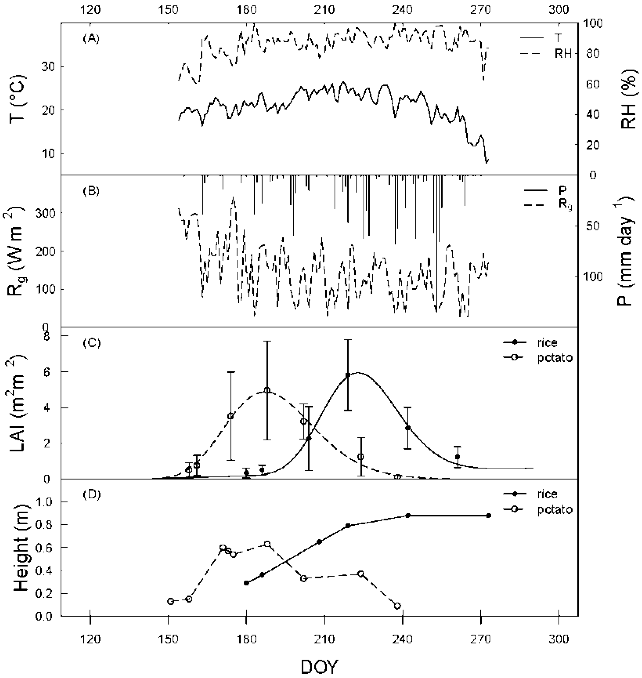
Figure 2.
Diurnal (A,B) and seasonal (C,D) patterns of Penman-Monteith model sensitivity coefficients for available energy (closed circle), vapor pressure deficit (VPD, open circle), aerodynamic resistance (cross), and stomatal resistance (closed square) in the rice field (A,C) and in the potato field (B,D).
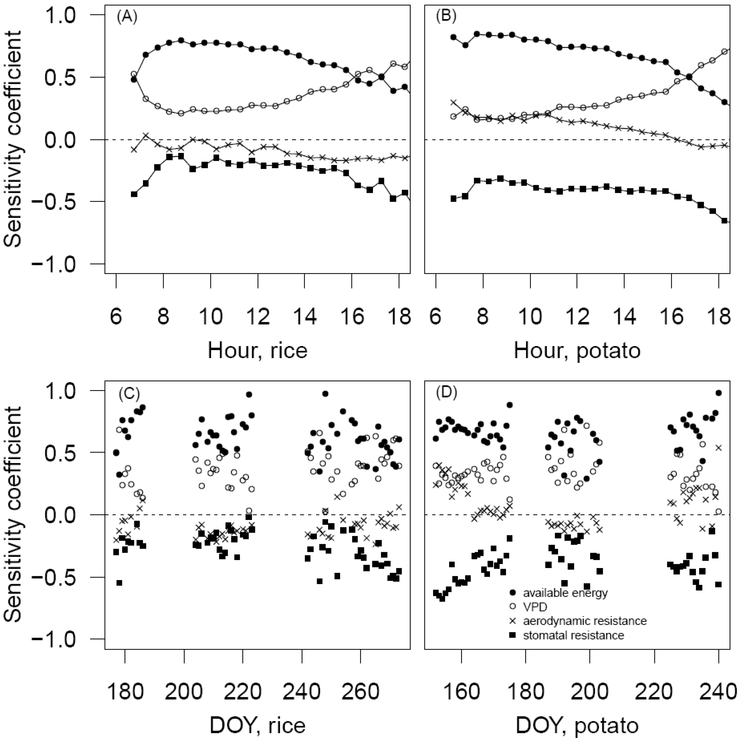
Figure 3.
Statistical distribution of the regression coefficients a and b of the Penman-Monteith-Katerji-Perrier (PM-KP) approach for the potato site (upper) and the rice site (lower).
Figure 3.
Statistical distribution of the regression coefficients a and b of the Penman-Monteith-Katerji-Perrier (PM-KP) approach for the potato site (upper) and the rice site (lower).

Figure 4.
Sensitivity of PM-KP modelled evapotranspiration to systematic errors (A,C) and random errors (B,D) in PM-KP coefficients a (solid line with closed circle) and b (dotted line with open circle) for the potato site (A,B) and the rice site (C,D).
Figure 4.
Sensitivity of PM-KP modelled evapotranspiration to systematic errors (A,C) and random errors (B,D) in PM-KP coefficients a (solid line with closed circle) and b (dotted line with open circle) for the potato site (A,B) and the rice site (C,D).
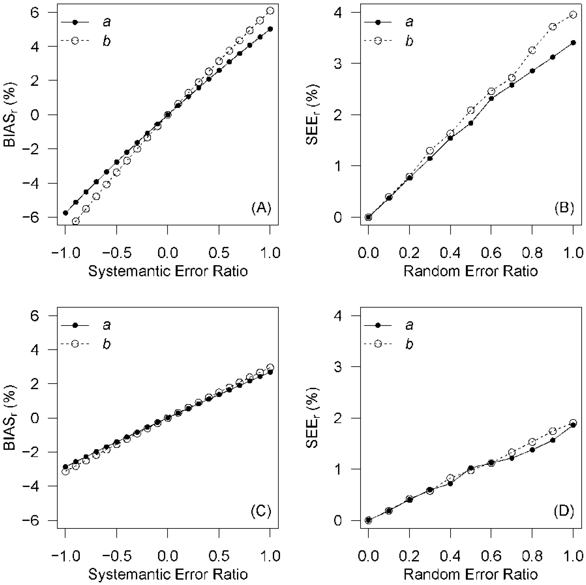
Figure 5.
Nash-Sutcliffe model efficiency coefficient (NSeff) of PM-FAO (Penman-Monteith-Food and Agriculture Organization) modelled QE to modifications in rsi for the potato field (solid line) and rice field (dotted line).
Figure 5.
Nash-Sutcliffe model efficiency coefficient (NSeff) of PM-FAO (Penman-Monteith-Food and Agriculture Organization) modelled QE to modifications in rsi for the potato field (solid line) and rice field (dotted line).

Figure 6.
Nash-Sutcliffe model efficiency coefficient (NSeff) of simulated evapotranspiration by PM-FAO approach (solid line with closed circle) and PM-KP approach (dash line with open circle) against air temperature (T), wind speed (u), relative humidity (RH), leaf area index (LAI), plant height (h), and day of the year (DOY), for the potato field.
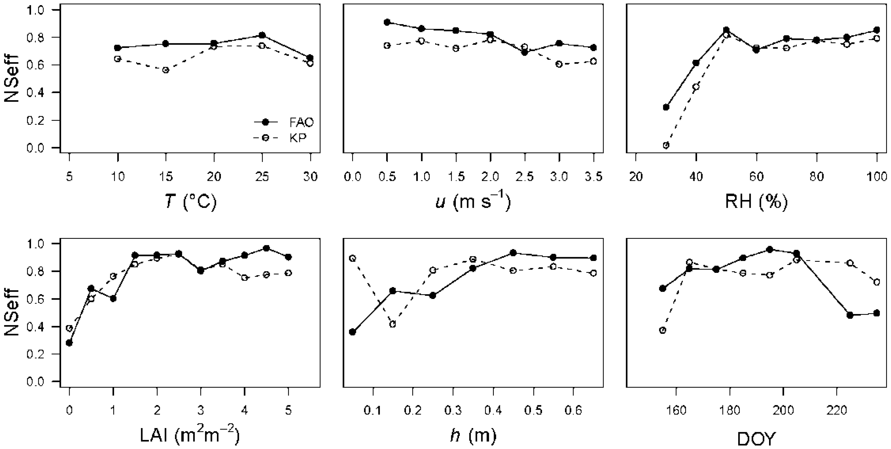
Figure 7.
Nash-Sutcliffe model efficiency coefficient (NSeff) of simulated evapotranspiration by the PM-FAO approach (solid line with closed circle) and the PM-KP approach (dash line with open circle) against air temperature (T), wind speed (u), relative humidity (RH), leaf area index (LAI), plant height (h), and day of the year (DOY), for the rice field.


Table 1.
Calibration coefficients of the PM-KP model.
| Species | LAI (m2 m−2) | Crop Height (m) | a | b | References |
|---|---|---|---|---|---|
| Alfalfa | NA | NA | 0.31 | 0.25 | [8] |
| Clementine | 2.1–2.6 | 4.08 ± 0.23 | 0.23 | 0.0042 | [10] |
| Grain sorghum | NA | NA | 0.56 ± 0.12 | 0.6 ± 0.7 | [46] |
| Grass | 2–2.5 | 0.1 | 0.16 ± 0.02 | 0 ± 0.02 | [43,46] |
| Lettuce | NA | 0.15–0.20 | 0.73 | −0.58 | [9,14] |
| Oats | NA | NA | 0.88 | 3.39 | [47] |
| Soybean | 2–4 | 0.8 | 0.95 | 1.55 | [43] |
| Sunflower | NA | NA | 0.45 ± 0.06 | 0.2 ± 0.35 | [46] |
| Sweet sorghum | 3–6.4 | 2 | 0.84 | 1.00 | [7,43] |
| Tomato | 0.5–3.8 | 0.7 | 0.54 ± 0.1 | 2.4 ± 1.2 | [7] |
| Vineyard | 2–2.8 | 2.2 | 0.91 | 0.45 | [43] |
| Wheat | 2.5–3.1 | 1 | 0.96 | 4.24 | [47] |
| Rice | 0–5.8 | 0.3–0.9 | 0.52 ± 0.08 | −0.06 ± 0.14 | this study |
| Potato | 0–4 | 0–0.6 | 0.63 ± 0.21 | 1.47 ± 0.42 | this study |
© 2017 by the authors. Licensee MDPI, Basel, Switzerland. This article is an open access article distributed under the terms and conditions of the Creative Commons Attribution (CC BY) license (http://creativecommons.org/licenses/by/4.0/).
Share and Cite
MDPI and ACS Style
Zhao, P.; Lüers, J. Parameterization of Evapotranspiration Estimation for Two Typical East Asian Crops. Atmosphere 2017, 8, 111. https://doi.org/10.3390/atmos8060111
AMA Style
Zhao P, Lüers J. Parameterization of Evapotranspiration Estimation for Two Typical East Asian Crops. Atmosphere. 2017; 8(6):111. https://doi.org/10.3390/atmos8060111
Chicago/Turabian StyleZhao, Peng, and Johannes Lüers. 2017. "Parameterization of Evapotranspiration Estimation for Two Typical East Asian Crops" Atmosphere 8, no. 6: 111. https://doi.org/10.3390/atmos8060111
Note that from the first issue of 2016, this journal uses article numbers instead of page numbers. See further details here.