Sensitivity Study on High-Resolution WRF Precipitation Forecast for a Heavy Rainfall Event


Weather Information Service Engine, Hankuk University of Foreign Studies, YongIn-si 17035, Korea
*
Author to whom correspondence should be addressed.
Atmosphere 2017, 8(6), 96; https://doi.org/10.3390/atmos8060096
Submission received: 19 April 2017
/
Revised: 15 May 2017
/
Accepted: 23 May 2017
/
Published: 24 May 2017
(This article belongs to the Special Issue WRF Simulations at the Mesoscale: From the Microscale to Macroscale)
Abstract
:A high-resolution Weather Research and Forecasting (WRF) model for a heavy rainfall case is configured and the performance of the precipitation forecasting is evaluated. Sensitivity tests were carried out by changing the model configuration, such as domain size, sea surface temperature (SST) data, initial conditions, and lead time. The numerical model employs one-way nesting with horizontal resolutions of 5 km and 1 km for the outer and inner domains, respectively. The model domain includes the capital city of Seoul and its suburban megacities in South Korea. The model performance is evaluated via statistical analysis using the correlation coefficient, deviation, and root mean squared error by comparing with observational data including, but not limited to, those from ground-based instruments. The sensitivity analysis conducted here suggests that SST data show negligible influence for a short range forecasting model, the data assimilated initial conditions show the more effective results rather than the non-assimilated high resolution initial conditions, and for a given domain size of the forecasting model, an appropriate outer domain size and lead time of <6 h for a 1-km high-resolution domain should be taken into consideration when optimizing the WRF configuration for regional torrential rainfall events around Seoul and its suburban area, Korea.
1. Introduction
Over the last several decades, dangerous weather events such as severe rain, heavy snow, drought, and heat wave caused by climate change have been concentrated over densely populated urban and industrial areas. In particular, in Korea, localized torrential rainfall has caused flash floods and mountain landslides, sometimes resulting in heavy casualties and property loss [1]. To prevent such substantial damage, it is important to predict heavy rainfall over densely populated and industrial areas within a short time range.
In this study, the forecasting is focused on the local atmospheric circulation over the complex megacities in Korea. The 1-km resolution forecasting model has a highly resolved model configuration, and its forecasting skills are sensitive to the input data and configuration. Thus, such information plays an important role in improving the skills of the forecasting model for local atmospheric circulation. Sensitivity analyses of model performances have traditionally focused on model physics, initial conditions, and sea surface temperature (SST). The analyses associated with outer domain size and lead time are rarely considered. The objective of this study is thus to investigate the ability of a forecasting model, representing complex megacities and large urban areas, for heavy rainfall events by examining the effects of model configuration and various input data sources, such as outer domain size, sea surface temperature, initial conditions, and lead-time effect. Although this study does not attempt to reach conclusions for the optimal configuration for all heavy rainfall events, as a pilot study, it identifies the weaknesses and strengths of various model configurations, and provides insight into high resolution model configuration for multi-hazard impact-based forecasting and warning services.
Three-dimensional primitive-equation atmosphere circulation models, such as the Weather Research and Forecasting (WRF) model [2], the Global/Regional Integrated Model System (GRIMs) [3], and others, have been utilized to forecast precipitation events. In addition, high-resolution numerical simulations of local atmospheric flow in regions that include urban areas have begun to provide credible representations of the three-dimensional local atmospheric circulation on horizontal scales of several kilometers [4,5,6,7]. For this study, the WRF model developed at the National Center of Atmospheric Research (NCAR) is utilized. The numerical model has been used for high-resolution configurations to resolve and understand the meteorological challenges faced by complex megacities and large urban areas, which include buildings of various heights, paved streets, and parks [8].
In atmospheric research, there have been few studies on the predictability of heavy rainfall in terms of uncertainties associated with domain size and lead time in high resolution models. Wang et al. [9] examined the sensitivity of heavy precipitation to horizontal resolution, domain size, and rain rate assimilation for case studies using a convection-permitting model. Dravitzki and McGregor [10] investigated heavy rainfall events over the Waikato River Basin of New Zealand generated with higher-resolution WRF, and Goswami et al. [11,12] showed that domain size is as important as grid spacing and initial conditions for heavy rainfall events. Additionally, Li et al. [13] analyzed the influence of horizontal resolution, domain size, and physical parameterization schemes to evaluate an optimized WRF precipitation forecast over a region of complex topography during the flood season. The research-grade and storm-scaled operational Numerical Weather Prediction (NWP) models of the Korea Meteorology Administration (KMA) regularly produce simulations with a horizontal grid spacing as fine as 1 km over the megacity of Seoul and its surrounding cities, and have been used to obtain new insights to develop a high-resolution model configuration based on WRF [14,15].
This paper is organized as follows. Section 2 provides a summary of the default model configuration and the meteorological aspects of a heavy precipitation event and also evaluates the numerical results by comparing with observations. Section 3 describes the design of the sensitivity experiments, documents their results, and provides an overall discussion. Finally, a summary and concluding remarks are provided in Section 4.
2. Model Formulation
2.1. Model Configuration
The Weather Research and Forecasting (WRF) Model developed at NCAR in the United States is a non-hydrostatic, incompressible model that has been used in various research studies [2]. The model configuration used here is the same as that described in [16] with WRF version 3.6.1 representing Seoul and its suburban cities in Korea (Figure 1). That is, the model is configured in the Lambert conformal map projection with the central latitude of 38° N and longitude of 126° E. It uses a one-way nested domain configuration consisting of a 5-km resolution outer domain (Figure 1a) and a 1-km resolution inner domain (Figure 1b), with 332 × 293 and 336 × 286 grid points, respectively. The model configuration for the inner domain uses an ample buffer zone of five grid points and an exponential transition at the border. Fifty vertical levels with a maximum height of 50 hPa are used for both domains. There were 54 Automated Weather Stations (AWS) (Figure 1c, red dots) in the metropolitan area, and observed meteorological values from these stations were used to evaluate the model performance.
The forecasting model terrain has a 1-km horizontal resolution that is smoothed from a 3-s (~90 m) terrain database. We adopted the same configuration for the physical parameterization that is utilized in the Korean Local Analysis and Prediction System (KLAPS) operational model, which is run by the Korea Meteorological Administration (KMA). The KMA performs a very short-range research-graded high-resolution WRF model at 5-km resolution for the outer domain and 1-km resolution for the data assimilated one-way nested inner domain. This study focuses on the same configuration used in the research-graded model.
The physical parameterization included the YonSei University (YSU) scheme for planetary boundary layers (PBL) [17], WRF Double-Moment 6-class (WDM6) microphysics [18], the Unified Noah Land Surface Model [19], and the New Goddard Scheme [20] for longwave and shortwave radiation. Table 1 shows a summary of the default model configuration and physical parameterizations. These options for parameterizations are the same for both the outer and inner domains, except for the cumulus schemes. The initial and boundary conditions for the inner domain are provided by the model results from the outer domain, whose initial and boundary conditions are obtained from the regional 12-km Unified Model (UM) operated by the KMA. The 5-km Operational Sea Surface Temperature and Sea Ice Analysis (OSTIA) sea surface temperature from the Meteorological (MET) office and 100 km soil moisture and soil temperature from the National Center for Environmental Prediction (NCEP) Final Operational Global Analysis Reanalysis Data (NCEP-FNL) were used.
2.2. Heavy Rainfall Event
Generally, rainfall in Korea occurs during the rainy season, from the end of June to the end of July, and is associated with the East Asian Monsoon and typhoons. During the summer season, there is usually a warm and wet air flow with a generally predictable pattern of southwesterly winds off the Yellow Sea, which results in heavy rainfall over Korea. Summer rainfall amounts are more than half the annual precipitation in most regions of South Korea, and an increasing number of extreme events have been related to mesoscale convective systems with the synoptic-scale East Asian Summer Monsoon. Rain systems related to the East Asian Monsoon over the Korean Peninsula are classified into four categories: cloud clusters (47%), convective bands (27%), isolated thunderstorms (12%), and squall lines (7%) [21]. Additionally, synoptic precipitation patterns over a period of 30 years for South Korea have been classified into 10 categories based on surface map analysis [22].
During a rainfall event from 26 July to 28 July 2011, the main characteristics of the development of heavy rainfall were first the favorable synoptic-scale features of relatively heavy rainfall, and then convective systems continuously moved from the Yellow Sea to the region northwest of Seoul (Figure 2). Thus, the moist warm air was transported over the mid-western Korean Peninsula by the southwesterly low-level jets between the flank of the Western Pacific Subtropical High (WPSH), located over the region southeast of Korea and Japan, and a low-pressure trough over north China. The westward movement of the low pressure over north China was blocked by a cutoff blocking high located near the Sea of Okhotsk [23].
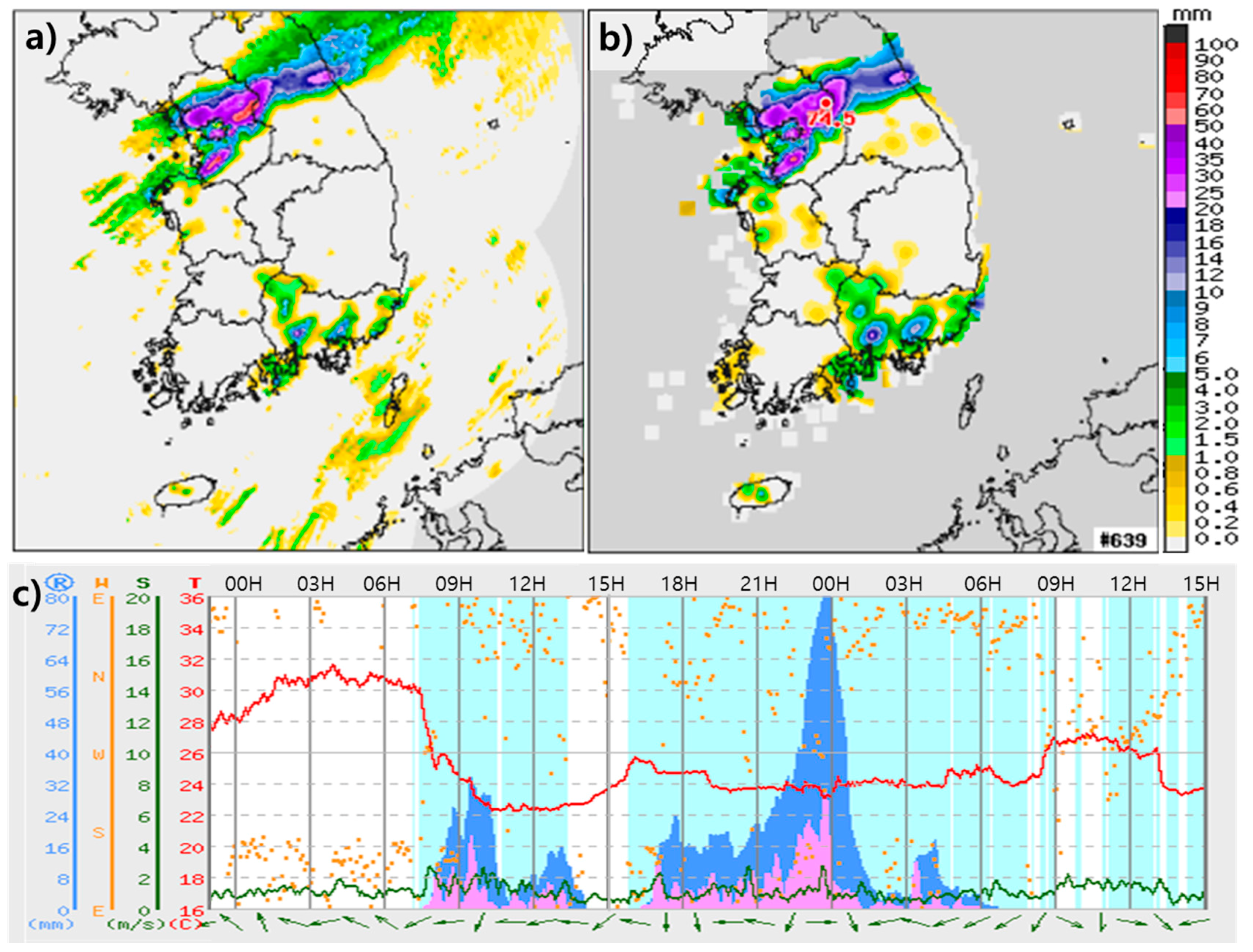
Most of the rainfall was observed during the 24-h period from 1500 UTC 26 July to 1500 UTC 27 July 2011. During this period, rainfall of 110 mm per hour and 300 mm per day over Seoul, Korea, led to landslides and flooding, resulting in human casualties and economic damage. Figure 3a,b shows the one hour accumulated rainfall analysis fields from Radar and AWSs, provided by the KMA. Note that the AWS data values were remapped using area-weighted averages onto the grid resolution. Hourly accumulated rainfall reached its local maxima of 74.2 mm/h over southeastern Seoul. Then, the rainfall system moved toward the northwest from Seoul, and new convective systems continuously developed from the west coast to Seoul. Figure 3c shows the time series of meteorological values from one AWS, which represents the meteorological values for Seoul (white dot in Figure 1b). The accumulated precipitation, in the meteogram, indicated with blue-color shading, also shows the second convective system that continuously developed from the west coast, was transported over Seoul, and was observed at around 1800 UTC 26 July. As described below, an evaluation of the numerical model performance for the heavy rainfall was executed by comparison with the patterns and intensities of the 24-h accumulated precipitation valid at 1800 UTC 26 July 2015.
2.3. Default Model Results
For the default model results, the model start time-integration was 00 UTC 26 July 2011, and the model ran for 72 h. The initial time was about 6 h prior to the first onset of heavy rainfall and about 15 h prior to the second heavy rainfall event. Note that the initial and boundary conditions for the outer domain were obtained by spatial interpolation of the KLAPS with 15-km resolution for the outer domain and 5-km data-assimilated one-way nested inner domain from the KMA data, such as radar, AWS, satellite, and profile data. The surface observations were limited to a qualitative comparison with a regraded product from the 54 AWSs in the area. For better comparison between the model results and observations, KMA provided the AWS analysis field, which is a composite of AWS and radar, and the AWS analysis fields were used for qualitative comparison hereafter.
Figure 4 shows the one-hour accumulated precipitation at 18 UTC 26 July 2011. Figure 4a shows the AWS analysis field, which indicates that the rainband was located over northeast Seoul, and spread toward the northeast. Figure 4b shows the one-hour accumulated precipitation at 18 UTC 26 July 2011 for the coarse-resolution model with a resolution of 5 km. Comparing the numerical results in Figure 4b with the observations in Figure 4a, the simulated large-scale features are similar; the rainfall system spreads from southwest toward northeast. However, the location of the heavy rainfall core is shifted northward and the intensity of the core is stronger compared with the observation. That is, the result for the outer domain overestimates the precipitation amount and shifts the core location, but the simulated spatial pattern of precipitation over and around the Korean Peninsula is analogous to that from the radar and AWS observations. Figure 4c shows the one-hour accumulated precipitation for the 1 km inner domain at 18 UTC 26 July 2011. When compared to the coarse-resolution model results from the 5-km outer domain, the precipitation amount is much weaker and the location of the maximum core is shifted southward. Although initial conditions for the inner domain are interpolated from the field from the outer domain, the performance of the forecasting model is improved in both the magnitude and location of the rainfall.
Figure 5 shows the time series of domain-averaged precipitations for observations and simulated results averaged over the main target region indicated by the box in Figure 4 (37.3° N–37.8° N, 126.6° E–127.4° E). The observation (black line in Figure 5) shows that at the beginning of the rainfall period there are two major peaks indicated with two black ellipses. The result of the outer domain (red line in Figure 5) indicates a reasonable rainfall for the second onset, but only a small hint of the first onset of rainfall because its core is too far north to be in the target area. The default simulation of the forecasting model reproduces the major peaks well, with a reduced magnitude and time lag of about 3 h for both the first and second onset of heavy rain (blue line in Figure 5).
Previous similar studies have shown similar biases in precipitation and maximum core location [16,24,25]. To improve the model performance for the precipitation amount and core location, additional methods could be applied, such as using a finer model resolution, improved physical parameterizations, and effective initial conditions via data assimilation. Here, the numerical results show some bias in the magnitude of the rainfall amount and rainband location, but the simulation results are qualitatively similar to the observations. Further improvement of the forecasting model does not seem to influence the skill score of the precipitation forecasting. With these default simulation results, we performed a sensitivity analysis on the high resolution WRF precipitation forecasting for this heavy rainfall event.
3. Sensitivity Results
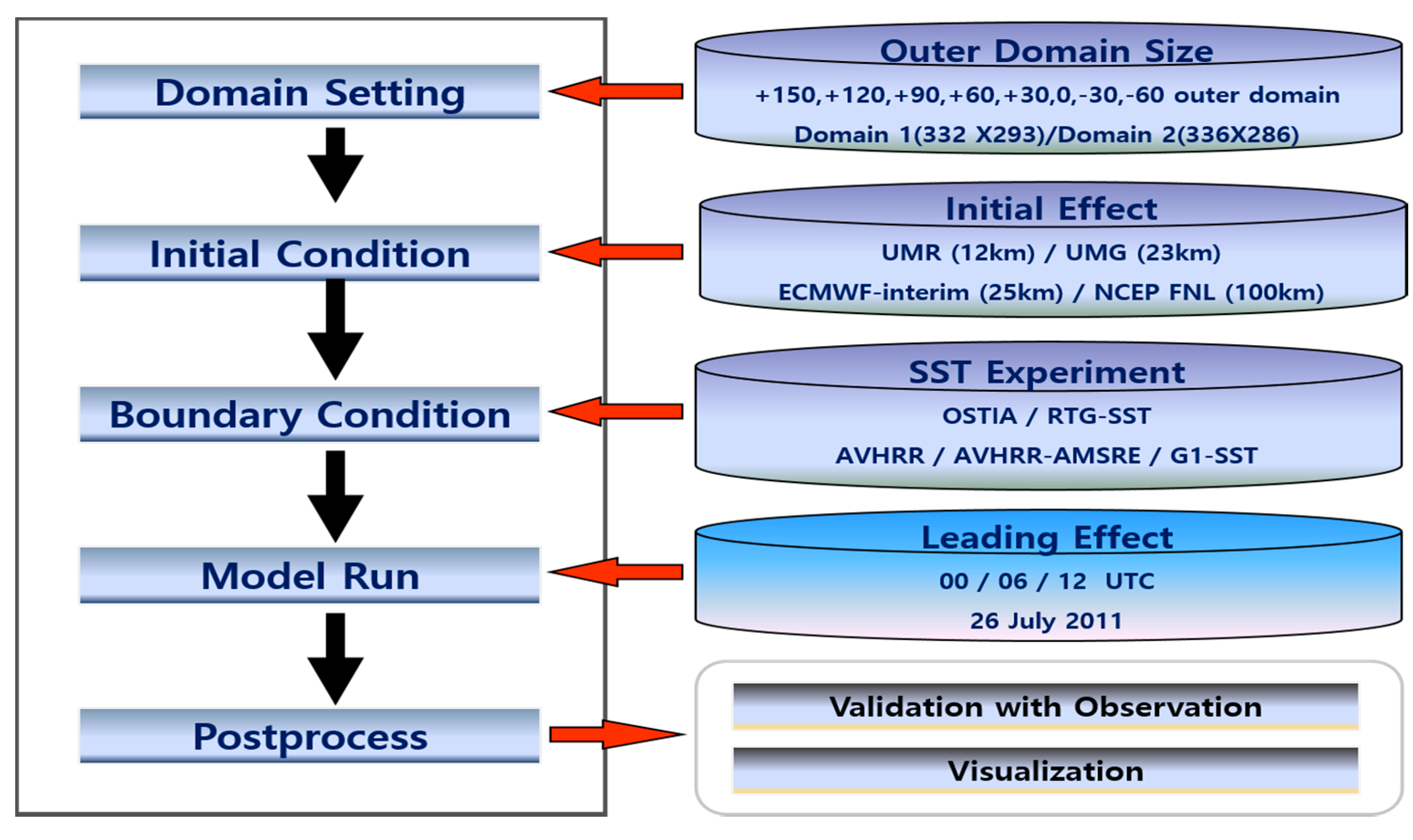
In the previously configured WRF system, there are model configuration and data incorporation processes that influence the model performance, such as outer domain size, sea surface temperature data, initial conditions, and lead time effect (Figure 6). In the present study, a series of sensitivity tests were performed by changing the model configuration and input data source.
Table 2 summarizes all the experiments performed, and each sensitivity experiment consists of various simulations that have model inputs or configurations different from those of the default model. Note that lead times of 18, 12, and 6 h mean that the model starts at 18, 12, and 6 h before 18 UTC 26 July 2011, which are 00 UTC, 6 UTC, and 12 UTC on 26 July 2011, respectively. See a more detailed explanation of each experiment in the following subsection.
3.1. Impact of Domain Size
There is no “rule of thumb” for configuring a domain for WRF, and nesting options with ratios (inner to outer domain) of 3, 4, and 5 are available. This study employed a ratio of 5 so that the inner and outer domains had resolutions of 1 and 5 km, respectively. As mentioned previously, such a resolution was chosen because the KLAPS is operated by the KMA for a very short-range high-resolution numerical prediction with 15-km resolution for the outer domain and 5-km data-assimilated nested inner domain. In addition, a smoother transition from the outer domain to the inner domain is important to prevent numerical instabilities around the borders as well as propagation of numerical artifacts into the center of the domain. Therefore, the model configuration for the inner domain was retained for all simulations, opting for an ample buffer zone of five grid points and an exponential transition at the border.
Previous studies showed that different domains might be required for different sub-regions within the model domain to produce mean precipitation close to observations over the study region [9,26]. To evaluate the effects of such transitions on precipitation forecasting for the inner domain, the size of the outer domain was increased or decreased such that a number of grids from −60 to +150 by increments of +30 was added to the basic configuration of the outer domain for all directions (dashed rectangular boxes from the interior to the exterior in Figure 1a). A domain size of 0 indicates the default model configuration. Figure 7 shows the simulation results of the forecasting model over the inner domain for various outer domain sizes. For better comparison, the AWS rainfall analysis field shown in Figure 4a is also shown in Figure 7, in which the rainband is located over northeast Seoul.
The model results show the effect of the outer domain size on the performance of the inner domain. Figure 7b–f clearly show that the precipitation range gets progressively wider and the location of the rainfall band moves southward closer to Seoul as the outer domain size is decreased. Subsequent decreases in size result in insignificant changes in the precipitation range and location of the rainband (Figure 7f–i). When compared with the observation, a smaller outer domain size produces a better performing forecasting model. That is, given the inner domain size for the forecasting model, the model performance is better with smaller outer domain sizes relative to larger outer domain sizes. This occurs partly because under larger outer domains, the northeastward synoptic wind drives the rainfall band over the northeast side of Seoul, and the rainfall core and its rainband are located too far north of the target area. Therefore, the initial/boundary conditions for the inner domain are relatively well represented by those of a smaller outer domain. Additionally, the 2-m temperature shows similar behavior to the precipitation, such that the temperature drop is shown more clearly in the smaller outer domain size than in the default (figure not shown). The second onset of rainfall is also better represented by the smaller domains than the larger domains.
3.2. Sea Surface Temperature
Both the moisture flux convergence and moisture availability over adjacent oceans are important factors in heavy rainfall events [27,28]. The Yellow Sea is located on the west coast of the Korean Peninsula, a tide-dominated area with a complex coastal shape and many islands (Figure 1a). This marginal sea is a well-known shallow sea with an average depth of about 40 m. Rainfall events obtain additional moisture when they travel over the sea and develop heavy rainfall features. In this section, the impact of the Sea Surface Temperature (SST) of the Yellow Sea on the heavy rainfall over inland Korea is evaluated.
Input data for SST from different sources were incorporated to evaluate the performance of the forecasting model. The SST data were obtained from the OSTIA, with approximately 5-km resolution (default option); the Real-Time, Global, Sea Surface Temperature (RTG_SST) analysis, with about 900-m resolution; the Advanced Very-High-Resolution Radiometer (AVHRR), with 1-km resolution; the Advanced Microwave Scanning Radiometer-EOS (AMSR-E) blended with AVHRR (AVHRR+AMSRE); the Global 1 km Sea Surface Temperature (G1-SST), which includes AVHRR, AMSR-E, in situ data from drifting and moored buoys, and other radiometer and satellite images.
Figure 8 shows the daily accumulated rainfall in the inner domain from 00 UTC 26 July 2011 to 00 UTC 27 July 2011. The spatial patterns of the heavy rainfall cores for all simulations are similar in that the cores are shifted southeastward, but the weak rainfall cores from the default of OSTIA are more widely spread than those from the other SST data. Although spatially different patterns exist among the SST data, the simulation results do not show much difference. This is partly due to the small magnitude in the differences between the SST data. The maximum differences for the precipitation and 2-m temperature time series among simulations are less than 2 mm/h and 1.4 °C, respectively. In this experiment, there is no significant effect on the second onset in any simulation. That is, the detailed analysis of SST and its diurnal cycle may not be needed in the short-range high resolution forecasting model because these vary too slowly to affect the model in this study.
However, it is worth noting that sometimes the initial input of SST plays a key role in other severe weather, especially in the case of important precipitation events, which are dependent on evaporation. Previously, Manda et al. [27] showed the impacts of the Yellow Sea on torrential rainfall organized under the Asian Summer Monsoon and found that heavy rainfall will increase significantly under the projected warming of the marginal sea and overlying atmosphere.
3.3. Initial Conditions
Higher resolution forecast models generally have greater sensitivity and dependency on initial conditions than coarser resolution models [28]. In this experiment, various initial conditions for the 5-km outer domain were simulated to evaluate their effects on the precipitation forecasting performance of the forecasting model. As indicated previously, the initial and boundary conditions were obtained as a default simulation by spatial interpolation of the 12-km UM regional model forecast (UMR) field of 70 vertical layers, which is assimilated from KMA data, such as radar, AWS, satellite, and profile data. For other sensitivity simulations, various initial conditions were used for meteorological variables that were initialized from the UM Global Prediction Model (UMG) at 23-km resolution with 70 vertical layers, the ECMWF Interim Reanalysis (ERA-interim) at 25-km resolution (interpolated from 0.75 degrees resolution) with 60 vertical layers, and the NCEP-FNL at 100-km resolution with 27 vertical layers. Time-varying lateral boundary conditions were provided every 1 h for UMR, every 3 h for UMG, and every 6 h for ERA-interim and NCEP-FNL.
Figure 9 shows the daily accumulated rainfall model results for all simulations. The maximum rainfall for UMR and NCEP-FNL are similar to the observation in Figure 7a, but the rainband locations are skewed southwest in UMR, and northwest in NCEP-FNL. For UMG and ECMWF-interim, both results provide relatively poor representation of the rainband location and rainfall amount compared to those for UMR and NCEP-FNL. The initial condition for NCEP-FNL uses the coarser resolution data than the other initial conditions, but the performance of the forecasting model is relatively good in terms of the precipitation amount and rainband location. This suggests that for better convective initiation, better data assimilations directly applied at the regional scale, with the possible inclusion of local observations, are needed. Experimental results suggest that the performance of the high resolution forecasting model is sensitive to the initial conditions regardless of the resolution of the initial conditions. In order to improve the accuracy of precipitation for the forecasting model, the results also imply that ensemble forecasting with various initial conditions could be a good strategy.
3.4. Lead Time Effect
Lead time generally refers to how long the forecasting is simulated by the NWP model, but the lead time here is the latency between the initiation and the target time of 18 UTC 26 July 2011. Previous studies of the lead time effect over Korea, such as the study by Jang and Hong [24], suggested that both the effects of horizontal resolution and lead time should be considered for forecasting heavy rainfall, but with greater weighting on horizontal resolution because heavy rainfall over Korea is primarily a mesoscale phenomenon. For a 1-km high-resolution model, the systematic behavior of such lead time features has not yet been articulated. However, it seems clear that for forecasting models of resolution <1 km, the lead time becomes very important because the accuracy of precipitation forecasts embedded in the initial conditions decreases. In addition, it is generally accepted that numerical models behave differently with varying model configurations, target regions, or target forecasting times. In particular, the lead time experiments can provide some insights to end-users on the best numerical model performance given a specific forecasting time.
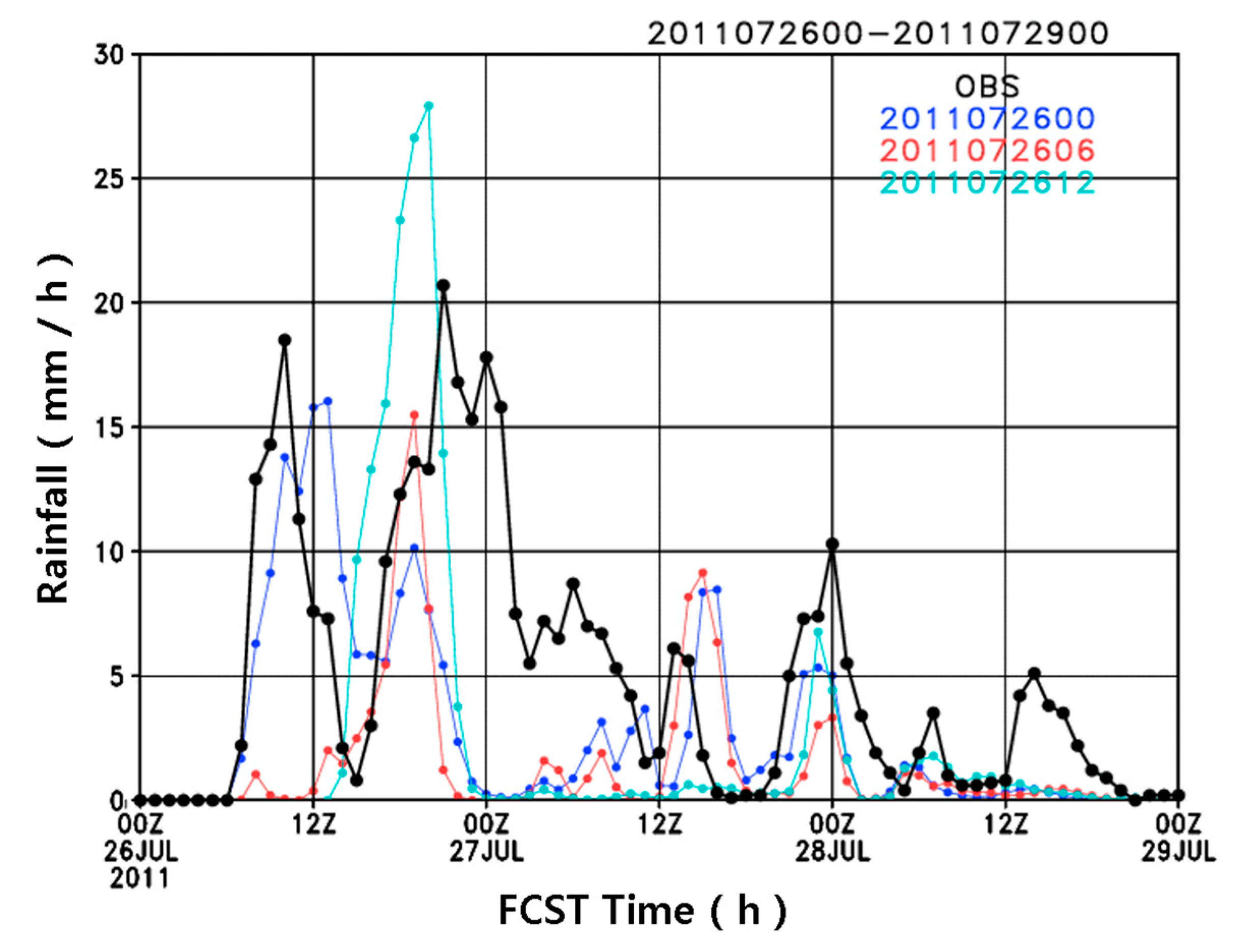
Figure 10 shows the hourly accumulated precipitation results at 18 UTC 26 July 2011 for the lead time effect experiment, which was initiated at 00 UTC (default option), 06 UTC, and 12 UTC 26 July 2011. In all simulations, heavy rainfall is predictable although biases still exist for the rainband location and magnitude of precipitation. Additionally, two initial conditions that are 6 h apart result in quite different rainband locations. With a lead time of +12 h, the rainband is located north of Seoul and subsequently dies out gradually. As the lead time decreased and became close to the target time of 18 UTC 26 July 2011, such as for the forecast model initiated at 12 UTC 26 July 2016, the result became more similar to the observations in Figure 6a; the rainband was located over Seoul and the precipitation magnitude improved.
Figure 11 shows the time series of the spatially averaged hourly rainfall indicated by the boxes in Figure 10 (37.3° N–37.8° N, 126.6° E–127.4° E). For the second onset of the rainfall, as the lead time is close to the target time (1800 UTC 26 July 2011), the maximum accumulated precipitation from the forecasting model gets larger, but the duration of precipitation is similar for all simulations. The lead time experiment for the high-resolution forecasting model in this study indicates that a lead time <6 h might be appropriate for very-short range numerical forecasting over the region of Seoul, Korea. It is worth noting that for the shorter than 3-h lead time precipitation forecast, the radar data extrapolation is usually more accurate than the numerical weather prediction.
3.5. Discussion
The sensitivity experimental results in this study show that the high-resolution forecasting model at 1-km resolution performed better than the coarse-resolution model at 5-km resolution for all simulations. Therefore, the dynamical downscaling method seems to be effective via the WRF nesting process. In addition, the sensitivity analysis suggests that for a given forecasting model, an appropriate outer domain size and lead time for a high-resolution model should be taken into consideration to optimize the WRF configuration for regional torrential rainfall events around Seoul and its suburban area. That is, given the default model results as a reference, the experiments with a relatively small outer domain and short lead time produced a more accurate distribution and intensity of precipitation than the other experiments. Larger domain sizes and longer lead times led to larger internal variabilities in the forecasting model, resulting in displacements of the rainfall band. More informative initial conditions are more useful than high resolution initial conditions for the performance of the forecasting model. Finally, SST experiments show negligible influence and do not capture short-term model variability.
Table 3 quantitatively confirms the results of the sensitivity experiments using indices of precipitation prediction evaluation, such as Probability of Detection (POD), False Alarm Ratio (FAR), and Equitable Threat Score (ETS). The POD, known as the hit rate, measures the fraction of observed events that were correctly forecast, FAR provides the fraction of forecast events that were observed as non-events, and ETS accounts for the hits that would occur purely due to random chance [29]. Given the inner domain size for the 1-km resolution forecasting model, an appropriate outer domain size is an important factor in precipitation forecasting in Korea; these factors influence the correct location of the rainfall core and rainband in the high resolution model. In large outer domains, the rainfall bands are located too far north of the target area compared to those observed in the regional models [24]. For the SST experiment, there are no significant differences in the indices between simulations, and the SST data do not impact the shorter lead time forecasts [30]. SST could have more influence on forecasting precipitation by coupling the atmosphere model and ocean models. The experiments for both initial conditions and lead time showed large influences on the performance of precipitation forecasting of the very short-time high-resolution models. To make substantial improvements in short-range precipitation forecasting, we need to improve the initial conditions through data assimilation, and determine the appropriate outer domain sizes and effective lead times.
Table 4 shows a statistical summary of the sensitivity studies. To compare simulation results with observations, the 54 AWSs were used to calculate the correlation coefficient (CC), deviation (BIAS), and root mean square error (RMSE). The statistics shown in Table 4 indicate the 2-m temperature (T2), 10-m wind speed (WS10), and relative humidity (Rh) variables. For each variable, the shading indicates the CC closest to one, lowest RMSE, and BIAS values closest to zero for each experiment. The statistical results indicate that the model results from the smaller outer domains and shorter lead times perform better statistically than those from larger domains and longer lead times. Goswami et al. [13] investigated this issue using >10 km resolutions and the Fifth-generation Penn State/NCAR Mesoscale Model (MM5) simulations for three high-impact weather (heavy rainfall) events over the Tropics to establish the best model performance. Their results showed that domain size is as important as grid spacing and initial conditions in the simulating high-impact weather events. The results showed that, along with initial conditions and grid size, the domain size also significantly affects simulated quantities, such as total and maximum rain.
Overall, the sensitivity analyses of model performances have traditionally focused on model physics, initial conditions, and SST. Analyses associated with outer domain size and lead time are rarely considered. The results of the precipitation forecast illustrated by the statistical skill scores in Table 3 and Table 4 show that the impacts of the model outer domain and lead time are as large as those of the initial conditions. That is, the impacts of various model configurations, such as the outer domain size, initial conditions, and lead time, are greater than those of SST on the performance of precipitation forecasting from high-resolution models in short-time forecasts. It is worth noting that the resulting sensitivity exhibits case-by-case variability. For example, Wang et al. [9] performed sensitivity studies for three different cases. They concluded that their precipitation forecasting was only slightly affected by initial conditions and model physics in the longer-time forecast, and, while they had similar properties, there was still case-by-case variability.
4. Summary and Remarks
Sensitivity analyses have traditionally focused on model physics and initial conditions, but the model uncertainty associated with domain size and model resolution has been rarely considered [9]. This work performed a sensitivity study on high-resolution WRF precipitation forecasts for a heavy rainfall event over Seoul, the capital city of Korea, for 26 and 27 July 2011. WRF simulation results were analyzed with various configurations, including outer domain size, sea surface temperature, initial conditions, and lead time. The study indicates that the impacts of domain size and lead time on the precipitation forecasts were no less significant than those of initial field conditions and SST data.
As mentioned previously, the combination of optimal choices presented here may not be the optimal configuration for a given forecasting model, and fine-resolution input data generally, but not always, show good performance. Min et al. [31] studied the effect of outer domain size on forecasting models and reported that the biggest outer domain initialized with the NCEP-FNL initial conditions produced a better performing forecasting model. The combination of initial conditions from NCEP-FNL and RTG-SST data yielded a similar result to those from UMR and OSTIA SST (figure not shown). That is, NCEP-FNL data are very coarse but still yield very good forecasting results in some cases. This is partly because the initial condition is a well data-assimilated analysis field and combines with an appropriate configuration. Jee and Kim [16] also showed that topographical terrain data with a resolution higher than the model resolution results in significant improvement in the representation of topographical heights and land use, but did not produce a statistically significant improvement in model performance.
This study adopted the same configuration for the physical parameterizations as the Korean Local Analysis and Prediction System operational model that is run by KMA. For precipitation forecasting, the parameterization of microphysics and convective schemes is generally the most important consideration because these schemes have a direct effect on the generation, distribution, and intensity of precipitation. When the horizontal resolution is in the <10 km range, the precipitation behavior of a numerical model with and without those parameterized schemes should be explored systematically. Increasing the skill of forecasting precipitation with various parameterized schemes remains for further study [32].
Furthermore, although the high-resolution forecasting model is optimized, the deterministic model might still have several problems to resolve, such as short range severe weather events, i.e., heavy precipitation. In such an environment, the predictability of the forecasting model could be improved by considering the probabilistic forecast. Ensemble prediction systems are more applicable to high-impact weather forecasting by adding some probabilistic values to the deterministic forecasting model. Additionally, although we would perform additional intensive sensitivity studies regarding the domain size, lead time, and so on for a vast majority of severe weather events, the optimized configuration for the high-resolution forecasting model might not be achieved. In such cases, sophisticated data assimilation techniques could be the alternative for improving the performance of the high-resolution forecasting model. We leave these experiments of high-resolution model forecasts for future studies.
Acknowledgments
The authors thank the reviewers for their very valuable comments and the managing editor and assistant editor for constructive suggestions, which greatly improved the quality of the paper. We especially thank KMA's supercomputer management division for providing us with the supercomputer resource and consulting on technical support. This work was funded by the Weather Information Service Engine Program of the Korea Meteorological Administration under Grant KMIPA-2012-0001-1.
Author Contributions
J.-B. Jee and S. Kim conceived and designed the experiments, analyzed the data and the model results, and wrote the article; J.-B. Jee performed the experiments and the statistical calculation.
Conflicts of Interest
The authors declare no conflict of interest.
References
- Heavy Rainfall Events Top 10 (in Korean); KMA Registered PUB, No. 11-136000-000833-01; Korea Meteorological Administration: Seoul, Korea, 2011.
- Skamarock, W.C.; Klemp, J.B.; Dudhia, J.; Gill, D.O.; Barker, D.M.; Duda, M.G.; Huang, X.; Wang, W.; Powers, J.G. A Description of the Advanced Research WRF Version 3; NCAR Tech. Note (NCAR/TN-475+STR); National Center for Atmospheric Research: Boulder, CO, USA, 2008; p. 125. [Google Scholar]
- Hong, S.-Y.; Park, H.; Cheong, H.-B.; Kim, J.-E.; Koo, M.-S.; Jang, J.; Ham, S.; Hwang, S.-O.; Park, B.-K.; Chang, E.-C.; et al. The global/regional integrated model system (GRIMs). Asia Pac. J. Atmos. Sci. 2013, 49, 219–243. [Google Scholar] [CrossRef]
- Zhang, C.; Lin, H.; Chen, M.; Yang, L. Scale matching of multiscale digital elevation model (DEM) data the Weather Research and Forecasting (WRF) model: A case study of meteorological simulation in Hong Kong. Arab. J. Geosci. 2014, 7, 2215–2223. [Google Scholar] [CrossRef]
- Paviva, L.M.; Bodstein, G.C.R.; Pimentel, L.C.G. Influence of high-resolution surface databases on the modeling of local atmospheric circulation systems. Geosci. Model Dev. 2014, 7, 1641–1659. [Google Scholar] [CrossRef]
- Nunalee, C.G.; Horváth, Á.; Basu, S. High-Resolution numerical modeling of mesoscale island wakes and sensitivity to static topographic relief data. Geosci. Model Dev. 2015, 8, 2645–2653. [Google Scholar] [CrossRef]
- Zheng, Y.; Alapaty, K.; Jerold, A.; Herwehe, J.A.; Del Genio, A.D.; Niyogi, D. Improving High-Resolution Weather Forecasts Using the Weather Research and Forecasting (WRF) Model with an Updated Kain–Fritsch Scheme. Mon. Weather Rev. 2016, 144, 833–860. [Google Scholar] [CrossRef]
- Choi, Y.; Kang, S.-L.; Hong, J.; Grimmond, S.; Davis, K.J. A next-generation Weather Information Service Engine (WISE) customized for urban and surrounding rural areas. Bull. Am. Meteorol. Soc. 2013, 94, ES114–ES117. [Google Scholar] [CrossRef]
- Wang, X.; Steinle, P.; Seed, A.; Xiao, Y. The Sensitivity of Heavy Precipitation to Horizontal Resolution, Domain Size, and Rain Rate Assimilation: Case Studies with a Convection-Permitting Model. Adv. Meteorol. 2016, 2016, 7943845. [Google Scholar] [CrossRef]
- Dravitzki, S.; McGregor, J. Predictability of heavy precipitation in the Waikato River basin of New Zealand. Mon. Weather Rev. 2011, 139, 2184–2197. [Google Scholar] [CrossRef]
- Goswami, P.; Shivappa, H.; Goud, S. Comparative analysis of the role of domain size, horizontal resolution and initial conditions in the simulation of tropical heavy rainfall events. Meteorol. Appl. 2012, 19, 170–178. [Google Scholar] [CrossRef]
- Goswami, P.; Mohapatra, G.N. A comparative evaluation of impact of domain size and parameterization scheme on simulation of tropical cyclones in the Bay of Bengal. J. Geophys. Res. Atmos. 2014, 119, 10–22. [Google Scholar] [CrossRef]
- Li, Y.; Lu, G.; Wu, Z.; He, H.; Shi, J.; Ma, Y.; Weng, S. Evaluation of Optimized WRF Precipitation Forecast over a Complex Topography Region during Flood Season. Atmosphere 2016, 7, 145. [Google Scholar] [CrossRef]
- Ha, J.-C.; Lee, Y.-H.; Lee, H.C.; Nam, J.-E.; Lee, J.S. The Operational Manual of Korea Local Analysis and Prediction System; NIMR-TN-2011-006; National Institute of Meteorological Research: JeJu, Korea, 2011; 55p.
- Kim, E.-H.; Ahn, K.-D.; Lee, H.-C.; Ha, H.-C.; Lim, E. A study on the effect of ground-based GPS data assimilation into very-short-range prediction model. Atmosphere 2015, 25, 623–637, (In Korean with English Abstract). [Google Scholar] [CrossRef]
- Jee, J.-B.; Kim, S. Sensitivity Study on High-Resolution Numerical Modeling of Static Topographic Data. Atmosphere 2016, 7, 86. [Google Scholar] [CrossRef]
- Hong, S.-Y.; Noh, Y.; Dudhia, J. A new vertical diffusion package with an explicit treatment of entrainment processes. Mon. Weather Rev. 2006, 134, 2318–2341. [Google Scholar] [CrossRef]
- Lim, K.-S.S.; Hong, S.-Y. Development of an effective double-moment cloud microphysics scheme with prognostic cloud condensation nuclei (CCN) for weather and climate models. Mon. Weather Rev. 2010, 138, 1587–1612. [Google Scholar] [CrossRef]
- Tewari, M.; Chen, F.; Wang, W.; Dudhia, J.; LeMone, M.A.; Mitchell, K.; Ek, M.; Gayno, G.; Wegiel, J.; Cuenca, R.H. Implementation and verification of the unified NOAH land surface model in the WRF model. In Proceedings of the 20th Conference on Weather Analysis and Forecasting/16th Conference on Numerical Weather Prediction, Boulder, CO, USA, 10–12 January 2004; pp. 11–15. [Google Scholar]
- Chou, M.D.; Suarez, M.J. A Solar Radiation Parameterization for Atmospheric Studies; Technical Report Series on Global Modeling and Data Assimilation; NASA Goddard Space Flight Center: Greenbelt, MD, USA, 1999.
- Lee, D.-K.; Kim, H.-R.; Hong, S.-Y. Heavy rainfall over Korea during 1980–1990. Korean J. Atmos. Sci. 1998, 1, 32–50. [Google Scholar]
- Rha, D.-K.; Kwak, C.-H.; Suh, M.-S.; Hong, Y. Analysis of the characteristics of precipitation over South Korea in terms of the associated synoptic patterns: A 30 years climatology (1973–2002). J. Korean Earth Sci. Soc. 2005, 26, 732–743, (In Korean with English Abstract). [Google Scholar]
- Sun, J.; Lee, T.-Y. A numerical study of an intense quasistationary convection band over the Korean peninsula. J. Meteorol. Soc. Jpn. 2002, 80, 1221–1245. [Google Scholar] [CrossRef]
- Jang, J.; Hong, S.-Y. Quantitative forecast experiment of a heavy rainfall event over Korea in a global model: Horizontal resolution versus lead time issues. Meteorol. Amos. Phys. 2014, 124, 113–127. [Google Scholar] [CrossRef]
- Ebert, E.E.; Damrath, U.; Wergen, W.; Baldwin, M.E. The WGNE assessment of short-term quantitative precipitation forecasts. Bull. Am. Meteorol. Soc. 2003, 84, 481–492. [Google Scholar] [CrossRef]
- Bhaskaran, B.; Ramachandran, A.; Jones, R.; Moufouma-Okia, W. Regional climate model applications on sub-regional scales over the Indian monsoon region: The role of domain size on downscaling uncertainty. J. Geophys. Res. Atmos. 2012, 117. [Google Scholar] [CrossRef]
- Manda, A.; Nakamura, H.; Asano, N.; Iizuka, S.; Miyama, T.; Moteki, O.; Yoshioka, M.K.; Nishii, K.; Miyasaka, T. Impacts of a warming marginal sea on torrential rainfall organized under the Asian summer monsoon. Sci. Rep. 2014, 4, 5741. [Google Scholar] [CrossRef] [PubMed]
- Mittermaier, M.P. Improving short-range high-resolution model precipitation forecast skill using time-lagged ensembles. Q. J. R. Meteorol. Soc. 2007, 133, 1487–1500. [Google Scholar] [CrossRef]
- Ebert, E.E. Fuzzy verification of high-resolution gridded forecasts: A review and proposed framework. Meteorol. Appl. 2008, 15, 51–64. [Google Scholar] [CrossRef]
- Etherton, B.; Santos, P. Sensitivity of WRF Forecasts for South Florida to Initial conditions. Weather Forecast. 2008, 23, 725–740. [Google Scholar] [CrossRef]
- Min, J.-S.; Rho, J.-W.; Jee, J.-B.; Kim, S. A study on sensitivity of heavy precipitation to domain size with a regional numerical weather prediction model. Atmosphere 2016, 26, 85–95. [Google Scholar] [CrossRef]
- Sikder, S.; Hossain, F. Assessment of the weather research and forecasting model generalized parameterization schemes for advancement of precipitation forecasting in monsoon-driven river basins. J. Adv. Model. Earth Syst. 2016, 8, 1210–1228. [Google Scholar] [CrossRef]
Figure 1.
Default model domains for (a) the 5 km outer domain indicated by the black solid rectangular box identified as s1; (b) the 1 km inner domain (red rectangular box identified as d02 in Figure 1a); and (c) Automated Weather Station (AWS) locations with red dots and the digital elevation model (DEM) with shading (black box in Figure 1b). White dot and black dashed rectangular boxes in (a) respectively indicate the domain reference grid (36° N latitude, 126° E longitude) and numerical outer domains for the sensitivity experiments. The black dot in (b) and white dot in (c) indicate the AWS location of the Seocho meteorological station (37.49° N latitude, 127.02° E longitude). Red dots in (c) indicate AWS sites in urban and rural areas. The solid closed curve in (b,c) represent the administrative district for Seoul.
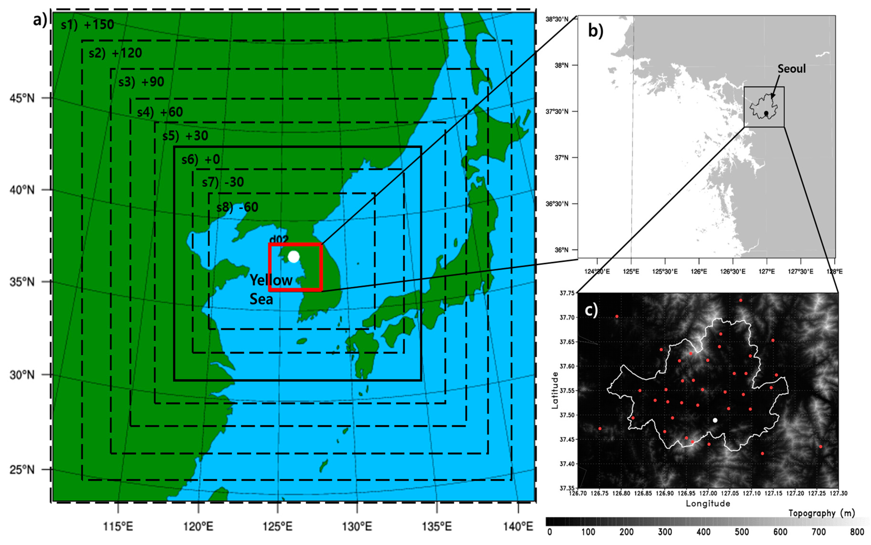
Figure 2.
Weather chart provided by KMA for (a) 00 UTC 26 July 2011; (b) 12 UTC 26 July 2011; and (c) 00 UTC 27 July 2011.
Figure 2.
Weather chart provided by KMA for (a) 00 UTC 26 July 2011; (b) 12 UTC 26 July 2011; and (c) 00 UTC 27 July 2011.
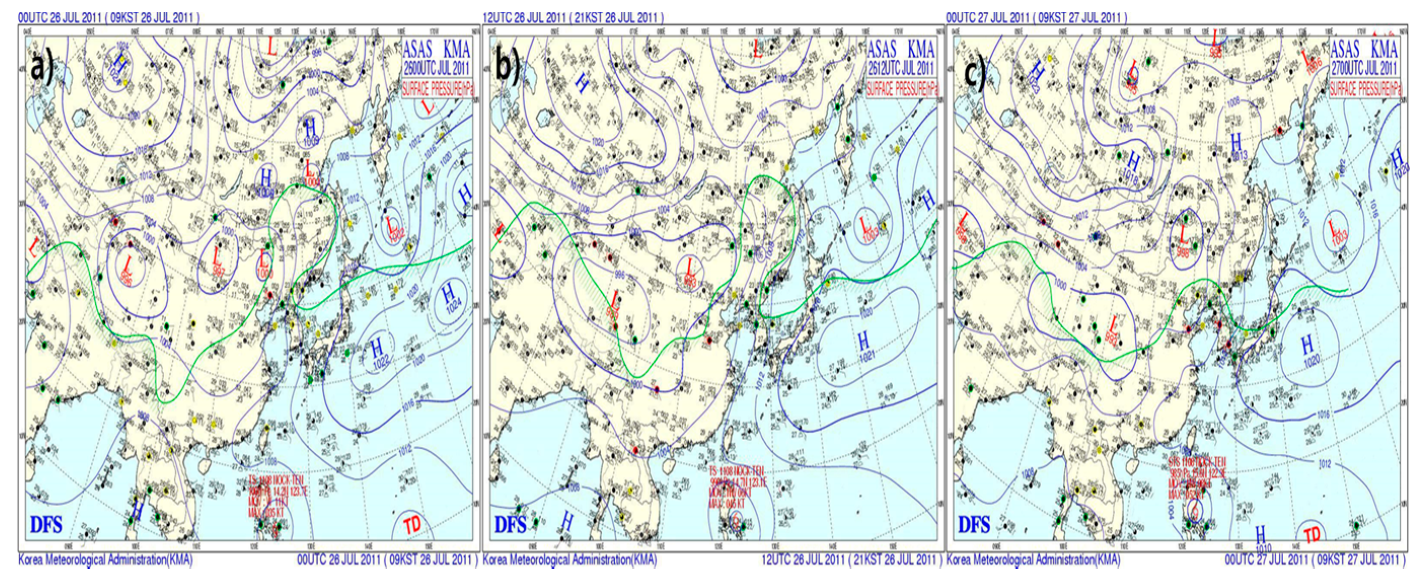
Figure 3.
KMA-observed hourly accumulated rainfall at 18 UTC 26 July 2011 for (a) radar; (b) AWSs; and (c) meteogram of the Seocho Meteorological Station (white dot in Figure 1c). The color bar represents the rain rate (mm/h) in (a,b). Meteorological values in the meteogram include one-hour accumulated rainfall (blue shading), 15 min accumulated rainfall (magenta shading), rain detection (sky-blue shading), temperature (red line), wind speed (green line), and wind direction (orange dots) from 00 UTC 26 July 2011 to 15 UTC 27 July 2011.

Figure 4.
One-hour accumulated rainfall at 18 UTC 26 July 2011 for (a) AWS analysis field; (b) 5 km outer domain part; and (c) 1 km inner domain. The color bar represents the rain rate (mm/h). The box in each panel indicates the region bounded by 37.3° N–37.8° N and 126.6° E–127.4° E.
Figure 4.
One-hour accumulated rainfall at 18 UTC 26 July 2011 for (a) AWS analysis field; (b) 5 km outer domain part; and (c) 1 km inner domain. The color bar represents the rain rate (mm/h). The box in each panel indicates the region bounded by 37.3° N–37.8° N and 126.6° E–127.4° E.
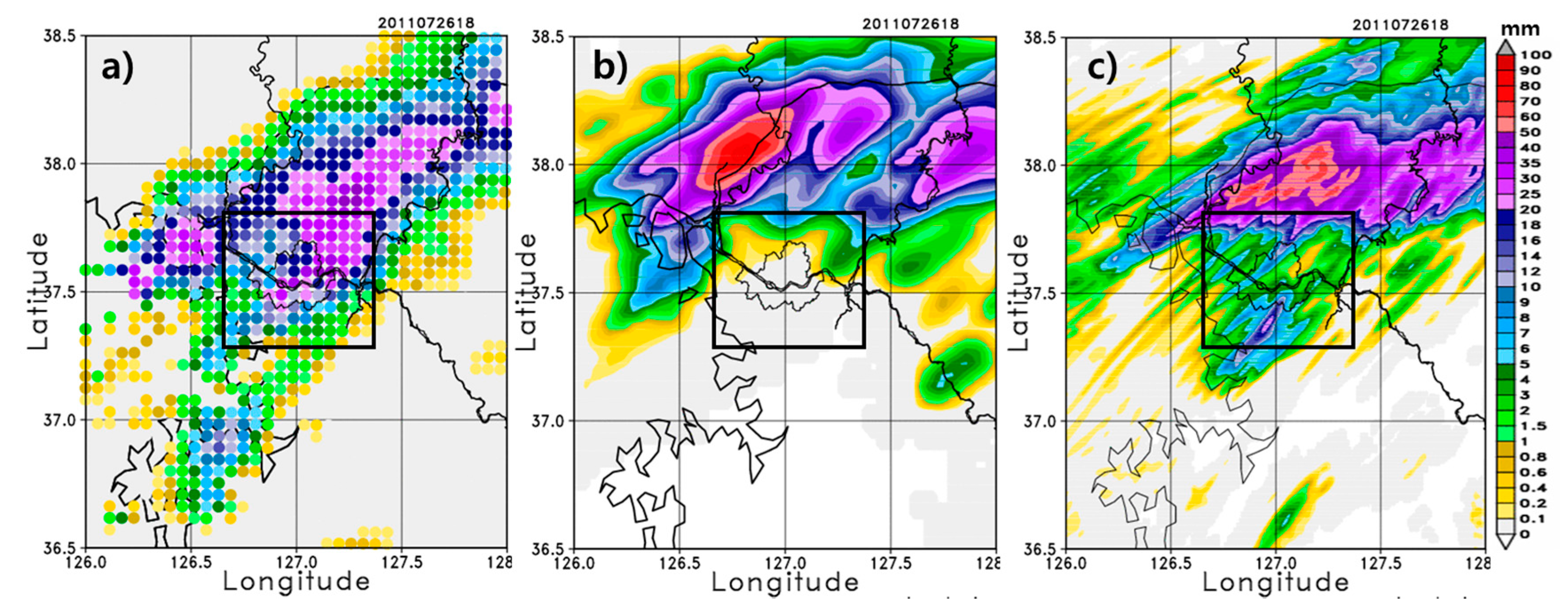
Figure 5.
Domain-averaged hourly accumulated rainfall averaged between latitudes 37.49° N and 37.8° N, and between longitudes 126.6° E and 127.4° E for the AWS analysis field (black line), outer domain (red line), and inner domain (blue line). The horizontal axis is the forecasting time starting at 00 UTC 26 July 2011. The two ellipses indicate the first and second onsets of rainfall at the beginning of the rainfall period.

Figure 6.
Flowchart of the WRF sensitivity simulations. The left column is the order of the model run, and the right column shows the necessary data source incorporated into the WRF depending on the experiments shown in Table 2.
Figure 6.
Flowchart of the WRF sensitivity simulations. The left column is the order of the model run, and the right column shows the necessary data source incorporated into the WRF depending on the experiments shown in Table 2.

Figure 7.
Effect of outer domain size on the performance of the inner domain for hourly accumulated precipitation at 18 UTC 26 July 2011. (a) AWS rainfall analysis provided by KMA. Sensitivity results of the inner domain for (b) +150; (c) +120; (d) +90; (e) +60; (f) +30; (g) 0; (h) −30; and (i) −60, respectively, for the outer domain sizes of (s2), (s3), (s4), (s5), (s6), (s1), (s7), and (s8) in Figure 1a. The color bar represents the rain rate (mm/h).
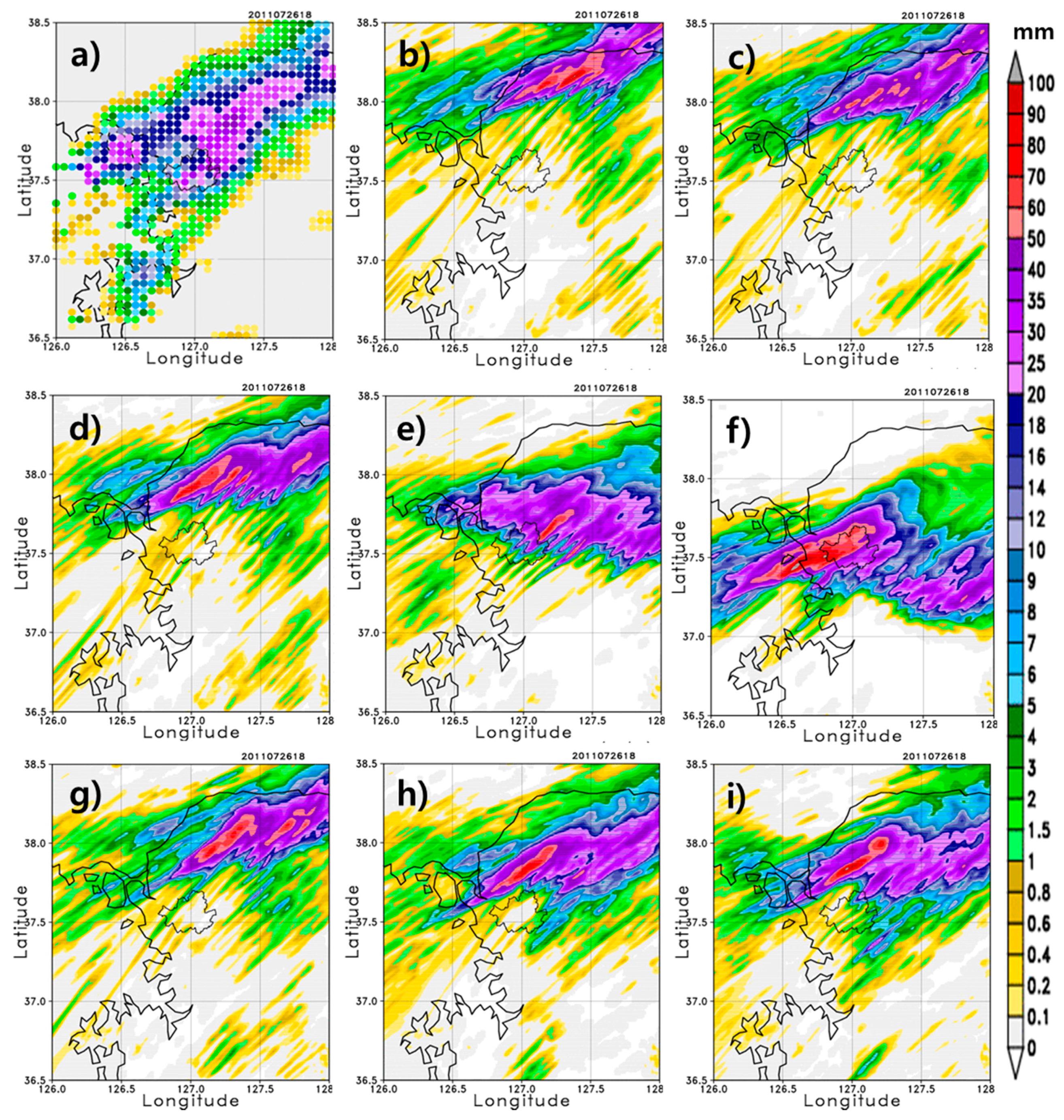
Figure 8.
SST effects of daily accumulated rainfall between 00 UTC 26 July 2011 and 00 UTC 27 July 2011 for (a) AWS rainfall analysis by KMA, and model SST experiments for (b) OSTIA, (c) RTG-SST, (d) AVHRR, (e) AVHRR-AMSRE, and (f) G1-SST. The color bar represents the rain rate (mm/day).
Figure 8.
SST effects of daily accumulated rainfall between 00 UTC 26 July 2011 and 00 UTC 27 July 2011 for (a) AWS rainfall analysis by KMA, and model SST experiments for (b) OSTIA, (c) RTG-SST, (d) AVHRR, (e) AVHRR-AMSRE, and (f) G1-SST. The color bar represents the rain rate (mm/day).
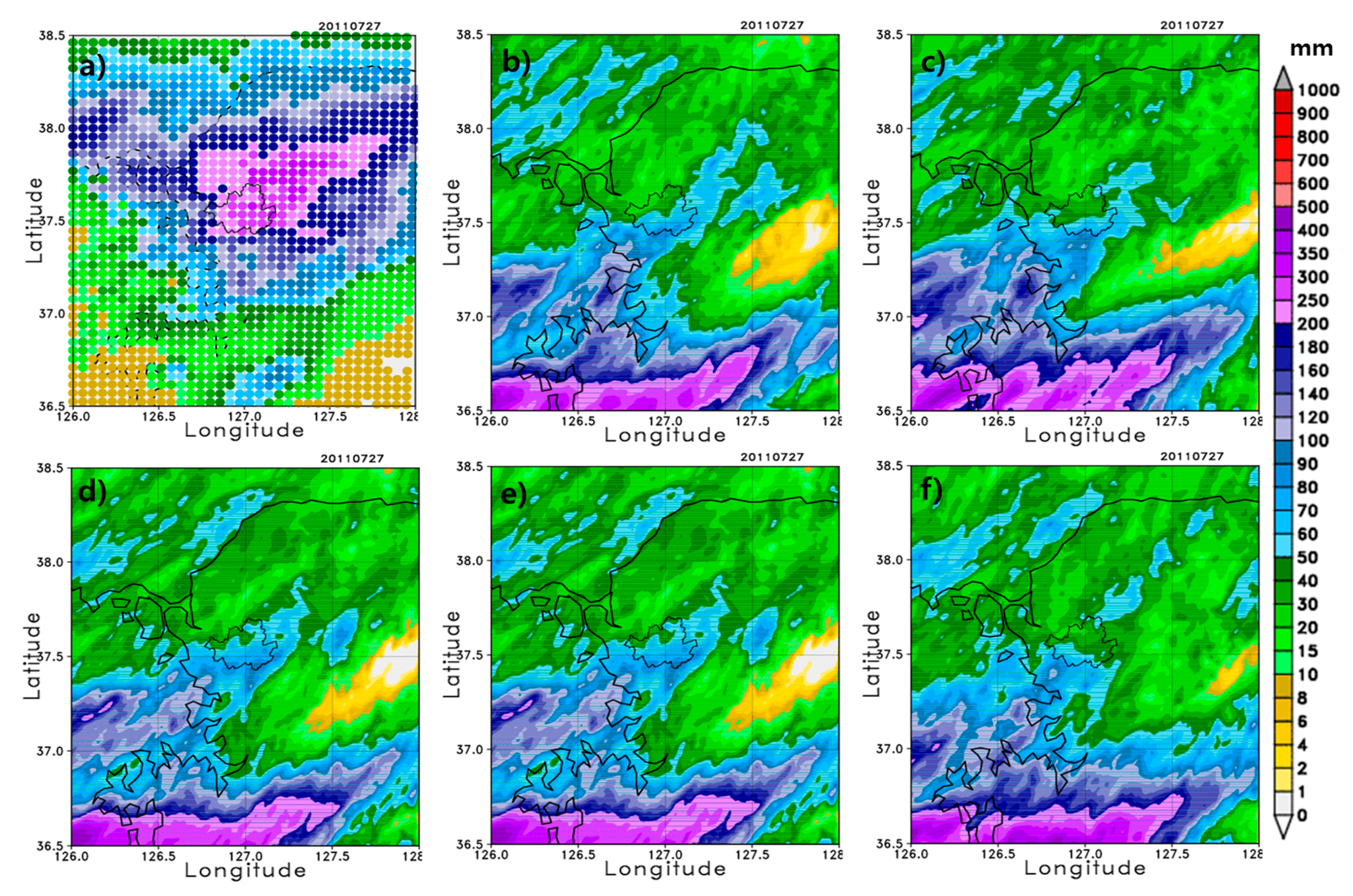
Figure 9.
Effect of the initial conditions on the daily accumulated rainfall between 00 UTC 26 July 2011 and 00 UTC 27 July 2011. (a) UMR (12 km); (b) UMG (23 km); (c) ECMWF-interim; (d) NCEP-FNL. See Figure 7a for a comparison with the AWS rainfall analysis. The color bar represents the rain rate (mm/day).
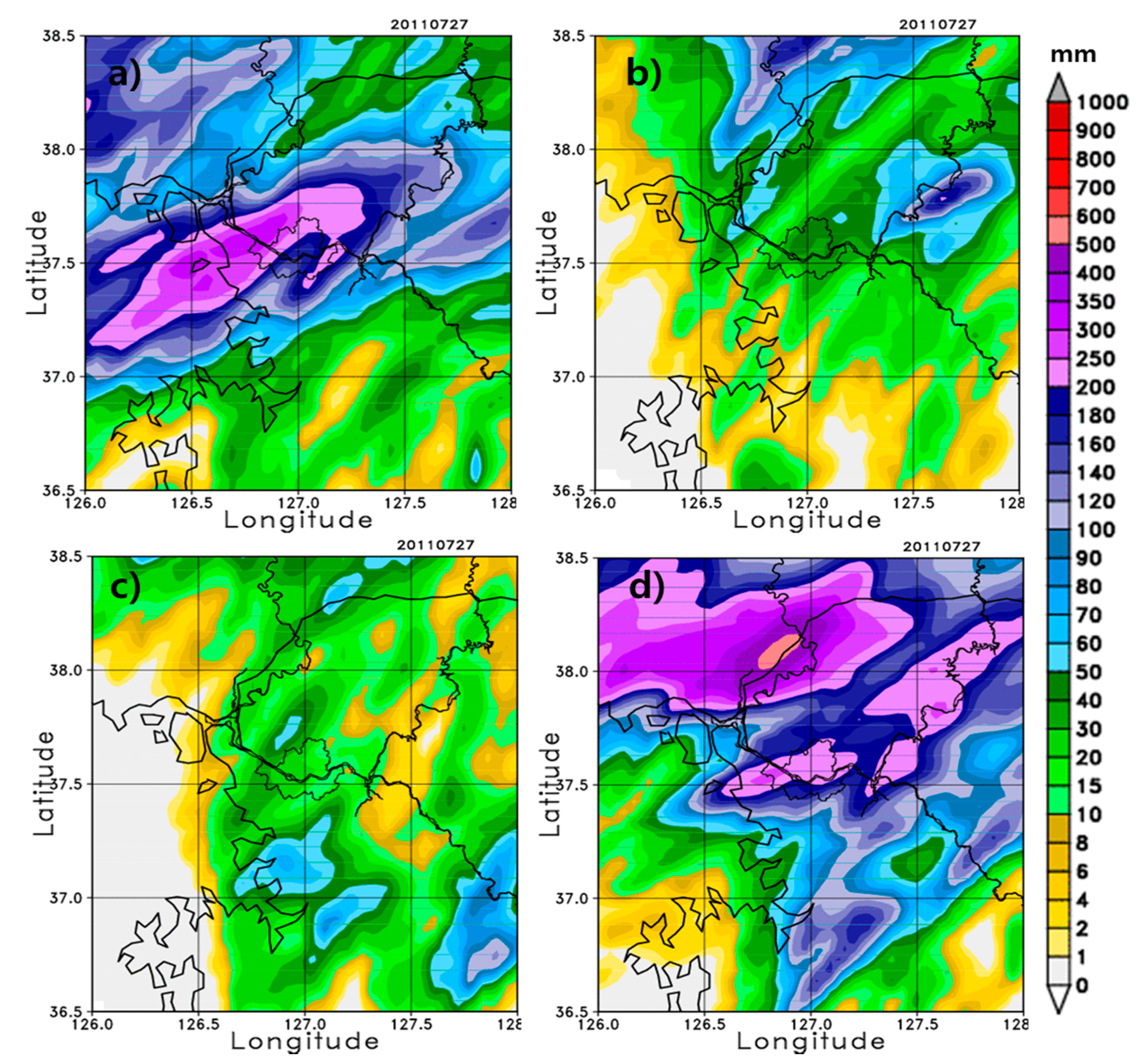
Figure 10.
Lead time effect for the hourly accumulated rainfall at 18 UTC 26 July 2011, starting at (a) 00 UTC 26 July 2011 (+18 h); (b) 06 UTC 26 July 2011; (c) 12 UTC 26 July 2011, which respectively correspond to the lead time effect simulations of +18 h, +12 h, and +06 experiments in Table 2. The color bar represents the rain rate (mm/h). The box in each panel indicates the region bounded by 37.3° N–37.8° N and 126.6° E–127.4° E. See Figure 5a for a comparison to the AWS rainfall analysis.
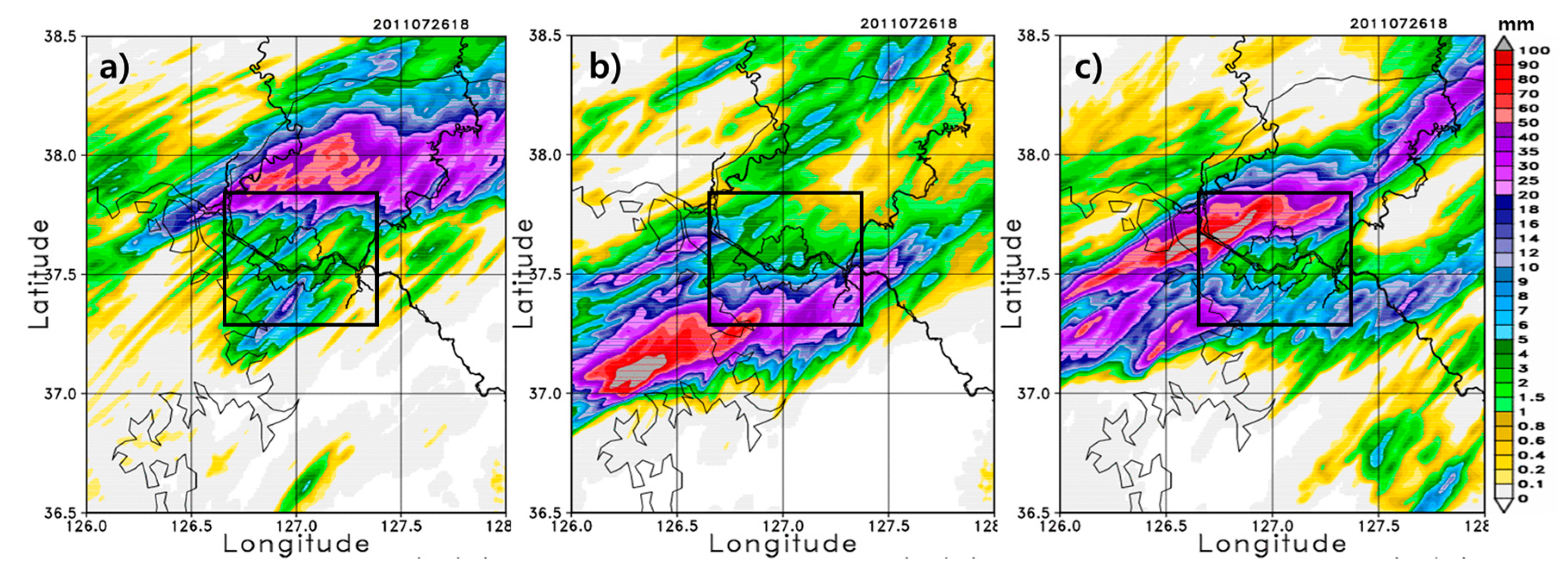
Figure 11.
Domain-averaged hourly rainfall calculated for the region bounded by 37.49° N to 37.8° N latitude and 126.6° E and 127.4° E longitude for the AWS analysis field (black line), default simulation started at 00 UTC (blue line), +12 simulation started at 06 UTC (red line), and +6 simulation started at 12 UTC (sky blue line).


Table 1.
Default model configuration and physical parameterizations.
| Configuration | Outer Domain | Inner Domain |
|---|---|---|
| WRF version | 3.6.1 | |
| Horizontal grids | 332 × 293 | 336 × 286 |
| Grid spacing (km) | 5 | 1 |
| Integration time (s) | 30 | 6 |
| Cumulus | Cumulus Parameterization Scheme (CPS) | N/A |
| Vertical grid | 50 layer/Top 50 hPa | |
| Radiation | Goddard longwave/shortwave scheme; Integration time: 10 min | |
| Microphysics | WRF Single-Moment 6-class | |
| Surface layer | Monin-Obukhov (Janjic) scheme | |
| Land surface | Unified Noah Land Surface Model | |
| Planetary boundary layer | Mellor-Yamada-Jankic turbulent kinetic energy (TKE) scheme; Integration time: 5 min/each time | |
| Initial boundary condition | UM Regional Model Forecast Field (12 km resolution, KMA) | |
| Sea Surface Temperature | Operational Sea Surface Temperature and Sea Ice Analysis (OSTIA) | |
| Land use and topography data | 30s/USGS 33cat | |
Table 2.
Experimental summary for the sensitivity studies of outer domain size, sea surface temperature (SST), initial condition, and lead time. The default model configuration is indicated with a superscript. See the texts in Section 3.2 and Section 3.3 for the acronyms.
Table 2.
Experimental summary for the sensitivity studies of outer domain size, sea surface temperature (SST), initial condition, and lead time. The default model configuration is indicated with a superscript. See the texts in Section 3.2 and Section 3.3 for the acronyms.
| Experiment | Domain Size | SST Data | Initial Condition | Lead Time |
|---|---|---|---|---|
| Simulation 1 default | 0 | OSTIA (5 km) | UMR (12 km) | +18 h |
| Simulation 2 | +150 | RTG-SST (900 m) | UMG (23 km) | +12 h |
| Simulation 3 | +120 | AVHRR (1 km) | ECMWF interim (25 km) | +06 h |
| Simulation 4 | +90 | AVHRR-AMSRE (1 km) | NCEP FNL (100 km) | |
| Simulation 5 | +60 | G1-SST (1 km) | ||
| Simulation 6 | +30 | |||
| Simulation 7 | −30 | |||
| Simulation 8 | −60 |
Table 3.
Summary of the precipitation prediction evaluation indices for sensitivity studies. The threshold value is 0.5 mm/h. POD (Probability of Detection), FAR (False Alarm Ratio), ETS (Equitable Threat Score). Shading indicates the maximum POD and ETS values, and minimum FAR values among simulations for each experiment.
| Domain Size | SST | I/C | Lead Time | |||||||||
|---|---|---|---|---|---|---|---|---|---|---|---|---|
| Simulation | POD | FAR | ETS | POD | FAR | ETS | POD | FAR | ETS | POD | FAR | ETS |
| S1 default | 0.86 | 0.28 | 0.33 | 0.86 | 0.28 | 0.33 | 0.86 | 0.28 | 0.33 | 0.86 | 0.28 | 0.33 |
| S2 | 0.71 | 0.31 | 0.28 | 0.83 | 0.28 | 0.31 | 0.55 | 0.34 | 0.14 | 0.88 | 0.28 | 0.32 |
| S3 | 0.82 | 0.27 | 0.31 | 0.83 | 0.27 | 0.31 | 0.56 | 0.33 | 0.14 | 0.90 | 0.25 | 0.35 |
| S4 | 0.84 | 0.28 | 0.31 | 0.84 | 0.27 | 0.31 | 0.86 | 0.28 | 0.36 | |||
| S5 | 0.84 | 0.28 | 0.32 | |||||||||
| S6 | 0.83 | 0.29 | 0.32 | |||||||||
| S7 | 0.82 | 0.28 | 0.33 | |||||||||
| S8 | 0.85 | 0.29 | 0.34 | |||||||||
Table 4.
Statistical summary for the sensitivity studies. Shading indicates maximum CC, and minimum BIAS and RMSE values among simulations for each experiment.
Table 4.
Statistical summary for the sensitivity studies. Shading indicates maximum CC, and minimum BIAS and RMSE values among simulations for each experiment.
| Domain Size | SST | I/C | Lead Time | ||||||||||
|---|---|---|---|---|---|---|---|---|---|---|---|---|---|
| Variables | CC | BIAS | RMSE | CC | BIAS | RMSE | CC | BIAS | RMSE | CC | BIAS | RMSE | |
| S1 default | T2 | 0.55 | 2.06 | 2.94 | 0.59 | 1.40 | 2.54 | 0.58 | 1.01 | 2.36 | 0.58 | 1.08 | 2.36 |
| WS10 | 0.10 | 2.78 | 3.53 | 0.20 | 2.79 | 3.47 | 0.14 | 2.69 | 3.44 | 0.14 | 2.69 | 3.44 | |
| Rh | 0.12 | −5.43 | 11.04 | 0.23 | −5.13 | 13.08 | 0.17 | −5.68 | 13.22 | 0.17 | −5.68 | 13.22 | |
| S2 | T2 | 0.57 | 2.12 | 2.94 | 0.58 | 2.17 | 3.16 | 0.58 | 1.23 | 2.45 | 0.58 | 1.23 | 2.45 |
| WS10 | 0.15 | 3.35 | 3.87 | 0.13 | 2.74 | 3.35 | 0.10 | 2.57 | 3.76 | 0.10 | 2.57 | 3.35 | |
| Rh | 0.16 | −6.57 | 11.34 | 0.21 | −5.15 | 13.02 | 0.11 | −5.28 | 14.57 | 0.11 | −5.28 | 13.57 | |
| S3 | T2 | 0.56 | 2.06 | 2.88 | 0.58 | 1.79 | 2.82 | 0.43 | 1.89 | 2.92 | 0.59 | 1.28 | 2.42 |
| WS10 | 0.12 | 3.24 | 3.79 | 0.13 | 2.35 | 3.06 | 0.14 | 2.96 | 3.76 | 0.11 | 2.62 | 3.36 | |
| Rh | 0.07 | −6.37 | 12.61 | 0.19 | −5.14 | 13.18 | 0.08 | −6.80 | 13.49 | 0.16 | −5.58 | 13.35 | |
| S4 | T2 | 0.53 | 1.88 | 2.92 | 0.58 | 1.84 | 2.88 | 0.43 | 1.89 | 2.92 | |||
| WS10 | 0.13 | 2.73 | 3.51 | 0.14 | 2.36 | 3.07 | 0.14 | 2.96 | 3.76 | ||||
| Rh | −0.03 | −3.85 | 13.27 | 0.25 | −5.19 | 12.70 | 0.08 | −6.80 | 13.49 | ||||
| S5 | T2 | 0.49 | 1.86 | 3.00 | |||||||||
| WS10 | 0.11 | 2.60 | 3.42 | ||||||||||
| Rh | −0.02 | −4.75 | 12.24 | ||||||||||
| S6 | T2 | 0.54 | 2.22 | 3.05 | |||||||||
| WS10 | 0.12 | 2.32 | 3.16 | ||||||||||
| Rh | 0.05 | −5.61 | 12.91 | ||||||||||
| S7 | T2 | 0.59 | 1.83 | 2.72 | |||||||||
| WS10 | 0.14 | 2.88 | 3.63 | ||||||||||
| Rh | 0.25 | −4.02 | 12.34 | ||||||||||
| S8 | T2 | 0.62 | 1.56 | 2.63 | |||||||||
| WS10 | 0.12 | 3.57 | 4.28 | ||||||||||
| Rh | 0.26 | 2.80 | 15.70 | ||||||||||
© 2017 by the authors. Licensee MDPI, Basel, Switzerland. This article is an open access article distributed under the terms and conditions of the Creative Commons Attribution (CC BY) license (http://creativecommons.org/licenses/by/4.0/).
Share and Cite
MDPI and ACS Style
Jee, J.-B.; Kim, S. Sensitivity Study on High-Resolution WRF Precipitation Forecast for a Heavy Rainfall Event. Atmosphere 2017, 8, 96. https://doi.org/10.3390/atmos8060096
AMA Style
Jee J-B, Kim S. Sensitivity Study on High-Resolution WRF Precipitation Forecast for a Heavy Rainfall Event. Atmosphere. 2017; 8(6):96. https://doi.org/10.3390/atmos8060096
Chicago/Turabian StyleJee, Joon-Bum, and Sangil Kim. 2017. "Sensitivity Study on High-Resolution WRF Precipitation Forecast for a Heavy Rainfall Event" Atmosphere 8, no. 6: 96. https://doi.org/10.3390/atmos8060096
Note that from the first issue of 2016, this journal uses article numbers instead of page numbers. See further details here.