Research on the Fine-Scale Spatial Uniformity of Natural Rainfall and Rainfall from a Rainfall Simulator with a Rotary Platform (RSRP)

Abstract

The accurate production of a rainfall environment similar to natural rainfall by a rainfall simulator (RS) is a crucial and challenging task in rainfall instrument testing or calibration. Although the spatial uniformity of rainfall accumulation is a key parameter of an RS, the spatial uniformity comparison between simulated rainfall and natural rainfall, and the spatial uniformity improvements for an RS are scant in the literature. In this study, a fine-scale natural rainfall experiment was studied using the same testing methods of an RS and the rainfall uniformity was evaluated using the Christiansen Uniformity Coefficient (CU). Simultaneously, factors influencing the spatial uniformity of natural rainfall, including the average rainfall accumulation (RA), the deviation of RA, and the area of the test zone, were analyzed. The results successfully reproduced some of the behaviors observed in natural rainfall experiments, showing that CU is dependent on these parameters. Based on these studies, we developed a rainfall simulator with a rotary platform (RSRP) and found that although spatial uniformity of the RSRP was greatly improved using an appropriate rotary speed, it was not consistent with the spatial uniformity of natural rainfall. Furthermore, we tested four tipping-bucket rain gauges using this imperfect RSRP, and found that the RSRP might acquire the instrumental errors associated with RA for a tested rainfall instrument.

1. Introduction

A rainfall simulator (RS) that can produce a controllable rainfall environment similar to natural rainfall is important for studying soil erosion, soil hydrological processes, and rainfall instrument testing or calibration, and can save time compared to testing during natural rainfall events [1,2]. However, obtaining an accurate rainfall environment consistent with naturally-occurring rainfall events remains a challenge, mainly because of the complexity of the micro-physical variables of rainfall characteristics and the heterogeneity of natural rainfall [3,4,5].

At present, there are two types of RSs; the first is the nozzle type, which produces rain of very high intensity and a wide range of rainfall drops that tend to give lower overall uniformity, and the other is the needle type, which produces higher uniformity but is used when one needs to simulate rain to fall from a height of 5 m or more [6,7]. Colli et al. [8] designed and conducted preliminary tests of an advanced needle-type laboratory RS capable of generating discontinuous droplets with a controlled rainfall intensity and drop size distribution (DSD), but it was difficult to produce drops with a diameter less than 1.5 mm. Furthermore, it was quite difficult to ensure that the velocity of the artificial raindrops was consistent with that of natural raindrops. In order to solve these problems, Liu et al. [9] designed a nozzle-type RS prototype, and evaluated it with the Christiansen Uniformity Coefficient (CU), whose values ranged from 80.12–87.32%.

Although a number of previous RS studies considered a CU of 80% or greater to be sufficient to ensure realistic simulated rainfall patterns [10,11], the CU values of the current RS were too low to apply to rainfall instrument testing or calibration compared to natural rainfall uniformity exceeding 95% [12]. In addition, the uniformity improvements of RS are an urgent problem for rainfall instrument testing or calibration.

Although an RS can offer a rainfall environment for testing rainfall instruments, one should be aware of the discrepancies between artificial and natural rainfall. The purpose of the present study is to investigate the consistency of the spatial uniformity between simulated rainfall and natural rainfall. Thus, it attempts to quantify the spatial uniformity of natural rainfall events with CU, improve the spatial uniformity of the RS with a rotary platform to match natural rainfall scenarios, and address the factors affecting the CU value.

This study is organized as follows: Section 2 provides a brief introduction to the rainfall simulator with a rotary platform (RSRP) and quantifies the spatial uniformity of natural rainfall, followed by an analysis of the factors influencing it; Section 3 analyzes the spatial uniformity of rainfall produced by the RSRP (tipping-bucket rain gauge (TBRG) tests with the RSRP are presented here) and discusses the results; finally, Section 4 summarizes and concludes the paper.

2. Experiments

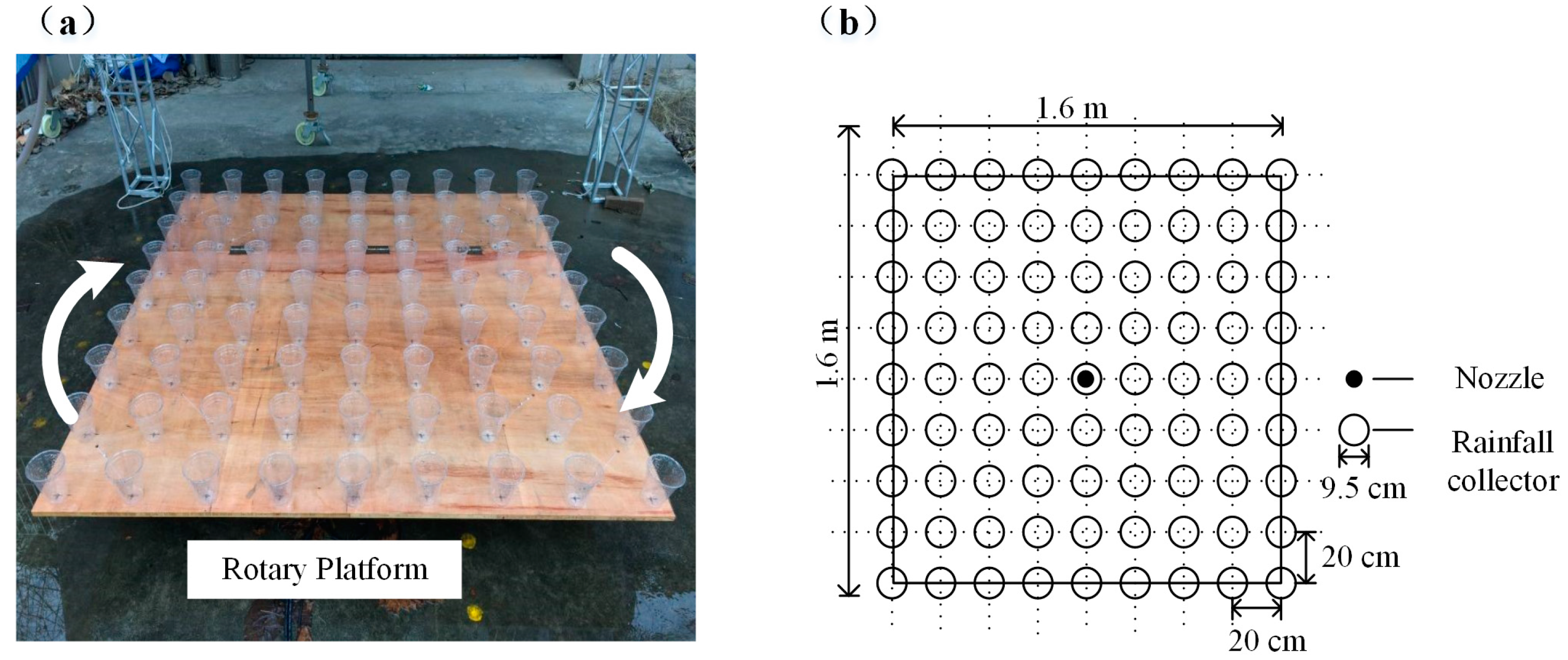
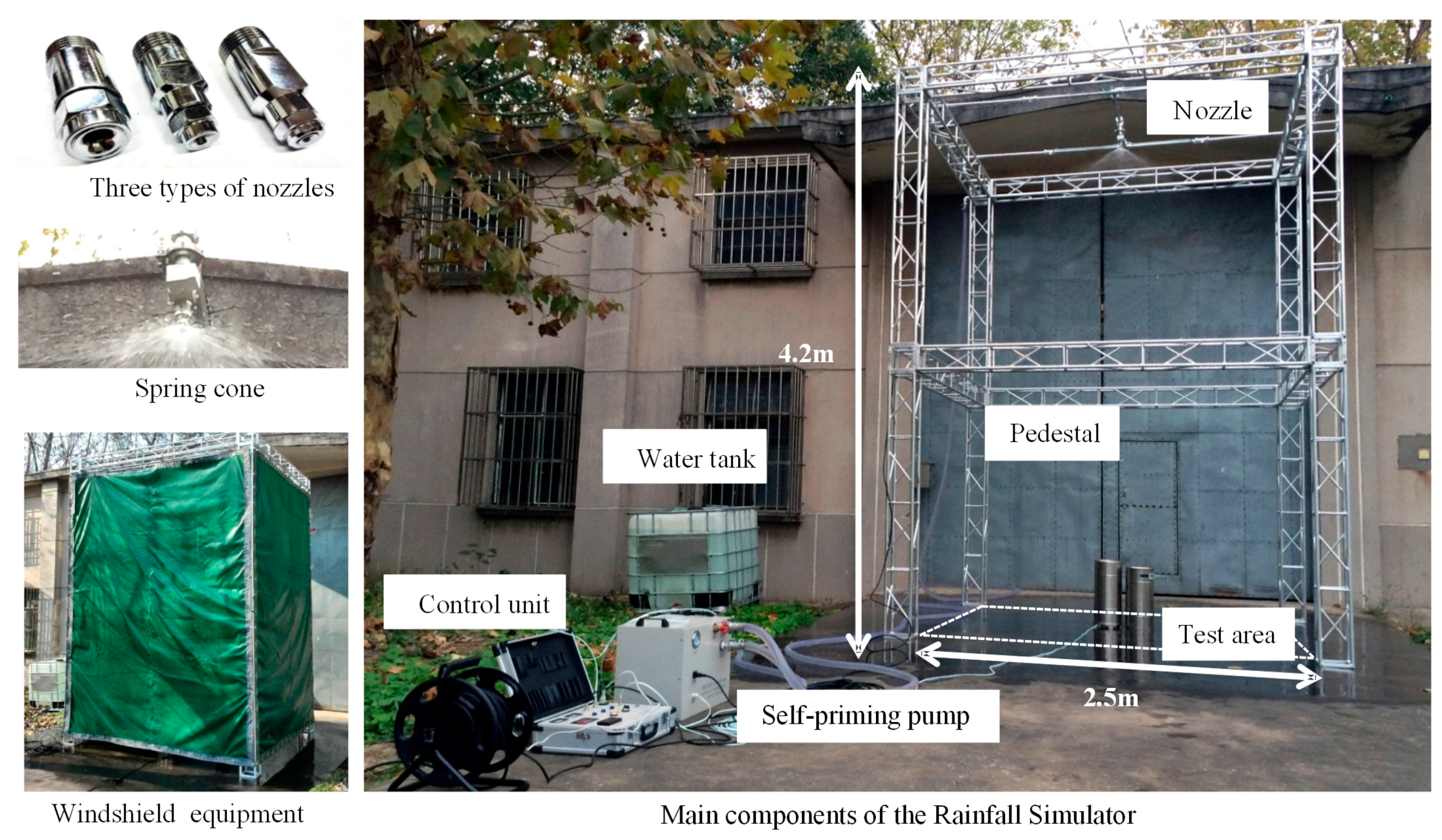
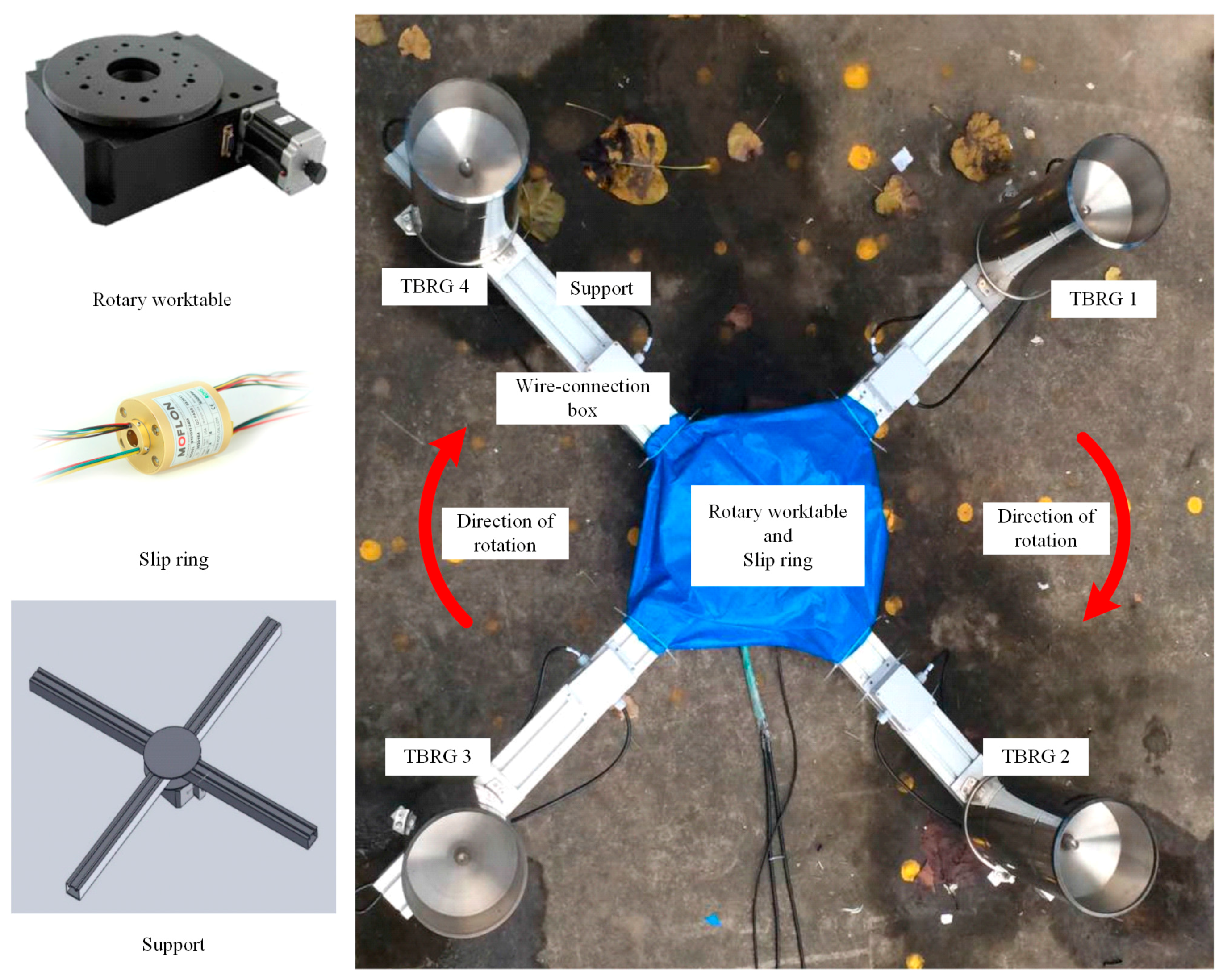
2.1. Rainfall Simulator with a Rotary Platform (RSRP)

Two different methods are used to improve the spatial uniformity of a rainfall simulator: a rotating nozzle mechanism and a rotating platform mechanism [13,14,15]. The main difference between these two methods is that the former is used to improve the uniformity of the rainfall environment, while the latter is used to improve the relative uniformity. As the latter one was more practical to adopt for this study, we adopted it to improve the spatial uniformity of our RS.

The RSRP comprises a rotary platform placed below the nozzle of a rainfall simulator. Both catching rain gauges and non-catching rain gauges can be located on the support of the rotary worktable, which would rotate with the test platform under the laboratory rainfall simulator. An uninterrupted power supply and signal transmission during rotation is a key requirement of the RSRP. We incorporated a slip ring to ensure that this requirement is met.

The RS, the main part of the RSRP, is a single nozzle-type rainfall simulator. It consists of a nozzle, pedestal, water supply system, control box, and windshield equipment (Figure 1). An aluminum alloy pedestal was built to hold the nozzle 6 m above the ground to simulate a more realistic velocity [16,17]. The produced rainfall intensity can be varied between 8 mm/h to 40 mm/h by adjusting the pressure at the nozzle inlet. The present experiment was undertaken with a full cone jetting-type nozzle (HH-14W, Spraying System Co., Wheaton, IL, USA). The operating pressure is 0.07 MPa and the specific spray cone angle is 120°. A self-priming pump, with a power consumption of 1.2 kW, drew water from a 1 m³ water tank to the nozzle inlet. To control the beginning and ending of the simulated rainfall, a solenoid valve was added to at its point of entry to the nozzle. The solenoid valve opened when it was energized by a 12 V electric current, which was operated by the control box. The response speed of the solenoid valve was fast enough to prevent the nozzle from dripping after the valve was shut. A pressure gauge located between the pressure regulator and nozzle was used to monitor pressure during tests. Pressure values were within ±1 kPa of the nominal pressure rating [9].

The rotary platform consists of a rotary worktable, slip ring, support, and four wire-connection boxes. The test platform is driven by the rotary worktable, and the rainfall measuring data are transmitted through the slip ring and wire connection boxes. Figure 2 shows the rotary platform and main components.

The rotary worktable is an electrical rotary table with a high absolute positioning accuracy of 0.005°, worm gear, and worm mechanism. The weight of the center can be up to 100 kg. Each step of the stepper motor is 1.8° with a total scope of 360° and an idling speed is 25°/s. The slip ring (MT012 standard series, MOFLON Technology Co., LTD, Shenzhen, China) has a total of 24 signals, including 18 signals of 2 A and six signals of 10 A. It can provide six signals, allowing the rainfall instrument to be tested in each direction. During the experiment, the tested rainfall instruments included the TBRG with only two signals and an optical disdrometer with four signals. The wire-connection box combines the tested instruments with the slip ring, and the slip ring is attached to the data acquisition system. For the TBRG, we developed a four channel data acquisition (DAQ) system based on LabVIEW (Laboratory Virtual Instrument Engineering Workbench), which saves the information to a .txt file every minute. The employed tipping buckets have collection funnels of 20 cm in diameter to redirect the collected rainfall to one of the buckets at a time.

The rotary platform is connected to the controller and can be started or stopped by the start and stop buttons on the controller. The rotary speed and rotary angle can be burned to the controller on the computer. The rotary platform is initiated using a slow start and slow stop mechanism; when the speed of the test platform changes, the controller must be reprogrammed and reburned to the controller.

2.2. Quantification of the Spatial Uniformity of Natural Rainfall and Analysis of Influencing Factors

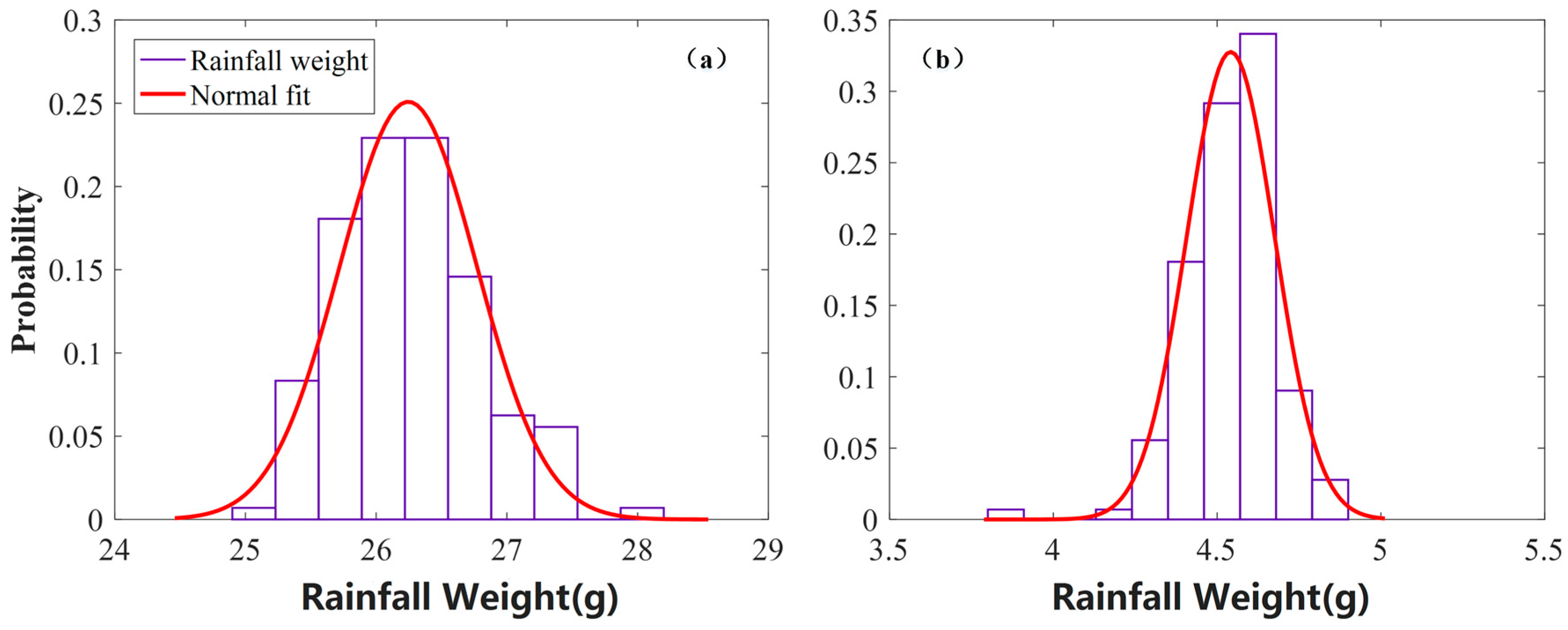
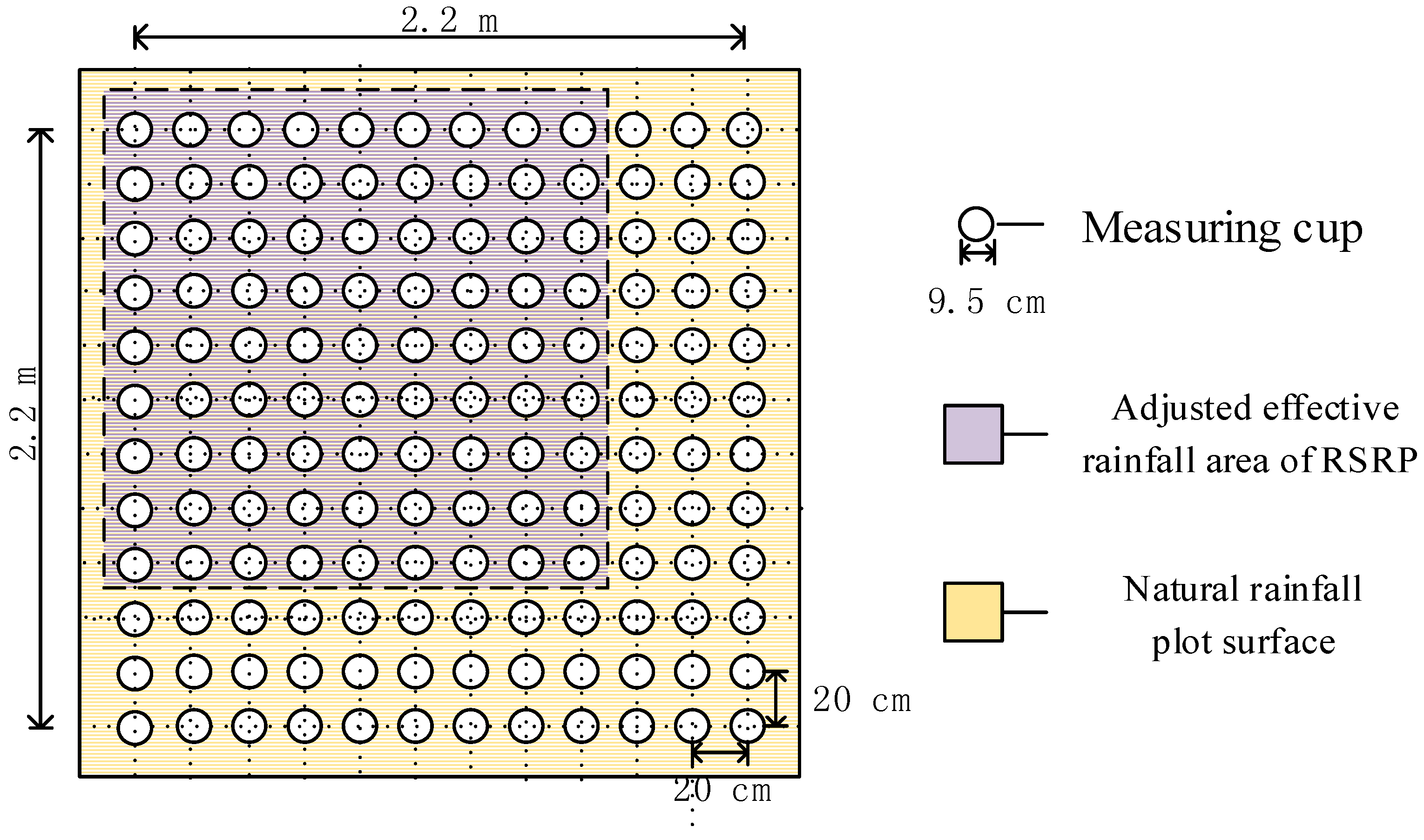
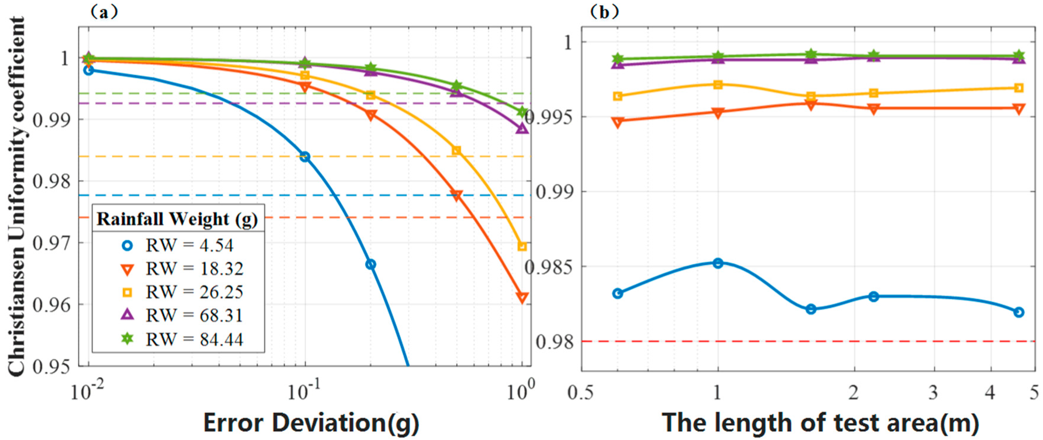
2.2.1. Quantification of the Spatial Uniformity of Natural Rainfall

A number of previous rainfall simulation studies considered a Christiansen Uniformity Coefficient (CU) of 80% or greater to be sufficient to ensure simulated rainfall patterns are realistic, while CU values of above 62% have been accepted in other studies for larger plot areas. Thus, it is necessary to obtain CU values in the natural rainfall events [12]. Additionally, the test area and the test conditions may be factors affecting the CU values. Therefore, an experiment was conducted under natural rainfall to quantify its uniformity with the same scale of the RS and to determine to what degree the RS should be set.

In order to characterize the spatial rainfall distribution in naturally-occurring rainfall events, 144 circular measuring cups of 9.5 cm diameter and 10.8 cm height were evenly distributed on the entire test plot (2.2 m × 2.2 m, 4.84 m²). The test area size was chosen to represent the intended test area of the RS as closely as possible. The center-to-center distance between the measuring cups was 20 cm (Figure 3). A thin layer of sponge was used to cover the board to reduce the splashing error.

Considering the effect of wind and the convenience of measurement, two measuring cups were stacked at every measuring point. One of them was nailed to the board, while the other was used for measurement. In order to avoid other environmental conditions from affecting the experiment, an oil cloth was used to cover the measuring cups during periods of no rainfall. Before the rainfall started, the cover was removed to expose the empty measuring cups to natural rainfall for the duration of the event. Once the rainfall ceased, every individual cup was weighed by a precision electronic balance of 0.01 g, recording the rainfall accumulation at each position. Here, we hypothesized that there was no evaporation loss out of the open collectors during the experiment, but we should consider that in the future experiments.

The rainfall accumulation values were calculated using Equation (1), which transformed the weight into volume. RA represents the rainfall accumulation at an individual test point within a period, m denotes the weight of a measuring cup with rainfall inside in grams, while m₀ represents the weight of an empty measuring cup. Additionally, $\rho$ represents the density of water in g/cm³ and $A$ represents the area of the measuring cup at the inner top edge in cm². The diameter of the area is measured using a Vernier caliper with an accuracy of 0.02 mm.

$$RA=\frac{\left(m-m_0\right)}{\rho \times A}\times 10$$

(1)

To account for the different weights of each measuring cup, all of the cups were marked from 1 to 144, and weighed using the balance to obtain m₀. The average m₀ was 10.58 g, while the standard deviation was 0.17 g. An OTT PARSIVEL optical disdrometer (OTT Hydromet GmbH, Kempten, Germany) [18] was deployed beside the test plot to record the beginning and ending times of the natural rainfall events.

The most widely used coefficient of uniformity for a tested rainfall zone was defined by Christiansen [19], as shown in Equation (2). CU, the Christiansen Uniformity Coefficient of rainfall accumulation, is an important index to be considered in the design of a functional and accurate RS [12]. RA_i represents the rainfall accumulation (mm) of the current cup number i. n is the number of the testing cups (equal to 144 in this experiment).

$$CU=\left(1-\frac{{\displaystyle \sum _{i=1}^n\left|R{A}_i-\overline{RA}\right|}}{n\overline{RA}}\right)\times 100\%$$

(2)

We hypothesized that the diameter differences in the measurements of the measuring cup were very little, so we used the average diameter and area to represent each measuring cup. By combining with Equations (1) and (2), we obtain Equation (3). In Equation (3), $\mathsf{\Delta }m$ was calculated by subtracting m₀ from m. For this reason, we can use the rainfall weight to represent the rainfall accumulation in the discussion.

$$CU=\left(1-\frac{{\displaystyle \sum _{i=1}^n\left|(\mathsf{\Delta }{m}_i)-\overline{\mathsf{\Delta }m}\right|}}{n\overline{\mathsf{\Delta }m}}\right)\times 100\%$$

(3)

The rainfall event data used in this study were collected at a weather station in Nanjing, China, from December 2015 to January 2016. To get a basic understanding of these five referred rainfall events, the average rainfall weight, standard deviation of the rainfall weight, the ratio of the former two parameters, and the CU values over the entire test area are presented in

Table 1. Uniformity test results of five natural occurring rainfall events with the scale of 2.2 m × 2.2 m. $\overline{\mathsf{\Delta }m}$ corresponds to the average rain weight of all 144 measuring points and σ refers to the standard deviation of the referred differences.

Rainfall Events	Date	Duration (h)	$\overline{\mathsf{\Delta }\mathit{m}}$ (g)	RA (mm)	σ (g)	$\frac{\mathsf{\sigma }}{\overline{\mathsf{\Delta }\mathit{m}}}$	CU
No.1	2015.12.02	4.5	26.25	3.70	0.52	0.0198	98.40%
No.2	2015.12.05	3.2	4.54	0.64	0.13	0.0286	97.77%
No.3	2016.01.03	34.4	84.44	11.91	0.61	0.0072	99.42%
No.4	2016.01.08	12.7	68.31	9.64	0.59	0.0086	99.26%
No.5	2016.01.15	8.6	18.32	2.58	0.51	0.0278	97.41%

. From the table, we can obviously conclude that the CU of naturally-occurring rainfall events with the scale of 2.2 m × 2.2 m are greater than 97%, and the maximum CU reaches 99.42%. Similar results were found by [12] when measuring an area of 0.99 m × 2.145 m. In their experiment, the maximum and minimum CU values were 98.4% and 95.1%, respectively, which were slightly lower than those for the current experiment. Thus, whether the scale of the test area could be a possible source of error to this difference would be discussed later.

Table 1 shows that the increased average rainfall weight improves the standard deviation of the rainfall weight, but the opposite trend is observed for $\mathsf{\sigma }$/$\overline{\mathsf{\Delta }m}$, except for event No. 5. Although the overall tendency of CU is to increase with increasing average rainfall weight, it is still difficult to draw this conclusion because the number of rainfall events is small. Thus, more events should be evaluated in future studies on the relationship between RA and CU.

In order to quantify CU at the 1.6 m × 1.6 m scale, we analyzed 16 test areas of 1.6 m × 1.6 m within the 2.2 m × 2.2 m area using rainfall events No. 1 and No. 2. The mean CU of event No. 1 was 98.37%, and the standard deviation was 0.05%, while the corresponding values for event No. 2 were 98.19% and 0.33%, respectively. It is quite apparent that CU of naturally-occurring rainfall events at the 1.6 m × 1.6 m scale is greater than 98%, which indicates that the RS must at least meet this level.

2.2.2. Analysis of Factors Influencing Spatial Uniformity of Natural Rainfall

To determine the factors that influence the spatial uniformity of natural rainfall, the possible sources contributing to errors in CU were analyzed. Two aspects were considered to evaluate the discrepancies in CU. The first is that the spatial heterogeneity of natural rainfall seems to exist on a scale of centimeters [20,21]. The other refers to the observation error, including instrumental effects [22,23]. All of these possible errors could result in discrepancies among CU values and, thus, we assumed that the error deviation of the rainfall weight represents the summation of all of the possible errors mentioned above. In order to evaluate the errors in the observed CU data, we referred to Equation (3) and found that three parameters could affect CU. They were average RA ($\overline{\mathsf{\Delta }m}$), deviation of RA ($(\mathsf{\Delta }{m}_i)-\overline{\mathsf{\Delta }m}$), and the area of the test zone (n). Next, we studied how these three aspects affected the estimation of CU by means of a simulation analysis.

Before the simulation, we plotted the statistical distribution of rainfall weight based on natural rainfall events No. 1 and No. 2, and fitted a normal distribution. The fitted distribution and histogram plots for these two events are displayed in Figure 4, which shows that the normal distribution can be used to describe the variability of the natural rainfall events.

The simulation comprised three steps. First, we set the parameters of the tested area, such as the error deviation of the rainfall weight, length of the tested area, and mean rainfall weight, which described a basic rainfall event. Second, we used the normal distribution to simulate the variability, adding the deviation to the average values, to obtain all rainfall accumulations in the test area. Finally, we changed one of the three parameters and calculated CU.

Figure 5 shows how these three factors influence CU. The five rainfall weights were chosen from Table 1. As the accuracy of the precision electronic balance is 0.01 g, we used 0.01 g as the minimum error. Reexamining Table 1 showed that the maximum deviation is 0.61 g; thus, we used 1.0 g as the maximum error, and the other three errors were set at 0.1 g, 0.2 g, and 0.5 g. From Figure 5a, it is obvious that increasing the error deviation decreases the uniformity, and lower rainfall weights are more likely to be influenced by the error deviation, especially if the error deviation exceeds 0.2 g. Combining the simulated CU values with the tested CU values at certain rainfall weights, we found the intersections are at 0.13 g, 0.60g, 0.53g, 0.69 g, and 0.60 g. A comparison of these values with the two values of σ in Table 1 showed that perfect consistency at rainfall weights of 4.54 g, 26.25 g, and 88.44 g, but the remaining two values of σ are within 0.1 g. The results are quite convincing, and show that it is prudent to control the error deviation to within 0.2 g. Figure 5b reveals that the CU values of the test areas are not related, and we noted that when the rainfall weight exceeds 4.54 g, CU is greater than 99.5%.

While the simple approximation of the error deviation of rainfall weight is useful, further research on detailed error deviations is required. As the uniformity evaluation at every test point uses a catching-type gauge, the CU might be affected by the dynamic pressure fluctuations generated by wind over the orifice of the rain gauge (the wind pumping effect), and the temperature and humidity of the air [24]. Constant pressure and discharge can be maintained by a hydraulic system, and the wind-induced error in CU can be studied experimentally with wind sensors or numerically simulated with a computational fluid dynamics (CFD) approach [25]. In addition, it is important to check whether the inhomogeneity of rainfall accumulation influences the results of field comparisons.

3. Results and Discussion

To determine the spatial uniformity improvements with the RSRP, two experiments were conducted. First, the spatial uniformity was evaluated with measuring cups to investigate the discrepancy between artificial rainfall and natural rainfall. Second, the TBRGs were tested in the RSRP to examine the possibility of applying it to rainfall instrument testing or calibration.

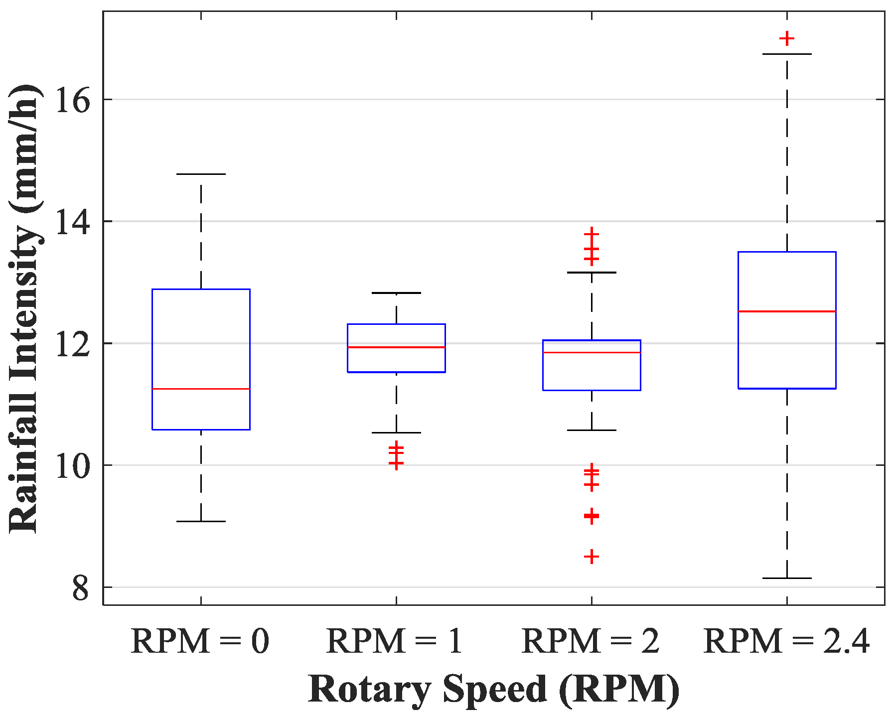
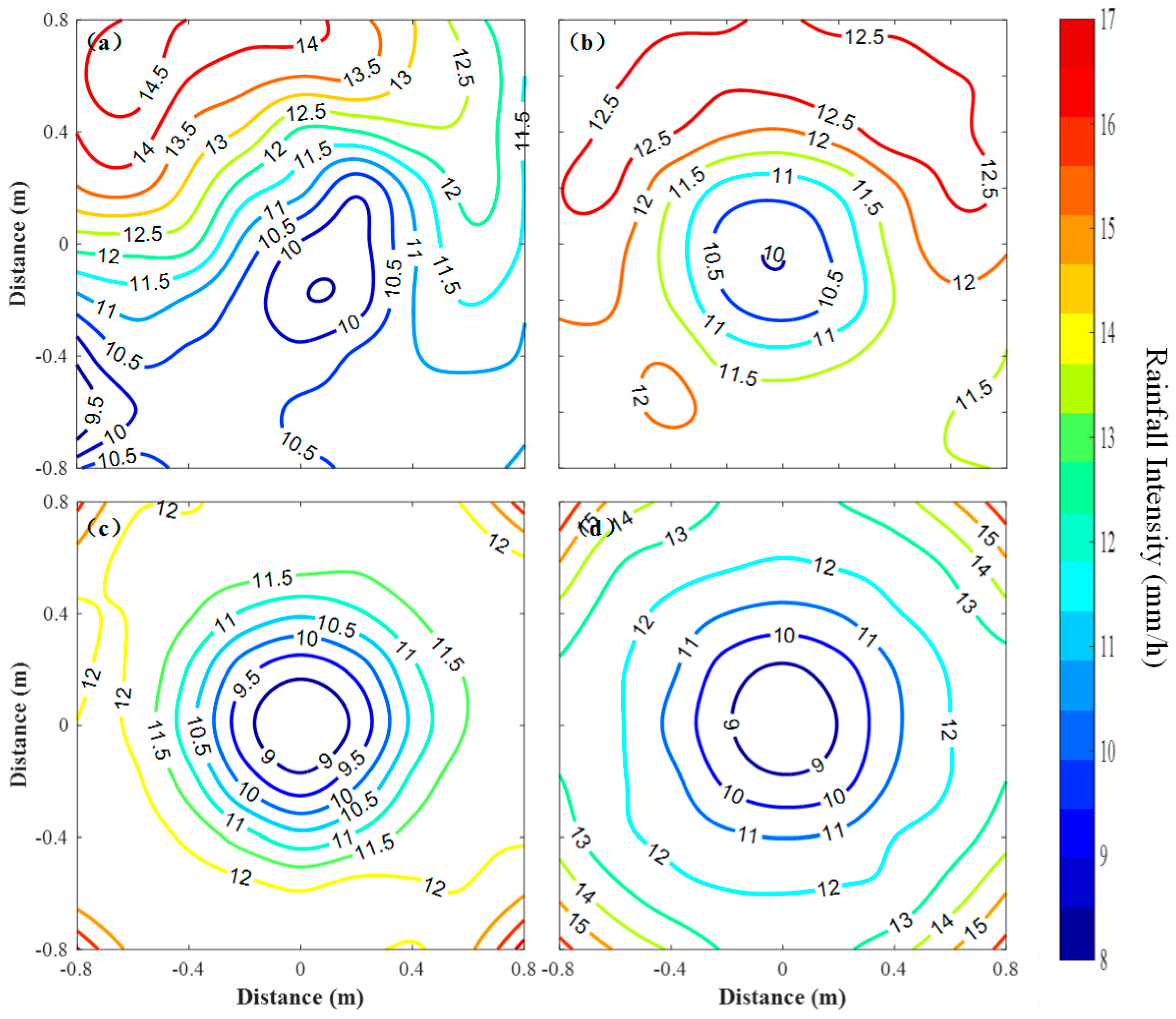
3.1. Spatial Uniformity Evaluation of the Rainfall Simulator with a Rotary Platform

Due to the rotation of the test platform, the maximum length of the test area was determined using the formula $d\le \raisebox{1ex}{$2.5$}\!\left/ \!\raisebox{-1ex}{$\sqrt{2}$}\right.=1.77$ m. The adjusted effective rainfall area (AERA) was adjusted to 1.6 m × 1.6 m to make efficient use of the rainfall field. In order to quantify the uniformity of the RS, 81 measuring cups were distributed evenly on a board with a 0.2 m spacing between each cup, as shown in Figure 6. During the experiment, the board was put on the rotary platform and rotated. The arrows in Figure 6a indicate the direction of rotation.

As the rotary speed is influenced by the weight on the test platform, we conducted several tests with the platform and found that the maximum rotary speed was up to three revolutions per minute (RPM) for the above TBRGs (Figure 2), and the speed was reduced to 2.4 with the uniformity test platform. The uniformity experiments were performed at the following rotary speeds: 0, 1, 2, and 2.4 RPM. The duration of each test was exactly 20 min. The rainfall accumulations were spatially interpolated by the cubic spline interpolation method to obtain a contour map, and CU was used to evaluate the uniformity of the RS.

The artificial rainfall contour maps for the rotary speeds 0, 1, 2, and 2.4 RPM are shown in Figure 7. At the rotary speed of 0 RPM, namely the original state of the RS without rotation, the contour lines are divergent and do not form a closed contour. With an increase in rotary speed, the number of rainfall intensity isolines increase, and the rainfall intensity isoline map takes the shape of a valley, wherein the minimum rainfall intensity occurs in the area under the nozzle, increasing from the middle to the surrounding areas. This trend may be attributed to the outlet pressure of the nozzle being too low to allow the raindrops to completely disperse; the large raindrops are mostly distributed in the corners. The spatial uniformity can be improved by reducing the test area.

In addition to the study of the rainfall intensities contour maps in rotary state, a statistical analysis [26] of the rainfall intensities values for each rotary speed provides a better insight and can address significant differences between rotary speeds. Figure 8 shows the boxplots for each rotary speed. The distribution of rainfall intensities narrows in 1 RPM and 2 RPM, proving that our setup improves the results in general.

In order to quantify the spatial uniformity in the test areas, two additional test areas of 1.2 m × 1.2 m and 0.8 m × 0.8 m were selected to compare with the entire area of 1.6 m × 1.6 m. The results are shown in

Table 2. Summary of the test results indicating the influence of rotary speed and the test area on CU and the maximum deviation of rainfall weight. The maximum deviation of rainfall weight refers to the difference between the maximum rainfall weight and the minimum rainfall weight of all 81 measuring points.

Rotary Speed	CU			The Maximum Deviation of Rainfall Weight (G)
(RPM)	1.6 × 1.6 (m)	1.2 × 1.2 (m)	0.8 × 0.8 (m)	1.6 × 1.6 (m)	1.2 × 1.2 (m)	0.8 × 0.8 (m)
0	89.43%	90.06%	92.24%	13.45	12.36	9.11
1	95.87%	95.09%	94.81%	6.59	6.59	6.43
2	94.00%	92.82%	92.39%	12.48	8.84	8.01
2.4	89.26%	91.00%	91.19%	20.91	12.57	9.08

. An increase in rotary speed from 0 to 2.4 RPM first increases CU, and then decreases it. Different speeds present different trends when the test area decreases. Regarding the maximum deviation of rainfall weight, the influence of rotary speed has the same trend as that for CU, but the different tendency with respect to the test areas can be explained by the fact that the maximum rainfall weight was recorded in the corners.

A possible explanation for these results is that the rotary platform is equivalent to the existing wind above the measurement instrument, with 1 RPM at a radius of 0.8 m referred to as $1\times 2\pi ÷60\times 0.8=0.084$ (m/s). As the relative wind speed is too low, we were uncertain whether the wind is the main cause. It is apparent, however, that the rotary speed of the test platform should be set at a limited value. Reexamining Table 2 showed that when the rotary speed is 1 RPM and the test area is 1.6 m × 1.6 m or 1.2 m × 1.2 m, the uniformity of the RS is maximized or greater than 95%. Therefore, we considered 1 RPM as the most appropriate rotary speed for the rotary platform. Furthermore, if we could obtain a nozzle with a higher uniformity, we would obtain higher CU values by using the rotary platform.

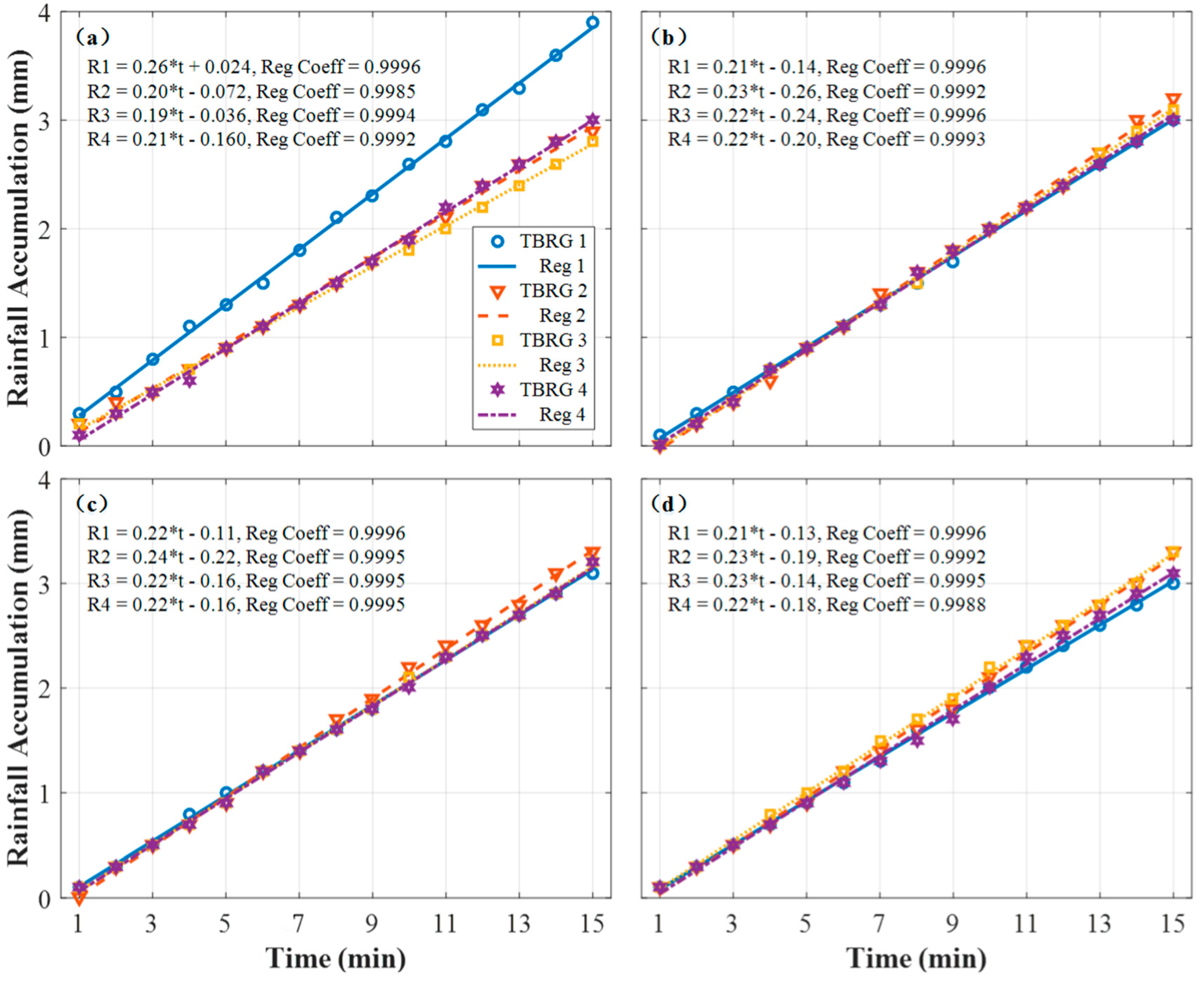
3.2. TBRG Tests of the Rainfall Simulator with a Rotary Platform

Before the TBRGs were tested in the RSRP, the TBRGs were tested under a flow-type rainfall intensity standard device that is widely used as a calibration tool for catching rain gauges. The flow rate of the standard device was set at 6.28 mL/min, and the volume was set at 94.2 mL for a 200 cm diameter bucket. The average test results of rainfall intensity (RI) and RA were 12 mm/h (0.2 mm/min) and 3.0 mm, respectively. Every TBRG was tested thrice, and the results are shown in

Table 3. Measurement accuracy of tipping-bucket rain gauges (TBRGs) assessed over three trials under the laboratory flow-type rainfall intensity standard device testing. 1st, 2nd, and 3rd refer to the measurement time series.

Number	RA (mm)			Average RA (mm)
	1st	2nd	3rd
TBRG 1	3.1	3.1	3.0	3.1
TBRG 2	3.2	3.2	3.1	3.2
TBRG 3	3.3	3.2	3.2	3.2
TBRG 4	3.1	3.1	3.1	3.1

. The table indicates that the mean RA of TBRG 2 and TBRG 3 is greater than those of TBRG 1 and TBRG 4. The RI (mm/min or mm/h) was calculated using Equation (4), with t represents the time of the $RA$:

$$RI=\frac{RA}{t}$$

(4)

Although the CU of the RSRP (95%) is not as high as that of naturally occurring rainfall (98%), four TBRGs were distributed at the same distance (0.8 m to the center of rotary platform) on the support arms in the RSRP (Figure 2) to determine if the discrepancy between TBRGs could be found in the experiments. The experiments were performed for durations of 15 min and at rotary speeds of 0, 1, 2, and 3 RPM. The results are shown in Figure 9. Compared with the stationary state (0 RPM), the RA consistency of the four TBRGs was better during the rotating state (1, 2, or 3 RPM).

As noted in Section 2.2.2, there are two possible explanations for the discrepancies in the TBRGs at the same length of the rotary arm. The first is the spatial inhomogeneity of artificial rainfall, and the other is the instrumental error of the TBRGs. When the speed of the test platform was set at 0 RPM, both aspects contributed to the bias. When the test platform was rotated, the bias of the environment decreased and, thus, the discrepancies among the TBRGs mainly depend on instrumental error. By examining Figure 8, it becomes apparent that the rotary platform improves the RA agreement among the four tested TBRGs.

In order to have a clear understanding of the improvements to the RA and RI, we summarize the statistical results of RA and RI for the TBRGs. The results are shown in

Table 4. The statistical results of RA and RI for the tipping-bucket rain gauge (TBRGs) tests with four selected rotary speeds. The maximum RA bias is the difference between the maximum RA of the four tested TBRGs and the minimum RA at a certain rotary speed. The consistent numbers of RI value are the numbers of the same RI value in every minute among the four TBRGs within 15 min.

Rotary Speed (RPM)	RA (mm)				The Maximum RA Bias (mm)	Consistent RI Values
	TBRG 1	TBRG 2	TBRG 3	TBRG 4
0	3.9	2.9	2.8	3.0	1.1	3
1	3.0	3.2	3.1	3.0	0.2	6
2	3.1	3.3	3.2	3.2	0.2	6
3	3.0	3.3	3.3	3.1	0.3	8

. The table shows that the maximum bias for RA drops from 1.1 mm to 0.2 mm when the platform rotates, as the rotary platform enhances the distribution of the artificial rainfall. Furthermore, the numbers for the same RI values show an obvious increase for every minute. When the rotary speed is set at 3 RPM, however, the maximum RA bias is larger than that at 2 RPM. This shows that the speed of the rotating test platform should not be increased excessively. Therefore, it can be concluded from Table 4 that the best rotary speed for the RSRP is either 1 or 2 RPM, as noted in Section 3.1.

Furthermore, when we subtracted the average TBRG RA under the laboratory testing device from the TBRG RA under the RSRP at a speed of 1 RPM (E_RSRP1), we obtained the environmental error of RA from the RSRP (E_E = E_RSRP1 − E_L1). E_L1 was assumed to be the RA measurement error of the No. 1 rainfall instrument at the same testing condition with the RSRP experiments. The environmental errors of the four test positions are −0.1 mm, 0 mm, −0.1 mm, and −0.1 mm, respectively. Therefore, we can change the tested rainfall instruments (No. 2) of the referenced test points and can obtain the instrumental errors within the above-mentioned RI and RA values (E_L2 = E_RSRP2 − E_E, E_L2 and E_RSRP2 are the No. 2 rainfall instrument‘s error and its testing result under the RSRP, respectively). Unfortunately, we missed recording the test result of rainfall instrument No. 2. In any event, the spatial uniformity improvements in the RSRP are very promising. However, much work remains to be done in the future before applying the RSRP in the field for rainfall instrument testing or calibration.

4. Conclusions

We measured the rainfall accumulation uniformity of naturally occurring rainfall within a 2.2 m × 2.2 m area using 144 measuring cups. Five rainfall events were recorded, and the CU were used to evaluate the rainfall distribution. The uniformity analysis of a 1.6 m × 1.6 m area indicated that the CU values of the RS under development should match the CU values of natural rainfall events. Furthermore, we analyzed the influencing factors of spatial uniformity in natural rainfall, including average RA, error deviations, and test areas. We concluded that the limit of the error should be less than 0.2 g in order to obtain a CU value above 99%; the test area had a weak relationship with CU. Notably, these findings are applicable to both RS and natural rainfall when the statistical RA measurements are fitted with a normal distribution.

In addition, we developed an RSRP to study the spatial uniformity improvements at different rotary speeds. We concluded that the spatial distribution of RA for the RS noticeably improved when the rotary platform was rotated. Similar results were observed for the TBRGs; however, the CU of the current RSRP is still somewhat low compared with natural rainfall. Although the spatial uniformity improvements of the RSRP are very obvious, more work, including considering additional RAs and using a constant hydraulic system, should be conducted in the future to implement rainfall instrument calibration or testing.

References

1. Dunkerley, D. Rain event properties in nature and in rainfall simulation experiments: A comparative review with recommendations for increasingly systematic study and reporting. Hydrol. Process. 2008, 22, 4415–4435. [Google Scholar] [CrossRef]
2. Iserloh, T.; Ries, J.B.; Arnáez, J.; Boix-Fayos, C.; Butzen, V.; Cerdà, A.; Echeverría, M.T.; Fernández-Gálvez, J.; Fister, W.; Geißler, C.; et al. European small portable rainfall simulators: A comparison of rainfall characteristics. Catena 2013, 110, 100–112. [Google Scholar] [CrossRef]
3. Liu, X.C.; Gao, T.C.; Liu, L. A comparison of rainfall measurements from multiple instruments. Atmos. Meas. Tech. 2013, 6, 1585–1595. [Google Scholar] [CrossRef]
4. Villarini, G.; Mandapaka, P.V.; Krajewski, W.F.; Moore, R.J. Rainfall and sampling uncertainties: A rain gauge perspective. J. Geophys. Res. Atmos. 2008, 113, D11102. [Google Scholar] [CrossRef]
5. Sieck, L.C.; Burges, S.J.; Steiner, M. Challenges in obtaining reliable measurements of point rainfall. Water Resour. Res. 2007, 43, 1–23. [Google Scholar] [CrossRef]
6. Abudi, I.; Carmi, G.; Berliner, P. Rainfall simulator for field runoff studies. J. Hydrol. 2012, 454, 76–81. [Google Scholar] [CrossRef]
7. Ries, J.B.; Iserloh, T.; Seeger, M.; Gabriels, D. Rainfall simulations—Constraints, needs and challenges for a future use in soil erosion research. Z. Geomorphol. Suppl. Issues 2013, 57, 1–10. [Google Scholar] [CrossRef]
8. Colli, M.; Stagnaro, M.; Lanza, L.; La Barbera, P. Metrological requirements for a laboratory rainfall simulator. In Proceedings of the 10th International Workshop on Precipitation in Urban Areas, Pontresina, Switzerland, 1–5 December 2015; pp. 1–6. [Google Scholar]
9. Liu, B.; Wang, X.L.; Su, T.; Kang, Z.J. The uniformity tests of a rainfall generator. In Proceedings of the 5th International Conference on Civil Engineering and Transportation, Guangzhou, China, 28–29 November 2015; Atlantis Press: Paris, France, 2015; pp. 1933–1937. [Google Scholar]
10. Moazed, H.; Bavi, A.; Boroomand-Nasab, S.; Naseri, A.; Albaji, M. Effects of climatic and hydraulic parameters on water uniformity coeffcient in solid set systems. J. Appl. Sci. 2010, 10, 1792–1796. [Google Scholar]
11. Egodawatta, P. Translation of Small-Plot Scale Pollutant Build-Up and Wash-Off Measurements to Urban Catchment Scale. Ph.D. Thesis, Queensland University of Technology, Brisbane, Australia, 3 December 2007. [Google Scholar]
12. Kathiravelu, G. Review on design requirements of a rainfall simulator for urban stormwater studies. In Proceedings of the 2014 Stormwater Queensland Conference, Townsville, Australia, 6–8 August 2014; pp. 1–13. [Google Scholar]
13. Chevone, B.I.; Yang, Y.S.; Winner, W.E.; Storks-Cotter, I.; Long, S.J. A Rainfall Simulator for Laboratory Use in Acidic Precipitation Studies. J. Air Pollut. Control Assoc. 1984, 34, 355–359. [Google Scholar] [CrossRef]
14. Hemmati, A.; Torab-Mostaedi, M.; Shirvani, M.; Ghaemi, A. A study of drop size distribution and mean drop size in a perforated rotating disc contactor (PRDC). Chem. Eng. Res. Des. 2015, 96, 54–62. [Google Scholar] [CrossRef]
15. Strebel, M.; Stienkemeier, F.; Mudrich, M. Improved setup for producing slow beams of cold molecules using a rotating nozzle. Phys. Rev. A 2010, 81, 537–542. [Google Scholar] [CrossRef]
16. Gunn, R.; Kinzer, G.D. The terminal velocity of fall for water droplets in stagnant air. J. Meteorol. 1949, 6, 243–248. [Google Scholar] [CrossRef]
17. Liu, B.; Wang, X.L.; Kang, Z.J.; Hang, T.Y.; Su, T. The experimental research on the factors of rainfall intensity and raindrop properties of a rainfall generator. China Meas. Test. 2017, 2, 125–129. [Google Scholar]
18. Löfflermang, M.; Joss, J. An Optical Disdrometer for Measuring Size and Velocity of Hydrometeors. J. Atmos. Ocean. Technol. 2000, 2, 130–139. [Google Scholar] [CrossRef]
19. Christiansen, J.E. The uniformity of application of water by sprinkler systems. Agric. Eng. 1941, 3, 89–92. [Google Scholar]
20. Kostinski, A.B.; Larsen, M.L.; Jameson, A.R. The texture of rain: Exploring stochastic micro-structure at small scales. J. Hydrol. 2006, 328, 38–45. [Google Scholar] [CrossRef]
21. Jameson, A.R.; Larsen, M.L.; Kostinski, A.B. Disdrometer Network Observations of Finescale Spatial-Temporal Clustering in Rain. J. Atmos. Sci. 2015, 72, 1648–1666. [Google Scholar] [CrossRef]
22. Habib, E.; Lee, G.; Kim, D.; Ciach, G.J. Ground-Based Direct Measurement. In Rainfall: State of the Science; American Geophysical Union: Washington, DC, USA, 2013; pp. 61–77. [Google Scholar]
23. Santana, M.A.A.; Guimarães, P.L.O.; Lanza, L.G.; Vuerich, E. Metrological analysis of a gravimetric calibration system for tipping-bucket rain gauges. Meteorol. Appl. 2015, 22, 879–885. [Google Scholar] [CrossRef]
24. Colli, M. Assessing the Accuracy of Precipitation Gauges a CFD Approach to Model Wind Induced Errors. Ph.D. Thesis, University of Genova, Genoa, Italy, 30 March 2014. [Google Scholar]
25. Isidoro, J.M.G.P.; de Lima, J.L.M.P. Hydraulic system to ensure constant rainfall intensity (over time) when using nozzle rainfall simulators. Hydrol. Res. 2015, 46, 705–710. [Google Scholar] [CrossRef]
26. Zemke, J.J. Runoff and soil erosion assessment on forest roads using a small scale rainfall simulator. Hydrology 2016, 3, 25. [Google Scholar] [CrossRef]
Figure 1. The rainfall simulator and its primary components.
Atmosphere 08 00113 g001
Figure 2. Rotary platform and its main components; the arrows in the figure indicate the direction of rotation.
Atmosphere 08 00113 g002
Figure 3. Schematic of the spatial uniformity experiments during naturally occurring rainfall events and the adjusted effective rainfall area (AREA) of RSRP. One-hundred forty-four measuring cups were used in the present study, and they were evenly distributed over an area of 2.2 m × 2.2 m. Sixteen test areas of 1.6 m × 1.6 m could be selected to have a statistic within the 2.2 m × 2.2 m area through moving the adjusted effective rainfall area (AERA) dashed square horizontally and vertically.
Atmosphere 08 00113 g003
Figure 4. Probability density function plots of two natural rainfall events and the fitted normal distribution. The two events are (a) No. 1 and (b) No. 2 (as shown in Table 1).
Atmosphere 08 00113 g004
Figure 5. The relationships between CU and (a) the average rainfall weight and error deviation, and (b) the average rainfall weight and length of the test area. (a) CU changes with respect to the average rainfall weight and deviation at the 2.2 m scale; the five deviations are 0.01 g, 0.1 g, 0.2 g, 0.5 g, and 1.0 g. The colored dashed lines refer to the test CU values with certain rainfall weights shown in Table 1. (b) CU changes with respect to the average rainfall weight and length of the test area, with a deviation of 0.2 g. The five lengths are 0.6, 1.0, 1.6, 2.2, and 4.6 m.
Atmosphere 08 00113 g005
Figure 6. (a) Picture of the rotary platform; uniformity measurements were made with the measuring cups on an area measuring 2.56 m2, and (b) a schematic of the distribution of the measuring cups.
Atmosphere 08 00113 g006
Figure 7. Rainfall intensities contour lines (units: mm/h) for the rainfall simulator with a rotary platform (RSRP) at a rotary speed of (a) 0 RPM, (b) 1 RPM, (c) 2 RPM, and (d) 2.4 RPM.
Atmosphere 08 00113 g007
Figure 8. Boxplots of rainfall intensities at different rotary speeds.
Atmosphere 08 00113 g008
Figure 9. Rainfall accumulation consistency of four tipping-bucket rain gauges (TBRGs) at different rotary speed in 15 min. The four rotary speeds were (a) 0 RPM, (b) 1 RPM, (c) 2 RPM, and (d) 3 RPM. Rk refers to the rainfall accumulation regression curves of TBRG k and Reg Coeff refers to the regression coefficient of TBRG k (k = 1, 2, 3, 4).
Atmosphere 08 00113 g009