Objective Identification of Trough Lines Using Gridded Wind Field Data


Institute of Meteorology and Oceanography, PLA University of Science and Technology, Nanjing 211101, China
*
Author to whom correspondence should be addressed.
Atmosphere 2017, 8(7), 121; https://doi.org/10.3390/atmos8070121
Submission received: 23 May 2017
/
Revised: 3 July 2017
/
Accepted: 4 July 2017
/
Published: 7 July 2017
(This article belongs to the Section Meteorology)
Abstract
:An objective method was developed to analyze longwave and shortwave trough lines in wind field data using different methods, given that these trough lines were researched in different ways. Longwave trough lines were analyzed by locating the cyclonic center and filtering candidate trough points simultaneously; the candidate longwave trough points were then traced based on distance and angle conditions. Next, candidate shortwave trough points were determined based on angular deflection and vorticity data, which were clustered and fitted to a curve for extraction. This method was applied to wind field data from the National Center for Environmental Prediction (NCEP) to analyze trough lines in East Asia and South Asia. The experimental results show that our method can effectively identify trough lines by comparing them with manual analysis results. The statistical results indicate that the method more precisely identifies longwave trough lines than shortwave trough lines, and that trough lines during the fall and winter are more accurately and effectively identified than those during the spring and summer.
1. Introduction
Analysis of meteorological feature curves, including the analysis of contours, streamlines, trough lines, and frontal lines, is of great importance for weather forecasting. The rapid development of computer technology has allowed the development of models that automatically extract feature curves from meteorological data. At present, feature curves such as contours and streamlines are analyzed objectively in most meteorological analysis systems, including the American Advanced Weather Interactive Processing System (AWIPS) [1] and the Chinese Meteorological Information Comprehensive Analysis and Processing System (MICAPS) [2]. However, numerous synoptic constraints limit the processing of other feature curves, such as trough lines, to manual methods. Therefore, automatic identification of troughs has become a focus for researchers.
By definition, a trough is an elongated (extended) region of relatively low atmospheric pressure. Significant weather changes generally exist near these troughs; for instance, precipitation may occur due to the updraft ahead of a trough, while clearing may occur due to the downdraft behind a trough. Particularly, troughs are accompanied by significant and sometimes hazardous weather phenomena, such as hailstorms and thunderstorms, which necessitate the analysis of upper air charts. This makes the recognition and positioning of troughs an important problem. To identify these features, curves called trough lines are marked on a weather chart. Trough lines are usually identified by arrangements of isobars, which are concave towards areas of low pressure along an individual isobar’s maximum curvature. Subjective analysis has become the primary method of trough line identification, though this method suffers from two primary problems. First, it is difficult to obtain real-time processing results for synoptic analyses due to the amount of data and the inefficiencies inherent in manual work. Second, the subjectivity of the forecaster may lead to inaccurate, different, or missed identifications. Objective analysis and visualization methods should be developed to resolve these problems. Thus, the digital abstraction and representation of synoptic analysis principles has become the focus of research into objective trough line identification.
To the best of our knowledge, the objective identification of trough lines has not been a major focus of scholars. In the existing literature, Huang et al. [3,4] constructed a relation-based spatial aggregation framework to identify trough lines by connecting the maximum curvature points of isobar segments, and Wong [5] used the genetic algorithm method to extract adjacent arc segments to detect a low-pressure system. These authors recognized trough lines using a fitness function that maximized changes in the pressure gradient perpendicular to the isobars. In addition, Li et al. [6] extracted a trough line using an image-processing technique to distinguish geometric characteristics in the pressure field. Jann [7] used gridded geopotential or pressure data to trace curvature and vorticity, thereby identifying trough lines using pattern recognition methods. Similarly, automated methods of front recognition have been heavily researched [8]. These methods have been used as references for the present study, due to the similarities between trough line and frontal line analyses. For example, a framework for front identification has been developed and widely used in analyses of frontal behavior [9,10,11,12]. The model extracts areas with large thermal contrast from gridded thermal fields. Candidate frontal lines are extracted from the gridded thermal field as contour lines connecting zero values of a locating variable, and any spurious lines are filtered out using threshold-masking variables that represent the strength of the frontal lines.
In the field of geography, the extraction of valley (ridge) lines from terrain data is similar to trough recognition. For example, Ohtake et al. [13] proposed a method for detecting view- and scale-independent ridge (valley) lines, in which first-order and second-order curvature derivatives of shapes were approximated by dense triangular meshes. Pang [14] extracted valley-ridge lines from a point set model, in which the potential valley-ridge points were identified according to a large principal curvature in the algorithm. In other research [15,16], the method used to recognize trough lines was based on vertex curves that connect the points of maximum curvature in level sets.
The aforementioned methods of trough identification primarily rely on pressure field data. In actuality, forecasters prefer to analyze trough lines using wind field data because wind direction has a distinct distribution. The horizontal wind in geostrophic balance is parallel to an isobaric line; a sharp change in wind direction generally indicates the bending point of an isobar. Schultz [17] studied different mechanisms of frontal troughs and noted that in most cases, pressure troughs consistently coincided with wind shifts; that is, the wind shear line and the trough line are nearly consistent.
Thus, an objective method for identifying trough lines from wind field data is proposed. We seek to analyze longwave and shortwave trough lines. To analyze longwave trough lines, cyclonic centers are located, and candidate trough points are filtered simultaneously. Then, the longwave trough lines are identified according to the distance and angle between the candidate trough points. Next, the candidate shortwave trough points are extracted from the region in which longwave trough lines are infrequent, as determined by the angular deflection and vorticity of the grids, which are clustered and fitted to produce shortwave trough lines. The remainder of this paper is organized as follows: Section 2 describes the proposed identification method by which the trough lines are categorized and analyzed; Section 3 presents the experiment and results; and Section 4 addresses our conclusions.
2. Experiments
2.1. Trough Line Category
Troughs can generally be divided into two categories, according to the literature [18,19]: longwave and shortwave troughs. From the scale perspective, the longwave troughs correspond to synoptic-scale troughs and shortwave troughs are the equivalent of mesoscale troughs. In the northern hemisphere, longwave troughs usually begin from a low-pressure center with a length generally greater than three thousand kilometers. Longwave troughs tend to orient southward and westward. In contrast, shortwave troughs tend to have a less evident orientation and a combined length of approximately one thousand kilometers. Moreover, shortwave troughs are irregularly distributed and often coincide spatially with cyclonic shear lines.
We developed our two-part trough identification method with these differences in mind. First, longwave troughs are determined by tracing trough points based on trend and length. Then, shortwave troughs are extracted through point clustering and curve fitting analyses. Once both types of troughs are identified, candidate shortwave trough lines located in the longwave trough region are removed, following the uncrossed rule of trough lines.
2.2. Longwave Trough Analysis
In the Northern Hemisphere, the Coriolis force generates longwave troughs in the westerlies of the middle latitudes. The wind field distribution near longwave troughs follows a north-south pattern, with northwest winds generally following behind a trough and southerly winds coming before the trough passes [20]. In our approach, the cyclonic center of the wind field, which corresponds to the low-pressure center in the pressure field, is identified as the longwave trough’s point of origin. The wind field distribution is used to extract trough point candidates at the same time. Based on distance and angle, the longwave trough is then identified using those candidates that trace and connect to the cyclonic center.
2.2.1. Extraction of Cyclonic Center
Wind is a horizontal atmospheric motion, while the air of a cyclonic (anticyclonic) center has a vertical orientation. Thus, wind speed in a cyclonic center is usually near zero. Given actual atmospheric conditions, we are able to obtain the position of a cyclonic center by researching local minimum wind speed points.
Local minimum wind speed points are extracted from grids. Wind speed is calculated as and , where and are the zonal and meridional components of the wind speed, respectively. To locate the cyclonic center, the topological structure of the wind field around the local minimum wind speed points is further examined. Previous research [21,22,23] utilized the Jacobian matrix of the fluid flow data sets to characterize the vector field and its behaviors. The matrixs’ eigenvalues can classify a point as a repelling node, an attracting node, an attracting focus, a repelling focus, a center, or a saddle, and they represent six different types of topological structures in a vector field, which may be the identification basis for cyclonic centers. The topological structures around local minimum wind speed points can be identified by calculating the eigenvalue of its Jacobian matrix. The Jacobian matrix for each grid can be represented as the following partial differential equation:
For the eigenvector and of the Jacobian matrix, whose real and imaginary parts are , , and , respectively, the corresponding topological structures are shown in Table 1, according to previous research [22]:
According to the features of the wind field, local minimum wind speed points with repelling, attracting, and center structures are regarded as candidate cyclonic centers, because of the rotating topologies around them. To remove noise points, candidates with the same wind topological structure are combined and categorized based on the Euclidean distance to their centers. According to the rotation direction of the wind field, we then locate the position of the cyclonic centers by identifying those candidate centers with counter-clockwise wind.
2.2.2. Extraction of Longwave Trough Candidate Points
Once the cyclonic centers are located, longwave trough candidate points can be extracted. In the middle latitudes of the Northern Hemisphere, longwave troughs generally extend southward (west wind trough) and westward (transverse trough). Due to the Coriolis force, winds tend to follow isobars. Therefore, for southward trough lines, northwest and southwest winds are usually found along the trough’s two sides, which means the trough line crosses the westerlies. For westward trough lines, southeast and southwest winds are often within the trough’s surrounding areas; thus, the trough line should cross the southerlies.
According to the different longwave trough line trends, the corresponding candidate trough points located in the westerly and southerly winds are studied separately. These are represented as the west point (WP) and south point (SP) here. In this paper, west and north are defined as 0° and 90° in the coordinate system, respectively, which normalizes the wind direction. Given the points , , , and in the gridded wind field data, the wind direction of these four points is projected onto the above coordinate system as , , , and . If and , there is a WP-type candidate trough point located between and . This candidate’s coordinates in the X and Y directions can be expressed as follows:
If () and (), there is an SP-type candidate trough point between and , with coordinates represented as follows:
All WP- and SP-type points can be obtained by traversing and searching all the grid data.
2.2.3. Trough Line Tracing
The candidate points are traced and connected from the cyclonic center after having been extracted. Based on our study of the manual analysis process and related rules for trough line identification, we propose two tracing restrictions to connect the candidate points:
- Distance condition: The distances between candidate trough points and the trough point last traced are calculated to determine which distances are shorter than the threshold value, which is set based on the resolution of the wind field data.
- Angle condition: Angle filtering can be used to achieve smooth longwave troughs with no evident inflection point. Specifically, the following trough point should be within the opening angle, which is determined according to the previously traced trough points.
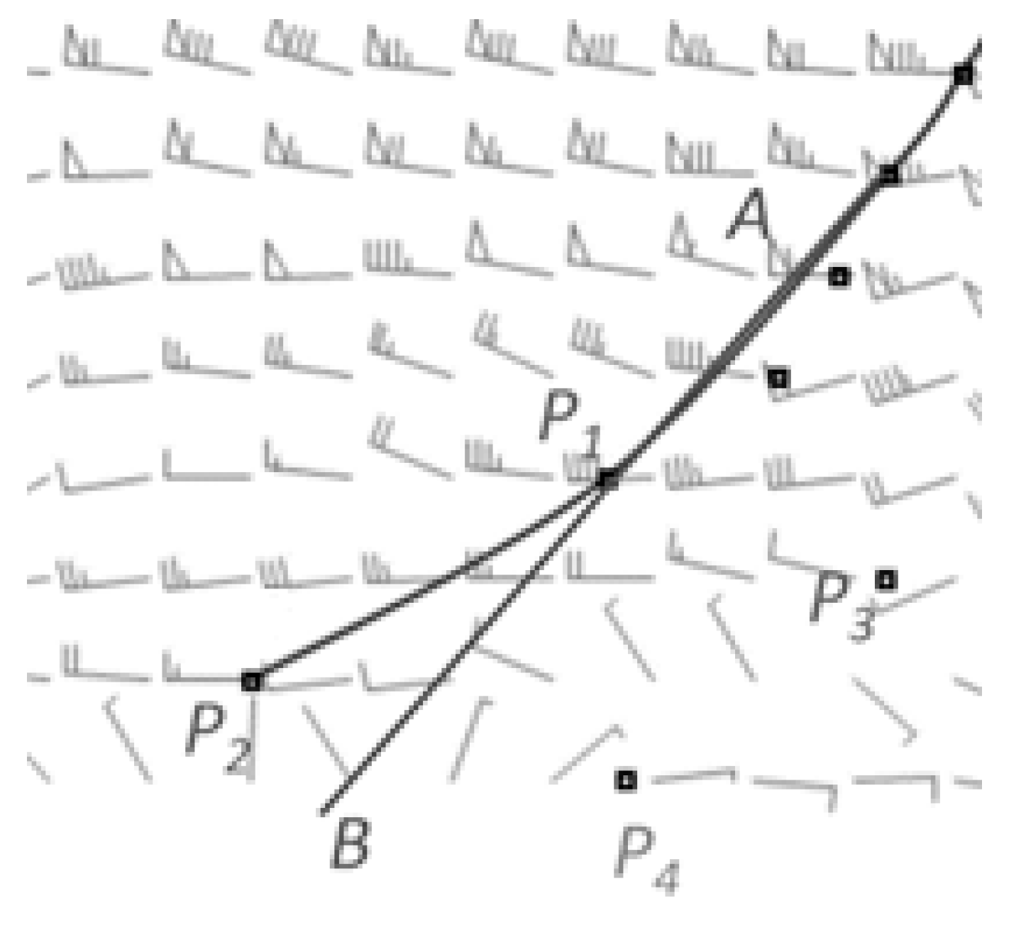
As shown in Figure 1, is the last traced trough point of the current longwave trough, and A is the previous trough point. Two candidate points meet the distance condition, e.g., and , whose distance to is less than the threshold value (the circle whose center is ). The next trough point should be within the range of a certain angle, , whose vertex is and whose angle bisector () is the extension line of , where are auxiliary points to help illustrate the certain angle and its angle bisector. Only point is in this region; thus, should be the next trough point to trace.
Given the above selection restrictions, candidates are further filtered and denoted as . When is an empty set, the tracing is complete. When there is only one point in , it is the next trough point. When there are multiple points in the set, more restrictions should be introduced to select the next trough point traced. Thus, a function is defined to evaluate the points in set according to the distance and angle conditions, and the point with the maximum function value is selected as the next trough point:
where is the distance between the present candidate point and the last traced trough point, is the angle between the line that connects the candidate and the previous trough point and the tracing direction, and is the fixed angle of deflection for the desired tracing direction. and are the weight values for distance and angle, respectively. As shown in Figure 2, point is the current last traced trough point and point A is the previous last traced point; the line is the extension line of the line . For example, for point , the angle , and the distance between and correspond to and , respectively, in
This evaluation function can offer more reasonable trough points. The above restrictions allow us to iteratively trace the longwave trough until all candidate points have been researched. Ultimately, the zigzag trough lines will be replaced by smoother lines.
2.3. Shortwave Trough Analysis
After completely tracing the longwave trough, wind shear, which is represented by angular deflection and vorticity, can be utilized to find the candidate shortwave trough points. Because of the uncrossed rule of trough lines, shortwave candidate points within the longwave trough region should be removed. Then, the remaining candidates can be clustered and fitted to smooth troughs.
2.3.1. Extraction of Shortwave Trough Candidate Points
Because shortwave troughs generally coincide spatially with the cyclonic shear line, we are generally able to locate shortwave troughs based on the significant wind shear region. Specifically, we can select candidate points according to the angular deflection and vorticity of grid points, which are considered crucial factors that affect wind shear [24].
Zonal and meridional angular deflection are calculated according to the wind direction of the grids:
where is the wind direction of the grid, and and represent the angular deflection in the zonal and meridional directions of the wind field. Wind direction around a grid point in the wind shear region generally changes significantly. Therefore, we defined the threshold to select grid points with larger angular deflections as candidate shortwave trough points, as follows:
where is a variable weight and and are the number of rows and columns in the wind grid. A grid point can be regarded as a candidate only if one of its two angular deflection values is greater than the threshold.
Positive/negative signs and the vorticity value indicate the direction and strength of the fluid rotation, and are represented as follows:
where is the partial derivative of the wind speed’s meridional component v and is the partial derivative of the wind speed zonal component . In the Northern Hemisphere, positive vorticity indicates an anticlockwise rotation; thus, we defined the threshold as follows:
where represents the adjustable weight and and are, again, the number of rows and columns of wind grid data. Grids with greater values than the threshold are also selected as candidate points for shortwave trough lines.
2.3.2. Removing and Clustering of Candidate Points
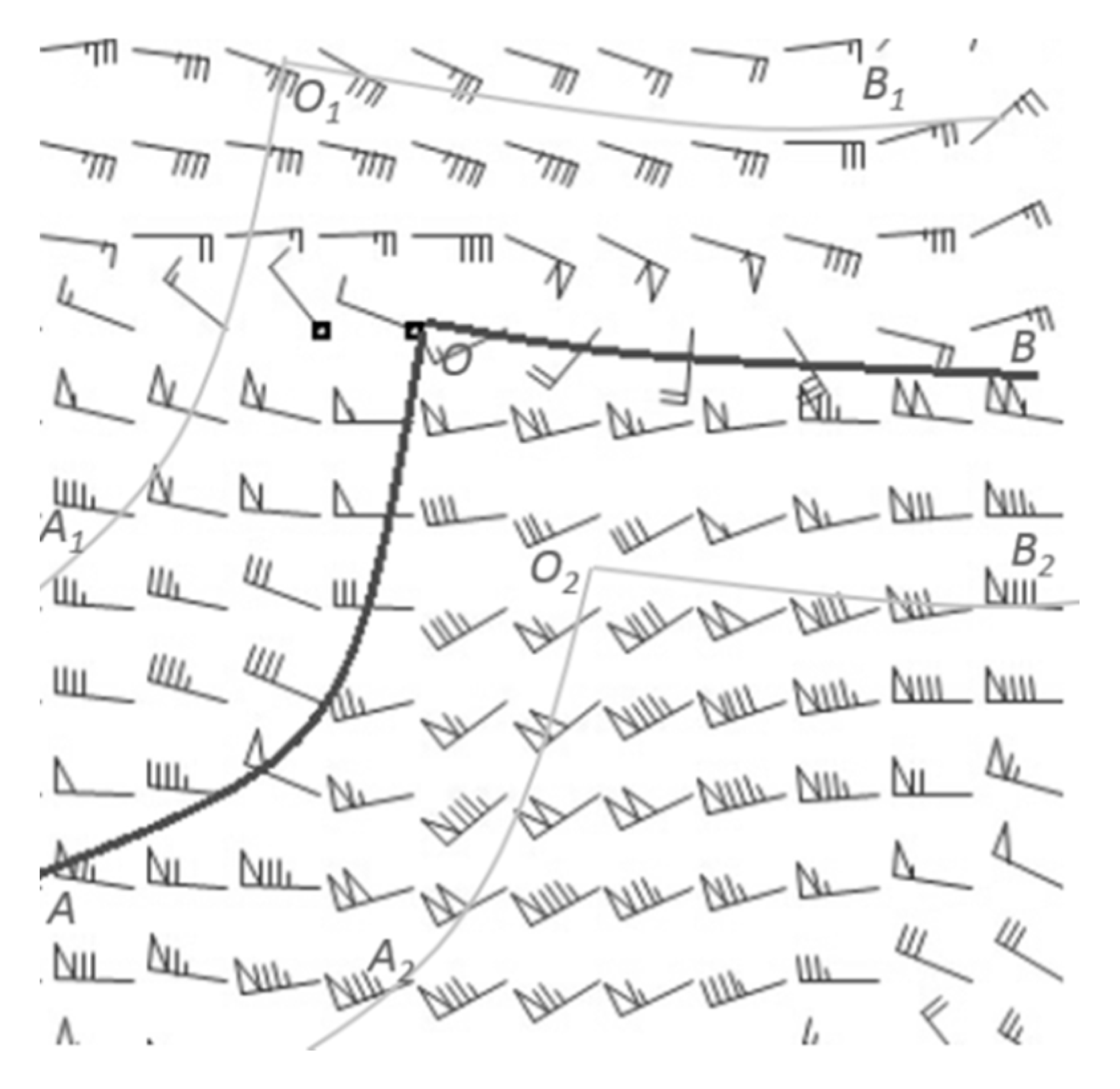
Given that trough lines will never cross each other, candidate shortwave trough points near longwave trough lines should be removed. In our method, we delimit the regions around the longwave trough, the boundaries of which are set parallel to the longwave trough lines. Candidate shortwave trough points are removed if they fall within this region. For example, in Figure 3, and are longwave trough lines, and and are the lines parallel to . Similarly, line and line are parallel to trough line . The distance between the parallel line and the trough line is set according to the spatial resolution of the data. Candidate shortwave trough points within the region defined by and are ruled out to prevent crossed trough lines.
After removing noise candidates, we adopt a minimum-spanning, tree-clustering algorithm [25] to classify and cluster the remaining candidate shortwave trough points. An undirected-weighted, connected graph is constructed to represent the subtree, in which the geometrical distance between trough points is used to define the weight edges for similar trough points. Finally, every subtree can be a point set for one shortwave trough line; therefore, the quartic polynomial [26] is used for curve fitting to favor the smooth shortwave trough line extraction from the point sets.
3. Results and Discussion
We implemented this approach on a personal computer and used wind field data from the National Centers for Environmental Prediction (NCEP) to test it. Section 3.2 demonstrates this approach, and Section 3.3 compares the automatic identification results in this paper to subjective analysis results, using recall ratio and precision ratio data to examine the accuracy and reliability of the method.
3.1. Parameters and Data
The approach was carried out on a PC with an Intel Core i7-3770 CPU, 3.40 GHz, 8 GB of RAM and a 64-bit Windows 7 operating system. In terms of the method’s parameters, considering that the troughs are generally without evident direction change, we set the desired tracing direction as a small angle. The angles from 3° to 10° were tested; when the tracing direction was set at a larger angle, such as 8° or 9°, the trough lines were more zigzaged, and if the angle was relatively small, such as 3° or 4°, there was not enough trough points to trace longwave trough lines. Thus, the fixed angle was set at 5°. In addition, the set of WeightA and WeightB were relatively simple, because the angle condition is often more important than the distance condition in tracing longwave trough lines. The weight values for distance () and angle () were set to 0.6 and 0.8, respectively. Lastly, during the shortwave trough line tracing process, the variable weights of angular deflection () and vorticity () were found to work best at an interval of 2–3. If the β and γ were larger than 3, fewer candidate shortwave trough points would be extracted, which might not obtain reasonable shortwave trough lines; if the β and γ were smaller than 2, it would add lots of noise point to influence the curve fitting of candidate trough points; thus, we tried to use and .
To examine our approach, six-hour re-analysis wind field grid data from NCEP were employed. The data included zonal and meridional wind speed components corresponding to latitude and longitude, and the spatial resolution of the data was 2.5° × 2.5°. We focused on the 500 hPa geopotential height for two reasons. First, the change and movement of air at this height is relatively steady, and the periodic change in the wind field is explicit. Second, most weather processes leave an imprint on the 500 hPa isobaric surface, which can be used to predict future weather changes more accurately. The region we chose for this experiment was 0°–60° N and 60°–180° E, which is widely used for synoptic chart analysis in East and South Asia.
3.2. Case Study
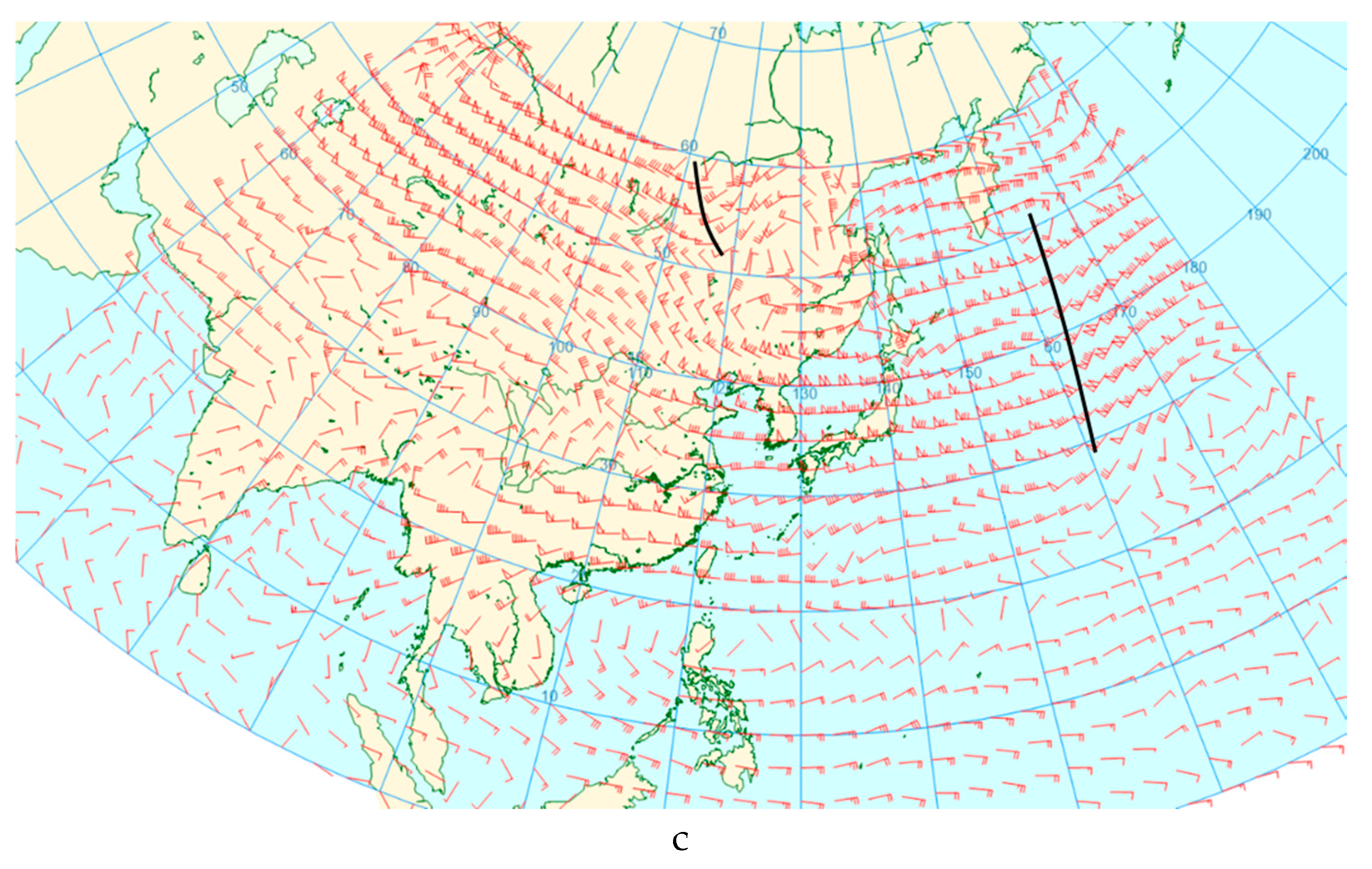
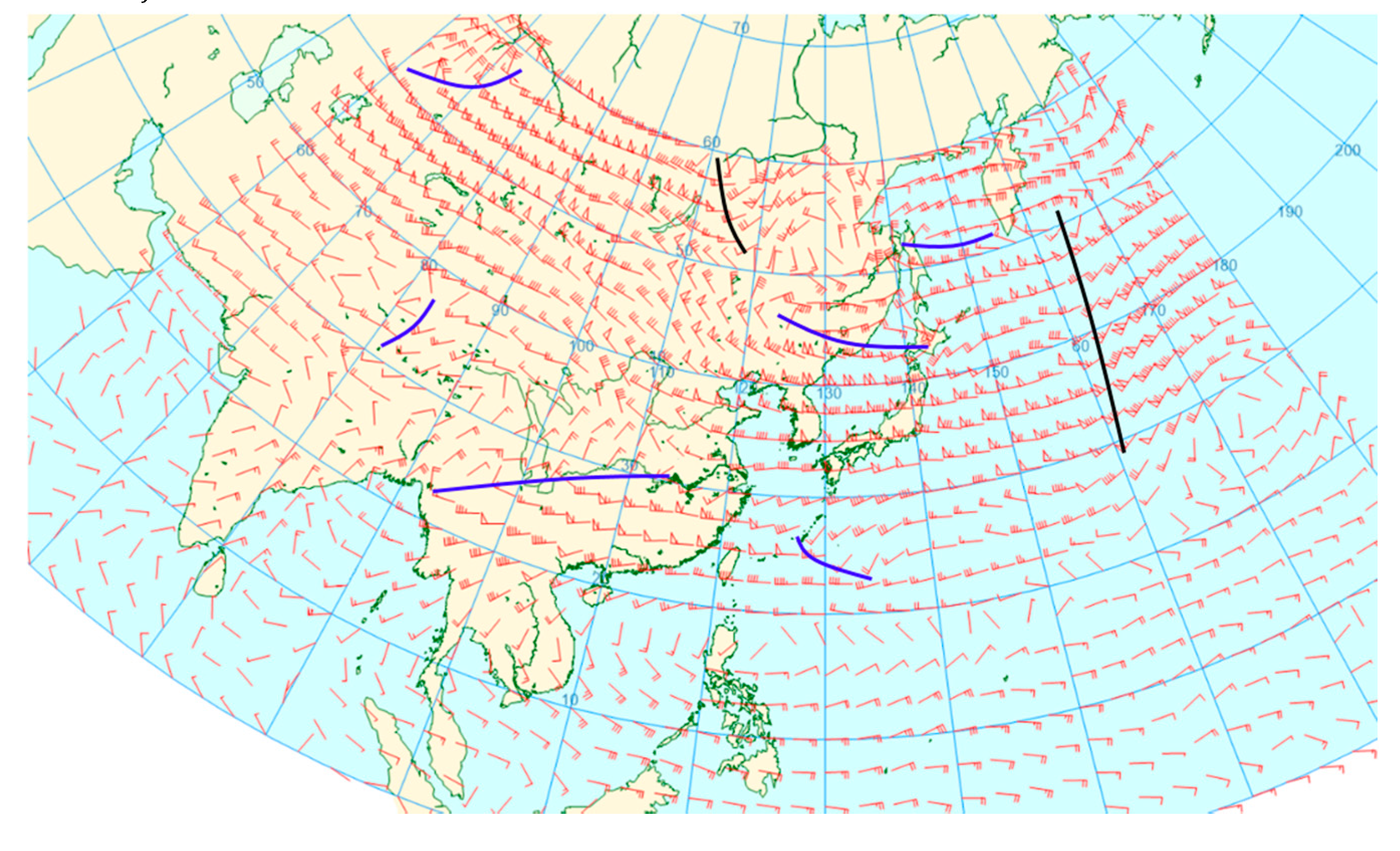
We used wind field data from 30 April 2009 at 1600 UTC to test the validity of the proposed method. The automatic identification results of each step in tracing longwave trough lines (including the extraction of cyclonic centers and candidate longwave trough points) are shown in Figure 4. In Figure 4a, dark spots represent the location of points with local minimum wind speed; the cyclonic centers are extracted from these points using the method proposed in Section 2.2.1. All cyclonic centers were found precisely and were used as the starting points of trough lines. In Figure 4b, the candidate points for longwave trough lines were extracted according to the wind direction of the grid points, as described in Section 2.2.2. The final result of the longwave trough lines analysis is illustrated on a geographic background in Figure 4c, with Lambert projection. Because the tracing direction is constrained to a given scope, few evident bending points can be seen in the trough lines. The evaluated function offers more reasonable trough points, which aids in the acquisition of accurate tracing results.
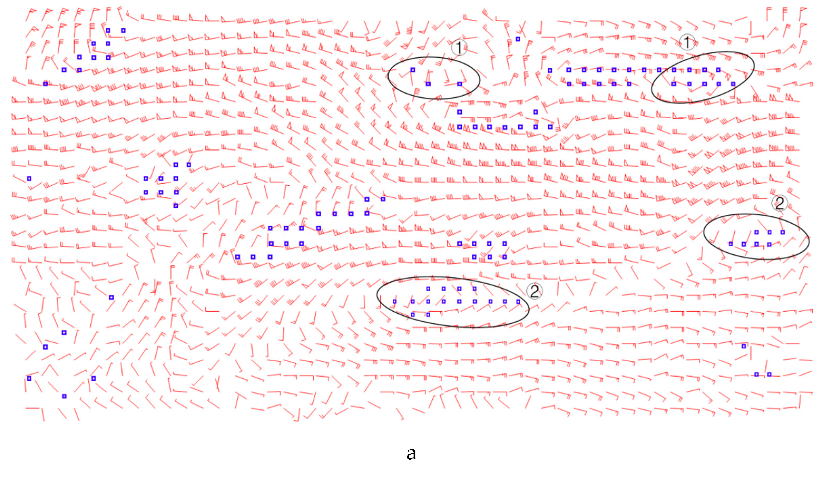
The experimental results from each step of the automatic shortwave trough line identification (including the extraction of candidate shortwave trough points, trough point clustering, and curve fitting) are shown in Figure 5. Figure 5a shows the candidate shortwave trough points that were extracted based on angular deflection and vorticity factors, with those candidates in the longwave trough regions (which are marked with symbol ①) removed, as described in Section 2.3.2. A minimum spanning tree clustering algorithm was applied to obtain some of the shortwave trough point sets. Because trough lines generally appear near low-pressure areas, the candidates around anticyclonic (high-pressure) centers were removed even if the wind shear there was significant, which are marked with symbol ②. Figure 5b shows two examples of the curve fitting for shortwave trough points. In these examples, the quartic polynomial was used to achieve smooth shortwave trough lines from candidate shortwave trough point sets. The final shortwave trough lines produced by the automatic analysis are displayed on a geographic background map in Figure 5c.
The identification result, combined with both longwave and shortwave trough lines, is shown in Figure 6. Compared to the manual analysis performed by forecasters, our method produces results much closer to the subjective result.
Furthermore, 70 groups of wind field data at 500 hPa from 2009 to 2010 were analyzed using our method. Examples of the experimental results from this analysis are shown in Figure 7.
3.3. Comparison and Evaluation
Several experiments were completed to compare our method to the subjective analysis of trough lines. To do so, two professional weather forecasters were invited to help conduct a manual analysis of trough lines using the same wind field data sets, which were taken as ground truth. The objective analysis results from our method were overlaid onto the subjective trough lines derived from the same wind field. We then delineated a rectangular region around each subjective trough line and visually identified whether a matching objective trough line was located within the rectangle of the subjective trough line. We then quantitatively assessed the matching pairs by adopting a quantification judgement method from previous research [27]. The consistency degree was used to measure the location consistency and scope consistency between subjective and objective trough lines. The consistency degree is represented as follows:
Within the rectangular region of a matching pair, is the number of grid points in the objective trough line, is the number of grid points in the subjective trough line, and represents the number of grid points in both trough lines. Particularly, if the subjective trough line crossed between two grid points and at least one of the two points is in the objective trough line, we assumed a coincident point was present, which was then added to . The consistency degree range was set from 0 to 100; a larger degree corresponded to greater similarity between the two trough lines.
The consistency degrees for all matching pairs from wind field data were computed using the aforementioned quantification judgement method, and the partial results (a total of 140 samples, including 70 matching pairs of shortwave trough lines and 70 matching pairs of longwave trough lines, which were selected randomly from all matching pairs) are shown in Figure 8. Figure 8a indicates that most of the matching pairs’ consistency degrees exceeded 60, which means the objective analysis of the location and length of the trough lines is generally consistent with the subjective result. In addition, given the more obvious trends and greater lengths of longwave trough lines, they are identified more exactly than shortwave trough lines, as illustrated in Figure 8b. The orange dotted line in Figure 8b is the polynomial fitting curve about the statistical result of longwave matching pairs’ consistency degree, where the blue represents the polynomial fitting curve of shortwave matching pairs’ consistency degree. It can be seen that the average consistency degree of the major matching pairs of longwave trough lines is approximately 85, while that of shortwave trough lines is approximately 80. The result indicates that the objective identification of longwave trough lines is more exact than longwave trough lines.
According to the advice of the forecasters, if the consistency degree was greater than 60, the trough line identification for a matching pair was viewed as a success. Evaluation criteria, including the recall ratio and precision ratio, were then proposed to examine the accuracy and reliability of our identification method:
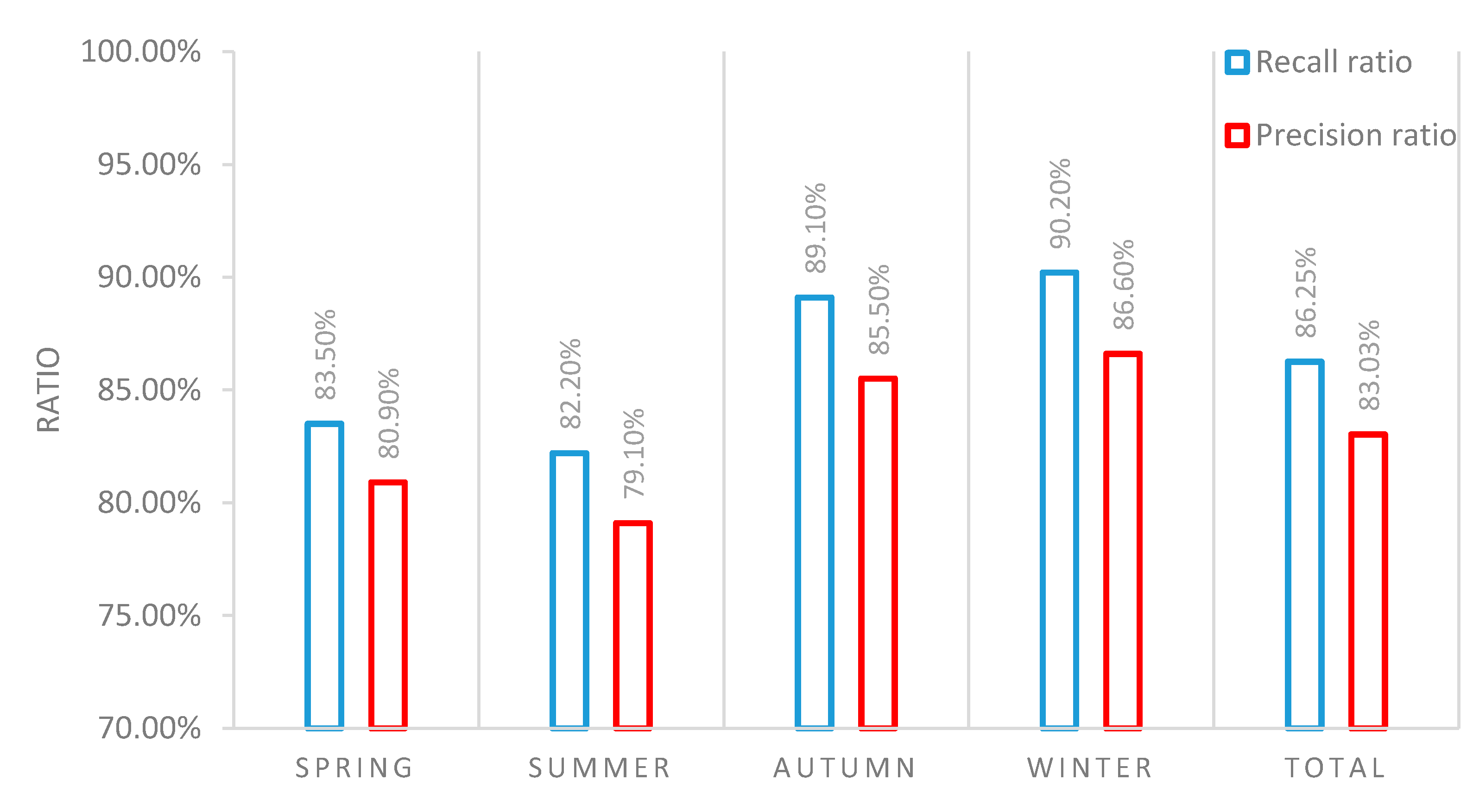
where is the number of successful matching pairs, is the number of subjective trough lines, and is the number of objective trough lines. All trough lines were assessed and the results shown in Figure 9. Based on this analysis, we determined that a more accurate and effective trough line identification process was possible during the fall and winter than during the spring and summer. This may be because the synoptic system is comparatively steady during fall and winter, with evident trends in major troughs; that is, most troughs are longwave troughs, which may be easier to analyze. Nevertheless, the total recall ratio and precision ratio reached 86.25% and 83.03%, respectively, which may meet the practical demands of weather forecasters.
4. Conclusions
In this paper, an objective method for identifying trough lines using wind field data was proposed. Longwave and shortwave trough lines were analyzed in different ways. To analyze longwave trough lines, cyclonic centers were first located and candidate trough points were filtered according to wind direction. Candidate longwave trough points were traced starting from the cyclonic centers (based on distance and angle conditions). Next, shortwave trough candidate points were identified according to the angular deflection and vorticity of grid points, which were then clustered and fitted to a curve to define the shortwave trough lines. Compared to other methods (based on pressure field data), this approach conforms better to the experience and rules of the manual identification of trough lines. Moreover, from a global perspective, the wind direction has more distinct distribution than isolines extracted from pressure field data, which indicates that the method can be used more widely. The experimental results show that longwave trough lines can be more accurately determined than shortwave trough lines relative to manual analysis, because they have more obvious trends and greater lengths. Furthermore, by classifying the recall ratio and precision ratio of the identification results by season, we determined that trough line identification was more accurate and effective during the fall and winter than during the spring and summer. The reason is that synoptic systems during the fall and winter are steadier than those during the spring and summer, potentially resulting in more longwave trough lines; therefore, the analysis is comparatively easy and exact. In general, the method proposed here allows for the objective identification of trough lines and can cater to the practical demands of weather forecasting work.
However, the method might be less robust in areas with irregular wind fields, which may lead to the missed identification of trough lines, and more effort will be made in the future to improve the method. In addition, self-adaptive parameters, according to the different data resolution and wind field features, will be the focus of our future study to achieve better identification results.
Acknowledgments
We thank the editor and reviewers for their careful review and insightful comments. This paper was sponsored by the National Natural Science Foundation of China (No. 41305138 and No. 61473310).
Author Contributions
The work presented here was a collaboration between all authors. Qian Li outlined the method used. Yan Huang and Xi Dai performed the experiments and wrote the manuscript. Yin Fan and Qian Li revised the manuscript
Conflicts of Interest
The authors declare no conflicts of interest.
References
- Henry, R.K.; Welles, E.; Hopkins, T. AWIPS II Overview and Status. Proceedings of 25th Conference on Interactive Information and Processing Systems for Meteorology, Oceanography, and Hydrology, Phoenix, AZ, USA, 15 January 2009. [Google Scholar]
- Yufeng, T.; Qiu, K.; Zhao, X.; Zhang, L. Meteorological Graph Web Displaying Based on the MICAPS System. Meteorol. Environ. Sci. 2008, 4, 018. [Google Scholar]
- Huang, X.; Zhao, F. Relation-based aggregation: finding objects in large spatial datasets. Intell. Data Anal. 2000, 4, 129–147. [Google Scholar]
- Huang, X. Relsa: Automatic analysis of spatial data sets using visual reasoning techniques with an application to weather data analysis. Ph.D. Thesis, The Ohio State University, Columbus, OH, USA, 2000. [Google Scholar]
- Wong, K.Y.; Yip, C.L.; Li, P.W. Automatic identification of weather systems from numerical weather prediction data using genetic algorithm. Expert Syst. Appl. 2008, 35, 542–555. [Google Scholar] [CrossRef]
- Li, Y.; Musilek, P.; Lozowski, E. Identification of atmospheric pressure troughs using image processing techniques. Proceedings of 2013 IFSA World Congress and NAFIPS Meeting, Edmonton, Canada, 24 June 2013; IEEE: New York, NY, USA, 2013; pp. 722–726. [Google Scholar]
- Jann, A. Use of a simple pattern recognition approach for the detection of ridge lines and stripes. Meteorol. Appl. 2002, 9, 357–365. [Google Scholar] [CrossRef]
- Hope, P.; Keay, K.; Pook, M.; Catto, J.; Simmonds, I. A comparison of automated methods of front recognition for climate studies: A case study in southwest Western Australia. Mon. Weather Rev. 2014, 142, 343–363. [Google Scholar] [CrossRef]
- Hewson, T.D. Objective fronts. Meteorol. Appl. 2000, 5, 37–65. [Google Scholar] [CrossRef]
- Hewson, T.D. Tracking fronts and extra-tropical cyclones. ECMWF Newsl. 2009, 121, 9–19. [Google Scholar]
- Jenkner, J.; Sprenger, M.; Schwenk, I.; Schwierz, C.; Dierer, S.; Leuenberger, D. Detection and climatology of fronts in a high-resolution model reanalysis over the Alps. Meteorol. Appl. 2010, 17, 1–18. [Google Scholar] [CrossRef]
- Berry, G.; Reeder, M.J.; Jakob, C. A global climatology of atmospheric fronts. Geophys. Res. Lett. 2011, 38, L04809. [Google Scholar] [CrossRef]
- Ohtake, Y.; Belyaev, A.; Seidel, H.P. Ridge-valley lines on meshes via implicit surface fitting. ACM Trans. Gr. 2004, 23, 609–612. [Google Scholar] [CrossRef]
- Pang, X.F. An Algorithm for Extracting and Enhancing Valley-ridge Features from Point Sets. Acta Autom. Sin. 2010, 36, 1073–1083. [Google Scholar] [CrossRef]
- López, A.M.; Lumbreras, F.; Serrat, J.; Villanueva, J.J. Evaluation of methods for ridge and valley detection. IEEE Trans. Pattern Anal. Mach. Intell. 1999, 21, 327–335. [Google Scholar] [CrossRef]
- Gauch, J.M.; Pizer, S.M. Multiresolution analysis of ridges and valleys in grey-scale images. IEEE Trans. Pattern Anal. Mach. Intell. 1993, 15, 635–646. [Google Scholar] [CrossRef]
- Schultz, D.M. A Review of Cold Fronts with Prefrontal Troughs and Wind Shifts. Mon. Weather Rev. 2005, 133, 2449–2472. [Google Scholar] [CrossRef]
- Wang, Z.L. The influence of the westerly belt long-wave trough over Asia on the western pacific typhoon tracks. Chin. J. Atmos. Sci. 1981, 2, 008. [Google Scholar]
- Tuttle, J.D.; Davis, C.A. Modulation of the Diurnal Cycle of Warm-Season Precipitation by Short-Wave Troughs. J. Atmos. Sci. 2013, 70, 1710–1726. [Google Scholar] [CrossRef]
- Zong, H.; Wu, L. Synoptic-Scale Influences on Tropical Cyclone Formation within the Western North Pacific Monsoon Trough. Mon. Weather Rev. 2015, 143, 3421–3433. [Google Scholar] [CrossRef]
- Helman, J.L.; Hesselink, L. Visualizing Vector Field Topology in Fluid Flows. IEEE Comput. Gr. Appl. 1991, 11, 36–46. [Google Scholar] [CrossRef]
- Helman, J.; Hesselink, L. Representation and display of vector field topology in fluid flow data sets. IEEE Comput. 1989, 22, 27–36. [Google Scholar] [CrossRef]
- Haimes, R.; Kenwright, D. On the velocity gradient tensor and fluid feature extraction. AIAA Pap. 1999, 99, 1–10. [Google Scholar]
- Nolan, D.S.; McGauley, M.G. Tropical cyclogenesis in wind shear: Climatological relationships and physical processes. Cyclone. Format. Triggers Control 2012, 1–36. [Google Scholar] [CrossRef]
- Huang, G.; Dong, S.; Ren, J. A Minimum Spanning Tree Clustering Algorithm Based on Density. Adv. Inf. Sci. Serv. Sci. 2013, 5, 44. [Google Scholar]
- Yan, Z.; Li, D. A Polynomial Fitting Method for Pile's Strain Curves. Urb. Geotech. Investig. Surv. 2012, 1, 173–176. [Google Scholar]
- Gong, Y.; Li, J. The quantified verification method of synoptic meteorology and the application to AREM. Sci. Meteorol. Sin. 2010, 30, 763–772. (In Chinese) [Google Scholar]
Figure 1.
The constraint conditions for longwave trough line seeking.
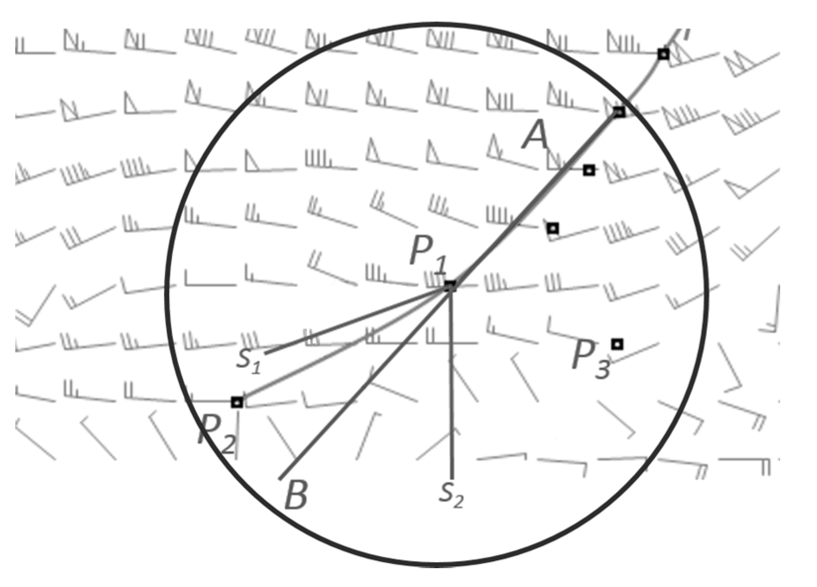
Figure 2.
Selection of the next trough point.

Figure 3.
The areas occupied by the longwave trough line.

Figure 4.
Results from each step of the objective longwave trough lines identification using wind field data from 1600 UTC on 30 April 2009: (a) extraction of cyclonic centers marked by “▲”; (b) extraction of the candidate longwave trough points marked with blue spots; and (c) identification of the longwave trough line (marked with black solid lines).
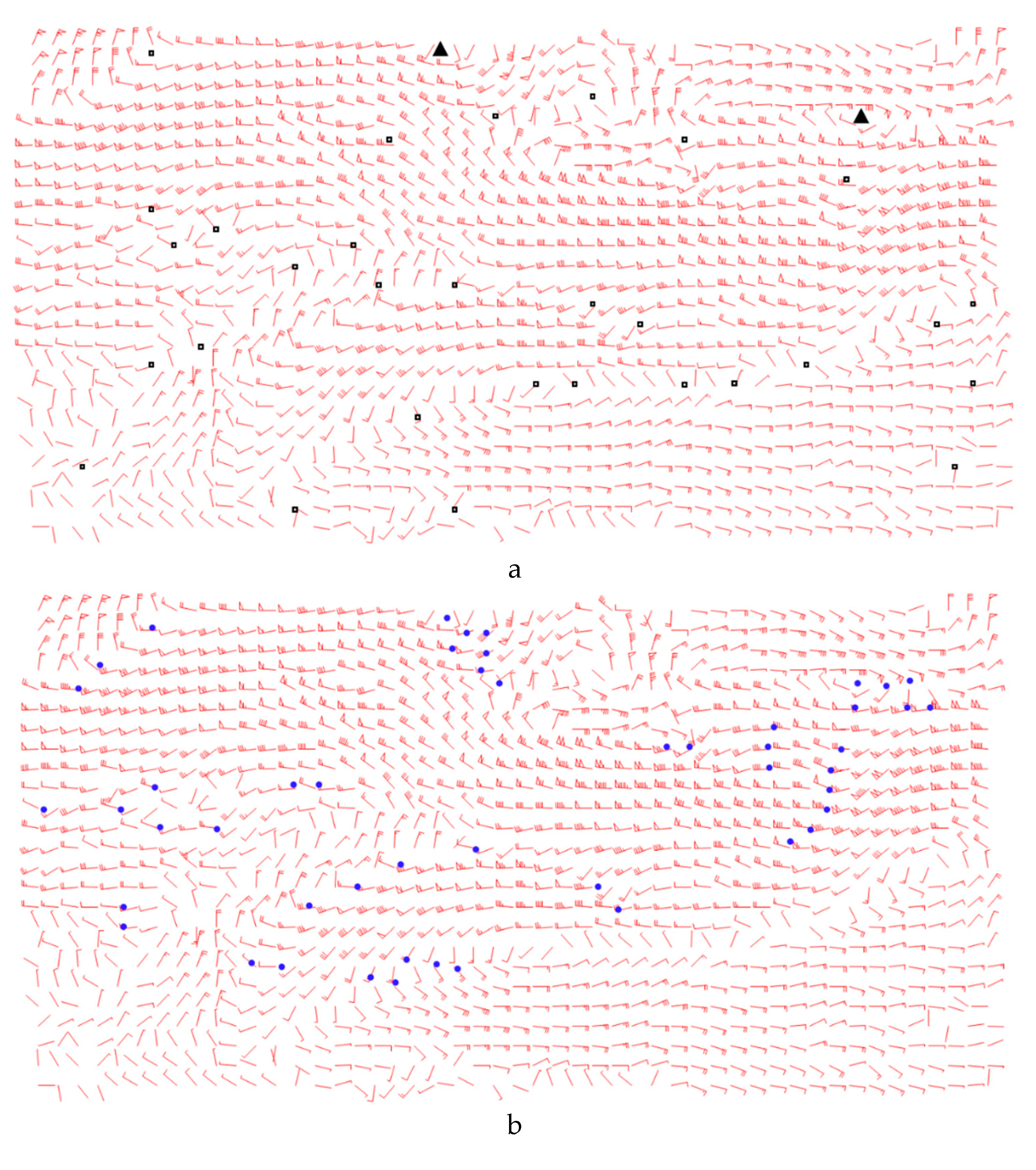

Figure 5.
Result from each step of the objective shortwave trough line identification using wind field data from 1600 UTC on 30 April 2009: (a) extraction of the candidate shortwave trough points, marked with blue spots. The points in the long-wave trough region are marked with ① and in the area of anticyclonic center are marked with ②; (b) curve fitting of the shortwave trough points; (c) identification of the shortwave trough lines (marked with blue solid lines).

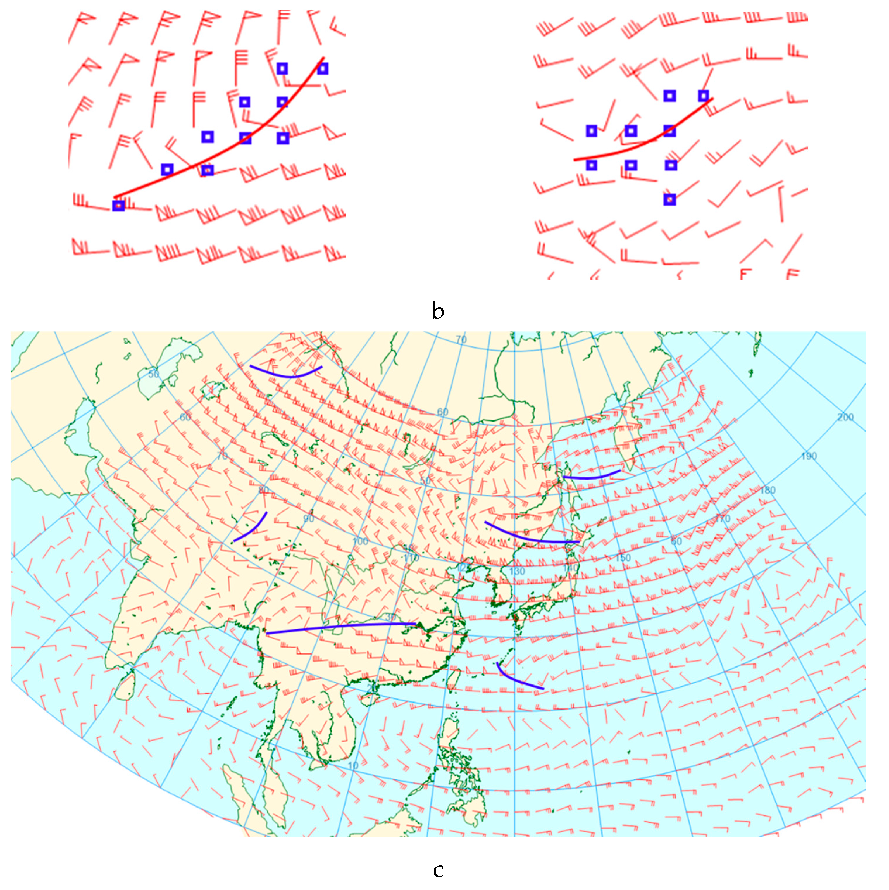
Figure 6.
Objective results from the trough line analysis using data from 1600 UTC on 30 April 2009. The black and blue solid lines represent the longwave and shortwave trough lines, respectively.
Figure 6.
Objective results from the trough line analysis using data from 1600 UTC on 30 April 2009. The black and blue solid lines represent the longwave and shortwave trough lines, respectively.

Figure 7.
(a–d) Objective analysis results of trough line data from 1600 UTC on 30 Sep 2009, 25 Apr 2010, 6 Jun 2010, and 8 Nov 2010. Examples were selected randomly from 70 groups of experimental results. The black solid lines represent longwave trough lines and the blue solid lines are shortwave trough lines.
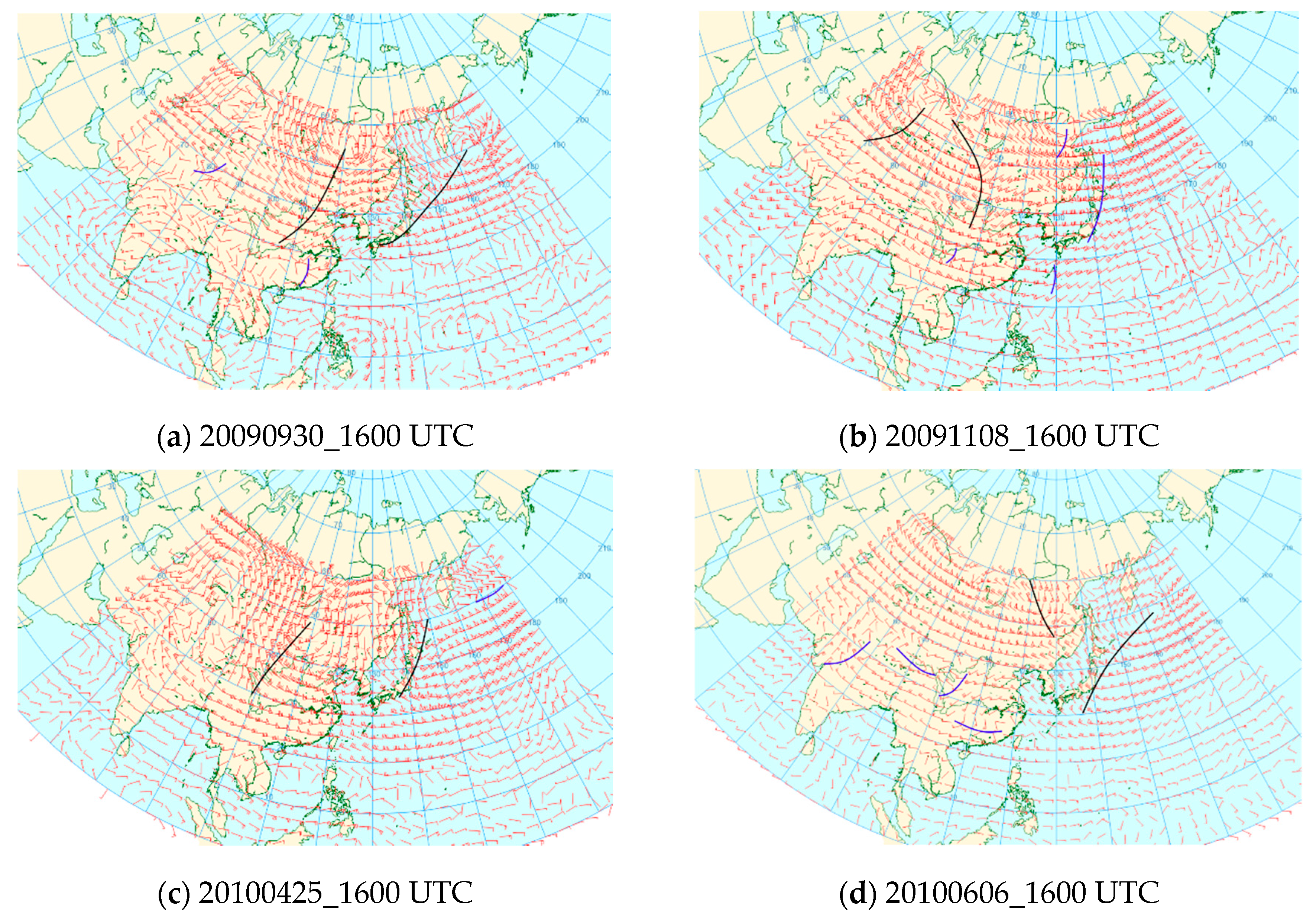
Figure 8.
Results of comparison experiments (a) and the statistical results (b), where the blue and orange dotted lines represent the polynomial fitting of two types of matching pairs, respectively.
Figure 8.
Results of comparison experiments (a) and the statistical results (b), where the blue and orange dotted lines represent the polynomial fitting of two types of matching pairs, respectively.
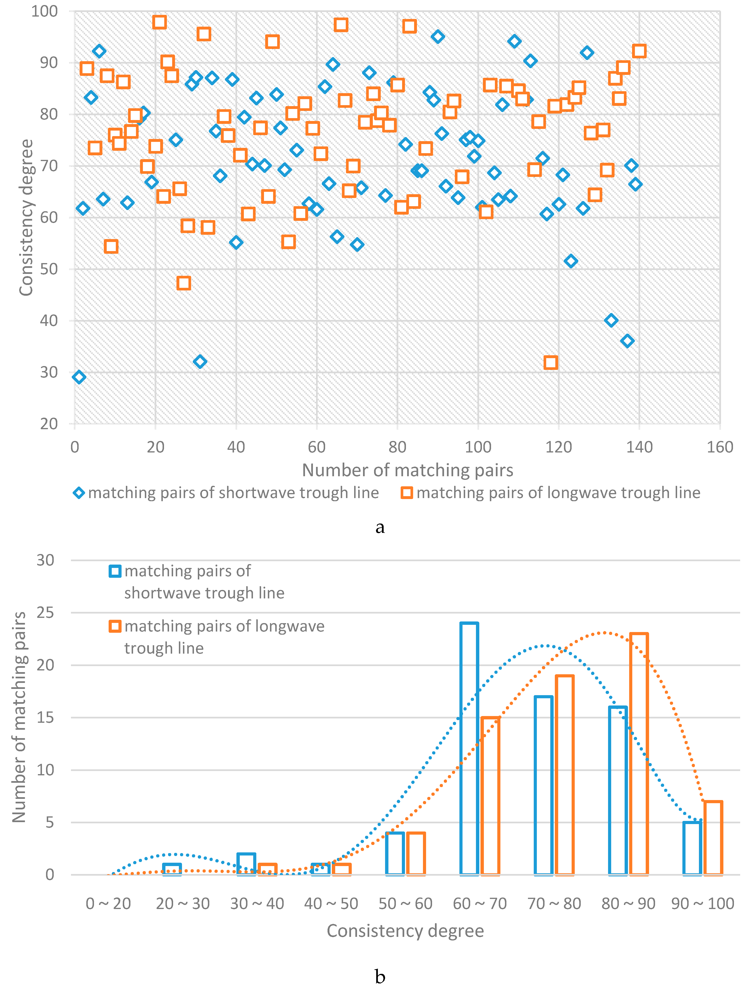
Figure 9.
Recall ratio and precision ratio of the trough line analysis, classified according to season.
Figure 9.
Recall ratio and precision ratio of the trough line analysis, classified according to season.


Table 1.
The corresponding relationship between eigenvalue and topological structure.
| Eigenvalue | Topological Structure |
|---|---|
| Repelling Focus | |
| Saddle Point | |
| Repelling Node | |
| Attracting Focus | |
| Center | |
| Attracting Node |
© 2017 by the authors. Licensee MDPI, Basel, Switzerland. This article is an open access article distributed under the terms and conditions of the Creative Commons Attribution (CC BY) license (http://creativecommons.org/licenses/by/4.0/).
Share and Cite
MDPI and ACS Style
Huang, Y.; Li, Q.; Fan, Y.; Dai, X. Objective Identification of Trough Lines Using Gridded Wind Field Data. Atmosphere 2017, 8, 121. https://doi.org/10.3390/atmos8070121
AMA Style
Huang Y, Li Q, Fan Y, Dai X. Objective Identification of Trough Lines Using Gridded Wind Field Data. Atmosphere. 2017; 8(7):121. https://doi.org/10.3390/atmos8070121
Chicago/Turabian StyleHuang, Yan, Qian Li, Yin Fan, and Xi Dai. 2017. "Objective Identification of Trough Lines Using Gridded Wind Field Data" Atmosphere 8, no. 7: 121. https://doi.org/10.3390/atmos8070121
Note that from the first issue of 2016, this journal uses article numbers instead of page numbers. See further details here.