Observed and Model-Derived Ozone Production Efficiency over Urban and Rural New York State
by
 ,
,
Matthew Ninneman
1,* ,
,
Sarah Lu
1,
Pius Lee
2, 
Jeffery McQueen
3,
Jianping Huang
3, 
Kenneth Demerjian
1 and
James Schwab
1 1
Atmospheric Sciences Research Center, University at Albany, State University of New York, Albany, NY 12203, USA
2
NOAA Air Resources Laboratory, 5830 University Research Court, College Park, MD 20740, USA
3
NOAA National Weather Service, 5830 University Research Court, College Park, MD 20740, USA
*
Author to whom correspondence should be addressed.
Atmosphere 2017, 8(7), 126; https://doi.org/10.3390/atmos8070126
Submission received: 23 May 2017
/
Revised: 28 June 2017
/
Accepted: 15 July 2017
/
Published: 18 July 2017
(This article belongs to the Special Issue Tropospheric Ozone and Its Precursors)
Abstract
:This study examined the model-derived and observed ozone production efficiency (OPE = ∆Ox/∆NOz) in one rural location, Pinnacle State Park (PSP) in Addison, New York (NY), and one urban location, Queens College (QC) in Flushing, NY, in New York State (NYS) during photo-chemically productive hours (11 a.m.–4 p.m. Eastern Standard Time (EST)) in summer 2016. Measurement data and model predictions from National Oceanic and Atmospheric Administration National Air Quality Forecast Capability (NOAA NAQFC)—Community Multiscale Air Quality (CMAQ) model versions 4.6 (v4.6) and 5.0.2 (v5.0.2) were used to assess the OPE at both sites. CMAQ-predicted and observed OPEs were often in poor agreement at PSP and in reasonable agreement at QC, with model-predicted and observed OPEs, ranging from approximately 5–11 and 10–13, respectively, at PSP; and 4–7 and 6–8, respectively, at QC. The observed relationship between OPE and oxides of nitrogen (NOx) was studied at PSP to examine where the OPE downturn may have occurred. Summer 2016 observations at PSP did not reveal a distinct OPE downturn, but they did indicate that the OPE at PSP remained high (10 or greater) regardless of the [NOx] level. The observed OPEs at QC were found by using species-specific reactive odd nitrogen (NOy) instruments and an estimated value for nitrogen dioxide (NO2), since observed OPEs determined using non-specific NOx and NOy instruments yielded observed OPE results that (1) varied from approximately 11–25, (2) sometimes had negative [NOz] concentrations, and (3) were inconsistent with CMAQ-predicted OPE. This difference in observed OPEs at QC depending on the suite of instruments used suggests that species-specific NOx and NOy instruments may be needed to obtain reliable urban OPEs.
1. Introduction
Lower tropospheric ozone (O3) production occurs due to a sequence of photochemical reactions involving volatile organic compounds (VOCs) in the presence of oxides of nitrogen (NOx = nitric oxide (NO) + nitrogen dioxide (NO2)) [1]. O3 concentrations ([O3]) are controlled through reducing anthropogenic emissions of VOCs, NOx, or both VOCs and NOx [2]. Consequently, it is important to understand how VOCs and NOx lead to O3 formation [2]. The concept of ozone production efficiency (OPE) helps gain such an understanding. OPE is defined as the number of O3 molecules formed for every molecule of NOx oxidized [3]. The OPE is often an effective metric for scaling regional O3 formation to the amount of emitted NOx [1]. The OPE can be approximated by determining the slope of a graph of odd oxygen concentration ([Ox] = [NO2] + [O3]) versus the concentration of NOx oxidation products [4]. The second quantity is the difference between reactive odd nitrogen (NOy = NOx + nitric acid (HNO3) + peroxyacetyl nitrates (PANs) + alkyl nitrates (ANs) + organic nitrates + …) and NOx, defined as NOz [3]. This method of approximating OPE emphasizes increases in [O3] concentrations resulting from photochemical production by VOC oxidation, and does not include O3 variations caused by NO titration [5]. Therefore, estimating OPE as the slope of a plot of [Ox] concentration versus [NOz] concentration (∆Ox/∆NOz) is better suited for urban environments, where NOx concentrations ([NOx]) are higher and O3 is more susceptible to NO titration [2].
Previous work studied OPE in urban and rural environments during photo-chemically productive hours that corresponded to little cloud cover and minimal precipitation (i.e., high temperatures and sunlit conditions). Only photo-chemically productive hours were examined because that was when photochemical ozone production is more favorable [6]. Overall, this prior OPE work was done from either a modeling, measurement, or both a modeling and measurement perspective. Lei et al. [7] examined the instantaneous OPE during the 13–15 April 2003 air pollution episode in the Mexico City metropolitan area by using the Comprehensive Air Quality Model with extensions (CAMx). Their modeling study concluded that the OPE ranged from 4 to 10 from 12 p.m. to 5 p.m. local time throughout the episode.
Meanwhile, Hirsch et al. [1] studied OPE from an observational standpoint. They did so for Harvard Forest, a rural area in Massachusetts, from 1990 to 1994 during the months of May to October for each year. The authors specified photo-chemically productive hours going from 11 a.m. to 5 p.m. Eastern Standard Time (EST) for each day studied. They approximated the OPE as ∆O3/∆NOz instead of ∆Ox/∆NOz because Harvard Forest was characterized by low [NOx] concentrations, meaning that widespread NO titration was less likely [1]. With this specification, the authors found that the OPE ranged from 4 to 8, and maximum OPE values occurred in either June or July of each year [1]. More recently, McDuffie et al. [8] examined the OPE using July–August 2014 observations from the Boulder Atmospheric Observatory (BAO), a location near an oil and natural gas basin and urban NOx emissions from Denver, Colorado (CO). To estimate OPE, the authors used OPE = ∆Ox/∆NOz, and they performed the calculation during peak O3 production at BAO (12–6 p.m. mountain daylight time (MDT)). Ultimately, these authors [8] found that the OPE at BAO during July–August 2014 was approximately 6, consistent with relationships between O3 and NOy observed in other parts of the U.S. during the summer (e.g., [9]).
Zaveri et al. [10] used aircraft measurements, surface measurements, and a zero-dimensional Lagrangian box model to study the OPE in an urban plume on the afternoon (2–3:30 p.m. central standard time (CST)) of 22 June 1999 during the Southern Oxidant Study (SOS) field campaign in Nashville, Tennessee (TN). Their results showed that the observation-based and the modeled OPE for Nashville on that afternoon was approximately 5 [10]. However, the modeled OPEs differed depending on whether the OPE calculation included both chemical reaction and dry deposition rates of O3 and NOx or chemical reaction rates of O3 and NOx only, with the latter calculation yielding a higher modeled OPE [10]. In recent work, Travis et al. [11] used observations from the Studies of Emissions and Atmospheric Composition, Clouds and Climate Coupling by Regional Surveys (SEAC4RS) aircraft campaign in August and September 2013, along with output from the Goddard Earth Observing System—Chemistry (GEOS-Chem) model, to examine the factors affecting tropospheric O3 in the Southeast U.S. Part of their analysis studied the OPE (∆Ox/∆NOz) for the Southeast U.S. below 1.5 kilometers (km) altitude during daytime hours (9 a.m.–4 p.m. local time) from August–September 2013 [11]. Their analysis found that the OPEs calculated from the SEAC4RS measurements and the GEOS-Chem model output were in good agreement, with OPEs of 17.4 and 16.7, respectively [11]. These higher OPEs suggest that NOx emissions have decreased over the Southeast U.S. [11]. From the previous studies outlined above, there are two key points to make. First, OPE can be defined in multiple ways, and different methods of calculating OPE can lead to different results. Second, rural areas often exhibit a higher OPE than urban areas because [NOx] concentrations in a rural area are commonly smaller, and the OPE is typically greatest where [NOx] concentrations are smallest [3]. These two points will be revisited again in this paper.
This study extends previous work by analyzing the OPE (∆Ox/∆NOz) in one rural location, Pinnacle State Park (PSP) in Addison, New York (NY), and one urban location, Queens College (QC) in Flushing, NY, in New York State (NYS) during summer 2016. The analysis was conducted by using a combination of air quality model predictions and measurement data, both of which were hourly-averaged. Model predictions of NOx, NOy, and O3 were taken from two versions of the Community Multiscale Air Quality (CMAQ) model, CMAQ Version 4.6 (v4.6), and CMAQ Version 5.0.2 (v5.0.2). Both CMAQ model versions were run at the National Oceanic and Atmospheric Administration (NOAA) as part of the National Air Quality Forecasting Capability (NAQFC). Measurement data of NOx, NOy, and O3 from the Atmospheric Sciences Research Center (ASRC) at the University at Albany, State University of New York (SUNY), and the New York State Department of Environmental Conservation (NYS DEC) air quality monitoring site at PSP were used to calculate the observed OPE at PSP. Measurement data of NOx and O3 from the ASRC and the NYS DEC air quality monitoring site at QC were also used to help compute the observed OPE at QC. However, the NOy and NOz measurements at QC came from a different source for reasons that will be discussed later. Namely, the NOy and NOz measurement data needed to fully calculate the OPE at QC came from four instruments developed by Atmospheric Research & Analysis, Inc. (ARA), an organization based in Cary, North Carolina (NC), USA. Several steps were taken to explore the CMAQ-model predicted and observed OPEs at both sites in more detail. The corresponding analysis approach—in addition to the site, instrument, and model platform descriptions—is presented below.
2. Experiments
2.1. Site Descriptions
2.1.1. Rural Site—Pinnacle State Park
The Pinnacle State Park (PSP) site is located in Addison, NY, a village in southwestern NYS. Its coordinates are 42.09° N and 77.21° W, and it is about 504 m (m) above sea level [12]. The area surrounding PSP contains a variety of vegetation, including a golf course to the northwest; forestlands consisting of deciduous and coniferous trees; pastures and fields; and a 50-acre pond to the site’s south [12]. The two nearest population centers to PSP are Addison and Corning. The village of Addison is about 4 km to the northwest of PSP, and it has a population of approximately 1800 people [13]. The city of Corning is about 15 km to the northeast of PSP, and it has a population of approximately 11,000 people [13]. PSP’s location within NYS is depicted in Figure 1.
2.1.2. Urban Site—Queens College
The Queens College (QC) site is located in Flushing, NY, located in the Queens borough of New York City and with a population of approximately 2.5 million people as of 2015 [13]. The population of New York City is around 8.5 million, and its metropolitan statistical area contains just over 20 million people [13]. The site coordinates are 40.74° N and 73.82° W, and it is about 20 m above sea level [14]. The QC site is adjacent to a running track, soccer field, and tennis courts on the Queens College campus. The area surrounding QC is composed of several major roadways, residential areas, and commercial areas. Specifically, the QC site is surrounded by the Long Island Expressway to the north, the Grand Central Parkway to the south, the Clearview Expressway to the east, and the Van Wyck Expressway to the west. QC’s location within NYS is also shown in Figure 1.
2.2. Instrument and Model Platform Descriptions
NOx measurements at PSP and QC were made by Thermo Model 42-Trace Level (42C-TL and 42i-TL) NOx analyzers maintained by ASRC (at PSP) and NYS DEC (at QC). For clarity, these instruments will henceforth be referred to as ASRC NOx or DEC NOx’. The DEC NOx’ analyzer determines [NOx] concentrations using chemiluminescence that measures the light generated by the NO + O3 reaction (in which all NO is titrated by excess O3) [15,16]. The prime notation is used to describe the DEC NOx’ analyzer because conversion of NO2 (and other more oxidized nitrogen species) was accomplished with a heated molybdenum converter. In contrast, the NOx analyzer at PSP used a species-specific photolytic converter to selectively convert NO2 to NO prior to chemiluminescent detection. NOy data was likewise gathered at PSP by a Thermo 42i-Y NOY analyzer, an instrument that measures NOy by using the same chemiluminescence approach as the DEC NOx’ instrument [17]. This instrument will be referred to as ASRC NOy. At QC, NOy and HNO3 data were obtained from an NOy analyzer developed by ARA that used a continuous two-channel denuder difference method to determine [NOy] (henceforth referred to as ARA NOy) and [HNO3] concentrations [18]. A complete description of the ARA NOy analyzer and the continuous two-channel denuder difference approach is provided by Arnold et al. [18]. Peroxyacetyl nitrates (PANs) and alkyl nitrates (ANs) measurements at QC were made by a Thermo 42i-TL NOx analyzer implemented by ARA that used a continuous three-channel thermal-photolytic difference technique to make the measurements [19]. Specifically, the first channel measured NOx; the second channel (a 160 degree Celsius (C) thermo-converter) measured NOx and NO2 produced by PANs; and the third channel (a 380 degree C thermo-converter) measured NOx and NO2 produced by PANs and ANs [19]. A detailed schematic of this analyzer and how it measured PANs and ANs at QC is given by Figure S1 in the Supplement. Moreover, particulate nitrate (pNO3) data was gathered at QC by a Total Particulate Nitrogen (TPN) system that used a continuous three-channel denuder-filter difference approach developed by ARA [20]. A full description of the TPN system and its continuous three-channel denuder-filter difference method is provided by Edgerton et al. [20]. Finally, a Teledyne Model T400 Ultraviolet (UV) Absorption O3 Analyzer measured O3 at PSP and QC by absorbing a 254 nanometer (nm) UV light signal [21]. The amount of the light signal absorbed was proportional to the [O3] concentration [21]. Since these instruments were both owned by the NYS DEC, they will be referred to as DEC O3 for clarity.
Additionally, summer 2016 NOx, NOy, and O3 model predictions came from two model platforms—Community Multiscale Air Quality (CMAQ) model version 4.6 (CMAQ v4.6), the former operational version for the National Oceanic and Atmospheric Administration National Centers for Environmental Prediction’s (NOAA NCEP’s) production suite, and CMAQ v5.0.2, an updated version of CMAQ v4.6 that became operational on 14 June 2017 [22]. Both model versions were run at 12 km resolution, and meteorological predictions (e.g., temperature, wind speed, etc.) from the NCEP North American Mesoscale (NAM) model were used to drive CMAQ. The anthropogenic and biogenic emissions inventories used by CMAQ v4.6 and CMAQ v5.0.2 were based on the 2011 National Emissions Inventory (NEI) and the Biogenic Emissions Inventory System (BEIS) version 3.14, respectively [22]. A complete description of how the 2011 NEI and BEIS version 3.14 were created can be found in U.S. EPA [23] and Pouliot and Pierce [24], respectively. The chemical mechanism used for both model simulations was the Carbon Bond Mechanism Version 5 (CB05) [22]. Non-mobile emissions were left at 2011 NEI levels in both CMAQ model versions [22], but their mobile emissions were scaled, as discussed below. Three differences between CMAQ v4.6 and CMAQ v5.0.2 are important to note. First, CMAQ v4.6 used a mobile source emissions inventory that was scaled based on the 2005–2011 trend derived from the United States Environmental Protection Agency Air Quality System (U.S. EPA AQS) records [22]. In contrast, CMAQ v5.0.2 used a mobile source emissions NOx inventory that was scaled based on the 2011–2014 trend derived from U.S. EPA AQS records and satellite data [22]. Second, dry deposition velocities were calculated offline for CMAQ v4.6 and inline for CMAQ v5.0.2 [25]. Third, biogenic emissions rates were calculated offline for CMAQ v4.6 and inline for CMAQ v5.0.2 [25].
2.3. Analysis Approach
The OPE (∆Ox/∆NOz) for PSP and QC was studied from June–September and August–September 2016, respectively, using (1) NOx, NOy, and O3 model predictions from CMAQ v4.6 and CMAQ v5.0.2, and (2) ASRC NOx, ASRC NOy, and DEC O3 measurements at PSP and DEC NOx’, ARA NOy, HNO3, PANs, ANs, pNO3, and DEC O3 measurements at QC. All CMAQ model predictions were put in Network Common Data Form (NetCDF) files, and the necessary output was extracted from those files by using a Grid Application Development Software (GrADS) script. Quality assurance and quality control of the measurement data was done by ASRC and ARA.
Additionally, the model-predicted [NOz] and [Ox] concentrations at both sites were computed by using Equations (1) and (2):
where CMAQ [NOz] and CMAQ [Ox] represent either CMAQ v4.6 or CMAQ v5.0.2-predicted [NOz] and [Ox] concentrations, respectively. Next, the observed [NOz] and [Ox] concentrations at PSP were determined by Equations (3) and (4):
where the ASRC [NO2] concentration in (4) is taken from the ASRC NOx analyzer. In contrast, a different approach was used to compute the observed [NOz] at QC, as shown by Equation (5):
where ARA [NOz] specifies that the observed [NOz] concentrations at QC were found using available data from ARA. In addition, an estimate for the observed [NO2] concentration was calculated using Equation (6) to help determine the observed [Ox] concentration at QC:
where the DEC [NO] concentration is taken from the DEC NOx’ analyzer. Then, an estimate for the observed [Ox] concentration at QC was found by taking the sum of Equation (6) and DEC [O3] (Equation (7)):
CMAQ [NOz] = CMAQ [NOy] − CMAQ [NOx]
CMAQ [Ox] = CMAQ [NO2] + CMAQ [O3]
[NOz] = ASRC [NOy] − ASRC [NOx]
[Ox] = ASRC [NO2] + DEC [O3]
ARA [NOz] ≈ [HNO3] + [PANs] + [ANs] + [pNO3]
[NO2]estimated = ARA [NOy] − ARA [NOz] − DEC [NO]
[Ox]estimated = [NO2]estimated + DEC [O3]
Observed [NOz] and [Ox] concentrations were calculated differently at QC because it was found that, when the method of calculating observed NOz and Ox for PSP was also applied to QC, widely varying monthly OPEs at QC were observed. This was an issue for multiple reasons, as will be discussed in more detail later. As a result, data primarily from ARA was used to determine the observed OPE at QC. Due to ARA data availability, the observed and model-derived OPEs at QC were assessed from August–September 2016 instead of June–September 2016.
Using CMAQ v4.6 output, CMAQ v5.0.2 output, and observations, the OPE at PSP and QC was analyzed on a monthly basis during photo-chemically productive hours (11 a.m.–4 p.m. EST) during summer 2016 by (1) calculating and plotting the slope and y-intercept of a graph of Ox versus NOz, and (2) calculating the coefficient of determination (R2). All model-predicted and observed standard errors and p-values for the OPE analyses at PSP and QC are given in Table S1 in the Supplement. The OPE plots for this study were generated using robust linear regression with bisquare weights in Matrix Laboratory (MATLAB) version R2012b, where extreme outliers in the data were neglected and mild outliers in the data were down-weighted through the use of a tuning constant [26]. Although defining the OPE as ∆Ox/∆NOz has the advantage of only focusing on photochemical O3 production by VOC oxidation, instead of O3 variations caused by NO titration [5], there are some potential limitations associated with this definition. Namely, if there is considerable dry depositional loss of HNO3, the OPE is biased high due to the reduction in the [NOz] concentration [4,9,27,28]. In addition, not only does the specification of the OPE as ∆Ox/∆NOz exclude the effect of dry deposition, it also does not account for mixing and fresh emissions [10]. As a result, OPE = ∆Ox/∆NOz can be regarded as an upper limit for describing how efficiently O3 can be produced [10].
Moreover, two data filters were applied to ensure that the OPE was studied at times where it could be most enhanced. First, times where model-predicted and observed temperatures were less than 20 degrees Celsius (°C) were neglected. Additionally, times where CMAQ-predicted solar radiation reaching the surface was less than 500 watts per square meter (W m−2) was also neglected. Since solar radiation measurements were not made at QC, the observations at PSP and QC were filtered for solar radiation using hourly global irradiance for the closest one-tenth of a degree latitude and longitude at both locations [29]. The hourly global irradiance data was taken from the Perez Diffuse Radiation Model, and details regarding this model are in Perez et al. [30].
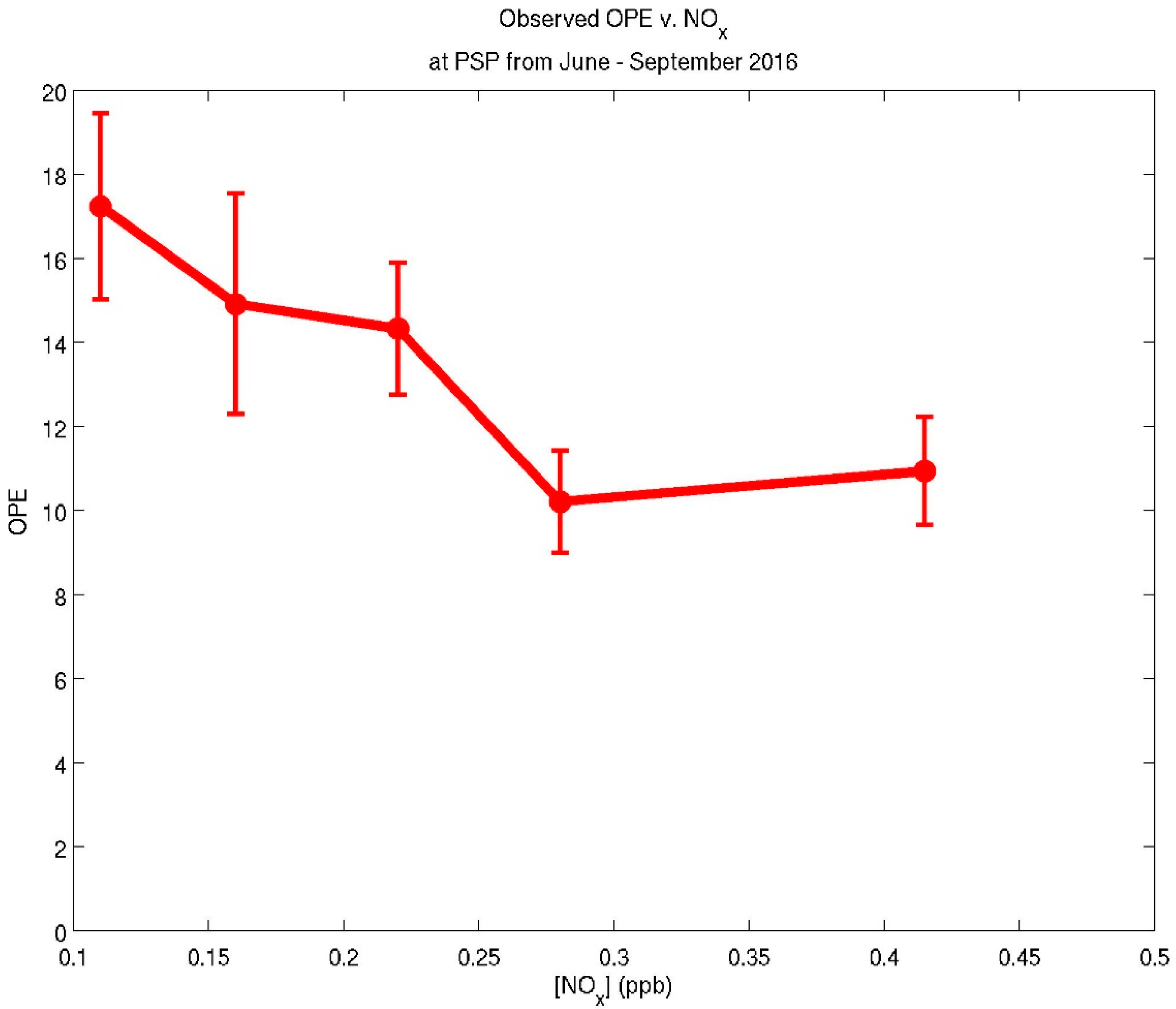
To study the OPE over PSP in greater detail, the observed relationship between OPE and NOx was explored. Since PSP is characterized by lower [NOx] concentrations, it may straddle the NOx regime where values of OPE are rapidly changing. Specifically, there may be a “downturn” where, at a [NOx] concentration on the order of 0.2 parts per billion (ppb) for example, OPE is maximized if [NOx] concentrations are less than 0.2 ppb, and OPE rapidly decreases if [NOx] concentrations are greater than 0.2 ppb [3]. To the best of our knowledge, little work has been done to examine the observed dependence of OPE on [NOx] in a rural, low-NOx environment using the approach described below.
Several steps were taken to complete the OPE versus [NOx] analysis for PSP from June–September 2016. First, observed [NOx] concentrations over the four-month period were divided into five bins, where the sample size was approximately the same in each bin (Table 1). Next, the OPE (∆Ox/∆NOz) was calculated within each bin. Then, the OPE of each bin was plotted as a function of the median [NOx] concentration of each bin (Figure 2). Each point on the plot had corresponding error bars that were plus or minus one standard error of the calculated OPE. The observed standard errors and p-values for the OPE versus [NOx] analysis at PSP are given in Table S2 in the Supplement.
At QC, the observed OPEs were calculated two different ways as noted above, and each type of observed OPE was compared to model predictions. Specifically, the observed monthly OPE results generated for August–September 2016 using (1) the same approach as the one taken at PSP, using in this case NOx and NOy measurements taken from NYS DEC (DEC NOx’ and DEC NOy), and (2) the approach previously described that used ARA data to help calculate the observed OPE, were compared. For the first approach, the DEC NOy instrument at QC is identical to the ASRC NOy instrument at PSP. The only difference is that the DEC NOy instrument at QC is maintained by NYS DEC, and the ASRC NOy instrument at PSP is maintained by ASRC. In sum, a comparison of the results of these two approaches is important because it highlights the potential significance of using species-specific NOx and NOy instruments to better calculate observed OPEs in an urban area.
3. Results
3.1. OPE Analysis Results
Table 2 summarizes the CMAQ v4.6-predicted, CMAQ v5.0.2-predicted, and observed monthly OPEs at PSP from June–September 2016, where the OPE was defined as the slope of the plot of [Ox] versus [NOz], the concentrations of which were determined by Equations (1) and (2) for the model results, and (3) and (4) for the observations. This table indicates that the model-predicted and observed OPEs were often in poor agreement at PSP. Specifically, model-predicted June and September OPEs were about half the observed June and September OPEs. Table 2 also shows the monthly y-intercepts (background [O3] concentrations in ppb), and R2 values at PSP determined by plotting [Ox] concentrations versus [NOz] concentrations for CMAQ v4.6, CMAQ v5.0.2, and the observations. The monthly OPE plots for PSP can be found in Figures S2–S5 in the Supplement. From Table 2, there are three key features to note. First, the observed monthly OPEs of 10.89 (June), 11.38 (July), 11.94 (August), and 13.08 (September) were consistently higher than the model-predicted monthly OPEs. This was partially due to observed [NOx] concentrations being consistently lower than model predictions over the four-month period (Figures S6–S9). Next, even though the predicted and observed July OPEs at PSP were in good agreement, there was a low observed correlation between Ox and NOz (R2 = 0.20). This suggests that the close agreement in model-derived and observed July OPEs may be due to measurement uncertainty rather than improved CMAQ model performance. Moreover, the model-predicted background [O3] concentrations (that is, the y-axis intercepts of the regression lines) noticeably deviated from the observed background [O3] concentrations in July and September. Namely, the models underpredicted background O3 by approximately 6–8 ppb in July and overpredicted background O3 by approximately 7–8 ppb in September. These three features suggest that (1) both CMAQ model versions may be ineffective in predicting the OPE in a rural environment, and (2) observed OPEs of approximately 10 or greater at PSP for this period are consistent with observed OPEs for recent work done in rural areas in the southeastern U.S. [31].
Table 3 shows the CMAQ v4.6-predicted, CMAQ v5.0.2-predicted, and observed monthly OPEs at QC from August–September 2016, where the observed OPE was defined as the slope of the plot of [Ox]estimated versus ARA [NOz], the concentrations of which were calculated by Equations (5) and (7), respectively. This table indicates that the model-predicted and observed OPEs at QC were in good agreement, differing by no more than approximately 2 during the study period. In addition, the August and September observed OPEs of 7.70 and 6.16 are comparable to OPEs observed in other urban areas (e.g., [4,5,10]). The monthly background [O3] concentrations and R2 values at QC found by plotting [Ox] concentrations versus [NOz] concentrations for both CMAQ model versions and the observations are also given in Table 3. These results show that (1) the model-predicted and observed background [O3] concentrations at QC differed by approximately 1–2 ppb in August and 8–10 ppb in September, and (2) model-predicted and observed Ox and NOz were well-correlated, with model-derived and observed R2 values greater than 0.50 for both months. However, it is important to note that the agreement between model-predicted and observed OPE results at the site differed greatly depending on whether (1) the same approach as the one taken at PSP was used, or (2) the approach outlined in Section 2.3 and presented above was used. A comparison of the monthly results of both approaches and the key differences between them is presented in Section 3.3.
3.2. OPE vs. NOx Results: PSP
The observed relationship between OPE and NOx at PSP during summer 2016 is shown in Figure 2. In Figure 2, the observations do not reveal a clear OPE downturn. This is because, when the uncertainty in the OPE calculations for each NOx bin is considered, there may have been little to no change in the OPE as a function of the [NOx] level at PSP during summer 2016. Nevertheless, the relatively constant OPEs at very low [NOx] concentrations (e.g., 0.2 ppb or lower) is qualitatively consistent with previous work presented by Seinfeld and Pandis [3]. Moreover, it is noteworthy that, regardless of the [NOx] level in Figure 2, the OPE remained reasonably high at PSP, with calculated OPEs of 10 or greater for each NOx bin. This may have important implications from a policy perspective, as will be discussed later.
3.3. Comparison of OPE Calculation Approaches: QC
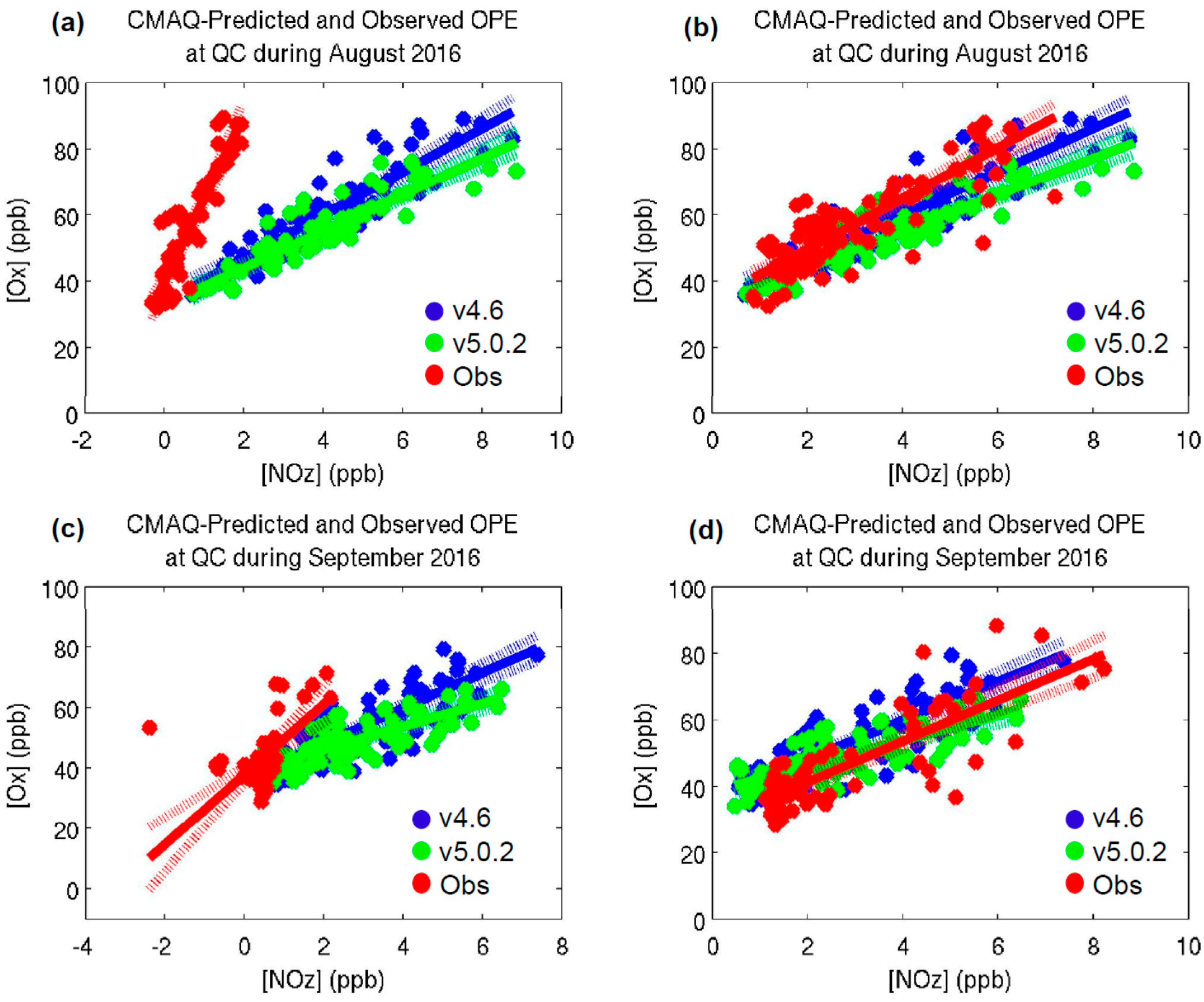
Figure 3a–d and Table 4 compare the model-predicted and observed OPEs at QC during August–September 2016 using (1) DEC NOy and DEC NOx’ (approach 1 or A1), and (2) the approach for QC using ARA data described in Section 2.3 and the results of which were presented in Section 3.1 (approach 2 or A2). As shown by Figure 3a–d and Table 4, model predictions are identical, going from panel (a) to panel (b) and from panel (c) to panel (d), while the observations change dramatically. The results of the OPE analyses for both CMAQ model versions are not relisted in Table 4 since they were already presented in Table 3. From Figure 3a–d and Table 4, the observed OPEs differed greatly depending on the approach used. Specifically, for August 2016, the A1 observed OPE was approximately 3 times greater than the A2 observed OPE. In addition, the A1 observed OPE of 25.11 agreed poorly with the CMAQ v4.6-predicted and CMAQ v5.0.2-predicted OPEs of 6.56 and 5.53, respectively. Conversely, the A2 observed OPE of 7.70 was in good agreement with the CMAQ v4.6-predicted and CMAQ v5.0.2-predicted OPEs of 6.56 and 5.53, respectively. The September 2016 findings told a similar story. Namely, the A1 observed OPE of 11.63 was noticeably greater than the CMAQ v4.6-predicted and CMAQ v5.0.2-predicted OPEs of 5.83 and 3.80, respectively. In contrast, the A2 observed OPE of 6.16 was in good agreement with the CMAQ v4.6-predicted and CMAQ v5.0.2-predicted OPEs of 5.83 and 3.80, respectively. Moreover, Figure 3a,c illustrates that some of the A1 observed [NOz] concentrations were negative, whereas Figure 3b,d shows that all of the A2 observed [NOz] concentrations were positive. This revealed another issue with using A1 to compute observed OPEs at QC because, by definition, [NOz] concentrations should not be negative. Overall, the stronger agreement between the A2 observed and model-derived OPEs, coupled with the more consistent A2 observed OPEs from August to September, provide evidence to suggest that the use of species-specific NOx and NOy instruments are needed to generate observed urban OPE results that (1) do not exhibit potentially unrealistic monthly fluctuations, (2) do not have any negative [NOz] concentrations, and (3) are more comparable to model-derived OPEs. Further discussion on this topic is provided in the next section.
4. Discussion
The lack of consistent agreement between CMAQ-predicted and observed OPE at PSP was undoubtedly due in part to the overprediction in [NOx] concentrations during summer 2016 (Figures S6–S9). According to Figures S6–S9, the use of an updated mobile source emissions NOx inventory in CMAQ v5.0.2 that was scaled based on more recent (2011–2014) air quality trends derived from U.S. EPA AQS records and satellite data [22] appeared to make little difference in CMAQ’s ability to predict [NOx] concentrations at PSP.
To further explore why there was often poor agreement in the model-derived and observed OPEs at PSP, the observed OPEs were determined differently compared to what was presented in Table 2 and Figures S2–S5. Specifically, rather than calculating monthly OPEs by aggregating one month of data (Table 2, Figures S2–S5), where the slope of Ox versus NOz may have been taken over data from heterogeneous meteorological and chemical conditions, daily OPEs were computed at PSP from June–September 2016. These daily OPEs were then averaged to determine new monthly OPEs. Two steps were taken to calculate these new monthly OPEs. First, daily OPEs were calculated for days where at least four out of six photo-chemically productive hours met the temperature and solar radiation filter criteria previously specified. Second, only the daily OPEs that had corresponding R2 values of 0.4 or higher were considered, and these daily OPEs for a given month were averaged to find new monthly OPEs. For completeness, this additional analysis was completed at QC from August–September 2016. A comparison of (1) the monthly OPEs determined by aggregating one month of data, and (2) the new monthly OPEs found by averaging the daily OPEs that met the above filter specifications, is provided in Table S3 in the Supplement for both sites. Example daily OPE plots for 7 August 2016 at PSP and QC are given by Figures S10 and S11, respectively, in the Supplement. Table S3 shows that the monthly OPEs from both approaches generally agree within 1 to 2 of each other. However, a notable exception to this is the July OPEs at PSP, where the observed OPE found by aggregating the July data was 11.38, and the observed OPE found by averaging the daily July OPEs was only 2.05. Two potential factors may have contributed in part to this discrepancy at PSP. The first possible factor is the low correlation (R2 = 0.20) between Ox and NOz when all of the July OPE data is considered (Table 2). The second possible factor is the frequent daily fluctuations in Ox, NOz, or both Ox and NOz during photo-chemically productive periods in July. Such daily fluctuations often led to either large positive or large negative daily July OPEs that were not characteristic of the other three summer months. Overall, both of these factors may have been caused by measurement uncertainty, additional meteorological and chemical processes (e.g., dry deposition of O3 or NOy) that were beyond the scope of this study, or a combination of the two. Nevertheless, the otherwise good agreement between the two approaches suggests that computing observed OPEs over an extended period of time (e.g., a month) is a reliable method, as long as proper data filters are applied to ensure that only more homogeneous conditions characterized by high temperatures and high insolation are considered and R2 values are in the 0.4–0.5 range or higher. As a result, it is hypothesized that the largely poor agreement between model-derived and observed OPEs at PSP is mostly due to poor model performance.
To address the above hypothesis, an important area of future work involves examining the VOC reactivity at PSP using both CMAQ and observations. Analyzing the VOC reactivity is important because, during the O3 formation process, a competition exists between NOx and VOCs for the hydroxyl (OH) radical, the major reactive species involved in O3 formation chemistry [3]. At low [NOx] concentrations such as those observed at PSP, OH preferentially reacts with VOCs to form O3 [3]. Previous work has studied VOC reactivity using a combination of the CMAQ model and surface observations in multiple locations (e.g., [32]), but not for PSP. Consequently, examining the VOC reactivity at PSP will likely help in further understanding the mechanisms behind tropospheric O3 production and the resulting OPE at this site. Thus, such an analysis may help reveal why neither CMAQ model version accurately predicted the OPEs observed at PSP.
Additionally, the observed OPE values of approximately 10 or higher at PSP during summer 2016 are consistent with (1) results from recent studies and (2) the notion that rural areas typically have a greater OPE than urban areas [3]. As previously mentioned, aircraft measurements made by Travis et al. [11] over the Southeast U.S. during August and September 2013 yielded an OPE of 17.4. The consistency between the observed OPE at PSP and the OPE observed over the Southeast U.S. indicates that the OPE has increased in NOx-sensitive areas throughout the eastern U.S. compared to the 1990s, where the OPE in NOx-sensitive areas was typically around 4 to 8 [1]. A likely reason for the recent increase in OPE is the decrease in ambient [NOx] concentrations in the eastern U.S. [11,31].
Although the observed OPE versus NOx relationship at PSP did not reveal a distinct OPE downturn, Figure 2 shows that the OPE at PSP was 10 or greater, even at [NOx] concentrations on the order of 0.4 ppb. This feature may present a challenge to air quality regulators for two main reasons. First, it suggests that, regardless of the [NOx] level, OPEs remain relatively high. In addition, the O3 production rate scales with [NOx], while the OPE is inversely related (i.e., higher OPE at lower [NOx]). Therefore, it is possible that decreasing [NOx] mixing ratios at PSP are counteracted by increasing OPEs [31], making the development or modification of air pollution control strategies more challenging.
The good agreement between CMAQ-predicted and observed OPE at QC when ARA [NOz] and [Ox]estimated, rather than NYS DEC data only, were used to calculate observed OPE demonstrates the utility of using species-specific NOx and NOy instruments to determine the OPE in an urban environment characterized by complex fresh emissions (Figure 3a–d, Table 4). The ARA instruments used in this study were configured to measure [NOy], [HNO3], [PANs], [ANs], and [pNO3] [18,19,20]. As a result, a more precise measurement of [NOz] and [Ox], and therefore OPE, was generated using mostly ARA data. The DEC data is obtained using well-maintained, quality-assured, approved methods, but the non-specificity of the molybdenum converter for NO2 conversion (that is, the inclusion of species like PANs and ANs), make it poorly suited to these types of analyses [33]. This result has important implications because, when only NYS DEC data was used to compute the observed OPE, observed OPE results that (1) varied greatly from month to month, (2) sometimes had negative [NOz] concentrations, and (3) agreed poorly with CMAQ-predicted OPEs, were found (Figure 3a,c, Table 4). This is attributed to the non-specific nature of the DEC NOx’ analyzer. Due to the complex fresh emissions present at QC, this may be especially problematic when calculating an observed OPE (Figure 3a,c, Table 4). Thus, based on this study’s findings, future studies examining the OPE in urban areas may want to consider using species-specific NO2 instruments, rather than non-specific NO2 instruments, to calculate reliable observed OPEs.
5. Conclusions
This study examined estimated OPE (∆Ox/∆NOz) at one rural site, PSP, and one urban site, QC, in NYS from June–September 2016 and August–September 2016, respectively. The analysis was conducted by using a combination of CMAQ versions 4.6 and 5.0.2 predictions and measurement data. The CMAQ-predicted and observed OPEs at PSP were in poor agreement, and the overprediction of NOx by the models (Figures S6–S9) certainly contributed to the lower model-predicted OPEs. It was hypothesized that the discrepancy between model-predicted and observed OPEs at PSP was primarily due to poor model performance, rather than unreliable observed OPEs. This was because, when daily observed OPEs were computed and averaged to determine monthly observed OPEs, the OPE results from this approach was largely comparable to the monthly OPEs found by aggregating a month’s worth of data (Table S3). Therefore, future work should consider analyzing the modeled and observed VOC reactivity at PSP to further understand (1) the mechanisms behind surface-level O3 production and the OPE at the site, and (2) why neither CMAQ v4.6-predicted nor CMAQ v5.0.2-predicted OPEs agreed with observed OPEs.
In addition, the higher observed monthly OPEs of 10 or greater at PSP are consistent with previous analyses conducted at sites in the southeastern U.S. (e.g., [11,31]). There was also no clear dependence of OPE on the [NOx] concentration at PSP during summer 2016 (Figure 2). Still, Figure 2 indicated that, regardless of the [NOx] level, OPEs were 10 or greater at PSP. This may present a challenge regarding the creation or modification of air quality regulations that attempt to further decrease ambient [O3] concentrations.
The CMAQ-predicted and observed OPE at QC were in reasonable agreement when ARA [NOz] and [Ox]estimated were used to calculate observed OPE, with model-predicted OPEs ranging from approximately 4–7 and observed OPEs ranging from approximately 6–8. These model-derived and observed OPEs are consistent with OPEs found in other urban locations (e.g., [4,5,10]). In contrast, CMAQ-predicted and observed OPEs at QC when only NYS DEC data was used to determine observed OPEs were in poor agreement, with CMAQ-predicted OPEs of approximately 4–7 and observed OPEs of approximately 11–25 during the study period. The differing results of the observed OPE at QC depending on the suite of instruments used revealed the importance of using species-specific NOx and NOy instruments to calculate an observed OPE that was more consistent with model-predicted OPE. Therefore, future studies of OPE, especially in urban areas, should consider using species-specific, rather than non-specific, NOx and NOy instruments to compute reliable observed OPEs.
To explore more completely the OPE at PSP and QC, future work needs to consider five additional factors affecting the OPE that can occur either outside or during photo-chemically productive hours [3]:
- VOC composition of the air mass of interest
- Nighttime chemistry, which impacts losses of O3 and NOz
- Heterogeneous reactions (e.g., reaction of HNO3 with water vapor) that can affect [O3] and [NOz] concentrations
- Wet deposition of NOz species
- Evaporation of clouds and/or surface-enhanced re-noxification as NOx sources.
Addressing these additional chemical and meteorological factors, combined with studying the OPE over a longer time period, may further improve the understanding of summertime OPEs at PSP and QC.
Supplementary Materials
The following are available online at www.mdpi.com/2073-4433/8/7/126/s1, Figure S1: ARA TON Schematic, Figure S2: CMAQ-Predicted and Observed OPE at PSP during June 2016, Figure S3: CMAQ-Predicted and Observed OPE at PSP during July 2016, Figure S4: CMAQ-Predicted and Observed OPE at PSP during August 2016, Figure S5: CMAQ-Predicted and Observed OPE at PSP during September 2016, Figure S6: CMAQ-Predicted and Observed [NOx] at PSP during June 2016, Figure S7: CMAQ-Predicted and Observed [NOx] at PSP during July 2016, Figure S8: CMAQ-Predicted and Observed [NOx] at PSP during August 2016, Figure S9: CMAQ-Predicted and Observed [NOx] at PSP during September 2016, Figure S10: Observed OPE at PSP on 7 August 2016, Figure S11: Observed OPE at QC on 7 August 2016; Table S1: Additional PSP and QC OPE Statistics, Table S2: Additional PSP OPE versus [NOx] Statistics, Table S3: Observed OPE Comparison at PSP and QC: Two Different Approaches.
Acknowledgments
The authors acknowledge the contributions of John Spicer at PSP and Mike Christopherson at QC. Brian Crandall at ASRC produced the finalized PSP data. ARA principal Eric Edgerton—with Brad Gingrey and Chad Haker—were and continue to be instrumental in establishing and supporting the ARA measurement activity. Daniel Tong of NOAA ARL provided input in NOx emission science. Youhua Tang provided technical support and scientific input regarding the CMAQ model. Ivanka Stajner, the manager of the NAQFC at NOAA NWS, supported the operational air quality forecast capability and continues to do so. Support from the New York State Energy Research and Development Authority (NYSERDA)—contract numbers 30567, 48971, and 58907—made this work possible.
Author Contributions
Pius Lee provided recommendations on research run model-options and results. Jeff McQueen provided text-based model predictions for PSP and QC and provided information on the operational NAM and CMAQ models. Jianping Huang integrated and implemented the NAQFC. Ken Demerjian has worked on observational OPEs with the PI for many years, and this foundational work established the inspiration for this study. He also helped by reviewing the manuscript and providing helpful comments and suggestions. James Schwab and Sarah Lu helped design the study and interpret its results. James Schwab was the PI for this study. Matthew Ninneman performed the study and wrote the paper.
Conflicts of Interest
The authors declare no conflicts of interest.
References
- Hirsch, A.I.; Munger, J.W.; Jacob, D.J.; Horowitz, L.W.; Goldstein, A.H. Seasonal variation of the ozone production efficiency per unit NOx at Harvard Forest, Massachusetts. J. Geophys. Res. 1996, 101, 12659–12666. [Google Scholar] [CrossRef]
- Kleinman, L.I.; Daum, P.H.; Lee, Y.; Nunnermacker, L.J.; Springston, S.R.; Weinstein-Lloyd, J.; Rudolph, J. Ozone production efficiency in an urban area. J. Geophys. Res. 2002, 107, 1–12. [Google Scholar] [CrossRef]
- Seinfeld, J.H.; Pandis, S.N. Atmospheric Chemistry and Physics: From Air Pollution to Climate Change, 3rd ed.; John Wiley & Sons, Inc.: Hoboken, NJ, USA, 2016. [Google Scholar]
- Mazzuca, G.M.; Ren, X.; Loughner, C.P.; Estes, M.; Crawford, J.H.; Pickering, K.E.; Weinheimer, A.J.; Dickerson, R.R. Ozone production and its sensitivity to NOx and VOCs: Results from the DISCOVER-AQ field experiment, Houston 2013. Atmos. Chem. Phys. 2016, 16, 14463–14474. [Google Scholar] [CrossRef]
- St. John, J.C.; Chameides, W.L.; Saylor, R. Role of anthropogenic NOx and VOC as ozone precursors: A case study from the SOS Nashville/Middle Tennessee Ozone Study. J. Geophys. Res. 1998, 103, 22415–22423. [Google Scholar] [CrossRef]
- National Research Council. Rethinking the Ozone Problem in Urban and Regional Air Pollution; National Academy Press: Washington, DC, USA, 1992. [Google Scholar]
- Lei, W.; de Foy, B.; Zavala, M.; Volkamer, R.; Molina, L.T. Characterizing ozone production in the Mexico City Metropolitan Area: A case study using a chemical transport model. Atmos. Chem. Phys. 2007, 7, 1347–1366. [Google Scholar] [CrossRef]
- McDuffie, E.E.; Edwards, P.M.; Gilman, J.B.; Lerner, B.M.; Dubé, W.P.; Trainer, M.; Wolfe, D.E.; Angevine, W.M.; deGouw, J.; Williams, E.J.; et al. Influence of oil and gas emissions on summertime ozone in the Colorado Northern Front Range. J. Geophys. Res. 2016, 121, 8712–8729. [Google Scholar] [CrossRef]
- Trainer, M.; Parrish, D.D.; Buhr, M.P.; Norton, R.B.; Fehsenfeld, F.C.; Anlauf, K.G.; Bottenheim, J.W.; Tang, Y.Z.; Wiebe, H.A.; Roberts, J.M.; et al. Correlation of Ozone with NOy in Photochemically Aged Air. J. Geophys. Res. 1993, 98, 2917–2925. [Google Scholar] [CrossRef]
- Zaveri, R.A.; Berkowitz, C.M.; Kleinman, L.I.; Springston, S.R.; Doskey, P.V.; Lonneman, W.A.; Spicer, C.W. Ozone production efficiency and NOx depletion in an urban plume: Interpretation of field observations and implications for evaluating O3-NOx-VOC sensitivity. J. Geophys. Res. 2003, 108, 1–23. [Google Scholar] [CrossRef]
- Travis, K.R.; Jacob, D.J.; Fisher, J.A.; Kim, P.S.; Marais, E.A.; Zhu, L.; Yu, K.; Miller, C.C.; Yantosca, R.M.; Sulprizio, M.P.; et al. Why do models overestimate surface ozone in the Southeast United States? Atmos. Chem. Phys. 2016, 16, 13561–13577. [Google Scholar] [CrossRef]
- Schwab, J.J.; Spicer, J.B.; Demerjian, K.L. Ozone, Trace Gas, and Particulate Matter Measurements at a Rural Site in Southwestern New York State: 1995–2005. J. Air Waste Manag. Assoc. 2009, 59, 293–309. [Google Scholar] [CrossRef] [PubMed]
- United States Census Bureau. Available online: https://www.census.gov/ (accessed on 2 March 2017).
- New York State Department of Environmental Conservation. Available online: http://www.dec.ny.gov/ (accessed on 2 March 2017).
- ThermoFisher Scientific: Model 42i-TL TRACE Level NOx Analyzer. Available online: https://www.thermofisher.com/order/catalog/product/42ITL (accessed on 14 March 2017).
- Signal USA: Chemiluminescence NO/NOx Gas Analysis. Available online: http://www.k2bw.com/chemiluminescence.htm (accessed on 15 March 2017).
- ThermoFisher Scientific: Model 42i-Y NOY Analyzer. Available online: https://www.thermofisher.com/order/catalog/product/42IY (accessed on 14 March 2017).
- Arnold, J.R.; Hartsell, B.E.; Luke, W.T.; Rahmat Ullah, S.M.; Dasgupta, P.K.; Huey, L.G.; Tate, P. Field test of four methods for gas-phase ambient nitric acid. Atmos. Environ. 2007, 41, 4210–4226. [Google Scholar] [CrossRef]
- Gingrey, B.; Atmospheric Research & Analysis Inc., Plano, TX, USA; Haker, C.; Atmospheric Research & Analysis Inc.: Plano, TX, USA. Personal Communication, 2016.
- Edgerton, E.S.; Hartsell, B.E.; Saylor, R.D.; Jansen, J.J.; Hansen, D.A.; Hidy, G.M. The Southeastern Aerosol Research and Characterization Study, Part 3: Continuous Measurements of Fine Particulate Matter Mass and Composition. J. Air Waste Manag. Assoc. 2006, 56, 1325–1341. [Google Scholar] [CrossRef] [PubMed]
- Model T400 UV Absorption O3 Analyzer. Available online: http://www.teledyne-api.com/products/T400.asp (accessed on 14 March 2017).
- NCEP Operational Air Quality Forecast Change Log. Available online: http://www.emc.ncep.noaa.gov/mmb/aq/AQChangelog.html (accessed on 27 April 2017).
- United States Environmental Protection Agency (U.S. EPA) Air Emissions Inventories. Available online: https://www.epa.gov/air-emissions-inventories/2011-national-emissions-inventory-nei-data (accessed on 17 April 2017).
- Pouliot, G.; Pierce, T. Integration of the Model of Emissions of Gases and Aerosols from Nature (MEGAN) into the CMAQ Modeling System, 2009; United States Environmental Protection Agency (U.S. EPA) Air Emissions Modeling. Available online: https://www.epa.gov/air-emissions-modeling/beis-version-history (accessed on 17 April 2017).
- Community Modeling and Analysis System (CMAS) Wiki. Available online: https://www.airqualitymodeling.org/index.php/Main_Page (accessed on 1 February 2017).
- MathWorks. Available online: https://www.mathworks.com/ (accessed on 13 February 2017).
- Trainer, M.; Parrish, D.D.; Goldan, P.D.; Roberts, J.; Fehsenfeld, F.C. Review of observation-based analysis of the regional factors influencing ozone concentrations. Atmos. Environ. 2000, 34, 2045–2061. [Google Scholar] [CrossRef]
- Neuman, J.A.; Nowak, J.B.; Zheng, W.; Flocke, F.; Ryerson, T.B.; Trainer, M.; Holloway, J.S.; Parrish, D.D.; Frost, G.J.; Peischl, J.; et al. Relationship between photochemical ozone production and NOx oxidation in Houston, Texas. J. Geophys. Res. 2009, 114. [Google Scholar] [CrossRef]
- Perez, R.; University at Albany, State University of New York, Albany, NY, USA. Personal communication, 2017.
- Perez, R.; Stewart, R.; Seals, R.; Guertin, T. The Development and Verification of the Perez Diffuse Radiation Model; SAND88-7030; Sandia National Laboratories: Albuquerque, NM, USA, 1988. [Google Scholar]
- Blanchard, C.L.; Hidy, G.M. Ozone Response to Emission Reductions in the Southeastern United States. J. Geophys. Res. 2017. submitted. [Google Scholar]
- Steiner, A.L.; Cohen, R.C.; Harley, R.A.; Tonse, S.; Millet, D.B.; Schade, G.W.; Goldstein, A.H. VOC reactivity in central California: Comparing an air quality model to ground-based measurements. Atmos. Chem. Phys. 2008, 8, 351–368. [Google Scholar] [CrossRef]
- Villena, G.; Bejan, I.; Kurtenbach, R.; Wiesen, P.; Kleffmann, J. Interferences of commercial NO2 instruments in the urban atmosphere and in a smog chamber. Atmos. Meas. Tech. 2012, 5, 149–159. [Google Scholar] [CrossRef]
Figure 1.
Map of New York State (NYS) with the locations of the Pinnacle State Park (PSP, blue star) and Queens College (QC, red star) sites indicated. The county lines are also shown.
Figure 1.
Map of New York State (NYS) with the locations of the Pinnacle State Park (PSP, blue star) and Queens College (QC, red star) sites indicated. The county lines are also shown.

Figure 2.
Observed OPE versus [NOx] at PSP from June–September 2016. Error bars are plus or minus one standard error of the calculated OPE within each NOx bin. The red dots represent the median observed [NOx] concentrations of each NOx bin.
Figure 2.
Observed OPE versus [NOx] at PSP from June–September 2016. Error bars are plus or minus one standard error of the calculated OPE within each NOx bin. The red dots represent the median observed [NOx] concentrations of each NOx bin.

Figure 3.
(a) CMAQ v4.6-predicted (blue dots), CMAQ v5.0.2-predicted (green dots), and observed OPE (red dots) at QC during August 2016 using the same approach as PSP (A1 in the text). The blue, green, and red solid and dashed lines represent straight-line fits and 95 percent confidence intervals, respectively, of CMAQ v4.6-predicted, CMAQ v5.0.2-predicted, and observed OPE using robust regression with bisquare weights; (b) CMAQ v4.6-predicted (blue dots), CMAQ v5.0.2-predicted (green dots), and observed OPE (red dots) at QC during August 2016 using a combination of ARA data and DEC data for the observations (A2 in the text). The blue, green, and red solid and dashed lines have the same meaning as in (a). (c) Same as (a), except for September 2016; (d) Same as (b), except for September 2016.


Table 1.
Bin ranges and bin sample sizes for the observed ozone production efficiency (OPE) versus [NOx] analysis at PSP during summer 2016.
Table 1.
Bin ranges and bin sample sizes for the observed ozone production efficiency (OPE) versus [NOx] analysis at PSP during summer 2016.
| Bin Number | Bin Range (ppb) | Sample Size of Each Bin |
|---|---|---|
| 1 | 0–0.15 | 68 |
| 2 | 0.15–0.20 | 60 |
| 3 | 0.20–0.25 | 63 |
| 4 | 0.25–0.33 | 69 |
| 5 | >0.33 | 67 |
Table 2.
Monthly OPEs, y-intercepts (background [O3] concentrations in ppb), and R2 values for CMAQ v4.6, CMAQ v5.0.2, and observations (OBS) for the OPE analysis at PSP from June–September 2016.
Table 2.
Monthly OPEs, y-intercepts (background [O3] concentrations in ppb), and R2 values for CMAQ v4.6, CMAQ v5.0.2, and observations (OBS) for the OPE analysis at PSP from June–September 2016.
| Month | Data Type | OPE | Y-Intercept | R2 |
|---|---|---|---|---|
| June | v4.6 | 6.84 | 34.06 | 0.49 |
| v5.0.2 | 5.81 | 31.34 | 0.35 | |
| OBS | 10.89 | 35.36 | 0.50 | |
| July | v4.6 | 10.94 | 29.48 | 0.79 |
| v5.0.2 | 10.22 | 27.18 | 0.67 | |
| OBS | 11.38 | 35.34 | 0.20 | |
| August | v4.6 | 8.81 | 33.73 | 0.91 |
| v5.0.2 | 4.89 | 36.07 | 0.65 | |
| OBS | 11.94 | 32.27 | 0.47 | |
| September | v4.6 | 6.98 | 36.62 | 0.75 |
| v5.0.2 | 6.15 | 35.24 | 0.74 | |
| OBS | 13.08 | 28.40 | 0.77 |
Table 3.
Monthly OPEs, y-intercepts (background [O3] concentrations in ppb), and R2 values for CMAQ v4.6, CMAQ v5.0.2, and observations (OBS) for the OPE analysis at QC from August–September 2016.
Table 3.
Monthly OPEs, y-intercepts (background [O3] concentrations in ppb), and R2 values for CMAQ v4.6, CMAQ v5.0.2, and observations (OBS) for the OPE analysis at QC from August–September 2016.
| Month | Data Type | OPE | Y-Intercept | R2 |
|---|---|---|---|---|
| August | v4.6 | 6.56 | 33.61 | 0.80 |
| v5.0.2 | 5.53 | 32.92 | 0.80 | |
| OBS | 7.70 | 34.16 | 0.75 | |
| September | v4.6 | 5.83 | 36.47 | 0.70 |
| v5.0.2 | 3.80 | 38.54 | 0.54 | |
| OBS | 6.16 | 28.85 | 0.70 |
Table 4.
Observed monthly OPEs, y-intercepts (background [O3] concentrations in ppb), and R2 values for the OPE analysis at QC from August–September 2016 using approach 1 (variables starting with A1) and approach 2 (variables starting with A2). See text for details regarding approaches 1 and 2.
Table 4.
Observed monthly OPEs, y-intercepts (background [O3] concentrations in ppb), and R2 values for the OPE analysis at QC from August–September 2016 using approach 1 (variables starting with A1) and approach 2 (variables starting with A2). See text for details regarding approaches 1 and 2.
| Month | A1 OPE | A2 OPE | A1 Y-Intercept | A2 Y-Intercept | A1 R2 | A2 R2 |
|---|---|---|---|---|---|---|
| August | 25.11 | 7.70 | 40.17 | 34.16 | 0.85 | 0.75 |
| September | 11.63 | 6.16 | 37.89 | 28.85 | 0.51 | 0.70 |
© 2017 by the authors. Licensee MDPI, Basel, Switzerland. This article is an open access article distributed under the terms and conditions of the Creative Commons Attribution (CC BY) license (http://creativecommons.org/licenses/by/4.0/).
Share and Cite
MDPI and ACS Style
Ninneman, M.; Lu, S.; Lee, P.; McQueen, J.; Huang, J.; Demerjian, K.; Schwab, J. Observed and Model-Derived Ozone Production Efficiency over Urban and Rural New York State. Atmosphere 2017, 8, 126. https://doi.org/10.3390/atmos8070126
AMA Style
Ninneman M, Lu S, Lee P, McQueen J, Huang J, Demerjian K, Schwab J. Observed and Model-Derived Ozone Production Efficiency over Urban and Rural New York State. Atmosphere. 2017; 8(7):126. https://doi.org/10.3390/atmos8070126
Chicago/Turabian StyleNinneman, Matthew, Sarah Lu, Pius Lee, Jeffery McQueen, Jianping Huang, Kenneth Demerjian, and James Schwab. 2017. "Observed and Model-Derived Ozone Production Efficiency over Urban and Rural New York State" Atmosphere 8, no. 7: 126. https://doi.org/10.3390/atmos8070126
Note that from the first issue of 2016, this journal uses article numbers instead of page numbers. See further details here.