Temporal and Spatial Patterns of China’s Main Air Pollutants: Years 2014 and 2015


1
College of Earth Sciences, Chengdu University of Technology, Chengdu 610059, China
2
Institute of Geographic Sciences and Natural Resources Research, Chinese Academy of Sciences, Beijing 100101, China
*
Authors to whom correspondence should be addressed.
Atmosphere 2017, 8(8), 137; https://doi.org/10.3390/atmos8080137
Submission received: 20 June 2017
/
Revised: 20 July 2017
/
Accepted: 25 July 2017
/
Published: 27 July 2017
(This article belongs to the Special Issue Air Quality Monitoring and Forecasting)
Abstract
:China faces unprecedented air pollution today. In this study, a database (SO2, NO2, CO, O3, PM2.5 (particulate matter with aerodynamic diameter less than 2.5 μm), and PM10 (particulate matter with aerodynamic diameter less than 10 μm) was developed from recordings in 188 cities across China in 2014 and 2015 to explore the spatial-temporal characteristics, relationships among atmospheric contaminations, and variations in these contaminants. Across China, the results indicated that the average monthly concentrations of air pollutants were higher from November to February than in other months. Further, the spatial patterns of air pollutants showed that the most polluted areas were located in Shandong, Henan, and Shanxi provinces, and the Beijing-Tianjin-Hebei region. In addition, the average daily concentrations of air pollutants were also higher in spring and winter, and significant relationships between the principal air pollutants (negative for O3 and positive for the others) were found. Finally, the results of a generalized additive model (GAM) indicated that the concentrations of PM10 and O3 fluctuate dynamically; there was a consistent increase in CO and NO2, and PM2.5 and SO2 showed a sharply decreasing trend. To minimize air pollution, open biomass burning should be prohibited, the energy efficiency of coal should be improved, and the full use of clean fuels (nuclear, wind, and solar energy) for municipal heating should be encouraged from November to February. Consequently, an optimized program of urban development should be highlighted.
1. Introduction
Haze is an atmospheric effect that has become a serious global issue [1,2], as it affects species diversity, global climate, and human health [3], social, and economic [4]. In general, the chemical aspects of haze have been studied—specifically its physical and chemical properties, including the elements Cd, Cr, Cu, Fe, and Mn, gaseous pollutants (O3, NOx, SO2, COx), and inorganic aerosols (SO42−, NO3−, and NH4+ [5,6,7]. Source apportioning has shown that haze is attributable primarily to dust storms, biomass burning [8], coal consumption, and vehicle exhaust [9,10,11]. Further, secondary inorganic and organic aerosols should not be neglected [12]. Some studies have focused on the long-range transport mechanism of haze, which is controlled by meteorological conditions [13,14]; thus, affluent moisture, warm advection in the lower troposphere, and stable atmospheric stratification favor the concentration of haze [15]. Other studies have investigated the side effects of haze, including reduced visibility [16], adverse effects on health [17], and so on.
China’s air quality has deteriorated in recent years, and haze affects increasing areas [18]. Moreover, numerous studies have found that the regions of Beijing [19], North China [20], Wuhan [21], and Guangzhou [22] have excessively high concentrations of haze. Other studies have examined the formation and evolution of haze [23,24], and the role of meteorological conditions in haze transportation (e.g., wind and relative humidity) [25,26,27]. The urbanization is another driving force in the development of haze [28]. The varied characteristics of haze in different seasons have also been reported: for example, haze in summer in East China [29] and Beijing [30], autumn in Shanghai [31], and winter in Beijing [32,33], Shanghai [34], the China Loess Plateau [35], and the North China Plain [36], all of which have relatively higher concentrations of haze.
Meanwhile, the high concentration of organic carbon in PM (particulate matter) indicates that the main source of haze is biomass burning [37], and that the high concentration of NO2 is closely related to vehicle emissions [34]. Moreover, high concentrations of SO2 and NO2 contribute significantly in the formation of secondary aerosols [38]. Thus, secondary aerosols (sulfate, nitrate, and organic matter) are produced when combined with gaseous pollutants (NO2, SO2, O3, and formaldehyde) and main atmospheric particles [39]. These constitute the main chemical compositions of particulate matter with aerodynamic diameter less than 2.5 μm (PM2.5) in Hangzhou [40], and the heterogeneous chemical processes promote and sustain the growth of haze [41,42]. Further, the spatial patterns and temporal variation of PM2.5 have been simulated [43], and the simulated values of meteorological conditions (temperature, and wind speed and direction) agree with the values observed. The diurnal cycle of land-sea breezes among the Pearl River Delta is the primary influence in the transport of particulate matter with aerodynamic diameter less than 10 μm (PM10) [44].
Many studies have indeed investigated the spatiotemporal patterns of haze across China. However, the dynamics and relationships of air pollutants during long time series (2 years) have been insufficiently discussed. Hence, a special study was performed to more fully reveal the spatiotemporal distribution of the principal air pollutants at present and their future variations in China. Within this context, the objectives of this study were to: (1) analyze the dynamic and spatiotemporal distribution of the principal air pollutants for 2014 and 2015, respectively; (2) reveal the dynamics and the relationships between the principal air pollutants in the most polluted cities, respectively; and (3) identify the principal variable trends in air pollutants over major Chinese cities based on a generalized additive model (GAM). Finally, we present strategic policy recommendation for reducing the levels of air pollutants according to specific haze characteristics in China.
2. Experiments
The main air pollutants (SO2, NO2, CO, O3, PM2.5, and PM10) were monitored by the continuous air-monitoring stations (CAMS, Figure 1) covering 188 cities of China. The stations were established based on the standard “Technical regulation for selection of ambient air quality monitoring stations (HJ 664-2013)”, and the data were collected through the Ministry of Environmental Protection of the People’s Republic of China (Available online: http://datacenter.mep.gov.cn/). In addition, atmospheric contamination was compiled daily and monthly for 2014 and 2015.
In this study, we used the Inverse Distance Weighted (IDW) in ArcGIS 10.2 (ESRI, Inc., Redlands, CA, USA) to acquire the spatial graphs, SigmaPlot 10.0 (Systat Software, Inc., Chicago, IL, USA) was used to obtain the rose diagram, and Microsoft Office Visio (2007) (Microsoft corporation, Redmond, WA, USA) for fishbone diagrams. The Performance Analytics module of R software (R Core Development Team, R Foundation for Statistical Computing, Vienna, Austria) was employed to obtain the scatterplot matrices and conduct correlation as well as regression analyses. The two-tailed Pearson’s correlations at p = 0.05 were employed to determine the correlations between different variables. The GAM (the non-linear relationship between the pollutants and day-of-year trends) was modeled flexibly by the log link function, and we used the mgcv module in R to predict air pollutants in China. The package mgcv (the gam fit function, gam function, family function were contained) of R was used to fit GAMs specified by presenting a symbolic description of the additive predictor as well as a description of the error distribution.
3. Results
3.1. Dynamics of the Principal Air Pollutants
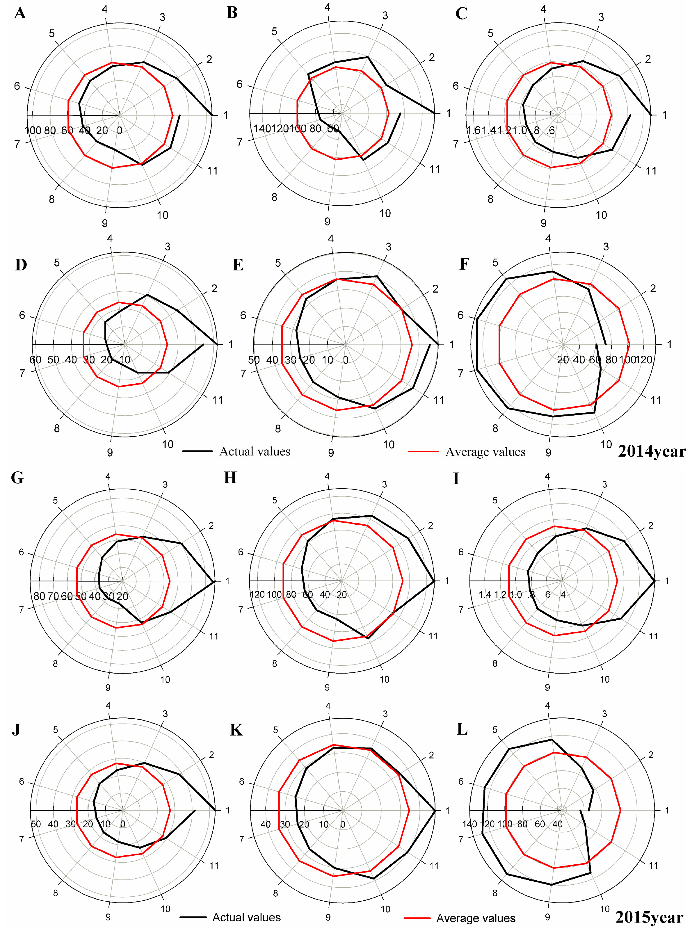
The average monthly concentrations of the principal air pollutants over China in 2014 are shown in Figure 2 and Table S1. The highest levels of PM2.5, PM10, CO, SO2, and NO2 were 106.5 μg/m−3, 154.1 μg/m−3, 1.69 mg/m−3, 62.0 μg/m−3, and 50.4 μg/m−3 in January. The lowest PM2.5 and PM10 levels were 39.8 μg/m−3 and 69.9 μg/m−3 in September, and the lowest values of CO, SO2, and NO2 were 0.93 mg/m−3, 19.7 μg/m−3, and 25.86 μg/m−3 in July. In contrast, the highest and lowest levels of O3 were 131.6 μg/m−3 in July and 61.3 μg/m−3 in December.
A comparison of the average monthly concentrations of PM2.5, PM10, CO, SO2, and NO2 indicated that the values were higher in January, February, November, and December, followed by March, April, May, and October, with lower concentrations from June to September. However, the opposite trend was observed with O3, which had the highest average monthly levels from May to August, followed by March, April, September, and October, with lower values in January, February, November, and December. Further, the highest PM2.5, PM10, CO, SO2, and NO2 levels were higher than the lowest ones, respectively, indicating that the principal air pollutants were highest in January.
Similar trends were observed in 2015 (Figure 2). The highest levels of PM2.5, PM10, CO, and NO2 were 86.8 μg/m−3, 129.3 μg/m−3, 1.60 mg/m−3, and 48.0 μg/m−3 in December, and the highest levels of SO2 and O3 were 53.3 μg/m−3 in January and 130.8 μg/m−3 in August (Table S1). The lowest PM2.5 and PM10 levels were 36.4 μg/m−3 and 65.4 μg/m−3 in September, and the lowest values of CO, SO2, and NO2 were 0.83 mg/m−3, 15.7 μg/m−3, and 24.4 μg/m−3 in July. The lowest level of O3 was 55.7 μg/m−3 in August (Table S1).
The average monthly PM2.5, PM10, CO, SO2, and NO2 concentrations in January and December were higher than in other months. Thus, the highest PM2.5, PM10, CO, SO2, and NO2 levels were 2.38, 1.98, 1.91, 3.39, 1.97, and 2.35 times greater than the lowest ones. However, the average monthly concentration of O3 was higher from May to August, followed by March, April, September, and October, with lower values found from January to December.
3.2. Spatial Analysis of the Principal Air Pollutants
We obtained the average concentrations of the principal air pollutants during the four months (January, February, November, and December), except for O3, the average value of which was calculated from May to August. Following the processes described above, we measured the spatial distribution of the principal air pollutants in 2014 (Figure 3). The highest and lowest levels of PM2.5 and PM10 were 191.4 μg/m−3 and 296.9 μg/m−3 in Baoding, and 26.4 μg/m−3 and 44.5 μg/m−3 in Sanya (Table S2). The provinces of Shanxi, Shandong, Henan, and Shanxi, and the Beijing-Tianjin-Hebei region were the most polluted. It should be noted that most areas of China were affected by PM2.5 and PM10, including central and northern China. With respect to CO, SO2, NO2, and O3, the distribution narrowed, and was more centralized in the Beijing-Tianjin-Hebei region, and Shandong and Henan provinces. The highest values of CO, SO2, NO2, and O3 were 3.62 mg/m−3 in Baoding, 151.5 μg/m−3 in Yangquan, 85.2 μg/m−3 in Baoding, and 225.2 μg/m−3 in Wuhan (Table S2), respectively.
The air quality improved in 2015 in comparison to 2014 (Figure 3). The most polluted areas were primarily in the provinces of Hebei, Shandong, and Henan, with the highest levels of PM2.5, PM10, and CO (170.4 μg/m−3, 254.2 μg/m−3, and 3.57 mg/m−3) in Baoding (Table S2). The highest values of SO2, NO2, and O3 were 137.0 μg/m−3 in Shenyang, 77 μg/m−3 in Xingtai, and 184.6 μg/m−3 in Dezhou (Table S2), respectively. The lowest values of the principal air pollutants were observed in Hainan province.
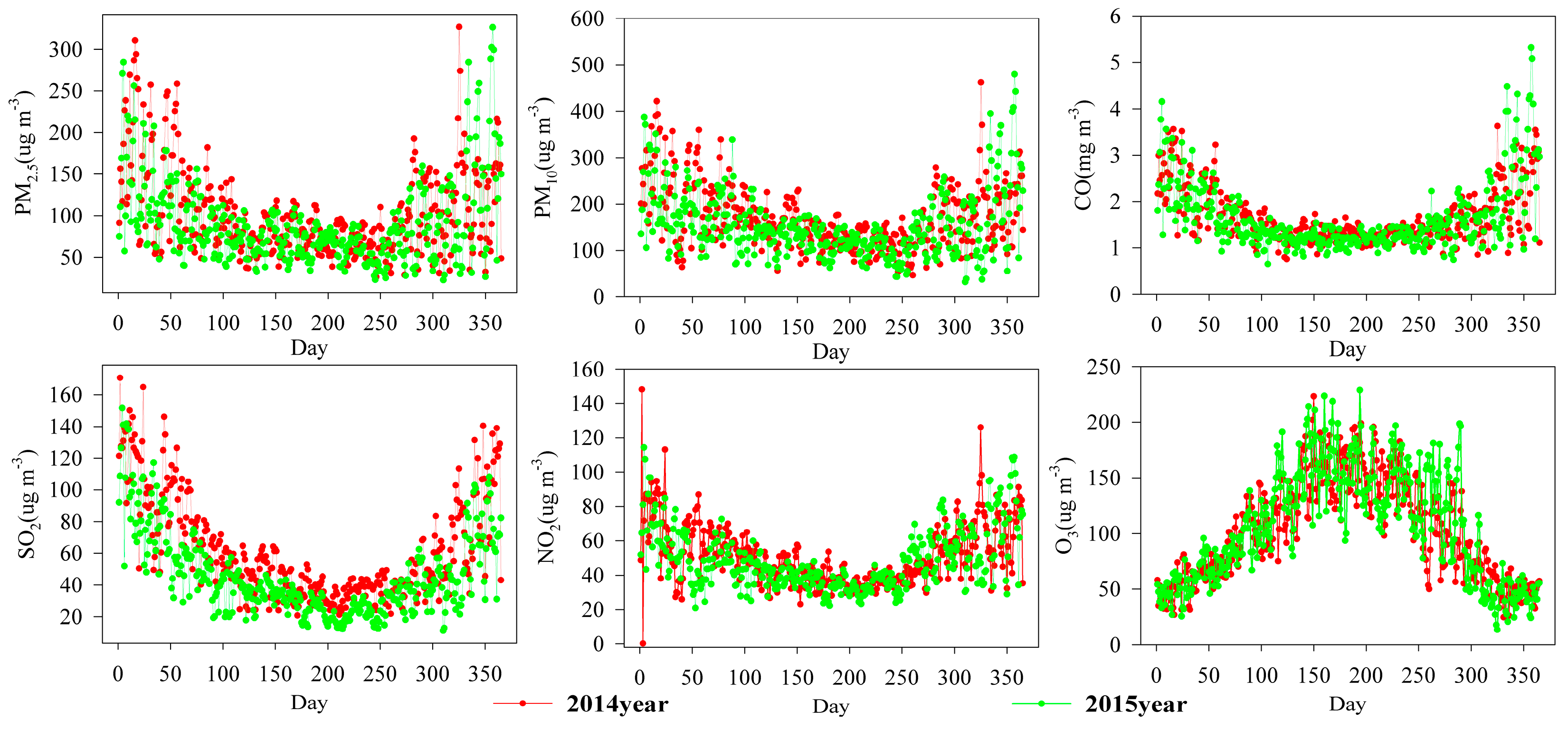
The dynamic and spatiotemporal distribution of the principal air pollutants indicated that the cities Baoding, Xingtai, Handan, Shijiazhuang, Hengshui, Dezhou, Tangshan, Heze, Langfang, Liaocheng, Zibo, Laiwu, Anyang, Linyi, Yichang, Zhengzhou, and Pingdingshan were the most polluted regions; hence, the average daily concentrations of the principal air pollutants were analyzed in 2014 and 2015 (Figure 4). The average daily concentrations of air pollutants (SO2, NO2, CO, PM2.5, and PM10) were also higher in the spring and winter, except for O3, which had the higher average daily levels in the summer. Besides, the average daily concentrations of SO2, NO2, CO, PM2.5, and PM10 decreased at a rate of 16.2 (μg/m−3)/year, 2.8 (μg/m−3)/year, 0.1 (mg/m−3)/year, 11.8 (μg/m−3)/year, and 17.8 (μg/m−3)/year from 2014 to 2015, respectively. On the contrary, the average daily concentrations of O3 increased from 102.2 (μg/m−3)/year to 105.4 (μg/m−3)/year between 2014 and 2015.
3.3. The Dynamics of the Principal Air Pollutants in Beijing-Tianjin-Hebei during January, February, November, and December
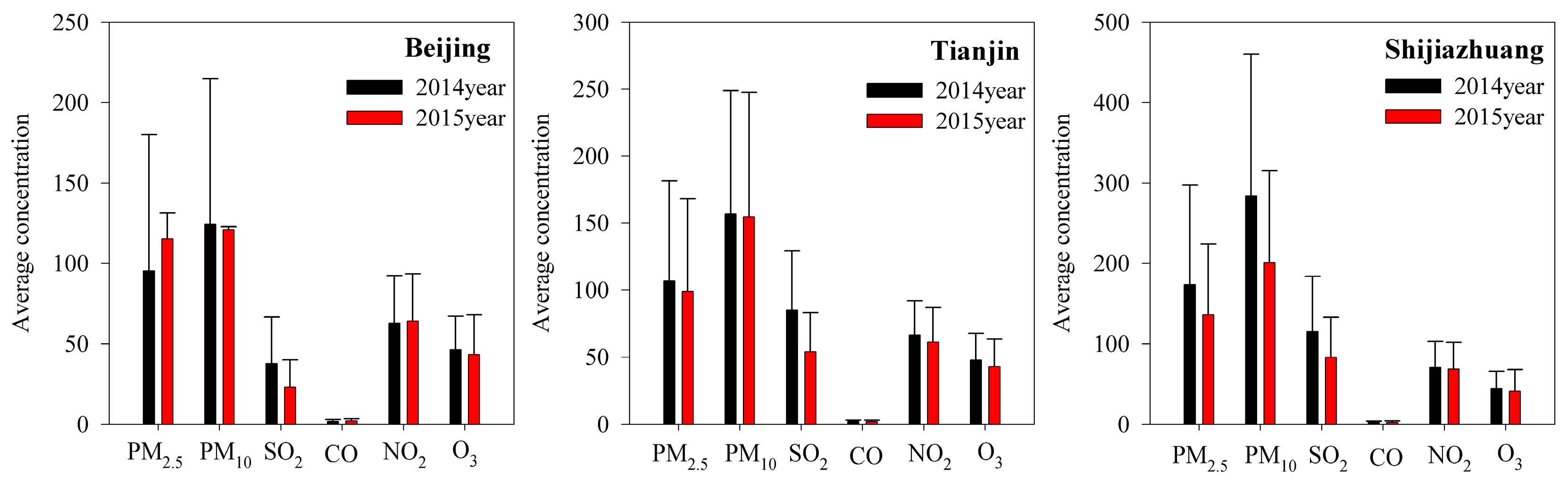
As for the mosted polluteted region (Beijing-Tianjin-Hebei), Figure 5 exhibits the dynamic of the principal air pollutants during January, February, November, and December in 2014 and 2015. In Beijing, the concentrations of PM2.5, CO, and NO2 slightly increased; while the concentrations of PM10, SO2, and O3 decreased at a rate of 3.5 (μg/m−3)/year, 14.7 (μg/m−3)/year, and 3.0 (μg/m−3)/year, respectively. All the principal air pollutants in Tianjin showed a decreasing trend, especially for the SO2, which decreased at a rate of 30.9 (μg/m−3)/year. Similarly, all the principal air pollutants in Shijiazhuang also decreased, except for the CO, which increased at a rate of 0.1 (mg/m−3)/year. In addition, the concentration of PM10 obviously decreased at a rate of 83.1 (μg/m−3)/year in Shijiazhuang.
3.4. The Dynamics of the Principal Air Pollutants in Shandong, Henan, and Hebei during Autumn
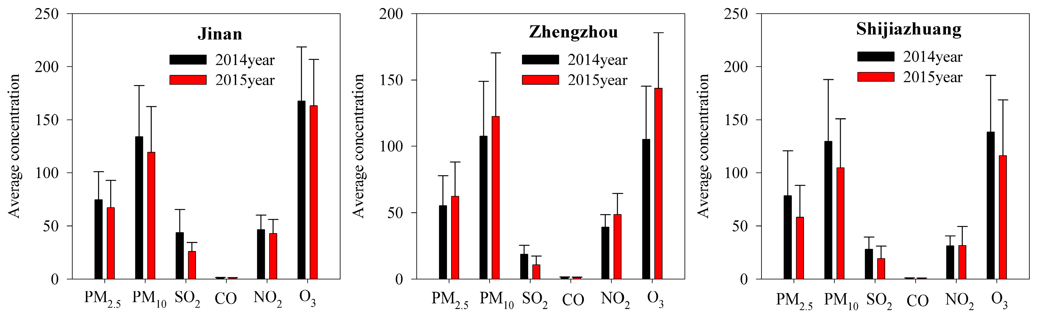
In terms of the major agricultural provinces Shandong, Henan, and Hebei, the dynamics of the principal air pollutants in Jinan and Zhengzhou during July and September are presented in Figure 6. In Jinan, all the principal air pollutants showed a decreasing trend, especially for SO2, which decreased at a rate of 18.0 (μg/m−3)/year. However, the average concentrations of PM2.5, PM10, NO2, and O3 in Zhengzhou increased at a rate of 7.0 (μg/m−3)/year, 14.7 (μg/m−3)/year, 9.4 (μg/m−3)/year, and 38.6 (μg/m−3)/year, respectively. Fortunately, the concentration of SO2 and CO presented a decreasing trend in Zhengzhou during autumn. In addition, all the principal air pollutants in Shijiazhuang also decreased, except for the NO2, which slightly increased at a rate of 0.4 (μg/m−3)/year.
3.5. The Relationships among the Principal Air Pollutants
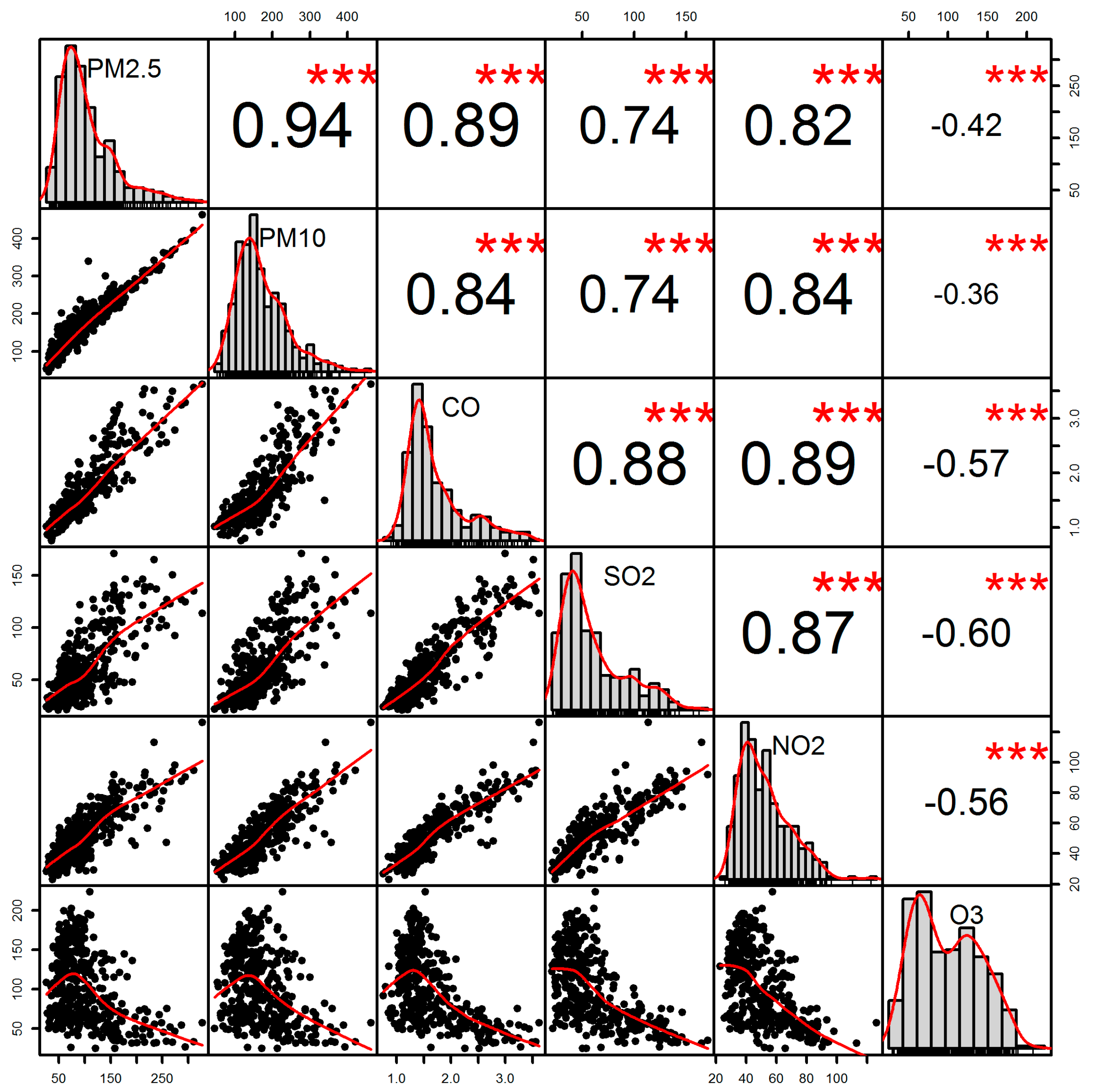
As Figure 7 shows, the correlation coefficients among air pollutants were significant at p < 0.05 in the most polluted 17 cities (2014). Our results indicated that there were positive correlations among PM2.5, PM10, CO, SO2, and NO2, and negative correlations for O3. As for PM2.5, and the correlation coefficients between PM10, CO, SO2, NO2, and O3 were 0.94, 0.89, 0.74, 0.82, and −0.42, respectively. High correlation coefficients among CO, SO2, and NO2 (0.88 for CO and SO2, 0.89 for CO and NO2, 0.87 for SO2 and NO2) were observed. We also found significant negative correlation coefficients among O3, CO, SO2, and NO2 (−0.57 for O3 and CO, −0.60 for O3 and SO2, and −0.56 for O3 and NO2).
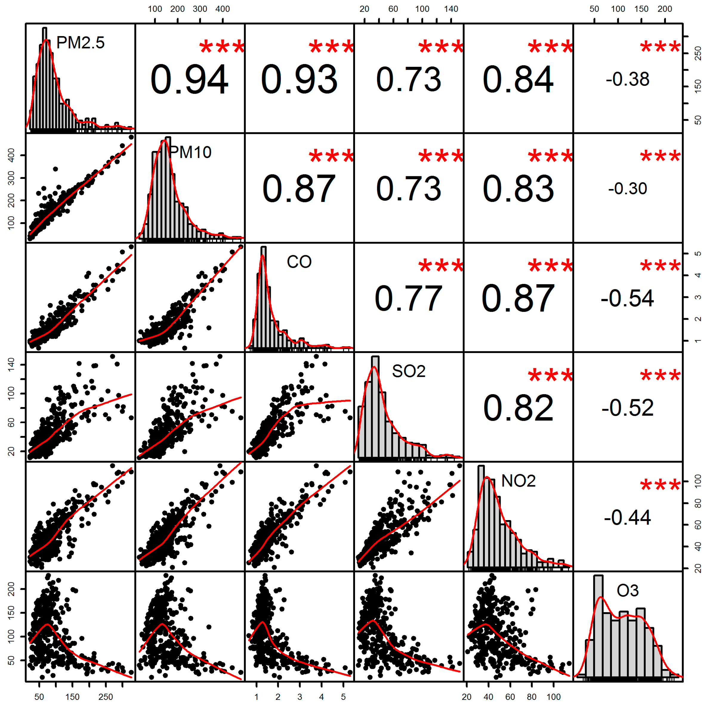
Figure 8 shows that there were significant relationships among the principal air pollutants in 2015. The correlation coefficients between PM2.5 and PM10, CO, SO2, NO2, and O3 were 0.94, 0.93, 0.73, 0.84, and −0.38. In addition, there was a slight decrease in the correlation coefficients among CO, SO2, and NO2 compared to those in 2014, with values of 0.77 for CO and SO2, 0.87 for CO and NO2, and 0.82 for SO2 and NO2. A similar decrease in the correlation coefficients among O3, CO, SO2, and NO2 was observed (−0.54 for O3 and CO, −0.52 for O3 and SO2, and −0.44 for O3 and NO2).
3.6. GAM Prediction of the Trend for Principal Air Pollutants
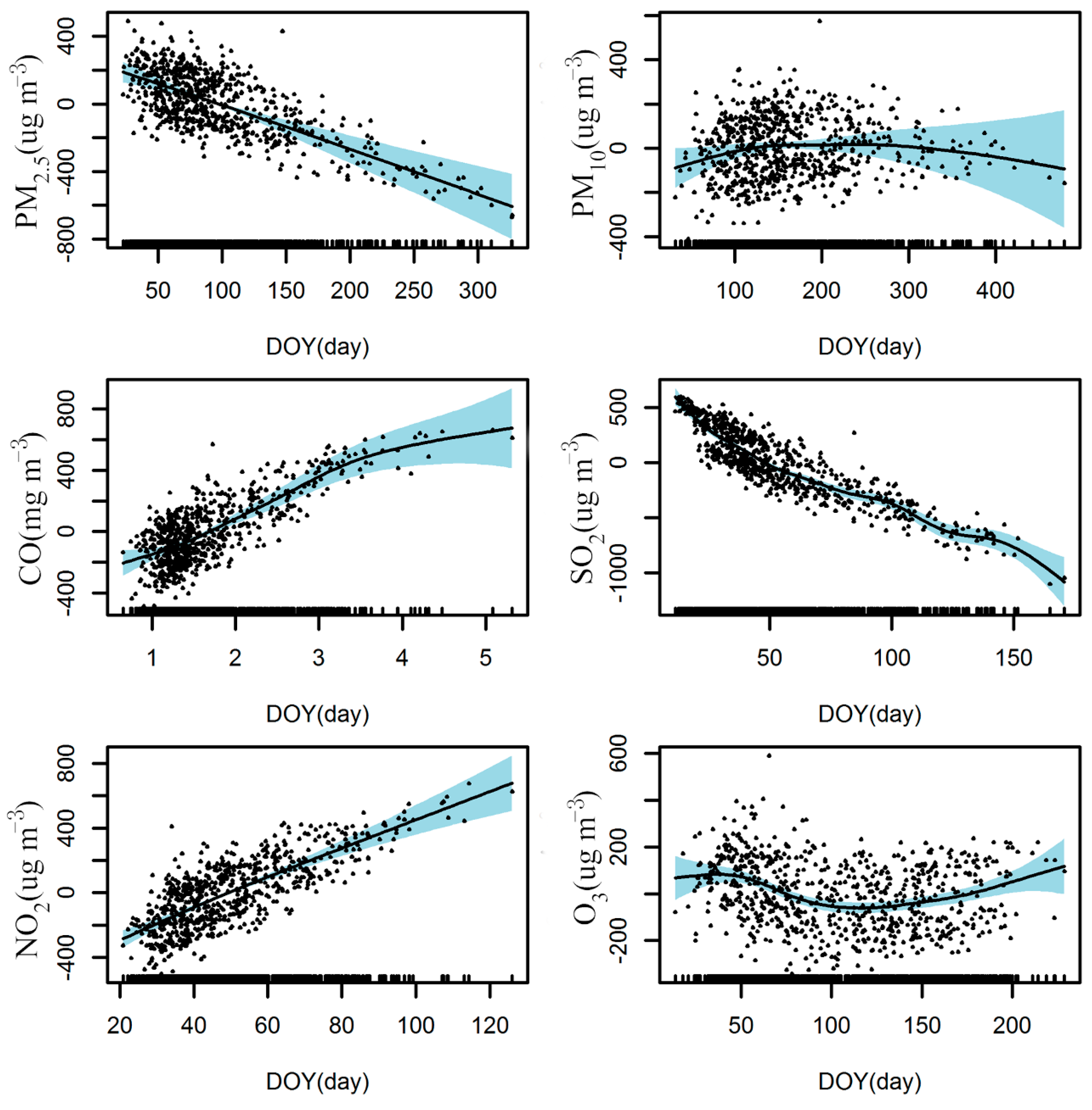
The GAM was employed to reveal the future dynamics of atmospheric pollutants (Figure 9), and the non-linear relationship between the pollutants and day-of-year trends was modeled flexibly by the log link function. The results showed that although PM2.5 and SO2 will decrease sharply in the future, further observation is imperative. Unfortunately, a consistent increase in NO2 and CO was predicted. Furthermore, a slight increase of PM10 was observed until it peaked between 100 < x < 150, and then decreased slightly over the remaining days. Meanwhile, the estimated O3 showed a slight increase before x = 50 and then decreased until approximately x = 125, followed by a slight upward trend during the remaining days. In summary, a small variation in PM10 and O3 indicated that the simulated results were reliable and desirable.
4. Discussion
4.1. Temporal and Spatial Patterns of China’s Principal Air Pollutants
The concentration of the principal air pollutants was higher in January and December—a phenomenon also observed in Fuzhou [45] and Shanghai [46,47]. In January 2013, two severe air pollution events happened in Beijing, during which the hourly concentration of PM2.5 rose to 680 µg/m−3 and 530 µg/m−3, respectively [38]. In Shanghai, the highest and lowest levels of PM10, NO2, and SO2 were found in winter and autumn, with vehicle emissions and meteorological conditions the most probable causes [36]. In the North China Plain, high emissions of atmospheric contamination, biomass burning, and stable weather conditions contributed to the haze events in winter [48], and higher energy consumption and motor vehicle emissions occurred in winter in Guangzhou [49]. If natural gas is supplied for municipal heating in Beijing rather than coal, air pollutant emissions (PM2.5, SO2, NOX, etc.) would decrease by 52% in winter [50] because the inter-transport of pollution and the secondary aerosols O3, OC (organic carbon) and VOC (volatile organic compounds) promote pollution. Thus, reducing the levels of air pollutants during the cold season is imperative for public health [51].
The spatial patterns of the average monthly simulation values indicated that in 2014 the most polluted regions were the Beijing-Tianjin-Hebei region and the provinces of Shanxi, Shandong, Henan, Hubei, and Shanxi. Industrial and domestic sources of pollution and agricultural emissions are the chief regional contributors to pollution in these regions [52]. Compared to 2014, the distribution patterns of air pollutants show a slight shift towards a smaller area in 2015, becoming more centralized in Hebei, Shandong, and Henan provinces, where haze episodes were also more frequent. A similar situation prevailed in the North China Plain [53], Guangzhou [22], and the Yangtze River Delta [26,54]. The stricter laws protecting air quality by government may account for this decreasing trend between 2014 and 2015 to some extent.
The significant relationships among air pollutants illustrated that there could be similar or interacting sources for the pollutions. Many studies have been undertaken to explore the source of large areas of haze. Biomass open burning contributes 47% of the PM2.5 in the Yangtze River Delta [55], is an important precursor for O3 [56], and is a stressor on marine ecosystems [57]. The fact that the inter-transport of pollution accompanies high humidity is the dominant reason for the haze in East China [29,46] and Northern Taiwan [27]. Dust was a major source of pollution in eastern Inner Mongolia [58], local emissions and regional transport accounted for pollution in Nanjing [59], coal consumption and industry increased pollution in Beijing in winter [32,50], and industrial pollution and vehicle emissions were the dominant local contributors to the levels of NO2 and PM2.5 in Shanghai [31,34].
Specifically, for the most polluted region—the northeast of China—the mineral dust from the deserts of western China contributes significantly to the concentration of PM [60,61]. The long-range transport dust plumes mixed with regional pollutants aid the formation of haze episodes [53,60,61,62]. Thus, the local pollutants also have significant contributions to the widespread haze pollution [48]. Meanwhile, during haze episodes, the secondary inorganic pollutants evident increased in PM [36], suggesting a joint effect among them [63]. Under unfavorable meteorological conditions, the interaction of PM and the secondary inorganic pollutants produced a large amount of aerosols with the characteristic of low visibility [36].
In general, the dust, municipal heating, and vehicle and local emissions are the dominant contributors to haze in winter [31], and meteorological conditions contribute significantly in the distribution, formation, and evolution of haze: for example, higher relative humidity and weaker wind speed contribute to haze [23,25,30]. In addition, there is a positive relationship between visibility and wind speed, and a negative relationship with relative humidity [45,49,59]. Secondary inorganic ions were also positively correlated with stable weather conditions (higher relative humidity), which determined the specific chemical composition of haze [64]. In summary, the median or highest values and the distribution area of air pollutants showed a decreasing trend from 2014 to 2015, which may be explained in part by the improved energy efficiency and stricter laws protecting air quality.
4.2. Policy Recommendations
The estimated values of PM2.5 and SO2 showed a sharp decreasing trend. However, we observed a consistent increasing trend in CO and NO2, while the estimated values of PM10 and O3 remained stable overall. Thus, the concentration of CO and NO2 in China will continue to increase. As we know already, vehicle emissions are a key factor in the high concentration of NO2, which has been caused by the rapid increase in the number of vehicles and industrial parks [31,34]. Therefore, technological innovation is imperative in coal gasification, liquefaction, and storage to improve the energy efficiency of coal [65]. Indeed, replacing fossil fuels with clean fuel (natural gas, nuclear energy, etc.) for municipal heating in winter would be an effective long-term measure to mitigate the dense haze north of the Yellow River [50]. In addition, stringent measures to control particle emissions (biomass burning) should be implemented during specific periods based on meteorological conditions [29,66], while mass transit should be encouraged to avoid energy waste. Further, the central and local government should subsidize the manufacture of hybrid, flex-fuel, and electric automobiles [67,68], and remove market-entry barriers to promote competition among companies [65]. Finally, we need to improve the proportion of the tertiary industry to optimize the economic structure that uses less energy and produces fewer particle emissions [69,70].
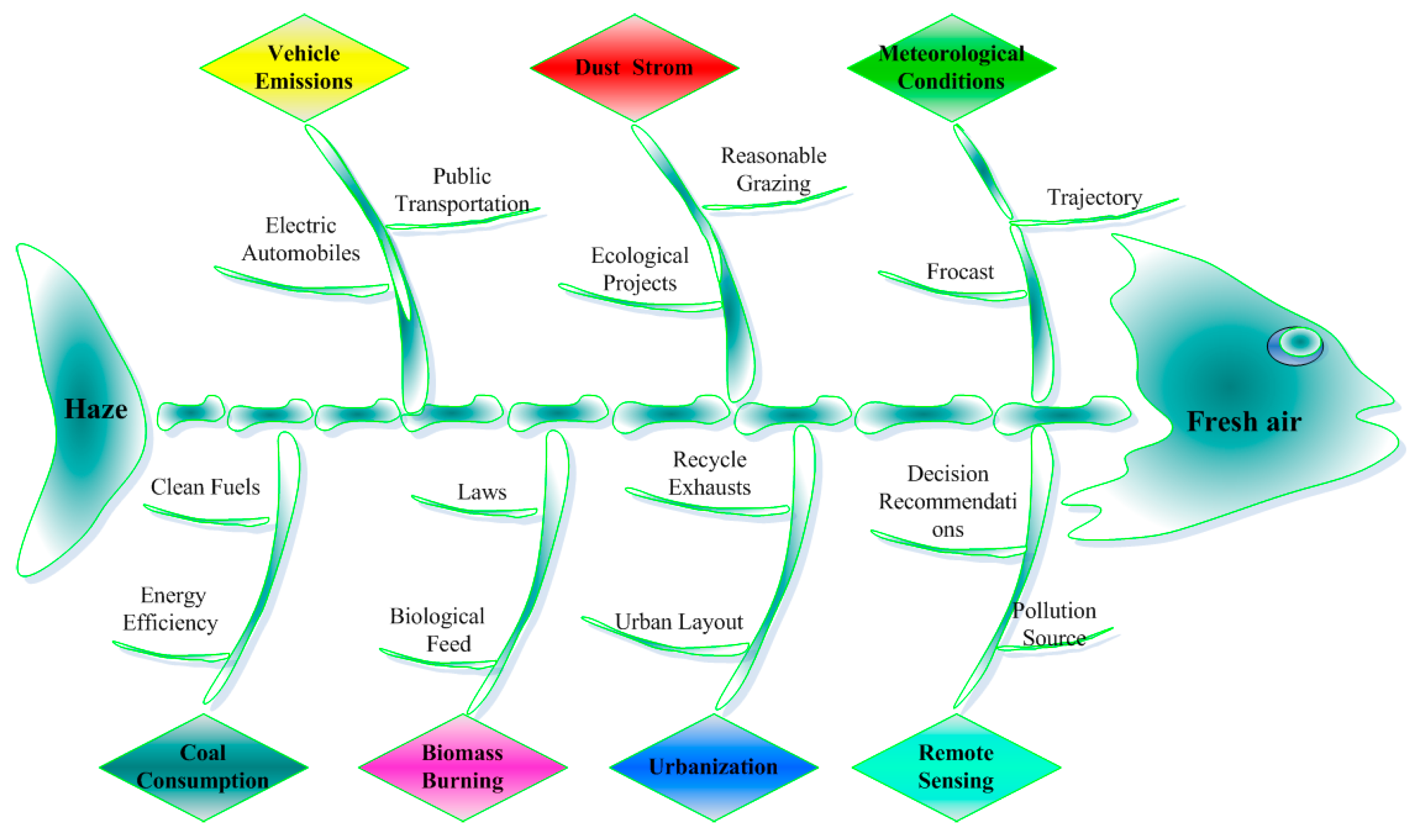
As Figure 10 shows, this study highlighted the measures needed to decrease current sources of air pollutants. Indeed, replacing fossil fuels with clean fuels (natural gas, nuclear, wind, and solar energy) will help to address air pollution’s root causes. To transform and improve air quality, restricting biomass burning during specific periods (according to meteorological conditions) is imperative, and it may be necessary to implement strict environmental policies forbidding open biomass burning when municipal heating is highest. We should also consider recycling biological feed. Equally important, the issue of vehicle emissions requires the cooperation of government, manufacturers, retailers, and consumers—particularly in the development and promotion of flex-fuel (hybrid) and electric automobiles. Further, ecosystem restoration projects such as the Three-North Shelterbelt System can be effective in defending against sandstorms while simultaneously improving the regional environment. Remote sensing should also be employed to monitor the formation and development of haze, to record, measure, and evaluate the sources of pollution, and monitor the trajectory of haze over the long-term. Indeed, predicting the values and levels of air pollutants and communicating this information by mobile messages will cement trust between individuals and governments. Further, analyzing the structure and function of cities based on local conditions to facilitate scientific urban planning and formulate reasonable population distribution policies should help to mitigate pollution. All of the aforementioned underscore the essential need to share information, provide support, and increase cooperation among different departments to achieve effective haze control. Of course, trade-offs between environmental objectives, economic growth, energy consumption, living standards, and funding are inevitable, but we believe that these can be balanced for the benefit and welfare of all.
5. Conclusions
Because particulate haze episodes over China have increased in recent years, it is imperative that we understand pollutant pathways and propose recommendations for a policy framework. In general, November to February demonstrated the highest concentrations of air pollutants (PM2.5, PM10, CO, SO2, and NO2), excluding O3 levels, which were highest from May to August. Further, the most highly polluted areas were in the provinces of Shandong, Henan, and Shanxi, and in the Beijing-Tianjin-Hebei region. Fortunately, most of the principal air pollutants presented a decreasing or relatively stable trend in Beijing-Tianjin-Hebei during January, February, November, and December. Meanwhile, most of the principal air pollutants also presented a decreasing trend in Jinan and Shijiazhuang in autumn. However, in Zhengzhou, the haze events during autumn were unoptimistic. Although the conflict between clean air and economic growth will continue, measures can be taken to mitigate the sources of air pollutants and to use resources to control, reduce, and manage air pollution.
To improve our understanding of the formation and frequency of haze, satellite observations and monitoring of high-risk areas are important subjects for future research. We need to understand the specific effects of meteorological conditions on the transport mechanism of air pollutants, and the role they play in the secondary formation process.
Supplementary Materials
The following are available online at www.mdpi.com/2073-4433/8/8/137/s1: Table S1: The average monthly concentration of air pollutants over China during 2014 and 2015; Table S2: The mean concentration of air pollutants over China among four months (January, February, November, and December).
Acknowledgments
This work was supported by the Ministry of Environmental Protection of the People’s Republic of China. The research was funded as well by the West Light Foundation of The Chinese Academy of Sciences, and the Open Fund of the Key Laboratory of Mountain Surface Processes and Eco-regulation.
Author Contributions
J.S. contributed to the study design, J.S., T.Z. and H.Y. were involved in drafting the manuscript, approving the final draft, and agree to be accountable for the work. All authors read and approved the final manuscript.
Conflicts of Interest
The authors declare no conflict of interest.
References
- He, X.Y.; Hu, J.B.; Chen, W.; Li, X.Y. Haze removal based on advanced haze-optimized transformation (AHOT) for multispectral imagery. Int. J. Remote Sens. 2010, 31, 5331–5348. [Google Scholar] [CrossRef]
- Han, L.J.; Zhou, W.Q.; Pickett, S.T.A.; Li, W.F.; Li, L. An optimum city size? The scaling relationship for urban population and fine particulate (PM2.5) concentration. Environ. Pollut. 2016, 208, 96–101. [Google Scholar] [CrossRef] [PubMed]
- Carrasco, L.R. Silver lining of Singapore’s haze. Science 2013, 341, 342–343. [Google Scholar] [CrossRef] [PubMed]
- Hao, Y.; Liu, Y.-M. The influential factors of urban PM2.5 concentrations in China: A spatial econometric analysis. J. Clean. Prod. 2016, 112, 1443–1453. [Google Scholar] [CrossRef]
- Malandrino, M.; Casazza, M.; Abollino, O.; Minero, C.; Maurino, V. Size resolved metal distribution in the PM matter of the city of Turin (Italy). Chemosphere 2016, 147, 477–489. [Google Scholar] [CrossRef] [PubMed]
- Salinas, S.V.; Chew, B.N.; Miettinen, J.; Campbell, J.R.; Welton, E.J.; Reid, J.S.; Yu, L.Y.E.; Liew, S.C. Physical and optical characteristics of the October 2010 haze event over Singapore: A photometric and lidar analysis. Atmos. Res. 2013, 122, 555–570. [Google Scholar] [CrossRef]
- Kim, K.W.; Kim, Y.J.; Bang, S.Y. Summer time haze characteristics of the urban atmosphere of Gwangju and the rural atmosphere of Anmyon, Korea. Environ. Monit. Assess. 2008, 141, 189–199. [Google Scholar] [CrossRef] [PubMed]
- Zhao, H.M.; Zhang, X.L.; Zhang, S.C.; Chen, W.W.; Tong, D.Q.; Xiu, A.J. Effects of Agricultural Biomass Burning on Regional Haze in China: A Review. Atmosphere 2017, 8, 88. [Google Scholar] [CrossRef]
- Szidat, S. Atmosphere. Sources of Asian Haze. Science 2009, 323, 470–471. [Google Scholar] [CrossRef] [PubMed]
- Begum, B.A.; Hopke, P.K. Identification of haze-creating sources from fine particulate matter in Dhaka aerosol using carbon fractions. J. Air Waste Manag. 2013, 63, 1046–1057. [Google Scholar] [CrossRef]
- Pernigotti, D.; Belis, C.A.; Spano, L. Specieurope: The European data base for PM source profiles. Atmos. Pollut. Res. 2016, 7, 307–314. [Google Scholar] [CrossRef]
- Huang, R.J.; Zhang, Y.; Bozzetti, C.; Ho, K.F.; Cao, J.J.; Han, Y.; Daellenbach, K.R.; Slowik, J.G.; Platt, S.M.; Canonaco, F. High secondary aerosol contribution to particulate pollution during haze events in China. Nature 2014, 514, 218–222. [Google Scholar] [CrossRef] [PubMed] [Green Version]
- Soleiman, A.; Ohtman, M.; Samah, A.A.; Sulaiman, N.M.; Radojevic, M. The occurrence of haze in Malaysia: A case study in an urban industrial area. Pure Appl. Geophys. 2003, 160, 221–238. [Google Scholar] [CrossRef]
- Abdullaev, S.F.; Maslov, V.A.; Nazarov, B.I. Study of dust haze in arid zone. Izv. Atmos. Ocean. Phys. 2013, 49, 276–284. [Google Scholar] [CrossRef]
- Zhang, R.H.; Li, Q.; Zhang, R.N. Meteorological conditions for the persistent severe fog and haze event over eastern China in January 2013. Sci. China Earth Sci. 2014, 57, 26–35. [Google Scholar]
- Elias, T.; Haeffelin, M.; Drobinski, P.; Gomes, L.; Rangognio, J.; Bergot, T.; Chazette, P.; Raut, J.C.; Colomb, M. Particulate contribution to extinction of visible radiation: Pollution, haze, and fog. Atmos. Res. 2009, 92, 443–454. [Google Scholar] [CrossRef]
- Sun, J.; Zhou, T.C. Health risk assessment of China’s main air pollutants. BMC Public Health 2017, 17, 212. [Google Scholar] [CrossRef] [PubMed]
- Zhang, X.Y.; Wang, Y.Q.; Niu, T.; Zhang, X.C.; Gong, S.L.; Zhang, Y.M.; Sun, J.Y. Atmospheric aerosol compositions in China: Spatial/temporal variability, chemical signature, regional haze distribution and comparisons with global aerosols. Atmos. Chem. Phys. 2012, 12, 799. [Google Scholar]
- Wang, Y.; Li, Z.Q.; Zhang, Y.; Wang, Q.; Ma, J.Z. Impact of aerosols on radiation during a heavy haze event in Beijing. IOP Conf. Ser. Earth Environ. Sci. 2014, 17, 012012. [Google Scholar]
- Sun, Y.L.; Jiang, Q.; Wang, Z.F.; Fu, P.Q.; Li, J.; Yang, T.; Yin, Y. Investigation of the sources and evolution processes of severe haze pollution in Beijing in January 2013. J. Geophys. Res. Atmos. 2014, 119, 4380–4398. [Google Scholar] [CrossRef]
- Zhang, M.; Ma, Y.Y.; Gong, W.; Zhu, Z.M. Aerosol optical properties of a haze episode in Wuhan based on ground-based and satellite observations. Atmosphere 2014, 5, 699–719. [Google Scholar] [CrossRef]
- Zhang, Z.L.; Wang, J.; Chen, L.H.; Chen, X.Y.; Sun, G.Y.; Zhong, N.S.; Kan, H.D.; Lu, W.J. Impact of haze and air pollution-related hazards on hospital admissions in Guangzhou, China. Environ. Sci. Pollut. Res. 2014, 21, 4236–4244. [Google Scholar] [CrossRef] [PubMed]
- Liu, X.G.; Li, J.; Qu, Y.; Han, T.; Hou, L.; Gu, J.; Chen, C.; Yang, Y.; Liu, X.; Yang, T.; et al. Formation and evolution mechanism of regional haze: A case study in the megacity Beijing, China. Atmos. Chem. Phys. 2013, 13, 4501–4514. [Google Scholar] [CrossRef]
- Quan, J.; Zhang, Q.; He, H.; Liu, J.; Huang, M.; Jin, H. Analysis of the formation of fog and haze in North China Plain (NCP). Atmos. Chem. Phys. 2011, 11, 8205–8214. [Google Scholar] [CrossRef]
- Bei, N.F.; Xiao, B.; Meng, N.; Feng, T. Critical role of meteorological conditions in a persistent haze episode in the Guanzhong basin, China. Sci. Total Environ. 2016, 550, 273–284. [Google Scholar] [CrossRef] [PubMed]
- Tang, L.L.; Yu, H.X.; Ding, A.J.; Zhang, Y.J.; Qin, W.; Wang, Z.; Chen, W.T.; Hua, Y.; Yang, X.X. Regional contribution to PM1 pollution during winter haze in Yangtze River Delta, China. Sci. Total Environ. 2016, 541, 161–166. [Google Scholar] [CrossRef] [PubMed]
- Wang, S.H.; Hung, W.T.; Chang, S.C.; Yen, M.C. Transport characteristics of Chinese haze over Northern Taiwan in winter, 2005–2014. Atmos. Environ. 2016, 126, 76–86. [Google Scholar] [CrossRef]
- Gabrielli, M.; Fracassetti, D.; Tirelli, A. Release of phenolic compounds from cork stoppers and its effect on protein-haze. Food Control 2016, 62, 330–336. [Google Scholar] [CrossRef]
- Tao, M.H.; Chen, L.F.; Wang, Z.F.; Tao, J.H.; Su, L. Satellite observation of abnormal yellow haze clouds over East China during summer agricultural burning season. Atmos. Environ. 2013, 79, 632–640. [Google Scholar] [CrossRef]
- Sun, Y.; Song, T.; Tang, G.Q.; Wang, Y.S. The vertical distribution of PM2.5 and boundary-layer structure during summer haze in Beijing. Atmos. Environ. 2013, 74, 413–421. [Google Scholar] [CrossRef]
- Wang, Y.J.; Li, L.; Chen, C.H.; Huang, C.; Huang, H.Y.; Feng, J.L.; Wang, S.X.; Wang, H.L.; Zhang, G.; Zhou, M.; et al. Source apportionment of fine particulate matter during autumn haze episodes in Shanghai, China. J. Geophys. Res. Atmos. 2014, 119, 1903–1914. [Google Scholar] [CrossRef]
- Lin, Y.C.; Hsu, S.C.; Chou, C.C.K.; Zhang, R.J.; Wu, Y.F.; Kao, S.J.; Luo, L.; Huang, C.H.; Lin, S.H.; Huang, Y.T. Wintertime haze deterioration in Beijing by industrial pollution deduced from trace metal fingerprints and enhanced health risk by heavy metals. Environ. Pollut. 2016, 208, 284–293. [Google Scholar] [CrossRef] [PubMed]
- Gui, K.; Che, H.Z.; Chen, Q.L.; An, L.C.; Zeng, Z.L.; Guo, Z.Y.; Zheng, Y.; Wang, H.; Wang, Y.Q.; Yu, J.; et al. Aerosol optical properties based on ground and satellite retrievals during a serious haze episode in December 2015 over Beijing. Atmosphere 2016, 7, 70. [Google Scholar] [CrossRef]
- Zhao, W.C.; Cheng, J.P.; Li, D.L.; Duan, Y.S.; Wei, H.P.; Ji, R.X.; Wang, W.H. Urban ambient air quality investigation and health risk assessment during haze and non-haze periods in Shanghai, China. Atmos. Pollut. Res. 2013, 4, 275–281. [Google Scholar] [CrossRef]
- Li, W.J.; Shi, Z.B.; Zhang, D.Z.; Zhang, X.Y.; Li, P.R.; Feng, Q.J.; Yuan, Q.; Wang, W.X. Haze particles over a coal-burning region in the China Loess Plateau in winter: Three flight missions in December 2010. J. Geophys. Res. Atmos. 2012, 117. [Google Scholar] [CrossRef]
- Zhao, X.J.; Zhao, P.S.; Xu, J.; Meng, W.; Pu, W.W.; Dong, F.; He, D.; Shi, Q.F. Analysis of a winter regional haze event and its formation mechanism in the North China Plain. Atmos. Chem. Phys. 2013, 13, 5685–5696. [Google Scholar] [CrossRef]
- Zhu, C.S.; Cao, J.J.; Tsai, C.J.; Shen, Z.X.; Liu, S.X.; Huang, R.J.; Zhang, N.N.; Wang, P. The rural carbonaceous aerosols in coarse, fine, and ultrafine particles during haze pollution in northwestern China. Environ. Sci. Pollut. Res. 2016, 23, 4569–4575. [Google Scholar] [CrossRef] [PubMed]
- Wang, Y.S.; Yao, L.; Wang, L.L.; Liu, Z.R.; Ji, D.S.; Tang, G.Q.; Zhang, J.K.; Sun, Y.; Hu, B.; Xin, J.Y. Mechanism for the formation of the January 2013 heavy haze pollution episode over central and eastern China. Sci. China Earth Sci. 2014, 57, 14–25. [Google Scholar] [CrossRef]
- Zhu, T.; Shang, J.; Zhao, D.F. The roles of heterogeneous chemical processes in the formation of an air pollution complex and gray haze. Sci. China Chem. 2011, 54, 145–153. [Google Scholar] [CrossRef]
- Jansen, R.C.; Shi, Y.; Chen, J.M.; Hu, Y.J.; Xu, C.; Hong, S.M.; Li, J.; Zhang, M. Using hourly measurements to explore the role of secondary inorganic aerosol in PM2.5 during haze and fog in Hangzhou, China. Adv. Atmos. Sci. 2014, 31, 1427–1434. [Google Scholar] [CrossRef]
- Shen, X.J.; Sun, J.Y.; Zhang, X.Y.; Zhang, Y.M.; Zhang, L.; Che, H.C.; Ma, Q.L.; Yu, X.M.; Yue, Y.; Zhang, Y.W. Characterization of submicron aerosols and effect on visibility during a severe haze-fog episode in Yangtze River Delta, China. Atmos. Environ. 2015, 120, 307–316. [Google Scholar] [CrossRef]
- Lin, Y.F.; Huang, K.; Zhuang, G.S.; Fu, J.S.; Wang, Q.Z.; Liu, T.N.; Deng, C.R.; Fu, Q.Y. A multi-year evolution of aerosol chemistry impacting visibility and haze formation over an Eastern Asia megacity, Shanghai. Atmos. Environ. 2014, 92, 76–86. [Google Scholar] [CrossRef]
- Catalano, M.; Galatioto, F.; Bell, M.; Namdeo, A.; Bergantino, A.S. Improving the prediction of air pollution peak episodes generated by urban transport networks. Environ. Sci. Policy 2016, 60, 69–83. [Google Scholar] [CrossRef]
- Chen, X.L.; Feng, Y.R.; Li, J.N.; Lin, W.S.; Fan, S.J.; Wang, A.Y.; Fong, S.K.; Lin, H. Numerical simulations on the effect of sea-land breezes on atmospheric haze over the Pearl River Delta Region. Environ. Model. Assess. 2009, 14, 351–363. [Google Scholar]
- Zhang, F.W.; Xu, L.L.; Chen, J.S.; Chen, X.Q.; Niu, Z.C.; Lei, T.; Li, C.M.; Zhao, J.P. Chemical characteristics of PM2.5 during haze episodes in the urban of Fuzhou, China. Particuology 2013, 11, 264–272. [Google Scholar] [CrossRef]
- Wang, X.M.; Chen, J.M.; Cheng, T.T.; Zhang, R.Y.; Wang, X.M. Particle number concentration, size distribution and chemical composition during haze and photochemical smog episodes in Shanghai. J. Environ. Sci. 2014, 26, 1894–1902. [Google Scholar] [CrossRef] [PubMed]
- Wang, H.L.; Qiao, L.P.; Lou, S.R.; Zhou, M.; Ding, A.J.; Huang, H.Y.; Chen, J.M.; Wang, Q.; Tao, S.K.; Chen, C.H.; et al. Chemical composition of PM2.5 and meteorological impact among three years in urban Shanghai, China. J. Clean. Prod. 2016, 112, 1302–1311. [Google Scholar] [CrossRef]
- Gao, M.; Carmichael, G.R.; Wang, Y.; Saide, P.E.; Yu, M.; Xin, J.; Liu, Z.; Wang, Z. Modeling study of the 2010 regional haze event in the North China Plain. Atmos. Chem. Phys. 2016, 16, 1673–1691. [Google Scholar] [CrossRef]
- Tan, J.H.; Duan, J.C.; Chen, D.H.; Wang, X.H.; Guo, S.J.; Bi, X.H.; Sheng, G.Y.; He, K.B.; Fu, J.M. Chemical characteristics of haze during summer and winter in Guangzhou. Atmos. Res. 2009, 94, 238–245. [Google Scholar] [CrossRef]
- Li, H.C.; Yang, S.Y.; Zhang, J.; Qian, Y. Coal-based synthetic natural gas (SNG) for municipal heating in China: Analysis of haze pollutants and greenhouse gases (GHGs) emissions. J. Clean. Prod. 2016, 112, 1350–1359. [Google Scholar] [CrossRef]
- Fang, Z.Q.; Zhu, H.L.; Bao, W.Z.; Preston, C.; Liu, Z.; Dai, J.Q.; Li, Y.Y.; Hu, L.B. Highly transparent paper with tunable haze for green electronics. Energ. Environ. Sci. 2014, 7, 3313–3319. [Google Scholar] [CrossRef]
- Wang, L.T.; Wei, Z.; Yang, J.; Zhang, Y.; Zhang, F.F.; Su, J.; Meng, C.C.; Zhang, Q. The 2013 severe haze over southern Hebei, China: Model evaluation, source apportionment, and policy implications. Atmos. Chem. Phys. 2014, 14, 3151–3173. [Google Scholar] [CrossRef] [Green Version]
- Zhang, X.L.; Huang, Y.B.; Zhu, W.Y.; Rao, R.Z. Aerosol characteristics during summer haze episodes from different source regions over the coast city of North China Plain. J. Quant. Spectrosc. Radiat. Transf. 2013, 122, 180–193. [Google Scholar] [CrossRef]
- Wang, S.; Zhou, C.; Wang, Z.; Feng, K.; Hubacek, K. The characteristics and drivers of fine particulate matter (PM2.5) distribution in China. J. Clean. Prod. 2017, 142, 1800–1809. [Google Scholar] [CrossRef]
- Cheng, Z.; Wang, S.; Fu, X.; Watson, J.G.; Jiang, J.; Fu, Q.; Chen, C.; Xu, B.; Yu, J.; Chow, J.C.; et al. Impact of biomass burning on haze pollution in the Yangtze River delta, China: A case study in summer 2011. Atmos. Chem. Phys. 2014, 14, 4573–4585. [Google Scholar] [CrossRef] [Green Version]
- Zhang, Y.W.; Zhang, X.Y.; Zhang, Y.M.; Shen, X.J.; Sun, J.Y.; Ma, Q.L.; Yu, X.M.; Zhu, J.L.; Zhang, L.; Che, H.C. Significant concentration changes of chemical components of PM1 in the Yangtze River Delta area of China and the implications for the formation mechanism of heavy haze-fog pollution. Sci. Total Environ. 2015, 538, 7–15. [Google Scholar] [CrossRef] [PubMed]
- Jaafar, Z.; Loh, T.L. Linking land, air and sea: Potential impacts of biomass burning and the resultant haze on marine ecosystems of Southeast Asia. Glob. Chang. Biol. 2014, 20, 2701–2707. [Google Scholar] [CrossRef] [PubMed]
- Guo, J.P.; Zhang, X.Y.; Cao, C.X.; Che, H.Z.; Liu, H.L.; Gupta, P.; Zhang, H.; Xu, M.; Li, X.W. Monitoring haze episodes over the Yellow Sea by combining multisensor measurements. Int. J. Remote Sens. 2010, 31, 4743–4755. [Google Scholar] [CrossRef]
- Kang, H.Q.; Zhu, B.; Su, J.F.; Wang, H.L.; Zhang, Q.C.; Wang, F. Analysis of a long-lasting haze episode in Nanjing, China. Atmos. Res. 2013, 120, 78–87. [Google Scholar] [CrossRef]
- Tao, M.H.; Chen, L.F.; Su, L.; Tao, J.H. Satellite observation of regional haze pollution over the North China Plain. J. Geophys. Res. Atmos. 2012, 117, D12. [Google Scholar] [CrossRef]
- Yang, T.; Wang, X.Q.; Wang, Z.F.; Sun, Y.L.; Zhang, W.; Zhang, B.; Du, Y.M. Gravity-current driven transport of haze from North China Plain to Northeast China in Winter 2010-Part I: Observations. Sola 2012, 8, 13–16. [Google Scholar] [CrossRef]
- Ye, X.X.; Song, Y.; Cai, X.H.; Zhang, H.S. Study on the synoptic flow patterns and boundary layer process of the severe haze events over the North China Plain in January 2013. Atmos. Environ. 2016, 124, 129–145. [Google Scholar] [CrossRef]
- Kirrane, E.; Svendsgaard, D.; Ross, M.; Buckley, B.; Davis, A.; Johns, D.; Kotchmar, D.; Long, T.C.; Luben, T.J.; Smith, G.; et al. A Comparison of risk estimates for the effect of short-term exposure to PM, NO2 and CO on cardiovascular hospitalizations and emergency department visits: Effect size modeling of study findings. Atmosphere 2011, 2, 688–701. [Google Scholar] [CrossRef]
- Han, B.; Zhang, R.; Yang, W.; Bai, Z.P.; Ma, Z.Q.; Zhang, W.J. Heavy haze episodes in Beijing during January 2013: Inorganic ion chemistry and source analysis using highly time-resolved measurements from an urban site. Sci. Total Environ. 2016, 544, 319–329. [Google Scholar] [CrossRef] [PubMed]
- Zhang, X.H.; Wu, L.Q.; Zhang, R.; Deng, S.H.; Zhang, Y.Z.; Wu, J.; Li, Y.W.; Lin, L.L.; Li, L.; Wang, Y.J.; et al. Evaluating the relationships among economic growth, energy consumption, air emissions and air environmental protection investment in China. Renew. Sustain. Energy Rev. 2013, 18, 259–270. [Google Scholar] [CrossRef]
- Mu, M.; Zhang, R.H. Addressing the issue of fog and haze: A promising perspective from meteorological science and technology. Sci. China Earth Sci. 2014, 57, 1–2. [Google Scholar] [CrossRef]
- Sun, J.; Wang, J.N.; Wei, Y.Q.; Li, Y.R.; Liu, M. The Haze Nightmare Following the Economic Boom in China: Dilemma and Tradeoffs. Int. J. Environ. Res. Public Health 2016, 13, 402. [Google Scholar] [CrossRef] [PubMed]
- Wu, X.; Tan, L.; Guo, J.; Wang, Y.; Liu, H.; Zhu, W. A study of allocative efficiency of PM2.5 emission rights based on a zero sum gains data envelopment model. J. Clean. Prod. 2016, 113, 1024–1031. [Google Scholar] [CrossRef]
- Wang, S.S.; Zhou, D.Q.; Zhou, P.; Wang, Q.W. CO2 emissions, energy consumption and economic growth in China: A panel data analysis. Energy Policy 2011, 39, 4870–4875. [Google Scholar] [CrossRef]
- Yuan, X.L.; Mu, R.M.; Zuo, J.; Wang, Q.S. Economic development, energy consumption, and air pollution: A critical assessment in China. Hum. Ecol. Risk Assess. 2015, 21, 781–798. [Google Scholar] [CrossRef]
Figure 1.
The study area.
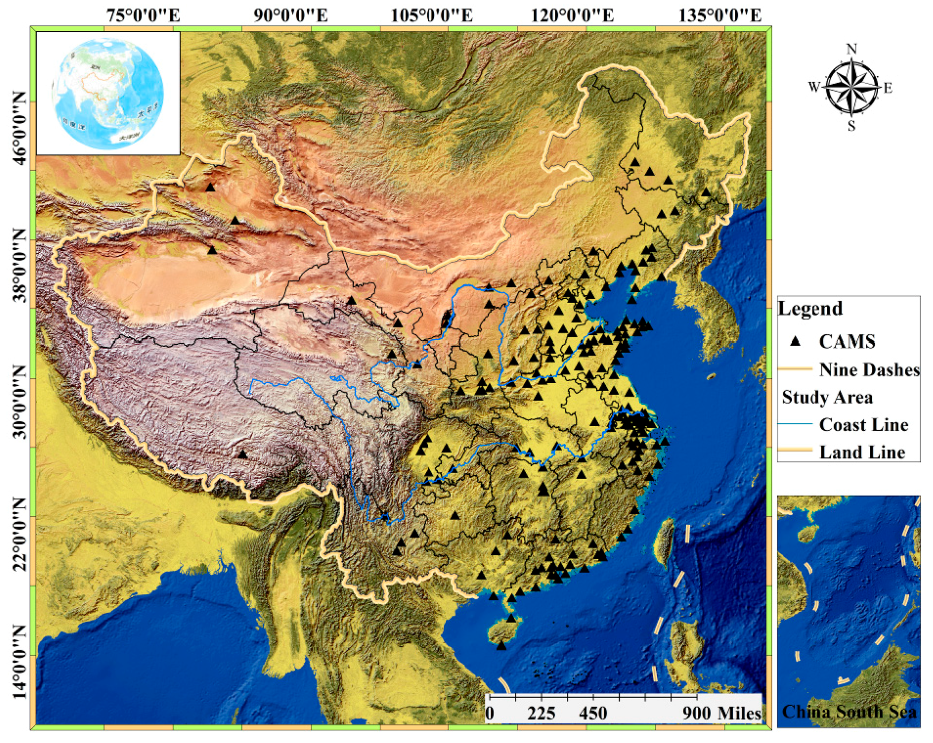
Figure 2.
The monthly dynamics of the principal air pollutants over China (2014 and 2015). Graphs (A–F) represent the monthly concentration of PM2.5 (μg/m−3), PM10 (μg/m−3), CO (mg/m−3), SO2 (μg/m−3), NO2 (μg/m−3), and O3 (μg/m−3) in 2014, respectively; Graphs (G–L) represent the monthly concentration of PM2.5 (μg/m−3), PM10 (μg/m−3), CO (mg/m−3), SO2 (μg/m−3), NO2 (μg/m−3), and O3 (μg/m−3) in 2015, respectively.

Figure 3.
The spatial pattern of the mean concentrations (during January, February, November, and December) of the principal air pollutants over China (2014 and 2015). Graphs (A–F) represent the spatial pattern of PM2.5, PM10, CO, SO2, NO2, and O3 in 2014, respectively; Graphs (G–L) represent the spatial pattern of PM2.5, PM10, CO, SO2, NO2, and O3 in 2015, respectively.
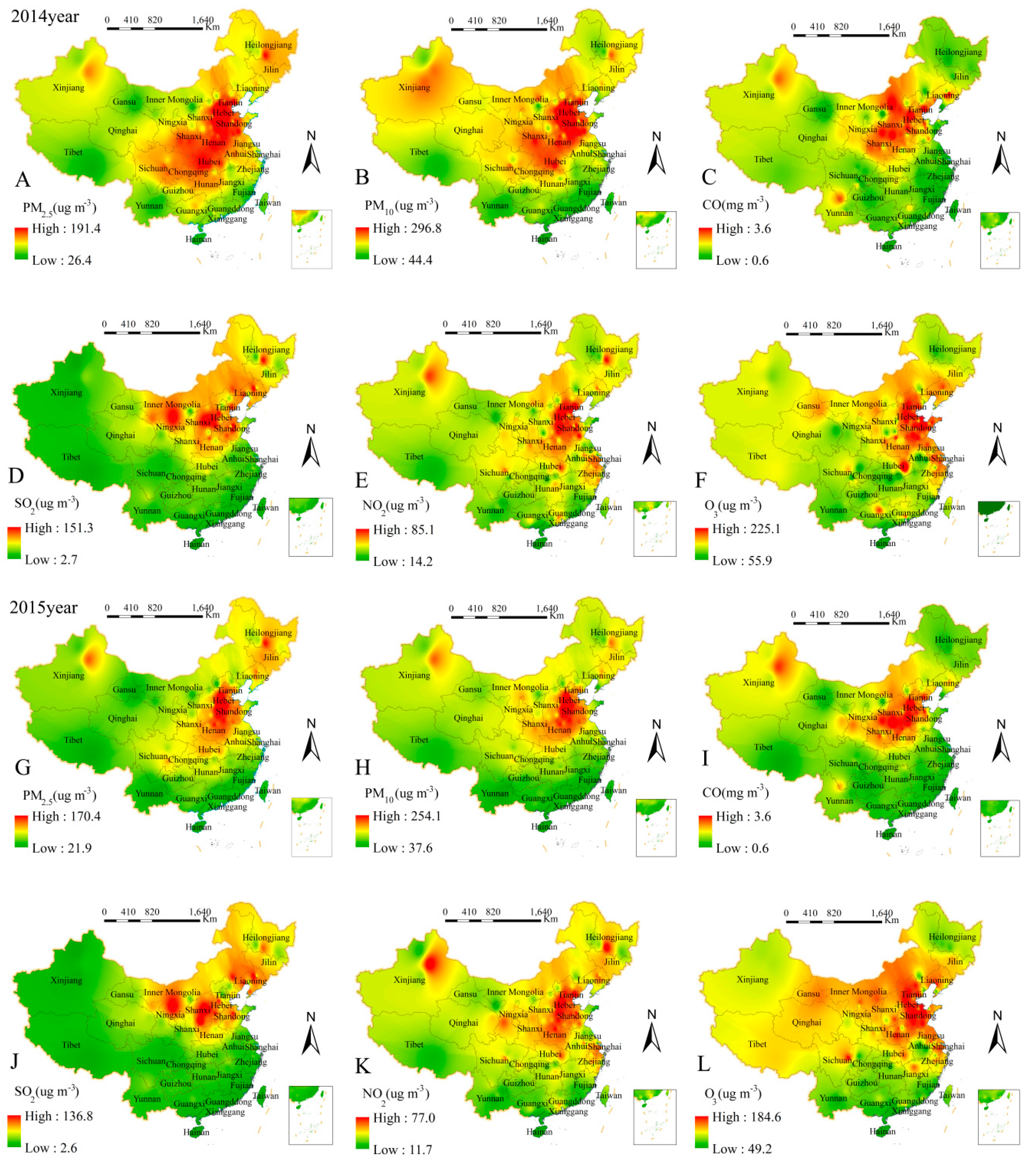
Figure 4.
The daily dynamics of the principal air pollutants in the 17 most polluted cities (2014 and 2015).
Figure 4.
The daily dynamics of the principal air pollutants in the 17 most polluted cities (2014 and 2015).

Figure 5.
The average concentration of the principal air pollutants in Beijing-Tianjin-Hebei during January, February, November, and December (2014 and 2015). Units: PM2.5 (μg/m−3), PM10 (μg/m−3), CO (mg/m−3), SO2 (μg/m−3), NO2 (μg/m−3), and O3 (μg/m−3).
Figure 5.
The average concentration of the principal air pollutants in Beijing-Tianjin-Hebei during January, February, November, and December (2014 and 2015). Units: PM2.5 (μg/m−3), PM10 (μg/m−3), CO (mg/m−3), SO2 (μg/m−3), NO2 (μg/m−3), and O3 (μg/m−3).

Figure 6.
The average concentration of the principal air pollutants in Jinan, Zhengzhou, and Shijiazhuang in autumn (2014 and 2015). Units: PM2.5 (μg/m−3), PM10 (μg/m−3), CO (mg/m−3), SO2 (μg/m−3), NO2 (μg/m−3), and O3 (μg/m−3).
Figure 6.
The average concentration of the principal air pollutants in Jinan, Zhengzhou, and Shijiazhuang in autumn (2014 and 2015). Units: PM2.5 (μg/m−3), PM10 (μg/m−3), CO (mg/m−3), SO2 (μg/m−3), NO2 (μg/m−3), and O3 (μg/m−3).

Figure 7.
The relationships among the principal air pollutants in the 17 most polluted cities (2014). All the numbers and red stars represent the correlation coefficients and significant relationships among the principal air pollutants.
Figure 7.
The relationships among the principal air pollutants in the 17 most polluted cities (2014). All the numbers and red stars represent the correlation coefficients and significant relationships among the principal air pollutants.

Figure 8.
The relationships among the principal air pollutants in the most polluted cities (2015). All the numbers and red stars represent the correlation coefficients and significant relationships among the principal air pollutants.
Figure 8.
The relationships among the principal air pollutants in the most polluted cities (2015). All the numbers and red stars represent the correlation coefficients and significant relationships among the principal air pollutants.

Figure 9.
Predicted changes in the principal air pollutants together with temporal dynamics by generalized additive model (GAM) analysis. Rugplot on the x-axis represents the DOY (day of year), and the light blue belts indicate the credible intervals.
Figure 9.
Predicted changes in the principal air pollutants together with temporal dynamics by generalized additive model (GAM) analysis. Rugplot on the x-axis represents the DOY (day of year), and the light blue belts indicate the credible intervals.

Figure 10.
The mind map for decision-makers.
© 2017 by the authors. Licensee MDPI, Basel, Switzerland. This article is an open access article distributed under the terms and conditions of the Creative Commons Attribution (CC BY) license (http://creativecommons.org/licenses/by/4.0/).
Share and Cite
MDPI and ACS Style
Zhou, T.; Sun, J.; Yu, H. Temporal and Spatial Patterns of China’s Main Air Pollutants: Years 2014 and 2015. Atmosphere 2017, 8, 137. https://doi.org/10.3390/atmos8080137
AMA Style
Zhou T, Sun J, Yu H. Temporal and Spatial Patterns of China’s Main Air Pollutants: Years 2014 and 2015. Atmosphere. 2017; 8(8):137. https://doi.org/10.3390/atmos8080137
Chicago/Turabian StyleZhou, Tiancai, Jian Sun, and Huan Yu. 2017. "Temporal and Spatial Patterns of China’s Main Air Pollutants: Years 2014 and 2015" Atmosphere 8, no. 8: 137. https://doi.org/10.3390/atmos8080137
Note that from the first issue of 2016, this journal uses article numbers instead of page numbers. See further details here.