Seasonal Trends of Formaldehyde and Acetaldehyde in the Megacity of São Paulo


Department of Atmospheric Sciences, Instituto de Astronomia, Geofísica e Ciências Atmosféricas (IAG, Institute of Astronomy, Geophysics, and Atmospheric Sciences), Universidade de São Paulo, Rua do Matão 1226, Cidade Universitária, São Paulo—SP 05508-090, Brazil
*
Author to whom correspondence should be addressed.
Atmosphere 2017, 8(8), 144; https://doi.org/10.3390/atmos8080144
Submission received: 5 June 2017
/
Revised: 1 August 2017
/
Accepted: 3 August 2017
/
Published: 8 August 2017
(This article belongs to the Special Issue Tropospheric Ozone and Its Precursors)
Abstract
:The Metropolitan Area of São Paulo (MASP) is the largest megacity in South America, with 21 million inhabitants and more than 8 million vehicles. Those vehicles run on a complex fuel mix, with ethanol accounting for nearly 50% of all fuel sold. That has made the MASP a unique case study to assess the impact of biofuel use on air quality. Currently, the greatest challenge in terms of improving air quality is controlling the formation of secondary pollutants such as ozone, which represents the main air pollution problem in the MASP. We evaluated the temporal trends in the concentrations of ozone, its precursors (formaldehyde, acetaldehyde, and NO2), CO, and NO, from 2012 to 2016. Formaldehyde and acetaldehyde concentrations were frequently higher in winter than in other seasons, showing the importance of meteorological conditions to the distribution of atmospheric pollutants in the MASP. We found no clear evidence that the recent growth in ethanol consumption in Brazil has affected acetaldehyde concentrations, which are associated with emissions from ethanol combustion. In fact, the formaldehyde/acetaldehyde ratio remained relatively constant over the period studied, despite the change in the fuel consumption profile in the MASP.
1. Introduction
The metropolitan area of São Paulo (MASP), the most important economic region in Brazil, located in São Paulo State, in southeastern Brazil, is one of the largest urban agglomerations in the world. It covers an area of 8051 km2, with 21 million inhabitants, and the urban area is concentrated in ≈2500 km2 [1]. The state of São Paulo is the leading producer of sugarcane/ethanol in Brazil, accounting for 53.4% of sugarcane production (337.7 million tons per crop), 48.4% of ethanol production (13.7 billion liters per crop) and 61.6% of sugar production (21.9 billion tons per crop). Sugarcane cultivation occupies 6.17 million hectares, nearly 25% of the state [2]. The nearest sugar cane plantation and ethanol refinery are ≈150 km from the MASP, the harvest occurring between May and October. The effects of ethanol production on the atmospheric concentrations of volatile organic compounds (VOCs), such as aldehydes and ethanol itself, are still unknown in Brazil, and there are few data in literature. Studies conducted near the city of Ribeirão Preto (320 km from the MASP), a region that produces more than 1.9 billion liters of ethanol a year, reported ethanol concentrations of 3750 ± 430 nmol/L in rainwater [3] and 12.4–14.8 ppbv in the atmosphere [4], compared with only 10 ppbv in the atmosphere over the third largest fuel ethanol refinery in the United States in June–July 2013 [5].
The Official Brazilian National Inventory stated that contributions from land use change, forests, and agribusiness account for more than 50% of atmospheric emissions (expressed as CO2 equivalent), whereas those same sectors account for less than 1% of atmospheric emissions in the MASP [6]. The energy sector is responsible for ≈80% of atmospheric emissions in the MASP, 75% being attributable to the transportation sector (vehicle emissions) [7].
Megacities around the world face environmental problems associated with rapid, unplanned demographic growth, air quality deterioration being one of the most prevalent environmental hazards and responsible for health problems among the population [8]. Vehicle emissions have been recognized as the main air pollution source in the MASP, where there are more than 8 million vehicles burning a mix of fossil fuels and biofuels, accounting for 97% of CO, 76% of hydrocarbons, 68% of nitrogen oxides (NOx), 17% of SOx, and 40% of particulate matter, in 2015 [9]. To minimize this hazardous situation, the Brazilian vehicle emissions control program (PROCONVE), created in the 1980s, has resulted in significant decreases in the concentrations of pollutants in the last decades in the MASP [8,10,11,12]. Nevertheless, the air quality standards are often exceeded, especially that for ozone, which represents one of the main air pollution problems. Ozone, a secondary pollutant produced in the atmosphere by nonlinear interaction among NOx and VOC during photochemical processes, frequently surpasses the attention concentration (200 µg/m3 in 8 h) established by the São Paulo State Environmental Agency—CETESB. In addition, an analysis of the trends in the three-year 8-h moving means in the MASP showed that the maximum ozone concentrations have remained relatively constant over the last 15 years, with no decreasing trend [9]. However, the concentrations of ozone precursors have decreased as a result of PROCONVE [13,14]. Empirical findings and modeling hypotheses suggest that ozone production over the MASP is VOC-limited [15,16]. Ozone isopleth simulations conducted in the MASP have estimated a VOC/NOx ratio of approximately 11 [15]. Those results indicate a VOC-limited atmosphere, in which a 30% reduction in VOC emissions would result in a 30–42% reduction in ozone concentrations.
Fuel consumption and the number of vehicles circulating in the MASP are shown in Figure 1. Vehicles in the MASP fleet run on gasohol (75% gasoline + 25% anhydrous ethanol), hydrous ethanol, or diesel with 8% biodiesel (from soy). Large quantities of ethanol have been consumed in the MASP, where ethanol has accounted for nearly 50% of all fuel sold since 2008, as can be seen in Figure 1. Ethanol is still used in older (pre-2007) vehicles, which are powered exclusively by hydrous ethanol. Since 2003, ethanol has also been used in flex-fuel vehicles, which can run on hydrous ethanol or gasohol and currently account for 40% of the vehicle fleet in the MASP (Figure 1).
Ethanol is well-recognized as a less-polluting vehicle fuel, in terms of local emissions (lower emissions of particulate matter, sulfur, and lead) and emissions of greenhouse gases (carbon dioxide and methane) [18]. However, several studies have implicated ethanol in certain air quality problems [19,20,21,22,23]. Ethanol contributes to ozone formation in two distinct ways: by direct emissions of acetaldehyde resulting from incomplete combustion; and by evaporative emissions. Although ethanol has low reactivity and a low capacity for ozone formation, it is converted to acetaldehyde and peroxyacetyl nitrate by oxidation and photo-oxidation processes in the atmosphere [12]. The reasons for exceedances of the ozone air quality standard in the MASP are not fully understood, although emissions from ethanol combustion might be responsible [8,12]. Previous studies have suggested that ozone in the MASP should have been reduced by the shift from ethanol use to gasohol use by the owners of flex-fuel cars [19,20,21]. Another study showed that, in comparison with gasoline, the use of E85 (gasoline containing 85% ethanol) slightly increases ozone in the presence or absence of fog under summer conditions but increases ozone significantly under winter conditions [23].
The cause of the elevated concentrations of ozone and the role that ethanol use plays in ozone formation in the atmosphere over MASP are still open questions [22,23]. Although the annual mean concentrations of other air pollutants (NOx, CO, and PM10) showed a decreasing trend in the MASP, no trend has been observed for ozone [8,10,11,12,13]. However, increases in ozone concentrations have been observed at some air quality monitoring stations operated by CETESB [9].
In this study, we show seasonal trends in the concentrations of ozone and its key precursors, as well as in those of aldehydes (formaldehyde and acetaldehyde) and NO2, between 2012 and 2016. We provide a detailed analysis of meteorological conditions, analyzing their relationship with ozone, ozone precursors, and other pollutants (NO and CO), in order to further understanding of the photochemical process and of the effect of weather on the regulation of pollutant concentrations in the atmosphere, as well as of the effects of increased ethanol use by vehicles in the MASP.
2. Materials and Methods
2.1. Sampling Site and Study Period
Concentrations of aldehydes, NO, NO2, CO, and ozone were obtained from the CETESB air quality monitoring network [24]. The sampling site was the Pinheiros air quality monitoring station (23°33′39.77″ S, 46°42′6.62″ W), located in the MASP western region, near a busy street and 200 m from one of the busiest roads (Marginal Pinheiros). The analyzer devices and analytical methods employed for those pollutants are summarized in Table 1. Carbonyl samples were collected over a total of 246 days during the 2012–2016 period. Samplings were performed over 24-h periods once every 6 days, on weekdays and weekends. We performed 48 samplings (38 weekday samplings and 10 weekend samplings) in 2012; 35 (28 weekday samplings and 7 weekend samplings) in 2013; 49 (35 weekday samplings and 14 weekend samplings) in 2014; 57 (42 weekday samplings and 15 weekend samplings) in 2015; and 57 (41 weekday samplings and 16 weekend samplings) in 2016.
2.2. Formaldehyde and Acetaldehyde Measurements
The most well-known and well-established method for collecting gas-phase carbonyl compounds is the 2,4-dinitrophenylhydrazine (2,4-DNPH) technique. The sampling and analyses used in the 2,4-DNPH technique follow the standard US EPA TO-11A method [25], and the technique has been largely applied in different places and field campaigns [26,27,28,29,30,31,32,33,34], as well as in previous campaigns carried out in the MASP [35,36,37,38]. It is based on the specific reaction of carbonyl compounds to 2,4-DNPH in the presence of a strong acid, as a catalyst, to form stable color hydrazone derivatives [25], which are then identified by high performance liquid chromatography (HPLC) with ultraviolet detection.
Most of the aldehyde samplings were performed once a week, over a 24-h period, using an automatic pump with a 0.7 L/min flow rate. The samples were collected in commercial silica cartridges coated with 2,4-DNPH solution. To avoid artifacts, a potassium iodide scrubber for ozone retention was used and replaced each day of sampling [39]. After the samples had been collected, the cartridges were duly sealed, packed, and refrigerated until the extraction procedure. In the laboratory, blanks and samples were eluted by acetonitrile with a syringe and transferred to 5-mL volumetric flasks. All solvents and reagents were HPLC grade.
The derived carbonyls were analyzed by HPLC (LC-10A; Shimadzu, Tokyo, Japan). Hydrazones were separated on a Zorbax-ODS column (4.6 mm × 250 mm, 5 µm; Agilent Technologies, Wilmington, DE, USA) with a 365-nm UV detector [40]. Elution was performed with an acetonitrile/water solution (65:35, acetonitrile:water, v/v) as a mobile phase and filtered through a cellulose membrane (0.45 µm pore size). The mobile phase flow rate was 1.0 mL/min, and the injection volume was 10 µL. Carbonyls in the air samples were quantified using the external calibration data from the calibration curve derived from carbonyl-DNPH standards (Sigma-Aldrich, St. Louis, MO, USA). The precision of DNPH method + HPLC technique and their limit of detection are shown in Table 1.
2.3. NO, NO2, CO, and Ozone Measurements
NO, NO2, CO and O3 were measured hourly at the Pinheiros air quality monitoring station [24]. The analytical methods and analyzer devices employed, together with their precision and detection limits, are summarized in Table 1. Calibration procedures for the air quality network were automatically performed by CETESB, on a daily basis, for every instrument at all of the air quality monitoring stations.
2.4. Meteorological Parameters and Ancillary Data
Hourly meteorological data (temperature, precipitation, relative humidity, and incoming solar radiation) were provided by the Meteorological Station of the University of Sao Paulo, Institute of Astronomy, Geophysics, and Atmospheric Sciences [41]. Instruments were calibrated on a regular basis, and data quality control analysis procedures were routinely performed. The station has maintained an important observational database of information collected since 1932. In the present study, seasons were defined in relation to the southern hemisphere, as follows: summer from December to February; autumn from March to May; winter from June to August; and spring from September to November. Fuel consumption data were provided by the Brazilian National Petroleum Agency [17] and the number of vehicles operating in the region was obtained from the mobile source inventory for the São Paulo State [9].
3. Results and Discussion
3.1. Seasonal Variations in Formaldehyde and Acetaldehyde Concentrations
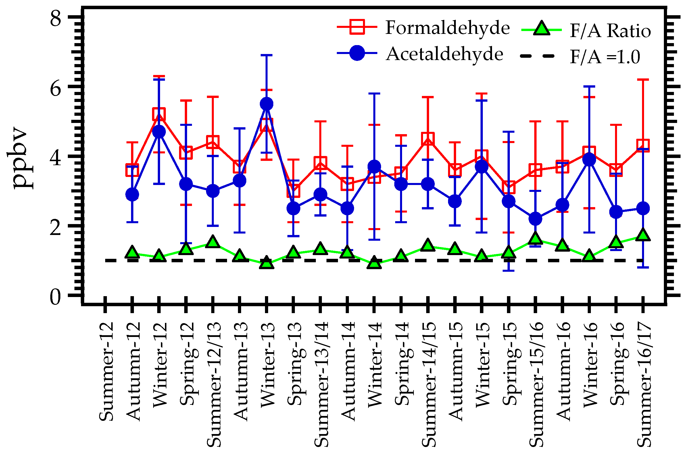
The seasonal variations in the 246 samples of formaldehyde and acetaldehyde, corresponding to 246 days sampled between 2012 and 2016, are shown in Figure 2. Seasonal mean formaldehyde concentrations ranged from 3.0 ± 0.9 ppbv (spring 2013) to 5.2 ± 1.1 ppbv (winter 2012), with a mean of 3.9 ± 1.3 ppbv for the study period as a whole (Figure 2). Formaldehyde was the most abundant carbonyl in 18 of the 20 seasons sampled. The mean acetaldehyde concentration for the study period as a whole was 3.2 ± 1.3 ppbv, ranging from 5.5 ± 1.4 ppbv in the winter of 2013 to 2.2 ± 0.8 ppbv in the summer of 2015/2016.
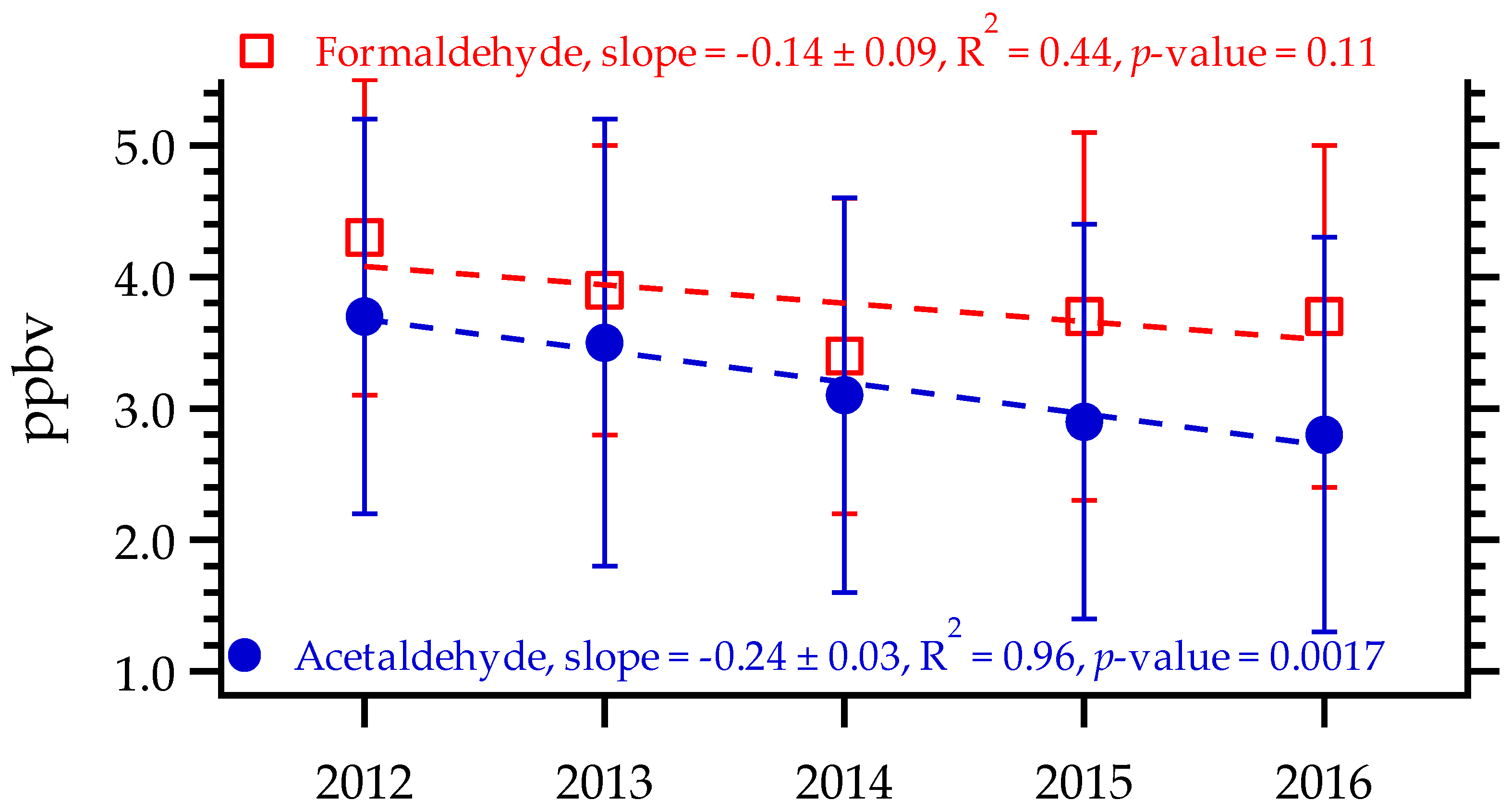
As can be seen in Table 2, the highest annual mean concentrations for formaldehyde and acetaldehyde (4.3 ± 1.2 and 3.7 ± 1.5, respectively) were recorded in 2012, whereas the lowest (3.7 ± 1.3 and 2.8 ± 1.5, respectively) were recorded in 2016. Decreases in the atmospheric concentration of VOCs have recently been observed in the MASP [38,42]. From 2012 to 2016, the observed trend for the mean annual concentrations of formaldehyde was −0.14 ppbv/year (Fcalculated < Fcritical: 2.4 < 10), with no statistical significance (p > 0.05), whereas that for the mean annual concentrations of acetaldehyde (−0.24 ppbv/year; Fcalculated > Fcritical: 72 > 10) was significant (p > 0.0017; Figure 3). The trend toward a slight decrease in the aldehyde concentrations in the MASP runs contrary to the expectation that the increase in ethanol sales in the MASP (Figure 1) would result in higher concentrations of atmospheric acetaldehyde. Some studies have demonstrated that an increase in the quantity of ethanol sold increases evaporative (hot-soak, running loss, resting loss, gas station leak/spill) emissions of ethanol [43]. In the United States, the use of ethanol in gasoline has led to an increase in the ambient concentration of ethanol [44], as well as an increase in acetaldehyde emissions [45]. We believe that evaporative emissions can play a significant role in the formation of ozone, the atmospheric concentration of which cannot be explained by exhaust emissions alone.
The concentrations of atmospheric formaldehyde and acetaldehyde were often higher in winter than in other seasons, in accordance with the meteorological conditions, given that vehicle emissions can be considered constant all over the year. As can be seen in Figure 4, the summer/winter, autumn/winter, and spring/winter carbonyl ratios were lower than 1.0 in most cases, except for the summer/winter and spring/winter formaldehyde ratios in 2014 and the summer/winter formaldehyde ratio in 2015. This pattern was similar to that observed in the city of Londrina, located in the state of Paraná (Table 3), where the concentrations of formaldehyde and acetaldehyde have been found to be higher in winter [29]. However, the pattern observed in the present study differed from those reported in studies conducted in urban areas in China and France [30,31,32,33], where the summer/winter, autumn/winter, and spring/winter ratios were often higher than 1.0 for formaldehyde and acetaldehyde, indicating that their concentrations were lower in winter.
3.2. Seasonal Meteorological, NO, NO2, CO, and Ozone Variations
As discussed in previous studies [10,16,38,42,46], meteorological conditions are key factors in the modulation of pollutant concentrations in the MASP. The region is characterized by a dry season (winter, June to August) and a rainy season (summer, December to March), bracketed by intermediate conditions (in spring and autumn). In general, the minimum daily temperatures and minimum relative humidity occur during July and August, respectively, and the maximum daily temperatures occur in February [47].
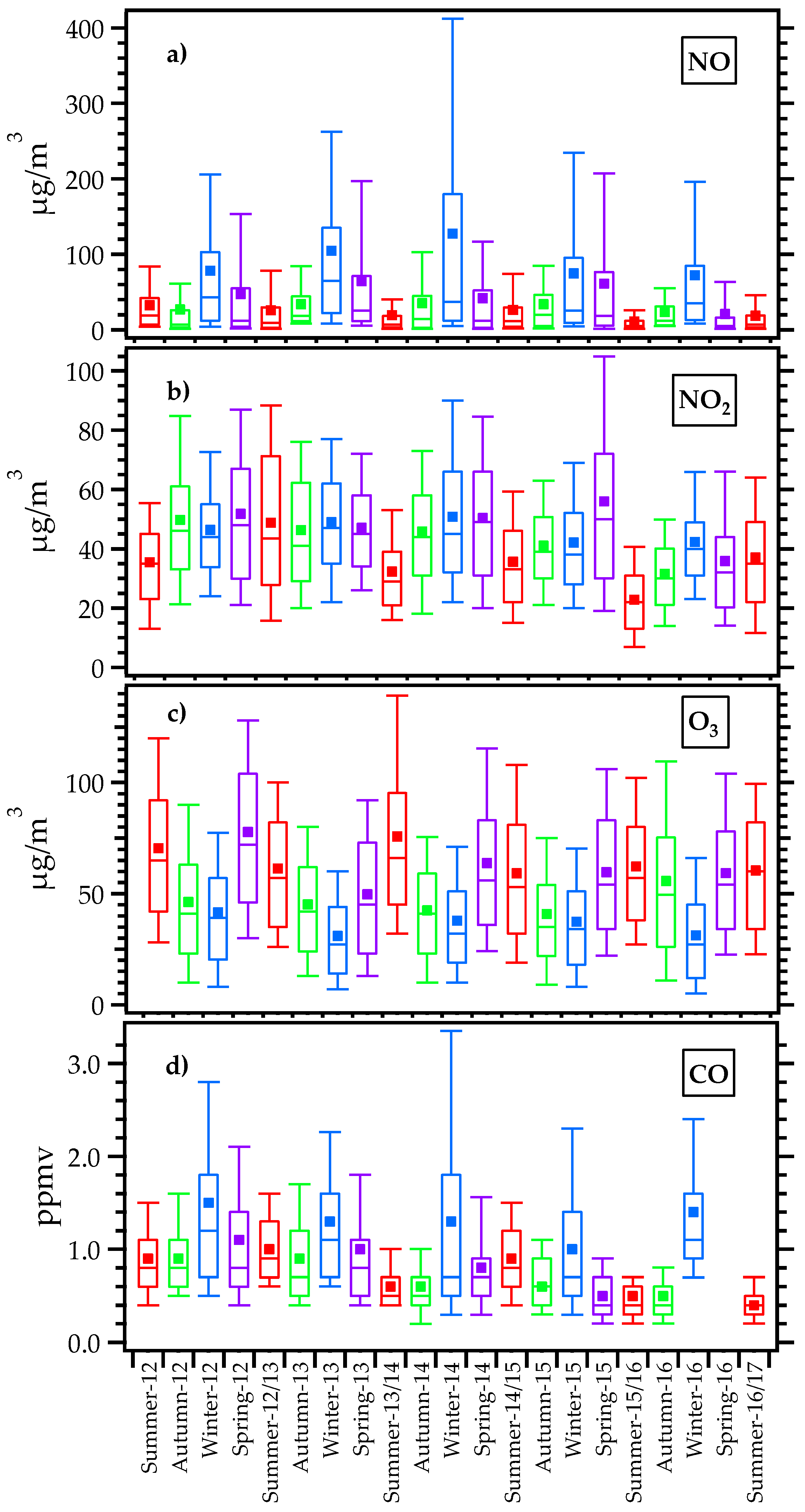
Among the synoptic systems that operate in the MASP, frontal systems and their passage are of chief importance. Whereas heat fronts typically trigger rain events, the passage of cold fronts in winter intensifies the southern quadrant winds, bringing polar air masses and lowering the temperature. Another important synoptic phenomenon in summer in the Brazilian Southeastern region is the South Atlantic Convergence Zone (SACZ), the increased intensity of which causes rainfall events. Meteorological conditions (accumulated rainfall, temperature, and incoming solar radiation) during the period studied are shown, by season, in Figure 5. The main characteristics of winter in the MASP are low solar radiation, temperature, and precipitation, together with 3–5 times more thermal inversions within the planetary boundary layer below 200 m than in other seasons [9]. Consequently, winter has been characterized by the accumulation of primary pollutants such as CO and NO (Figure 6a,d). The winter of 2014 was the driest season, with 101 mm of accumulated rainfall, compared with 859 mm during the rainiest season (summer of 2012/2013). The mean monthly temperature ranged from 14.4 °C in June 2016 to 24.3 °C in February 2014. The mean daily solar radiation, which correlates directly with positive photochemical production, was higher during summer and spring.
The meteorological conditions observed during 2013, 2014, and 2015 were atypical. The driest period in eleven years, with precipitation 13% lower than the climatological mean, occurred in 2014, the driest months being January, February, June, July, September, and October. In addition, throughout 2014, the monthly mean temperatures were higher than the climatological mean, as well as the monthly mean levels of incoming solar radiation, especially in January, when the total maximum radiation set a record—8478 W/m2 (climatological mean, 6970 W/m2)—the highest level since 1961 [48]. In contrast, the precipitation in 2013 was 7% higher than the climatological mean, particularly in summer and winter [49]. A similar pattern was observed in 2015, when precipitation was 30% higher than the climatological mean, mainly during spring, when it was more than twice the respective climatological mean. Nevertheless, the monthly mean temperatures were higher than the respective climatological means throughout the year, making 2015 an extremely wet and warm year [48]. However, although ethanol was the best-selling fuel, with ethanol sales reaching 9 × 10⁶ m3 in that year (Figure 1), no significant peaks were observed in the concentrations of aldehydes (Figure 2) or ozone (Figure 6c).
The seasonal variability of NO and NO2 concentrations is presented in Figure 6a,b, respectively. Higher concentrations of NO were observed in winter periods, the mean being highest (127 µg/m3) in the winter of 2014 and lowest (11 µg/m3) in the summer of 2015/2016. Except in the summer of 2012/2013, the mean NO2 concentrations were lowest in the summer periods, whereas they were highest in the winter and spring periods. The seasonal mean NO2 concentration was also lowest (23 µg/m3) in the summer of 2015/2016, whereas it was highest (52 µg/m3) in the spring of 2012. During the study period as a whole, the maximum NO2 concentration was 250 µg/m3, which did not exceed the 1-h air quality standard for the state of São Paulo (260 µg/m3) [9].
The seasonality of ozone concentrations is presented in Figure 6c. The seasonal mean was calculated using the daily 8-h mean (from 11 a.m. to 6 p.m.). The data show marked seasonality. Because ozone is formed in the atmosphere by photochemical reactions that are dependent on factors such as solar radiation and temperature (Figure 5), the spring and summer were the seasons that were most favorable to ozone formation (Figure 6c). The seasonal mean ozone concentration was highest (78 µg/m3) in the spring of 2012 and lowest (31 µg/m3) in the winter of 2016. Higher mean ozone values were frequently observed during the spring. The incidence of solar radiation can be higher in summer (Figure 5). However, in the MASP, summer is characterized by a lower number of days with clear sky conditions in the afternoon due to rain events or sea breeze circulation bringing humidity and cloudiness (Figure 5), which can reduce ozone formation by photochemical reactions [10]. During the study period, the highest 8-h mean ozone concentration recorded at the Pinheiros station was 265 µg/m3 in 2014, a year in which the ozone standard (140 µg/m3 in 8 h) was reportedly exceeded on 35 days.
The seasonality of CO concentrations is shown in Figure 6d, with the maximum mean value reported as 7.3 ppmv. Therefore, no exceedances of the CO standard (9 ppmv in 8 h) were observed during the study period at the Pinheiros air quality monitoring station. As previously mentioned, the mean concentrations of atmospheric pollutants in the MASP are higher during the colder seasons, when there is a prevalence of thermal inversions near the surface, weak winds, and lower precipitation (Figure 5), causing pollutants to accumulate. The seasonal mean CO concentration was highest (1.5 ppmv) in the winter of 2012 and lowest (0.4 ppmv) in the summer of 2016/2017. This marked trend in seasonal CO concentrations has also been observed in other studies of air quality in the MASP [10,50].
Some studies have indicated that the formaldehyde production from isoprene oxidation is dependent on the NOx concentration and temperature [51]. In the present study, NOx reached maximum values of 400 ppbv, with a mean of ≈50 ppbv, at the Pinheiros air quality monitoring station, between 2012 and 2016. In the MASP, near a small urban park (≈5 km from Pinheiros station), analyses of 2998 hourly hydrocarbons samples performed in 2013, equally distributed across all seasons, showed a maximum isoprene concentration of 3.9 ppbv, with a mean value of 0.38 ± 0.47 ppbv [42]. Another study, in which measurements were taken from 8 February to 23 April, 2013 [52], reported mean isoprene and acetaldehyde concentrations of 1.06 ± 0.68 ppbv and 3.42 ± 1.98 ppbv, respectively, near an avenue with heavy vehicular traffic. Whereas the contribution of isoprene from vehicle emissions has been reported for other cities worldwide [53,54,55], studies in the MASP briefly discussed isoprene sources [42,52]. The study conducted in the MASP shows that even compounds associated with biogenic or secondary sources, such as acetone, acetaldehyde and MVK + MACR, presented a high nighttime correlation with CO (R2 > 0.8) [52]. High nighttime correlation indicates that VOCs share a common source with CO, for instance combustion, instead evaporation [52]. Moreover, the atmospheric concentrations are affected by meteorological conditions, especially during nighttime due to the lower boundary layer and calm winds contributing to the increase of atmospheric pollutants concentrations [56,57]. Therefore, both vehicular emissions and biogenic emissions should be considered in the MASP. The presence and emission of isoprene from biogenic sources in urban areas cannot be ignored [54,56,57] and the contribution of biogenic sources and their role in formaldehyde formation need to be thoroughly addressed in future studies in the MASP.
3.3. F/A Ratio
It is known that formaldehyde and acetaldehyde are emitted as primary pollutants by vehicle fleets in urban centers [38,58] and by biogenic sources (emissions from trees) [59,60]. In addition, they are important secondary pollutants created through oxidation reactions of hydrocarbons from anthropogenic or biogenic emissions [61,62]. However, these carbonyls (formaldehyde and acetaldehyde) are removed by photochemical reactions, contributing to the production of ozone, as well as of the OH and HO2 radicals [61,63]. The atmospheric concentrations of formaldehyde and acetaldehyde are the result of these different processes of emission, production, and photochemical consumption, as is the F/A ratio [64,65,66,67]. The photolysis of carbonyls and their chemical reactions with the OH radical are the dominant processes in the removal of carbonyls from the atmosphere, changing the F/A ratio by altering the distribution of atmospheric formaldehyde and acetaldehyde [64,65,66,67]. Therefore, the F/A ratios should be higher in the presence of high hydrocarbon concentrations and photochemical conditions that are more intense.
The mean seasonal F/A ratios, ranging from 0.9 in winter to 1.7 in summer, are shown in Figure 2. Table 2 shows F/A ratios, yearly, revealing no trend. During the period studied, the mean F/A ratio in the MASP was higher (1.3–1.7), which implied intense photochemical reactivity leading to the formation of atmospheric carbonyls in summer. This high photochemical reactivity corresponds to the high levels of incoming solar radiation in summer and spring (Figure 5). The mean F/A ratio was lower (0.9–1.1) in winter, due to lower incoming solar radiation (Figure 5) and possible accumulation of acetaldehyde during thermal inversions.
Several studies conducted in urban areas of Brazil have reported F/A ratios below 1.0 [27,28,29,68]. The high acetaldehyde concentration in Brazil has been attributed to vehicle emissions and to the composition of the biofuels used. Incomplete combustion of ethanol results in higher acetaldehyde emissions, whether the vehicle is powered by hydrous ethanol or gasohol. For instance, there is evidence that the addition of ethanol to gasoline results in a substantial (100–200%) increase in acetaldehyde emissions [69]. However, previous studies conducted in the MASP [38,68] have shown that, over the last 30 years, there has been a reduction in acetaldehyde emissions from light-duty vehicles, resulting in higher F/A ratios. During the 1980s, the F/A ratio in the MASP was frequently below 0.5 [26], whereas it is currently above 1.0. As discussed in a previous study [38], despite a considerable increase in ethanol sales in the MASP, attributable in part to an increase in the number of light-duty flex-fuel vehicles (Figure 1), there is no evidence of an increase in acetaldehyde concentrations, as would be reflected in the F/A ratio. The technological improvements incorporated into the design of the flex-fuel vehicles prevented any significant increase in aldehyde concentrations in the atmosphere [38].
Some studies have demonstrated an increase in acetaldehyde emissions associated with biodiesel use [27,70]. A study conducted in the city of Salvador, Brazil, showed that the addition of 5% biodiesel to diesel fuel resulted in an increase in acetaldehyde emissions and a consequent change in the atmospheric F/A ratio [27]. However, in the present study, we found that the F/A ratio was not sensitive to the recent increase in biodiesel consumption in the MASP (data not shown).
3.4. Primary vs Secondary Sources of Aldehydes in the MASP
Pearson’s correlation coefficient was used in order to investigate the characteristics of sources and sinks or interactions among the compounds analyzed in the MASP. Table 4 shows the correlation coefficients for formaldehyde, acetaldehyde, and other pollutants measured in this study, in summer and winter, from 2012 to 2016. In both seasons, good correlations were observed between formaldehyde and acetaldehyde (R > 0.9), suggesting that both carbonyls came from the same source and had common sinks in both seasons. Both aldehydes showed stronger correlations with primary vehicular pollutants during winter. CO is well-known as primary pollutant, mainly from light-duty vehicle emissions resulting from incomplete combustion, whereas NO is known as a primary pollutant produced mainly by diesel-powered heavy-duty vehicles [14,31,71]. Acetaldehyde correlated better with CO and NO in winter (R = 0.85 and 0.79, respectively) than in summer (R = 0.61 and 0.55, respectively). Formaldehyde also correlated better with CO and NO in winter (R = 0.70 and 0.59, respectively) than in summer (R = 0.42 and 0.38, respectively). However, formaldehyde and acetaldehyde both showed weaker correlations with ozone in winter (R = 0.46 and 0.33, respectively) than in summer (R = 0.65 and 0.57, respectively). This suggests that primary emissions from vehicles, rather than photochemical processes, were the major sources of aldehydes in winter, whereas in summer they arise as primary pollutants from vehicle emissions and as secondary pollutants from photochemical processes. It is of note that formaldehyde showed a stronger correlation with ozone, whereas acetaldehyde presented stronger correlations with primary pollutants, in both seasons. These findings are in alignment with our finding that the mean F/A ratio was higher in summer (1.5 ± 0.2) than in winter (1.0 ± 0.1), indicating that secondary sources make a significant contribution to formaldehyde concentrations in summer. Better correlations between formaldehyde and ozone in summer than in winter have also been reported in studies conducted in other urban areas, such as those conducted in Rome [72] and in Hong Kong [31].
3.5. OH Reactivity and Ozone Formation
In urban atmospheres, the photochemical reactions leading to the formation of tropospheric ozone, as well as of the OH, HO2, and organic peroxy radicals, are mainly related to the concentration and reactivity of ozone precursors, especially VOCs. Aldehydes are important precursors of ozone, and each species has an inherent reactivity, predominantly related to the reactions with the OH radical and the potential to produce ozone [73,74,75]. To estimate potential formation reactions, reactivity scales have been used extensively in various studies conducted in Brazil, showing the impact that individual compounds have on ozone formation [15,19,37,38,42,68,76]. Two methods in particular have been employed: the maximum incremental reactivity (MIR) coefficient [73]; and the propylene equivalent (propy-equiv) scale.
MIR coefficients represent the ozone formation potential (OFP), defined as the ozone mass produced per gram of VOC added into the system. The MIR value, which is dimensionless, has been estimated for a large quantity of compounds [74] with the following equation:
in which ci is the concentration of the organic compound i, in µg/m3, and MIR is the coefficient for the individual compound i.
OFP (µg/m3) = ci × MIRi
The propy-equiv scale is an OH-reactivity indicator based on a scale normalized to the reactivity of propylene (kOH = 26.3 × 10⁻¹² cm3/molecule × s) and indicates the concentration of propylene required to produce a carbon oxidation rate equal to that of a specific VOC species [77]:
in which ci is the concentration of the compound i, kOHi is the reactivity rate of the compound i, and kOH (C2H6) is the reactivity rate of propylene. The propy-equiv scale was used in order to analyze the importance of the various VOC species in producing ozone at a specific location [77].
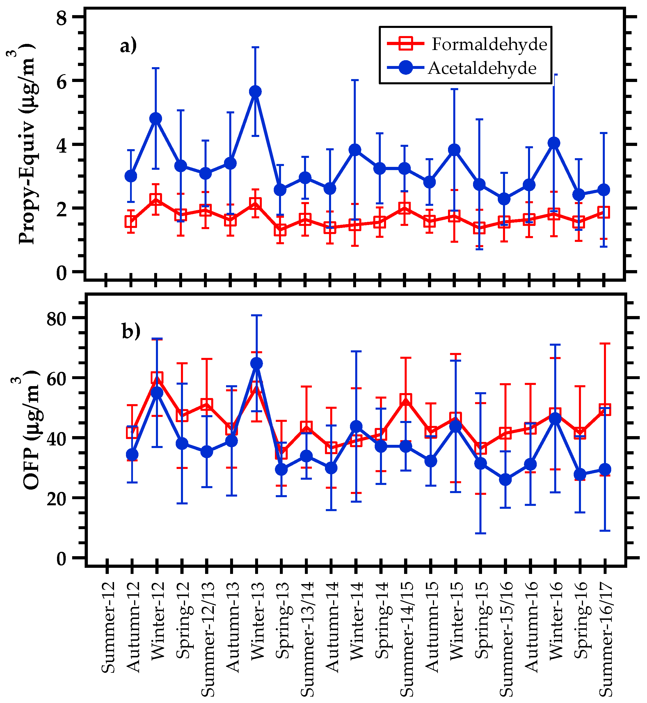
The OFP and propy-equiv scale values for acetaldehyde and formaldehyde concentrations are shown in Figure 7. In the present study, acetaldehyde contributed much more to propy-equiv concentrations than did formaldehyde, due to the differences in their reactivity rates (15 and 9.37 × 10⁻¹² cm3/molecule × s, respectively) [73]. In terms of seasonality, higher contributions (up to 7 µg/m3) were observed during winter, when higher concentrations of acetaldehyde were also observed. This pattern differs from those observed in cities in China, where propy-equiv values have been found to be higher in summer [30,32]. For example, despite differences in seasonality, the maximum values observed in the Chinese city of Nanning were similar to those observed in the MASP (6.0–9.9 µg/m3) [30].
In the present study, the OFPs for acetaldehyde and formaldehyde ranged from 26 to 65 µg/m3 and from 35 to 60 µg/m3, respectively. Despite the maximum values observed, the mean OFP was higher for formaldehyde than for acetaldehyde (45 µg/m3 vs. 37 µg/m3). Higher OFP were frequently observed in summer, when photochemical reactions were also favored by solar radiation availability leading to ozone formation. In the MASP, the mean seasonal OFP was highest in winter (50 µg/m3) and summer (48 µg/m3) for formaldehyde, whereas it was highest in winter for acetaldehyde (51 µg/m3). Although the OFPs were lower than those observed in other megacities [30,32], there is no clear seasonality pattern for the OFPs in the MASP. That could be explained by the effects that meteorological conditions have on pollutant dispersion, as well as by the unfavorable photochemical reactions during wintertime.
4. Conclusions
In this study, we monitored carbonyl compounds in the MASP, evaluating a total of 246 samples collected over a five-year period (2012–2016). The seasonal evaluations showed that concentrations of formaldehyde and acetaldehyde were frequently higher in winter than in other seasons. Seasonal aldehyde ratios showed a pattern different from that observed in other regions around the world, although similar to those reported for other Brazilian cities.
Our results underscore the effect that meteorological conditions have on pollutant concentrations in the MASP atmosphere, with carbonyl concentrations being higher in winter. This pattern was in alignment with those of other pollutants such as CO and NO (both primary pollutants emitted mainly by vehicles) because during the colder months, thermal inversions near the surface prevail, inducing stable atmospheric conditions, weak winds, and less precipitation.
The ozone pattern is related to photochemical activity. Ozone is one of the main pollutants in the MASP, where ozone concentrations often exceed the air quality standard of São Paulo State. During the period under study, exceedances of the ozone standard were observed on 128 days at the Pinheiros station.
During winter, aldehydes correlated better with primary vehicular pollutants and poorer with ozone. In contrast, aldehydes correlated better with ozone in summer, when there are apparently two major sources and sinks of formaldehyde and acetaldehyde: primary emissions and secondary pollutants. This suggests that primary vehicular emissions, rather than photochemical processes, are the major source of aldehydes in the winter. However, the contribution from biogenic sources and their role in formaldehyde formation through secondary process in the MASP should be investigated in future studies.
The propy-equiv and OFP showed higher values in winter. Nevertheless, ozone concentrations were higher during spring, when radiation, temperature, and meteorological conditions were favorable for ozone formation.
Finally, our findings show that the increases in ethanol consumption did not have a direct impact on acetaldehyde concentrations associated with emissions from ethanol combustion, a pattern that seems to have been maintained over the last few years. In addition, evaporative emissions, also associated with the quantity of ethanol sold and contributing to acetaldehyde formation through ethanol reactions in the atmosphere, seemed to have no effect on atmospheric concentrations of acetaldehyde. Furthermore, despite the greater biodiesel content in diesel fuel since 2008, no increases in atmospheric acetaldehyde concentrations were detected. Moreover, the F/A ratio was not sensitive to the changes in the vehicle fuel consumption profile in the MASP. The implementation of programs to control vehicle emissions has resulted in a decrease in the exhaust emissions of primary pollutants such as NO, CO, and VOCs, as evidenced by the lower concentrations of formaldehyde and acetaldehyde.
Acknowledgments
The authors gratefully acknowledge the financial support from the Fundação de Amparo à Pesquisa do Estado de São Paulo (FAPESP, São Paulo Research Foundation), the Brazilian Conselho Nacional de Desenvolvimento Científico e Tecnológico (CNPq, National Council for Scientific and Technological Development), and the Brazilian Coordenação de Aperfeiçoamento de Pessoal de Nível Superior (CAPES, Office for the Advancement of Higher Education). Thiago Nogueira, who is the recipient of grants from the Brazilian Programa Nacional de Pós-Doutorado (PNPD, National Postdoctoral Program) and CAPES, and Pamela A. Dominutti, who was the recipient of a grant from CNPq, both acknowledge the Postgraduate Program in Meteorology at the University of São Paulo Instituto de Astronomia, Geofísica e Ciências Atmosféricas (IAG, Institute of Astronomy, Geophysics, and Atmospheric Sciences) for providing fellowship grants. We are also grateful to the São Paulo State Environmental Agency—CETESB (www.cetesb.sp.gov.br) and the Brazilian Agência Nacional do Petróleo (ANP, National Petroleum Agency; www.anp.gov.br) for allowing access to their data, as well to the IAG Meteorological Station (www.estacao.iag.usp.br) for the meteorological data provided.
Author Contributions
The article was conceived by Thiago Nogueira. Pamela A. Dominutti and Thiago Nogueira defined the location of the data collection sites and downloaded the data, analyzed and interpreted the results. Adalgiza Fornaro and Maria de Fatima Andrade supervised the work and contributed to the interpretation of results. The paper was written by Thiago Nogueira and Pamela A. Dominutti and revised by Adalgiza Fornaro and Maria de Fatima Andrade.
Conflicts of Interest
The authors declare no conflict of interest.
References
- Instituto Brasileiro de Geografia e Estatística (IBGE); Brazilian Institute of Geography and Statistics. Available online: http://cod.ibge.gov.br/QHF (accessed on 25 May 2017).
- União da Indústria da Cana de Açúcar (UNICA). Available online: http://www.unicadata.com.br (accessed on 7 July 2017).
- Felix, J.D.; Willey, J.D.; Thomas, R.K.; Mullaugh, K.M.; Avery, G.B.; Kieber, R.J.; Mead, R.N.; Helms, J.; Giubbina, F.F.; Campos, M.L.A.M.; et al. Removal of atmospheric ethanol by wet deposition. Glob. Biogeochem. Cycles 2017, 31, 348–356. [Google Scholar] [CrossRef]
- Giubbina, F.F.; Scaramboni, C.; de Martinis, B.S.; Godoy-Silva, D.; Nogueira, R.F.P.; Campos, M.L.A.M. A simple method for simultaneous determination of acetaldehyde, acetone, methanol, and ethanol in the atmosphere and natural waters. Anal. Methods 2017, 9, 2915–2922. [Google Scholar] [CrossRef]
- De Gouw, J.A.; McKeen, S.A.; Aikin, K.C.; Brock, C.A.; Brown, S.S.; Gilman, J.B.; Graus, M.; Hanisco, T.; Holloway, J.S.; Kaiser, J.; et al. Airborne measurements of the atmospheric emissions from a fuel ethanol refinery. J. Geophys. Res. Atmos. 2015, 120, 4385–4397. [Google Scholar] [CrossRef]
- MCTI Estimativas Anuais de Emissões de Gases de Efeito Estufa no Brasil. 2016. Available online: http://sirene.mcti.gov.br/documents/1686653/1706227/LIVRO_MCTIC_EstimativaDeGases_Publica%C3%A7%C3%A3o_210x297mm_FINAL_WEB.pdf/61e78a4d-5ebe-49cd-bd16-4ebca30ad6cd (accessed on 7 July 2017).
- Instituto Ekos Brasil. Inventário de Emissões e Remoções Antrópicas de Gases de Efeito Estufa do Município de São Paulo de 2003 a 2009 com atualização para 2010 e 2011 Nos Setores Energia e Resíduos. Available online: http://www.prefeitura.sp.gov.br/cidade/secretarias/upload/meio_ambiente/arquiv (accessed on 7 July 2017).
- Kumar, P.; Andrade, M.F.; Ynoue, R.Y.; Fornaro, A.; de Freitas, E.D.; Martins, J.; Martins, L.D.; Albuquerque, T.; Zhang, Y.; Morawska, L. New directions: From biofuels to wood stoves: The modern and ancient air quality challenges in the megacity of São Paulo. Atmos. Environ. 2016, 140, 364–369. [Google Scholar] [CrossRef] [Green Version]
- CETESB Qualidade do ar no Estado de São Paulo—2016. São Paulo, 2017. Available online: http://ar.cetesb.sp.gov.br/publicacoes-relatorios/ (accessed on 2 May 2017).
- Carvalho, V.S.B.; Freitas, E.D.; Martins, L.D.; Martins, J.A.; Mazzoli, C.R.; Andrade, M.F. Air quality status and trends over the Metropolitan Area of Sao Paulo, Brazil as a result of emission control policies. Environ. Sci. Policy 2015, 47, 68–79. [Google Scholar] [CrossRef]
- Pérez-Martínez, P.J.; Andrade, M.F.; Miranda, R.M. Traffic-related air quality trends in São Paulo, Brazil. J. Geophys. Res. Atmos. 2015, 120, 6290–6304. [Google Scholar] [CrossRef]
- Andrade, M.F.; Kumar, P.; Freitas, E.D.; Ynoue, R.Y.; Martins, J.; Martins, L.D.; Nogueira, T.; Perez-Martinez, P.; Miranda, R.M.; Albuquerque, T.; et al. Air quality in the megacity of São Paulo: Evolution over the last 30 years and future perspectives. Atmos. Environ. 2017, 159, 66–82. [Google Scholar] [CrossRef]
- Nogueira, T.; de Sales Cordeiro, D.; Muñoz, R.A.A.; Fornaro, A.; Miguel, A.H.; Andrade, M.F. Bioethanol and Biodiesel as Vehicular Fuels in Brazil—Assessment of Atmospheric Impacts from the Long Period of Biofuels Use. In Biofuels—Status Perspect; InTech: Rijeka, Croatia, 2015. [Google Scholar] [CrossRef]
- Pérez-Martínez, P.J.; Miranda, R.M.; Nogueira, T.; Guardani, M.L.; Fornaro, A.; Ynoue, R.; Andrade, M.F. Emission factors of air pollutants from vehicles measured inside road tunnels in São Paulo: Case study comparison. Int. J. Environ. Sci. Technol. 2014, 11, 2155–2168. [Google Scholar] [CrossRef]
- Orlando, J.P.; Alvim, D.S.; Yamazaki, A.; Corrêa, S.M.; Gatti, L.V. Ozone precursors for the São Paulo Metropolitan Area. Sci. Total Environ. 2010, 408, 1612–1620. [Google Scholar] [CrossRef] [PubMed]
- Sánchez-Ccoyllo, O.R.; Ynoue, R.Y.; Martins, L.D.; Andrade, M.F. Impacts of ozone precursor limitation and meteorological variables on ozone concentration in São Paulo, Brazil. Atmos. Environ. 2006, 40, 552–562. [Google Scholar] [CrossRef]
- ANP Agência Nacional de Petróleo, Gás Natural e Biocombustíveis. National Agency for Oil, Natural Gas, and Biofuels. Available online: http://www.anp.gov.br (accessed on 1 May 2017).
- Goldemberg, J. Ethanol for a Sustainable Energy Future. Science 2007, 315, 808–810. [Google Scholar] [CrossRef] [PubMed]
- Martins, L.D.; Andrade, M.F. Ozone Formation Potentials of Volatile Organic Compounds and Ozone Sensitivity to Their Emission in the Megacity of São Paulo, Brazil. Water Air Soil Pollut. 2008, 195, 201–213. [Google Scholar] [CrossRef]
- Salvo, A.; Geiger, F.M. Reduction in local ozone levels in urban São Paulo due to a shift from ethanol to gasoline use. Nat. Geosci. 2014, 7, 450–458. [Google Scholar] [CrossRef]
- Madronich, S. Atmospheric chemistry: Ethanol and ozone. Nat. Geosci. 2014, 7, 395–397. [Google Scholar] [CrossRef]
- Jacobson, M.Z. Effects of ethanol (E85) versus gasoline vehicles on cancer and mortality in the United States. Environ. Sci. Technol. 2007, 41, 4150–4157. [Google Scholar] [CrossRef] [PubMed]
- Ginnebaugh, D.L.; Jacobson, M.Z. Examining the impacts of ethanol (E85) versus gasoline photochemical production of smog in a fog using near-explicit gas- and aqueous-chemistry mechanisms. Environ. Res. Lett. 2012, 7, 45901. [Google Scholar] [CrossRef]
- CETESB-QUALAR São Paulo State Environmental Agency (CETESB). Available online: http://www.cetesb.sp.gov.br (accessed on 2 May 2017).
- Environmental Protection Agency (EPA). Method TO-11A Determination of Formaldehyde in Ambient Air Using Adsorbent Cartridge Followed by High Performance Liquid Chromatography. In Compendium of Methods for the Determination of Toxic Organic Compounds in Ambient Air, 2nd ed.; U.S. Environmental Protection Agency: Cincinnati, OH, USA, 1999. [Google Scholar]
- Grosjean, D.; Miguel, A.H.; Tavares, T.M. Urban air pollution in Brazil: Acetaldehyde and other carbonyls. Atmos. Environ. B Urban Atmos. 1990, 24, 101–106. [Google Scholar] [CrossRef]
- Rodrigues, M.C.; Guarieiro, L.L.N.; Cardoso, M.P.; Souza, L.; Gisele, O.; Andrade, J.B.; Carvalho, L.S.; da Rocha, G.O.; de Andrade, J.B. Acetaldehyde and formaldehyde concentrations from sites impacted by heavy-duty diesel vehicles and their correlation with the fuel composition: Diesel and diesel/biodiesel blends. Fuel 2012, 92, 258–263. [Google Scholar] [CrossRef]
- Corrêa, S.M.; Martins, E.M.; Arbilla, G. Formaldehyde and acetaldehyde in a high traffic street of Rio de Janeiro, Brazil. Atmos. Environ. 2003, 37, 23–29. [Google Scholar] [CrossRef]
- Pinto, J.P.; Solci, M.C. Comparison of rural and urban atmospheric aldehydes in Londrina, Brazil. J. Braz. Chem. Soc. 2007, 18, 928–936. [Google Scholar] [CrossRef]
- Guo, S.; Chen, M.; Tan, J. Seasonal and diurnal characteristics of atmospheric carbonyls in Nanning, China. Atmos. Res. 2016, 169, 46–53. [Google Scholar] [CrossRef]
- Cheng, Y.; Lee, S.C.; Huang, Y.; Ho, K.F.; Ho, S.S.H.; Yau, P.S.; Louie, P.K.K.; Zhang, R.J. Diurnal and seasonal trends of carbonyl compounds in roadside, urban, and suburban environment of Hong Kong. Atmos. Environ. 2014, 89, 43–51. [Google Scholar] [CrossRef]
- Lü, H.; Cai, Q.Y.; Wen, S.; Chi, Y.; Guo, S.; Sheng, G.; Fu, J. Seasonal and diurnal variations of carbonyl compounds in the urban atmosphere of Guangzhou, China. Sci. Total Environ. 2010, 408, 3523–3529. [Google Scholar] [CrossRef] [PubMed]
- Jiang, Z.; Grosselin, B.; Daële, V.; Mellouki, A.; Mu, Y. Seasonal, diurnal and nocturnal variations of carbonyl compounds in the semi-urban environment of Orléans, France. J. Environ. Sci. 2016, 40, 84–91. [Google Scholar] [CrossRef] [PubMed]
- Martins, L.D.; Andrade, M.F.; Ynoue, R.Y.; Albuquerque, E.L.; Tomaz, E.; Vasconcellos, P.C. Ambiental volatile organic compounds in the megacity of Sao Paulo. Quim. Nova 2008, 31, 2009–2013. [Google Scholar] [CrossRef]
- Montero, L.; Vasconcellos, P.C.; Souza, S.R.; Pires, M.A.F.; Sánchez-Ccoyllo, O.R.; Andrade, M.F.; Carvalho, L.R.F. Measurements of Atmospheric Carboxylic Acids and Carbonyl Compounds in São Paulo City, Brazil. Environ. Sci. Technol. 2001, 35, 3071–3081. [Google Scholar] [CrossRef] [PubMed]
- Vasconcellos, P.C.; Carvalho, L.R.F.; Pool, C.S. Volatile organic compounds inside urban tunnels of São Paulo City, Brazil. J. Braz. Chem. Soc. 2005, 16, 1210–1216. [Google Scholar] [CrossRef]
- Alvim, D.S.; Gatti, L.V.; dos Santos, M.H.; Yamazaki, A. Estudos dos compostos orgânicos voláteis precursores de ozônio na cidade de São Paulo. Eng. Sanit. Ambient. 2011, 16, 189–196. [Google Scholar] [CrossRef]
- Nogueira, T.; Dominutti, P.A.; Carvalho, L.R.F.; Fornaro, A.; Andrade, M.F. Formaldehyde and acetaldehyde measurements in urban atmosphere impacted by the use of ethanol biofuel: Metropolitan Area of Sao Paulo (MASP), 2012–2013. Fuel 2014, 134, 505–513. [Google Scholar] [CrossRef] [Green Version]
- Pires, M.; Carvalho, L.R.F. An artifact in air carbonyls sampling using C18 DNPH-coated cartridge. Anal. Chim. Acta 1998, 367, 223–231. [Google Scholar] [CrossRef]
- CETESB Concentrações de Formaldeído e Acetaldeído na Atmosfera. Estaçâo Pinheiros, São Paulo-SP (2012–2013). 2015; Volume 1. Available online: http://ar.cetesb.sp.gov.br/publicacoes-relatorios/ (accessed on 2 May 2017).
- IAG Weather Station Bulletin. Available online: http://www.estacao.iag.usp.br (accessed on 2 May 2017).
- Dominutti, P.A.; Nogueira, T.; Borbon, A.; Andrade, M.F.; Fornaro, A. One-year of NMHCs Hourly Observations in São Paulo Megacity: Meteorological and Traffic Emissions Effects in a Large Ethanol Burning Context. Atmos. Environ. 2016, 142, 371–382. [Google Scholar] [CrossRef]
- Gentner, D.R.; Harley, R.A.; Miller, A.M.; Goldstein, A.H. Diurnal and Seasonal Variability of Gasoline-Related Volatile Organic Compound Emissions in Riverside, California. Environ. Sci. Technol. 2009, 43, 4247–4252. [Google Scholar] [CrossRef] [PubMed]
- De Gouw, J.A.; Gilman, J.B.; Borbon, A.; Warneke, C.; Kuster, W.C.; Goldan, P.D.; Holloway, J.S.; Peischl, J.; Ryerson, T.B.; Parrish, D.D.; et al. Increasing atmospheric burden of ethanol in the United States. Geophys. Res. Lett. 2012, 39. [Google Scholar] [CrossRef]
- Gentner, D.R.; Worton, D.R.; Isaacman, G.; Davis, L.C.; Dallmann, T.R.; Wood, E.C.; Herndon, S.C.; Goldstein, A.H.; Harley, R.A. Chemical composition of gas-phase organic carbon emissions from motor vehicles and implications for ozone production. Environ. Sci. Technol. 2013, 47, 11837–11848. [Google Scholar] [CrossRef] [PubMed]
- Massambani, O.; Andrade, F. Seasonal behavior of tropospheric ozone in the Sao Paulo (Brazil) metropolitan area. Atmos. Environ. 1994, 28, 3165–3169. [Google Scholar] [CrossRef]
- De Oliveira, A.P.; Machado, A.J.; Escobedo, J.F.; Soares, J. Diurnal evolution of solar radiation at the surface in the city of Sao Paulo: Seasonal variation and modeling. Theor. Appl. Climatol. 2002, 71, 231–249. [Google Scholar] [CrossRef]
- IAG-USP Boletim Climatológico Anual da Estação Meteorológica do IAG/USP. 2015, Volume 18. Available online: http://www.estacao.iag.usp.br/boletim.php (accessed on 3 May 2017).
- IAG-USP Boletim Climatológico Anual da Estação Meteorológica do IAG/USP. 2013. Available online: http://www.estacao.iag.usp.br/boletim.php (accessed on 3 May 2017).
- Rozante, J.; Rozante, V.; Souza Alvim, D.; Ocimar Manzi, A.; Barboza Chiquetto, J.; Siqueira D’Amelio, M.; Moreira, D. Variations of Carbon Monoxide Concentrations in the Megacity of São Paulo from 2000 to 2015 in Different Time Scales. Atmosphere 2017, 8, 81. [Google Scholar] [CrossRef]
- Wolfe, G.M.; Kaiser, J.; Hanisco, T.F.; Keutsch, F.N.; de Gouw, J.A.; Gilman, J.B.; Graus, M.; Hatch, C.D.; Holloway, J.; Horowitz, L.W.; et al. Formaldehyde production from isoprene oxidation across NOx regimes. Atmos. Chem. Phys. 2016, 16, 2597–2610. [Google Scholar] [CrossRef]
- Brito, J.; Wurm, F.; Yáñez-Serrano, A.M.; de Assunção, J.V.; Godoy, J.M.; Artaxo, P. Vehicular Emission Ratios of VOCs in a Megacity Impacted by Extensive Ethanol Use: Results of Ambient Measurements in Sao Paulo, Brazil. Environ. Sci. Technol. 2015, 49, 11381–11387. [Google Scholar] [CrossRef] [PubMed]
- Borbon, A.; Fontaine, H.; Veillerot, M.; Locoge, N.; Galloo, J.C.; Guillermo, R. An investigation into the traffic-related fraction of isoprene at an urban location. Atmos. Environ. 2001, 35, 3749–3760. [Google Scholar] [CrossRef]
- Von Schneidemesser, E.; Monks, P.S.; Gros, V.; Gauduin, J.; Sanchez, O. How important is biogenic isoprene in an urban environment? A study in London and Paris. Geophys. Res. Lett. 2011, 38. [Google Scholar] [CrossRef]
- Wang, A.; Ge, Y.; Tan, J.; Fu, M.; Shah, A.N.; Ding, Y.; Zhao, H.; Liang, B. On-road pollutant emission and fuel consumption characteristics of buses in Beijing. J. Environ. Sci. 2011, 23, 419–426. [Google Scholar] [CrossRef]
- Wang, J.L.; Chew, C.; Chang, C.Y.; Liao, W.C.; Lung, S.C.C.; Chen, W.N.; Lee, P.J.; Lin, P.H.; Chang, C.C. Biogenic isoprene in subtropical urban settings and implications forair quality. Atmos. Environ. 2013, 79, 369–379. [Google Scholar] [CrossRef]
- Wagner, P.; Kuttler, W. Biogenic and anthropogenic isoprene in the near-surface urban atmosphere—A case study in Essen, Germany. Sci. Total Environ. 2014, 475, 104–115. [Google Scholar] [CrossRef] [PubMed]
- Anderson, L.G.; Lanning, J.A.; Barrell, R.; Miyagishima, J.; Jones, R.H.; Wolfe, P. Sources and sinks of formaldehyde and acetaldehyde: An analysis of Denver’s ambient concentration data. Atmos. Environ. 1996, 30, 2113–2123. [Google Scholar] [CrossRef]
- Müller, K.; Haferkorn, S.; Grabmer, W.; Wisthaler, A.; Hansel, A.; Kreuzwieser, J.; Cojocariu, C.; Rennenberg, H.; Herrmann, H. Biogenic carbonyl compounds within and above a coniferous forest in Germany. Atmos. Environ. 2006, 40, 81–91. [Google Scholar] [CrossRef]
- Villanueva-Fierro, I.; Popp, C.J.; Martin, R.S. Biogenic emissions and ambient concentrations of hydrocarbons, carbonyl compounds and organic acids from ponderosa pine and cottonwood trees at rural and forested sites in Central New Mexico. Atmos. Environ. 2004, 38, 249–260. [Google Scholar] [CrossRef]
- Stockwell, W.R.; Lawson, C.V.; Saunders, E.; Goliff, W.S. A review of tropospheric atmospheric chemistry and Gas-Phase chemical mechanisms for air quality modeling. Atmosphere 2012, 3, 1–32. [Google Scholar] [CrossRef]
- Altshuller, A.P. Production of aldehydes as primary emissions and from secondary atmospheric reactions of alkenes and alkanes during the night and early morning hours. Atmos. Environ. A Gen. Top. 1993, 27, 21–32. [Google Scholar] [CrossRef]
- Finlayson-Pitts, B.J.; Pitts, J.N., Jr. CHAPTER 6—Rates and Mechanisms of Gas-Phase Reactions in Irradiated Organic—NOx—Air Mixtures. In Chemistry of the Upper and Lower Atmosphere; Finlayson-Pitts, B.J., Pitts, J.N., Eds.; Academic Press: San Diego, CA, USA, 2000; pp. 179–263. [Google Scholar]
- Atkinson, R. Atmospheric chemistry of VOCs and NOx. Atmos. Environ. 2000, 34, 2063–2101. [Google Scholar] [CrossRef]
- Huang, J.; Feng, Y.; Li, J.; Xiong, B.; Feng, J.; Wen, S.; Sheng, G.; Fu, J.; Wu, M. Characteristics of carbonyl compounds in ambient air of Shanghai, China. J. Atmos. Chem. 2008, 61, 1–20. [Google Scholar] [CrossRef]
- Pang, X.; Lee, X. Temporal variations of atmospheric carbonyls in urban ambient air and street canyons of a Mountainous city in Southwest China. Atmos. Environ. 2010, 44, 2098–2106. [Google Scholar] [CrossRef]
- Duan, J.; Guo, S.; Tan, J.; Wang, S.; Chai, F. Characteristics of atmospheric carbonyls during haze days in Beijing, China. Atmos. Res. 2012, 114, 17–27. [Google Scholar] [CrossRef]
- Nogueira, T.; Souza, K.F.; Fornaro, A.; Andrade, M.F.; Carvalho, L.R.F. On-road emissions of carbonyls from vehicles powered by biofuel blends in traffic tunnels in the Metropolitan Area of Sao Paulo, Brazil. Atmos. Environ. 2015, 108, 88–97. [Google Scholar] [CrossRef]
- Niven, R.K. Ethanol in gasoline: Environmental impacts and sustainability review article. Renew. Sustain. Energy Rev. 2005, 9, 535–555. [Google Scholar] [CrossRef]
- Corrêa, S.M.; Arbilla, G. Carbonyl emissions in diesel and biodiesel exhaust. Atmos. Environ. 2008, 42, 769–775. [Google Scholar] [CrossRef]
- McDonald, B.C.; Gentner, D.R.; Goldstein, A.H.; Harley, R.A. Long-Term Trends in Motor Vehicle Emissions in U.S. Urban Areas. Environ. Sci. Technol. 2013, 47, 10022–10031. [Google Scholar] [CrossRef] [PubMed]
- Possanzini, M.; Palo, V.D.; Cecinato, A. Sources and photodecomposition of formaldehyde and acetaldehyde in Rome ambient air. Atmos. Environ. 2002, 36, 3195–3201. [Google Scholar] [CrossRef]
- Atkinson, R.; Arey, J. Atmospheric Degradation of Volatile Organic Compounds. Chem. Rev. 2003, 103, 4605–4638. [Google Scholar] [CrossRef] [PubMed]
- Carter, W.P.L. Updated Maximum Incremental Reactivity Scale and Hydrocarbon Bin Reactivities for Regulatory Applications. 2010. Available online: https://www.arb.ca.gov/research/reactivity/mir09.pdf (accessed on 15 May 2017).
- Derwent, R.G.; Jenkin, M.E.; Pilling, M.J.; Carter, W.P.L.; Kaduwela, A. Reactivity scales as comparative tools for chemical mechanisms. J. Air Waste Manag. Assoc. 2010, 60, 914–924. [Google Scholar] [CrossRef] [PubMed]
- Da Silva, D.B.N.; Martins, E.M.; Corrêa, S.M. Role of carbonyls and aromatics in the formation of tropospheric ozone in Rio de Janeiro, Brazil. Environ. Monit. Assess. 2016, 188, 289. [Google Scholar] [CrossRef] [PubMed]
- Chameides, W.L.; Fehsenfeld, F.; Rodgers, M.O.; Cardelino, C.; Martinez, J.; Parrish, D.; Lonneman, W.; Lawson, D.R.; Rasmussen, R.A.; Zimmerman, P.; et al. Ozone precursor relationships in the ambient atmosphere. J. Geophys. Res. 1992, 97, 6037. [Google Scholar] [CrossRef]
Figure 1.
Annual evolution of the amount of fuel sold (in millions of cubic meters) [17], for gasohol (red shaded area) and hydrous ethanol (blue shaded area), as well as of the numbers of gasohol-powered vehicles (GPVs, black line) [9], ethanol-powered vehicles (EPVs, blue line), and flex-fuel vehicles (FFVs, green line) in the Metropolitan Area of São Paulo (2000–2016).
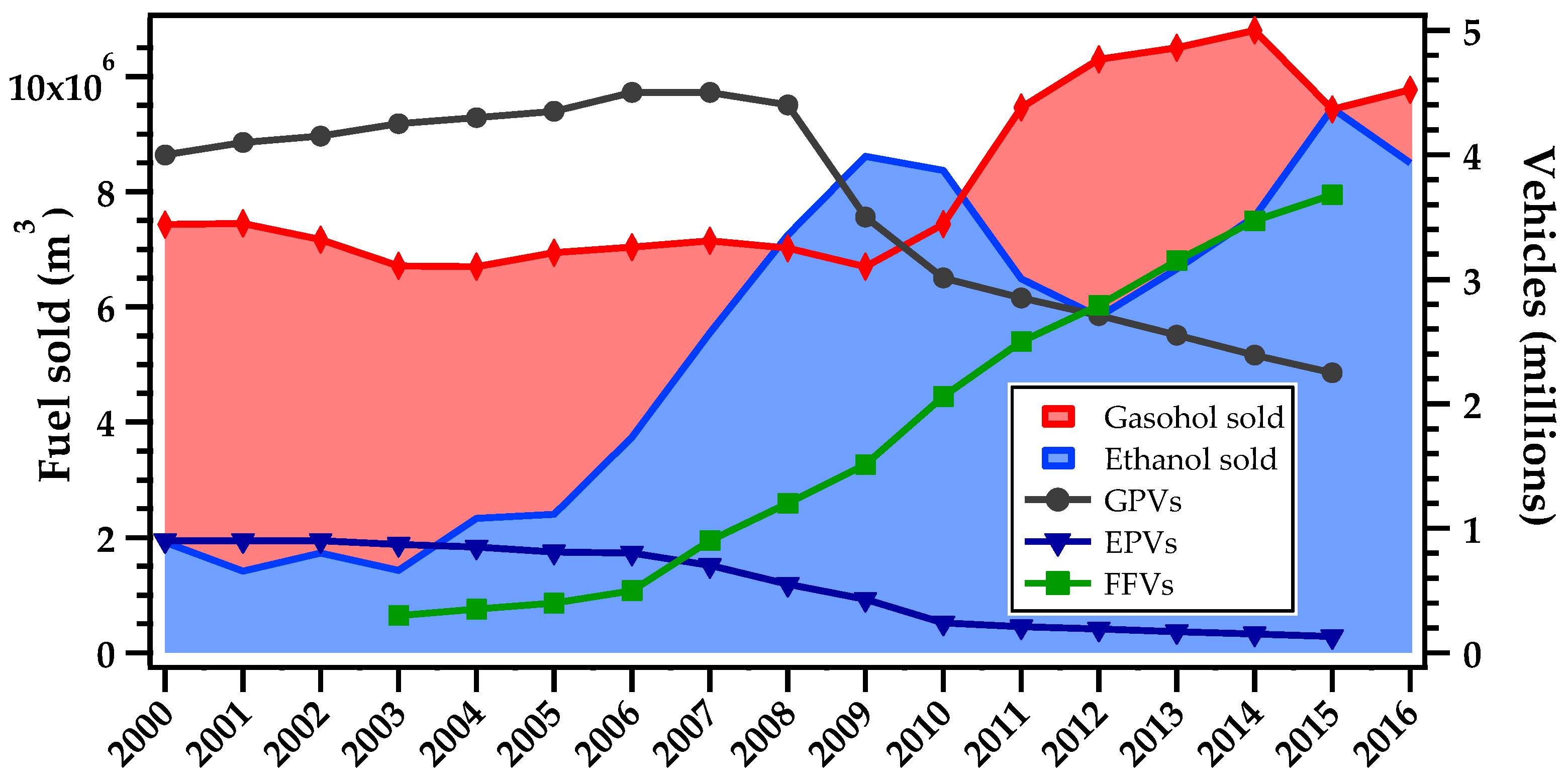
Figure 2.
Seasonal variations in formaldehyde and acetaldehyde concentrations at the Pinheiros air quality monitoring station [24] between 2012 and 2016. The black line represents a formaldehyde/acetaldehyde (F/A) ratio of 1.0, and the green triangles represent the observed F/A ratios.
Figure 2.
Seasonal variations in formaldehyde and acetaldehyde concentrations at the Pinheiros air quality monitoring station [24] between 2012 and 2016. The black line represents a formaldehyde/acetaldehyde (F/A) ratio of 1.0, and the green triangles represent the observed F/A ratios.

Figure 3.
Annual trends in formaldehyde and acetaldehyde concentrations in the Metropolitan Area of São Paulo between 2012 and 2016. The dashed lines indicate the linear fit, and the bars indicate the bars indicate the standard deviation. Source: Pinheiros air quality monitoring station [24].
Figure 3.
Annual trends in formaldehyde and acetaldehyde concentrations in the Metropolitan Area of São Paulo between 2012 and 2016. The dashed lines indicate the linear fit, and the bars indicate the bars indicate the standard deviation. Source: Pinheiros air quality monitoring station [24].

Figure 4.
Formaldehyde and acetaldehyde summer/winter (Su/Win), autumn/winter (Aut/Win), and spring/winter (Spr/Win) ratios in Metropolitan Area of São Paulo. The dashed black line corresponds to a 1:1 ratio between seasons.
Figure 4.
Formaldehyde and acetaldehyde summer/winter (Su/Win), autumn/winter (Aut/Win), and spring/winter (Spr/Win) ratios in Metropolitan Area of São Paulo. The dashed black line corresponds to a 1:1 ratio between seasons.
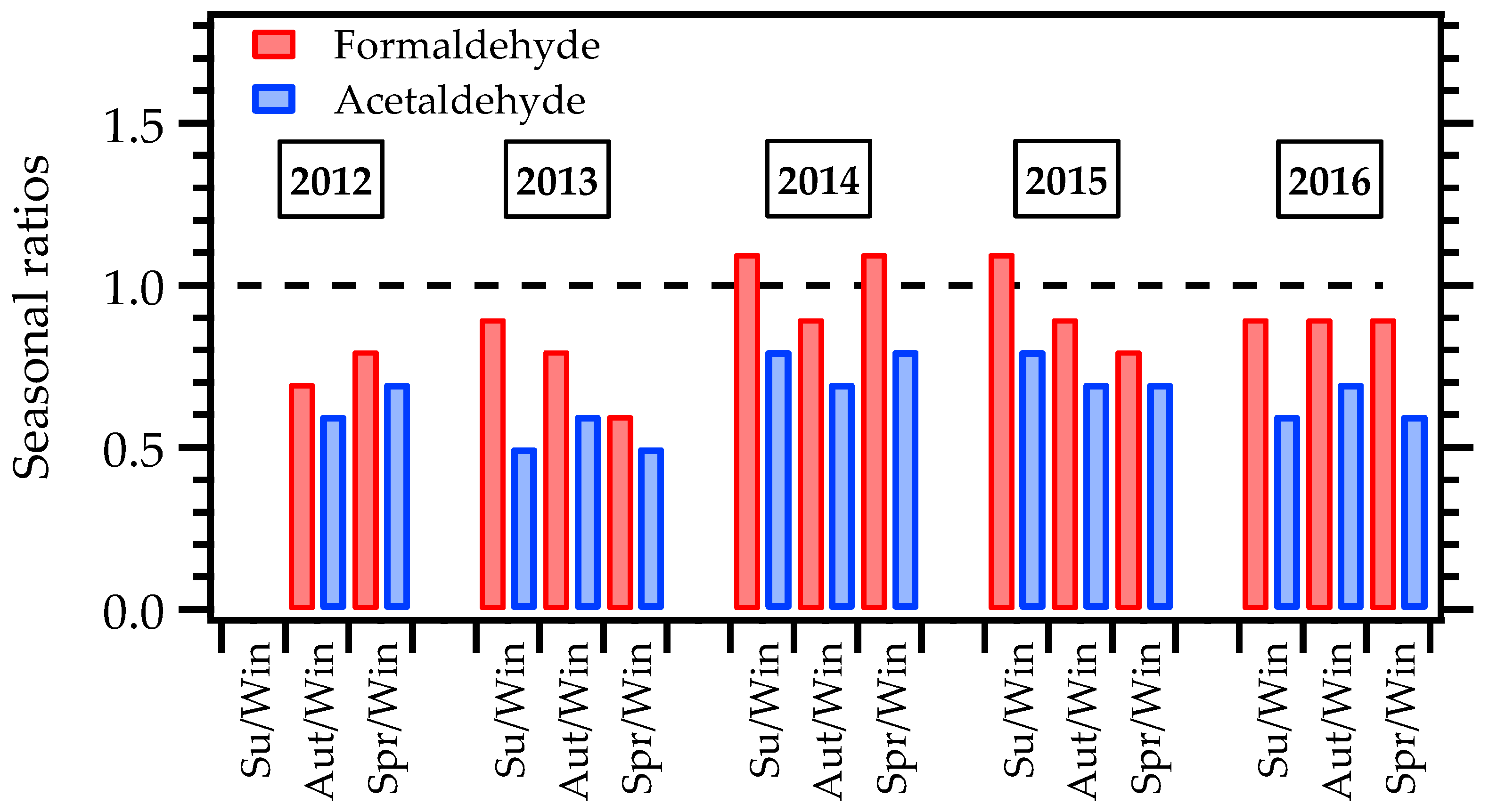
Figure 5.
Seasonal variations in precipitation, temperature, and incoming solar radiation in the Metropolitan Area of São Paulo, between 2012 and 2016 [41].
Figure 5.
Seasonal variations in precipitation, temperature, and incoming solar radiation in the Metropolitan Area of São Paulo, between 2012 and 2016 [41].
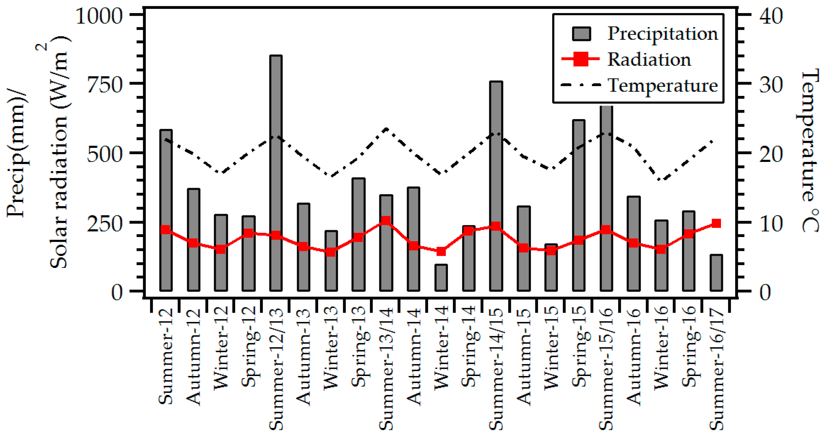
Figure 6.
Box-whisker plots showing the hourly concentrations of NO (a); NO2 (b); ozone O3 (c); and CO (d) at the Pinheiros air quality monitoring station, color-coded by season [24]. The rectangles represent the 25th and 75th percentile values, the lines and squares within the rectangles represent the medians and arithmetic means, respectively. The whiskers indicate the 10th and 90th percentiles.

Figure 7.
Mean propy-equiv (a) and ozone formation potential (OFP) (b) values for concentrations of formaldehyde and acetaldehyde in the Metropolitan Area of São Paulo between 2012 and 2016.
Figure 7.
Mean propy-equiv (a) and ozone formation potential (OFP) (b) values for concentrations of formaldehyde and acetaldehyde in the Metropolitan Area of São Paulo between 2012 and 2016.


Table 1.
Methods and analyzers employed for the measurement of pollutants at the São Paulo State Environmental Protection Agency Pinheiros air quality monitoring station, together with the precision and limit of detection for each method.
Table 1.
Methods and analyzers employed for the measurement of pollutants at the São Paulo State Environmental Protection Agency Pinheiros air quality monitoring station, together with the precision and limit of detection for each method.
| Variable | Formaldehyde and Acetaldehyde | NOx (NO and NO2) | CO | Ozone |
|---|---|---|---|---|
| Method | DNPH method + HPLC technique | Chemiluminescence | Nondispersive infrared photometry | Ultraviolet photometry |
| Analyzer | Shimadzu LC-10A | Thermo-electron (42i) | Thermo-electron (48i) | Thermo-electron (49i) |
| Precision | <1.5% | ±0.4 ppbv | ±0.1 ppmv | ±1 ppbv |
| Detection Limit | 0.01 ppbv | 0.50 ppbv | 0.04 ppmv | 0.50 ppbv |
Table 2.
Mean formaldehyde and acetaldehyde concentrations (ppbv), together with F/A ratios, in the Metropolitan Area of São Paulo (MASP) between 2012 and 2016.
Table 2.
Mean formaldehyde and acetaldehyde concentrations (ppbv), together with F/A ratios, in the Metropolitan Area of São Paulo (MASP) between 2012 and 2016.
| Variable | 2012 | 2013 | 2014 | 2015 | 2016 |
|---|---|---|---|---|---|
| Mean ± SD | Mean ± SD | Mean ± SD | Mean ± SD | Mean ± SD | |
| (Min–Max) | (Min–Max) | (Min–Max) | (Min–Max) | (Min–Max) | |
| Formaldehyde | 4.3 ± 1.2 | 3.9 ± 1.1 | 3.4 ± 1.2 | 3.7 ± 1.4 | 3.7 ± 1.3 |
| (1.7–7.7) | (2.1–6.4) | (1.2–6.2) | (1.3–6.9) | (1.4–6.5) | |
| Acetaldehyde | 3.7 ± 1.5 | 3.5 ± 1.7 | 3.1 ± 1.5 | 2.9 ± 1.5 | 2.8 ± 1.5 |
| (1.4–8.9) | (1.3–8.3) | (0.9–9.1) | (0.6–7.7) | (0.9–7.1) | |
| F/A ratio | 1.2 | 1.1 | 1.1 | 1.3 | 1.3 |
| N of samples | 48 | 35 | 49 | 57 | 57 |
Source: Pinheiros air quality monitoring station [24].
Table 3.
Seasonal comparison of formaldehyde and acetaldehyde mean concentrations (in ppbv), together with the ratios between the seasons, in the Metropolitan Area of São Paulo and in other regions worldwide.
Table 3.
Seasonal comparison of formaldehyde and acetaldehyde mean concentrations (in ppbv), together with the ratios between the seasons, in the Metropolitan Area of São Paulo and in other regions worldwide.
| Pollutant | Summer | Autumn | Winter | Spring | Su/Win | Aut/Win | Spr/Win | Reference |
|---|---|---|---|---|---|---|---|---|
| Locale | ||||||||
| Formaldehyde | ||||||||
| MASP | 4.3 ± 1.4 | 3.5 ± 1.0 | 4.3 ± 1.4 | 3.5 ± 1.2 | 1.0 | 0.8 | 0.8 | This work |
| Londrina, Brazil | 4.11 ± 0.97 | n.a. | 5.07 ± 2.09 | n.a. | 0.8 | n.a. | n.a. | Pinto and Solci. [29] |
| Nanning, China * | 8.7 | 4.1 | 2.5 | 6.4 | 3.5 | 1.7 | 2.6 | Guo et al. [30] |
| Hong Kong (Roadside) * | 5.5 ± 2.2 | 5.9 ± 1.2 | 4.6 ± 1.1 | 4.7 ± 1.0 | 1.2 | 1.3 | 1.0 | |
| Hong Kong (Urban) * | 8.7 ± 2.1 | 3.2 ± 0.8 | 2.9 ± 1.3 | 3.2 ± 1.0 | 3.0 | 1.1 | 1.1 | Cheng et al. [31] |
| Hong Kong (Background) * | 2.1 ± 2.0 | 2.1 ± 0.7 | 1.9 ± 0.5 | 1.6 ± 0.6 | 1.1 | 1.1 | 0.8 | |
| Guangzhou, China * | 11.0 | 3.8 | 4.5 | 4.7 | 2.4 | 0.9 | 1.0 | Lü et al. [32] |
| Guangzhou, China * | 8.9 | n.a. | 3.2 | 5.8 | 2.8 | n.a. | 1.8 | Lü et al. [32] |
| Orléans, France | 3.08 ± 2.21 | 2.28 ± 0.82 | 1.46 ± 0.4 | 2.16 ± 0.59 | 2.1 | 1.6 | 1.5 | Jiang et al. [33] |
| Acetaldehyde | ||||||||
| MASP | 2.8 ± 1.0 | 2.8 ± 1.1 | 4.3 ± 1.8 | 2.8 ± 1.3 | 0.7 | 0.7 | 0.7 | This work |
| Londrina, Brazil | 3.02 ± 1.10 | n.a. | 5.72 ± 2.66 | n.a. | 0.5 | n.a. | n.a. | Pinto and Solci [29] |
| Nanning, China * | 10.4 | 4.6 | 4.7 | 14.9 | 2.3 | 1.0 | 3.3 | Guo et al. [30] |
| Hong Kong (Roadside) * | 1.3 ± 0.8 | 1.6 ± 0.4 | 1.6 ± 0.4 | 1.3 ± 0.4 | 0.8 | 1.3 | 0.8 | |
| Hong Kong (Urban) * | 0.8 ± 0.3 | 1.0 ± 0.3 | 1.1 ± 0.5 | 1.0 ± 0.5 | 0.7 | 0.9 | 0.9 | Cheng et al. [31] |
| Hong Kong (Background) * | 0.5 ± 0.6 | 0.7 ± 0.2 | 0.8 ± 0.2 | 0.5 ± 0.3 | 0.6 | 0.9 | 0.6 | |
| Guangzhou, China * | 5.8 | 3.9 | 3.1 | 1.9 | 1.8 | 1.2 | 0.6 | Lü et al. [32] |
| Guangzhou, China * | 9.5 | n.a. | 2.1 | 3.4 | 4.6 | n.a. | 1.6 | Lü et al. [32] |
| Orléans, France | 1.0 ± 0.5 | 0.7 ± 0.3 | 0.7 ± 0.2 | 1.0 ± 0.3 | 1.6 | 1.0 | 1.5 | Jiang et al. [33] |
* Mean values, expressed as µg/m3 in the literature, were converted to ppbv using 20 °C and 1.0 atm. MASP, Metropolitan Area of São Paulo, n.a.: not available.
Table 4.
Pearson’s correlation coefficients between aldehydes and other pollutants in summer and winter in the Metropolitan Area of São Paulo (2012–2016).
Table 4.
Pearson’s correlation coefficients between aldehydes and other pollutants in summer and winter in the Metropolitan Area of São Paulo (2012–2016).
| Summer | Formaldehyde | Acetaldehyde | NO | NO2 | NOx | CO | Ozone |
| Formaldehyde | 1.00 | 0.92 | 0.38 | 0.49 | 0.43 | 0.42 | 0.65 |
| Acetaldehyde | 1.00 | 0.55 | 0.64 | 0.60 | 0.61 | 0.57 | |
| NO | 1.00 | 0.79 | 0.96 | 0.45 | 0.11 | ||
| NO2 | 1.00 | 0.91 | 0.80 | 0.03 | |||
| NOx | 1.00 | 0.76 | 0.12 | ||||
| CO | 1.00 | 0.26 | |||||
| Ozone | 1.00 | ||||||
| Winter | Formaldehyde | Acetaldehyde | NO | NO2 | NOx | CO | Ozone |
| Formaldehyde | 1.00 | 0.90 | 0.59 | 0.74 | 0.63 | 0.70 | 0.46 |
| Acetaldehyde | 1.00 | 0.79 | 0.79 | 0.82 | 0.85 | 0.33 | |
| NO | 1.00 | 0.61 | 0.99 | 0.90 | 0.12 | ||
| NO2 | 1.00 | 0.67 | 0.71 | 0.39 | |||
| NOx | 1.00 | 0.84 | 0.15 | ||||
| CO | 1.00 | 0.22 | |||||
| Ozone | 1.00 |
© 2017 by the authors. Licensee MDPI, Basel, Switzerland. This article is an open access article distributed under the terms and conditions of the Creative Commons Attribution (CC BY) license (http://creativecommons.org/licenses/by/4.0/).
Share and Cite
MDPI and ACS Style
Nogueira, T.; Dominutti, P.A.; Fornaro, A.; Andrade, M.D.F. Seasonal Trends of Formaldehyde and Acetaldehyde in the Megacity of São Paulo. Atmosphere 2017, 8, 144. https://doi.org/10.3390/atmos8080144
AMA Style
Nogueira T, Dominutti PA, Fornaro A, Andrade MDF. Seasonal Trends of Formaldehyde and Acetaldehyde in the Megacity of São Paulo. Atmosphere. 2017; 8(8):144. https://doi.org/10.3390/atmos8080144
Chicago/Turabian StyleNogueira, Thiago, Pamela A. Dominutti, Adalgiza Fornaro, and Maria De Fatima Andrade. 2017. "Seasonal Trends of Formaldehyde and Acetaldehyde in the Megacity of São Paulo" Atmosphere 8, no. 8: 144. https://doi.org/10.3390/atmos8080144
Note that from the first issue of 2016, this journal uses article numbers instead of page numbers. See further details here.