Dynamic Evaluation of Photochemical Grid Model Response to Emission Changes in the South Coast Air Basin in California

Abstract

This paper describes a study to evaluate the capability of a photochemical grid modeling system to predict changes in ozone concentrations in response to emission changes over a period of several years. The development of regulatory emission control plans to meet air quality standards primarily relies on modeled projections of future-year air quality, although a weight of evidence approach (which takes into account a number of factors including modeling results, model evaluation and other pertinent information such as ambient trends) is recommended and is also typically used as part of the attainment demonstration. Thus, it is important to determine if the modeling system used to project future-year quality can correctly simulate ozone responses to the projected emissions reductions. Uncertainties and errors in modeled projections can lead to erroneous estimates of emissions controls required to attain the standards. We use two existing regulatory modeling databases, employed for forecasting future-year air quality in the South Coast Air Basin (SoCAB) of California, for a number of historical years to evaluate the ability of the system to accurately simulate the observed changes in air quality over a multi-year period. The evaluation results with the older (2012) database show that the modeling system consistently under-predicts the reductions in ozone in response to emission reductions over the years. Model response improves with the newer (2016) database with good agreement at some locations, but the system still tends to under-predict ozone responses by as much as a factor of 2 in recent years for the Basin maximum ozone design value. This suggests that future-year estimates of ozone design values may be overly conservative, resulting in emission controls that are technologically challenging or very expensive to implement. The development of better emission inventories and model inputs is recommended to develop a modeling system that more accurately responds to emission changes. Future regulatory planning should include dynamic evaluation in addition to the traditional operational evaluation of the model to provide more confidence to all stakeholders that the resulting policy decisions are necessary to attain the air quality standards and to protect public health.

1. Introduction

Photochemical grid models (PGMs) are commonly used to predict future-year air quality in regulatory planning to develop emission control strategies for attaining ozone and PM_2.5 air quality standards in a future year. In such applications, the model is applied for a current year and a future year and relative changes in modeled values between the current and future year are used to project current-year measured air quality to future-year air quality under different emission scenarios. Modeling studies have shown that this approach of using relative changes between air quality model simulations of a current year and a future year with observed current-year values provides better estimates of future ozone design values than using the absolute values from a future year simulation [1].

Most regulatory applications of PGMs only evaluate model performance in an operational sense, i.e., they compare model estimates of ozone concentrations for the base year with measurements. They normally do not include a full dynamic evaluation, i.e., an evaluation of the ability of the modeling system (the model inputs and the model itself) to respond correctly to historical and recent changes in precursor emissions, due to time constraints, or due to difficulties in performing such an evaluation because of complications introduced by uncertainties in emission changes and meteorological variability [2,3]. As noted by Hogrefe et al. [4], an operational model performance evaluation does not necessarily provide information on how well the modeling system will perform in the regulatory setting of determining responses to emission changes. Hogrefe et al. [4] recommend placing more emphasis on diagnostic and retrospective dynamic evaluation approaches than on operational performance alone.

The South Coast Air Basin (SoCAB) of California experiences some of the highest ozone concentrations in the U.S. with many exceedances of the National Ambient Air Quality Standards (NAAQS) for ozone [5]. The high concentrations are a result of large precursor emissions from the greater Los Angeles urban area, trapping of pollutants by the marine inversion and mountains on three sides, and high temperatures and abundant sunlight to promote ozone formation photochemically from precursor emissions [6]. The South Coast Air Quality Management District (SCAQMD) has the responsibility for implementing control measures to bring the region into compliance with the NAAQS. Stringent controls on VOC and NO_x emissions over the last 5 decades have resulted in a dramatic improvement in ozone levels in the SoCAB [7,8]. Although the 2008 NAAQS is still exceeded in the Basin on many summer days, the year-to-year ozone reductions have been significant. However, attainment of the more stringent 2015 NAAQS in the future (beyond 2032) presents yet another challenge [8,9].

As part of its efforts to bring the SoCAB region into compliance, the SCAQMD prepares an Air Quality Management Plan (AQMP) approximately every 4 years. The AQMP relies on photochemical grid modeling to determine the effectiveness of emission control measures. Inaccuracies in predicted model responses to emission controls are likely to lead to controls that are either ineffective (if the model over-estimates the response to emission changes) or too stringent (if the model under-estimates the response). Although an operational model performance evaluation for the base modeling year is conducted as part of the AQMP development, there is no assessment of the responsiveness of the model to emission changes over a long time period (i.e., several years). This paper describes a dynamic evaluation of the AQMP modeling system to determine how well the system responds to emissions changes in the SoCAB over a period of 20 to 25 years. A number of dynamic evaluation studies in other contexts have been conducted and those are discussed briefly in the following section.

Previous Dynamic Evaluation Studies

A recommended model evaluation framework [10] consists of four components:

• Operational evaluation: generate statistics of the deviations between model estimates for a simulation year and corresponding observations, and compare the magnitudes of those deviations to selected criteria
• Diagnostic evaluation: test the ability of the model to simulate each of the interacting processes that govern the system
• Dynamic evaluation: test the model’s ability to predict changes in air quality concentrations in response to changes in either source emissions or meteorological conditions
• Probabilistic evaluation: focus on the modeled distributions of selected variables rather than individual model estimates at specific times and locations

Dynamic evaluation looks at retrospective cases to evaluate whether the model has properly predicted air quality responses to known emission and/or meteorological changes [10]. The change in concentration is evaluated instead of the “base” concentration itself, unlike operational and diagnostic aspects of model evaluation. The ability of the model to reproduce historical pollution trends provides confidence in its use for making future year projections.

The U.S. EPA ozone and PM_2.5 modeling guidance [11,12] also discusses this model evaluation framework. For various reasons, including time and resource constraints, most performance assessments of the modeling that underlies regulatory decision-making focus primarily on the first evaluation component, i.e., the operational evaluation that tests how well the model reproduces concurrent observed air quality concentrations for the base year. However, that testing does not evaluate the model in the way it is used in regulatory planning to predict changes in future air quality based on estimates of changes in future emissions [13].

In addition to resource constraints, challenges to conducting a true dynamic evaluation include the influence of year-to-year meteorological variability on the observed trends [10] and the difficulties in developing modeling emission inventories for historical years [14]. Alternative approaches to a multi-year dynamic evaluation include conducting an assessment of model performance for weekday/weekend concentration differences, where mobile source emissions are known to change significantly [10], or assessing the model’s ability to capture the main time variations [14] within the simulated period (e.g., weekly, day-night and/or seasonal). While those approaches provide useful information, they are less appropriate for evaluating a model’s accuracy for multi-year air pollution control planning.

Recognizing the importance of dynamic evaluation in making projections of future-year ozone, a number of dynamic evaluation studies with the U.S. EPA Community Multiscale Air Quality (CMAQ) modeling system [15] have been conducted over the last decade, particularly in the eastern U.S. Those studies are discussed briefly here.

Gilliland et al. [16] took advantage of the large NO_x emission reductions between 2002 and 2005 associated with the EPA’s NO_x State Implementation Plan (SIP) Call, in addition to a more gradual decreasing trend in mobile on-road emissions during that period, to assess the ability of CMAQ to predict changes in ozone. Large decreases in the measured daily maximum 8-h (MDA8) ozone concentrations were reported between 2002 (pre-NO_x SIP Call period) and 2004 and 2005 (post-NO_x SIP Call period). The observed decreases from 2002 to 2004 in O₃ levels were larger than the decreases between 2002 and 2005, because the summer of 2004 was less conducive to ozone formation than the summers of 2002 and 2005 due to cooler and wetter conditions during 2004 [16]. The similar meteorological conditions between 2002 and 2005 better isolated the influence of emission reductions on O₃ concentrations, because NO_x emissions in 2004 and 2005 were comparable and considerably lower than 2002 emissions. CMAQ (versions 4.5 and 4.6) simulations conducted for the summer periods (June through August) of 2002 and 2005 showed that the model-predicted decrease in MDA8 O₃ was less than the observed decrease using 3 different atmospheric chemistry mechanisms (Carbon Bond 4 (CB4); Carbon Bond 2005 (CB05); Statewide Air Pollution Research Center 1999 (SAPRC-99)), although the CB05 mechanism was incrementally better than the other two mechanisms [16]. The comparisons between 2002 and 2004 also showed under-predictions of the ozone reductions from 2002 to 2004, but a significant part of the ozone decrease was due to the differences in meteorology between the two years and the SAPRC mechanism captured the O₃ differences better than the CB4 mechanism. Gilliland et al. [16] suggest that a number of factors may have contributed to the slower response of the model to emission changes, including errors in the NO_x emission inputs or under-prediction of long-range transport of ozone and its precursors.

Pierce et al. [17] conducted a dynamic evaluation of CMAQ using weekend-weekday (WEWD) differences in ozone precursor emissions and 18 years of modeled and observed ozone concentrations. They found that the modeled response of ozone to WEWD differences in emissions was less than the observed response. They attributed the lower response to uncertainties in mobile source NO_x emissions and boundary conditions, as well as to grid resolution.

Napelenok et al. [2] extended the analysis of Gilliland et al. [16] by conducting a dynamic evaluation of CMAQ v4.7.1-predicted ozone changes due to the NO_x SIP Call in the eastern U.S. between 2002 and 2005, and explicitly accounting for known uncertainties in the NO_x emissions inventories. They considered uncertainty in three NO_x emission sectors: area sources, mobile sources, and point sources. Assuming moderate (50%) uncertainty in area and mobile source NO_x emissions and a small uncertainty (3%) in the utility sector, they found that the model was able to reproduce the observed changes in MDA8 O₃ concentrations at more than two-thirds of the monitoring locations. Assuming larger uncertainties (100%) in area and mobile source NO_x emissions, the observed change in the ozone distribution was captured at more than 90% of the sites. Other sources of uncertainty (boundary conditions, VOC emissions, chemistry) were also found to have an impact on model response.

Similarly, Zhou et al. [18] conducted an evaluation of CMAQ 4.7-predicted ozone changes for the NO_x SIP Call region between 2002 and 2006. As in the previous studies [16,17], it was found that observed downward changes in mean NO_x (−11.6 to −2.5 ppb) and 8-h O₃ (−10.4 to −4.7 ppb) concentrations in metropolitan areas in the NO_x SIP Call region were under-predicted by the CMAQ model by 31% to 64% and 26% to 66%, respectively. Sensitivity studies showed that the under-prediction in O₃ improvements could be alleviated by 5% to 31% by constraining NO_x emissions in each year based on observed NO_x concentrations, while adjusting for temperature biases in the meteorological input [18]. Focusing on uncertainties in the chemical reaction rate constants had a smaller influence on the predicted responses.

All of the foregoing dynamic evaluation studies, based on CMAQ versions 4.x, concluded that the modeling system underestimated the observed ozone reductions after the implementation of the NO_x SIP Call, and that modeled ozone responses could be improved by adjusting ground-level NO_x emission inputs, but, even then, observed ozone reductions were still under-estimated. More recently, Foley et al. [1,19] assessed the impacts of the model updates included in CMAQ v5.01 on the dynamic evaluation of ozone predictions for the 2002–2005 NO_x SIP Call period. While the median bias for high summertime ozone decreased in both years compared to previous simulations with CMAQ v4.x, the observed decrease in ozone from 2002 to 2005 in the eastern US continued to be underestimated by the model [1,19]. Sensitivity studies showed that emission controls led to a decrease in modeled high summertime ozone that was nearly twice as large as the decrease attributable to changes in meteorology alone, indicating that the model response to emission reductions during the NO_x SIP Call period continued to be lower than the observed response, even with the updates to the model [1,19].

The dynamic evaluation studies cited above involved regional-scale modeling with grid resolutions of the order of a few kilometers. CMAQ was also used in a hemispheric simulation [20] with a grid resolution of 108 km to model air quality trends across the Northern Hemisphere over a period of 20 years (1990–2010). The air quality simulations were driven by year-specific meteorological fields simulated by the Weather Research and Forecasting (WRF) model and year-specific global anthropogenic emission inventories obtained from the Emission Database for Global Atmospheric Research (EDGAR) for 1990–2008. For 2009 and 2010, emissions for the U.S., Europe and China for 2009 and 2010 were based on the most recent available projections for those years, while emissions for other areas were kept at 2008 levels. The modeled decrease in the annual maxima of daily maximum 8-h average ozone in the eastern U.S. was about 0.5 ppb/year, while the observed decrease was nearly a factor of two higher at about 0.9 ppb/year [20].

The most recent public release of CMAQ (v5.1) incorporates a large number of scientific updates and extended capabilities over the previous release version of the model (v5.0.2). While dynamic evaluation studies with this updated version of CMAQ are not yet published, Appel et al. [21] conducted sensitivity studies for several hypothetical emission reduction scenarios, and found that CMAQ v5.1 tends to be more responsive to reductions in NO_x emissions in predicting ozone reductions than v5.0.2. Appel et al. [21] suggest that this represents an improvement over previous versions of CMAQ, which underestimated O₃ reductions in response to large, widespread emission reductions, as discussed in the studies cited above.

2. Experiments

The dynamic evaluation conducted in this work focused on the two most recent modeling databases available from the regulatory modeling conducted in preparing AQMPs for the SoCAB. Those include the databases for the final 2012 AQMP [22], and the final 2016 AQMP [23]. The latter database became available in August 2016. The modeling conducted with those two databases and their results are described in detail in the corresponding AQMP documents [22,23] and are summarized briefly in the following section.

2.1. The 2012 AQMP and 2016 AQMP Modeling

The 2012 AQMP used CMAQ v4.7.1 for the photochemical modeling, while the 2016 AQMP used CMAQ v5.0.2. Both AQMPs used the same modeling domain (approximately 600 km by 400 km at 4 km resolution in the horizontal, and 18 layers in the vertical) for the SoCAB based on a Lambert Conformal grid projection. Figure 1 shows the modeling domain, the SoCAB, and ozone monitoring stations in the SoCAB. The boundary conditions for this domain were obtained from an outer 12 km resolution CMAQ domain, while the boundary conditions for the outer domain were obtained from the Model for Ozone and Related chemical Tracers (MOZART) global chemical transport model [24]. In the modeling conducted by SCAQMD for the AQMPs, the initial conditions for the CMAQ simulations were based on default clean homogeneous profiles provided in the CMAQ distribution with a five-day spin-up period to offset the homogeneity in initial values [23].

Some of the important differences between the modeling conducted for the 2012 and 2016 AQMPs are:

• CMAQ model versions: v4.7.1 for the 2012 AQMP, and v5.0.2 for the 2016 AQMP.
• Base year (for meteorology and emissions): 2008 for the 2012 AQMP, and 2012 for the 2016 AQMP.
• Ozone season: June through August for the 2012 AQMP, and May through September for the 2016 AQMP.
• Chemistry mechanisms: SAPRC-99 [25] for the 2012 AQMP, and SAPRC-07 [26,27] for the 2016 AQMP.
• Meteorological model versions: the Weather Research and Forecasting Model (WRF) v3.3 was used in the 2012 AQMP, and WRF v3.6 was used in the 2016 AQMP.
• RRF calculations for 8-h ozone attainment demonstrations: the 2012 AQMP modeling followed the EPA (2007) guidance [11], while the 2016 AQMP modeling followed the EPA (2014) guidance [12]. In the 2012 AQMP, all days that met the selection criteria were included in the analysis, while in the 2016 AQMP, the top ten days were selected. Due to the high frequency of ozone episodes in the Basin, the number of days used for the attainment calculations in the 2012 AQMP was significantly higher than ten. For example, the Crestline site, which often determines the Basin design value, typically experiences 50 or more days that would satisfy the selection criteria [23] and all such days were used in the 8-h ozone attainment demonstrations in the 2012 AQMP. The focus on the top ten days in the 2016 AQMP was expected to produce future-year design values that are more responsive to emission reductions [23].

The SCAQMD conducted operational model performance evaluations as part of the development of the final 2012 AQMP and the final 2016 AQMP, and the detailed results of the evaluations can be found in the respective AQMP documents [22,23]. In the 2012 AQMP model performance evaluation, the performance in Zone 4, which includes the Eastern San Gabriel, Riverside and San Bernardino Valleys and represents the Basin maximum ozone concentrations and the primary downwind impact area, showed the best unpaired peak performance with 54 out of 58 days meeting the 20 percent criteria for peak prediction accuracy [22]. Model performance at the Crestline monitor indicated a slight bias towards under-prediction but several peak days were well characterized. Similarly, in the 2016 AQMP model performance evaluation, model estimates of ozone concentrations in the “UrbanReceptor” region, which represents the Basin maximum ozone concentrations and the primary downwind impact zone, were found to agree reasonably well with measured values [23], with a small bias towards under-prediction. While the overall operational evaluation showed reasonable model performance, the ability of the modeling system to accurately predict responses to changes in emissions was not tested.

The ozone attainment demonstration in the 2012 AQMP showed that the projected 2023 baseline design value of 108 ppb would exceed the 1997 federal standard of 80 ppb by 35 percent, and additional reductions in NO_x and VOC emissions, about 64% and 3%, respectively, would be required from the 2023 baseline emissions [22]. In the 2016 AQMP analysis, the 2023 and 2031 baseline scenarios did not lead to attainment of the 1997 and 2008 federal 8-h average scenarios, respectively. The modeling showed that additional NO_x emission reductions of 45% and 60% beyond the 2023 and 2031 baseline values, respectively, would be necessary to meet the standards [23].

2.2. Dynamic Evaluation Approach

As discussed in Section 1, ozone predictions from both versions of CMAQ have been found to be less responsive to NO_x reductions in the eastern U.S., possibly due to uncertainties in a number of variables, such as NO_x emissions, boundary conditions, or model formulation. The objective of this study was to determine whether the two AQMP CMAQ modeling databases could reproduce the ozone reductions in the SoCAB in response to emission reductions over a period of several years. The AQMP modeling databases were provided by the SCAQMD, the regulatory agency responsible for developing the AQMP. Because SCAQMD had already conducted an operational model performance evaluation as part of the AQMP development, we did not conduct a separate operational evaluation of model performance in our study.

The dynamic evaluation conducted in this study compares the changes in modeled ozone design values over a period of several years at monitors in the SoCAB with changes in reported design values based on measurements. The approach to calculate design values in historical years for the evaluation follows the general approach to calculate future-year ozone design values in regulatory modeling and in the 2012 and 2016 AQMPs. That approach is based on guidelines established by the U.S. EPA [11,12] and codified in EPA’s Modeled Attainment Test Software (MATS) tool [28].

In a traditional regulatory application, the base-year measured concentrations at each monitoring site are the anchor point for future-year projected concentrations [11]. The baseline design values are projected into the future using Relative Response Factors (RRFs), i.e., the ratio of the modeled future to current (baseline) predictions at monitors. The future-year predictions are based on projections of future-year emissions. However, the base-year meteorology and boundary conditions are used even for the future year, because it is difficult to predict those variables for a future year. Future-year ozone design values are then estimated at existing monitoring sites by multiplying the RRFs for maximum concentrations in a 3 × 3 matrix of grid cells around each monitor by the observation-based, monitor-specific, base-year design values. Because measurements are not available to evaluate the calculated future-year design values, the approach relies on the implicit assumption that the modeling system correctly calculates the response to changes between the base-year and future-year emissions.

The dynamic evaluation described here followed a similar approach to calculate historical-year and recent future-year (i.e., with available measurements) ozone design values using the 2012 AQMP and 2016 AQMP base years as anchor points. CMAQ simulations were conducted for the historical and recent years (1990, 2000, 2005, 2014 for the 2012 AQMP and 1995, 2000, 2005, 2008 and 2015 for the 2016 AQMP) and the changes between the base year and historical/recent year ozone concentrations at the SoCAB monitors were used to project base-year design values to the corresponding forecast -year design values using the MATS tool. Note that, due to time and resource constraints, the base-year meteorology and boundary conditions were used for all simulations. Thus, the only differences among the various CMAQ simulations were in the emissions specific to each year modeled. To determine the effects of those limitations in our dynamic evaluation approach, we conducted sensitivity studies with alternative meteorological fields and boundary conditions and the results from these studies are also described in this paper.

Two alternative definitions of ozone design values were used in the dynamic evaluation. The first definition is based on the 3-year average of the fourth-highest daily maximum 8-h average ozone (MDA8) concentrations measured at a given monitoring station for the most recent three years. For example, the design value for 2008 is the average of the fourth-highest MDA8 ozone for 2006, 2007, and 2008. This statistic is used to designate areas that are in attainment or non-attainment with the NAAQS for 8-h average ozone. Thus, it is also referred to as the “designation” design value by EPA [11]. Reported design values for the SoCAB are based on that statistic and can be found in the Air Quality Trend Summaries page on the California Air Resources Board website [29].

The second design value definition follows the EPA [11,12] recommendation for modeled attainment tests for future-year projections. The baseline design values under this definition are the simple average of the designation design values for three years, including the baseline inventory year and the two subsequent years. This effectively yields a weighted average of the 4th highest MDA8 ozone concentrations over a five-year period straddling the baseline year. This definition moderates the effects of year-to-year variability in meteorology and emissions. For example, the 5-year ozone design value at a monitoring location for 2008 is a weighted average of the 4th highest MDA8 ozone concentration from 2006 to 2010, with a weighting of 1 for the extreme years (2006 and 2010), a weighting of 2 for the immediately surrounding years (2007 and 2009) and a weighting of 3 for the baseline year (2008).

The following section provides a brief description of the approach used to develop emission files for the specific years modeled for the dynamic evaluation.

2.3. Historical-Year Emissions

Because of the large number of historical years simulated for the dynamic evaluation of the modeling system, we used a relatively simple approach to develop historical-year emissions. In a typical modeling exercise, emission inputs are developed using a detailed source-level emission inventory, spatial surrogates based on geographical data that are representative of the modeling year, and speciation and temporal profiles based on information representative of the modeling year. Such data were not available for this study and developing that information would require significant resources that were beyond the scope of our study. Thus, we developed historical-year emissions by applying scaling factors to adjust model-ready base-year emissions. The ratios of basin-wide criteria pollutant emission totals for each historical year to base-year emission totals were used to determine the scaling factors.

The basin-wide emissions of criteria pollutants for each historical year were obtained from the 2009 and 2013 Almanac inventories, available from the California Air Resources Board (CARB). The 2009 Almanac inventory [30] goes back to 1975 and the 2013 Almanac inventory [31] goes back to 2000. Summer season emissions for the South Coast Air Basin for 2000, 2005, 2008, 2010, 2012 and 2015 were obtained from the 2013 Almanac inventory [31], while 1990 and 1995 emissions were obtained from the 2009 Almanac inventory [30]. The Almanac inventories include both anthropogenic and biogenic emissions and the total emissions were used for scaling. Source-sector specific emissions were not available in the provided AQMP modeling inputs, so the emissions could not be adjusted individually for each sector. The temporal and spatial distributions of emissions were assumed to be unchanged from the base year.

Additionally, we took changes in the composition of volatile organic gas (VOC) emissions over the years into account in developing the historical-year emissions. The composition (and thus, the reactivity) of VOC emissions in the SoCAB has changed over the years. Examples are changes in the VOC composition of motor vehicle exhaust over time due to emissions control devices such as catalytic converters and the changes due to reformulated gasoline. To account for those changes, speciation profiles were applied to each Source Category Code (SCC) or Emission Inventory Code (EIC) in the inventory to calculate the total basin-wide speciated emissions for each VOC species in the model chemical mechanisms (SAPRC-99 for the 2012 AQMP and SAPRC-07 for the 2016 AQMP) summed over all source categories for the base year and each historical year. Scaling factors were then developed for each model mechanism VOC species by calculating the ratio of the total basin-wide speciated base-year and historical-year emissions and applying these scaling factors to the gridded emission inputs. Speciation data used by CARB in its various emissions modeling programs were obtained from the CARB speciation profiles website [32]. A cross-reference file that indicates which Organic Gas profile is assigned to each source category in the inventory for different time periods was also obtained from the same website, and the appropriate cross-reference information was used for each historical year of interest for this study.

For the dynamic evaluation with the 2012 AQMP modeling database, we developed model-ready emissions for 1990, 2000, and 2005 from 2008 base-year emissions using this approach. Note that model-ready emissions for 2014 were already available in the 2012 AQMP database as future-year emissions. Thus, the 2014 emissions are not subject to the assumptions and limitations of the simplified scaling approach adopted in this study. With the newer 2016 AQMP modeling database, model-ready emissions for 1995, 2000, 2005, 2008, and 2015 were developed from the 2012 base-year emissions.

Table 1. Domain-wide average emissions (tons per day) from scaling 2008 emissions (2012 AQMP).

Pollutant	1990	2000	2005	2008
NOx	2759	1889	1528	1473
CO	21,192	9388	6500	6560
TOG	8872	11,555	10,390	4552
NH3	360	360	360	360
SO2	355	223	211	160
PM2.5	356	234	228	280
PM10	1209	683	671	987

and

Table 2. Domain-wide average emissions (tons per day) from scaling 2012 emissions (2016 AQMP).

Pollutant	1995	2000	2005	2008	2012	2015
NOx	3086	2472	1999	1614	1158	1022
CO	14,747	8599	5954	5185	4066	3546
TOG	7989	8952	6363	5637	4676	4433
NH3	308	308	308	308	308	308
SO2	240	213	202	127	71	71
PM2.5	350	270	262	239	217	211
PM10	1964	995	987	955	906	937

summarize the average emission rates over the modeling domain in Figure 1 for the different years simulated with the 2012 and 2016 AQMP modeling databases, respectively, using the simplified approach.

3. Results and Discussion

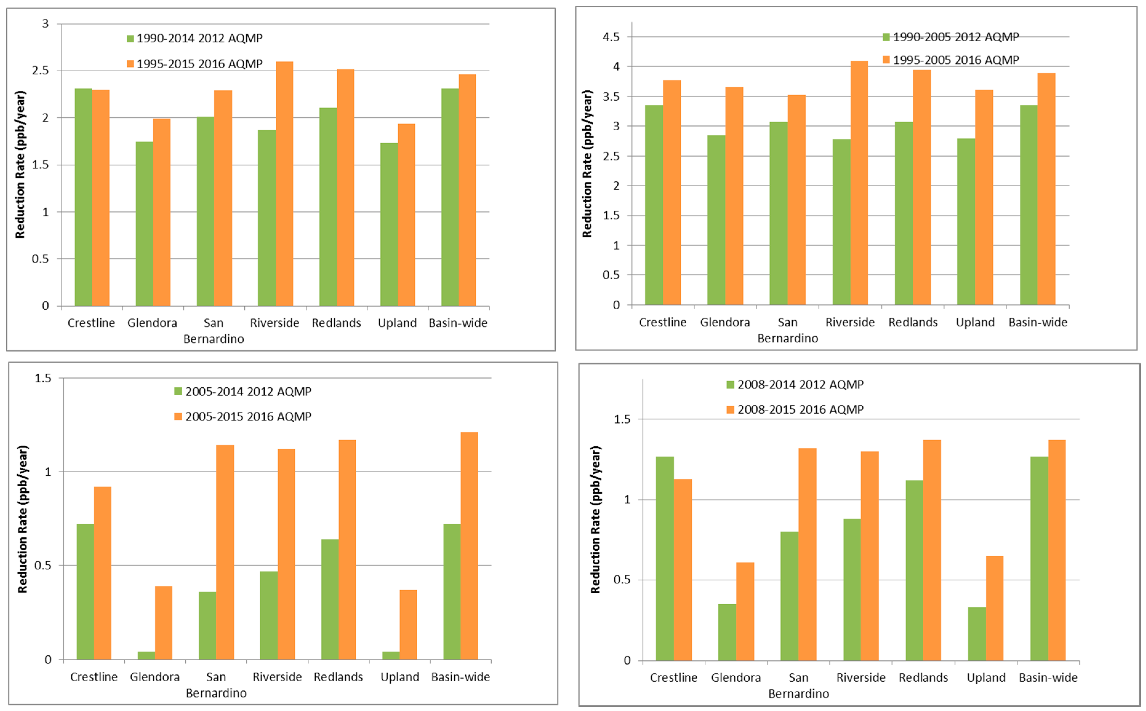
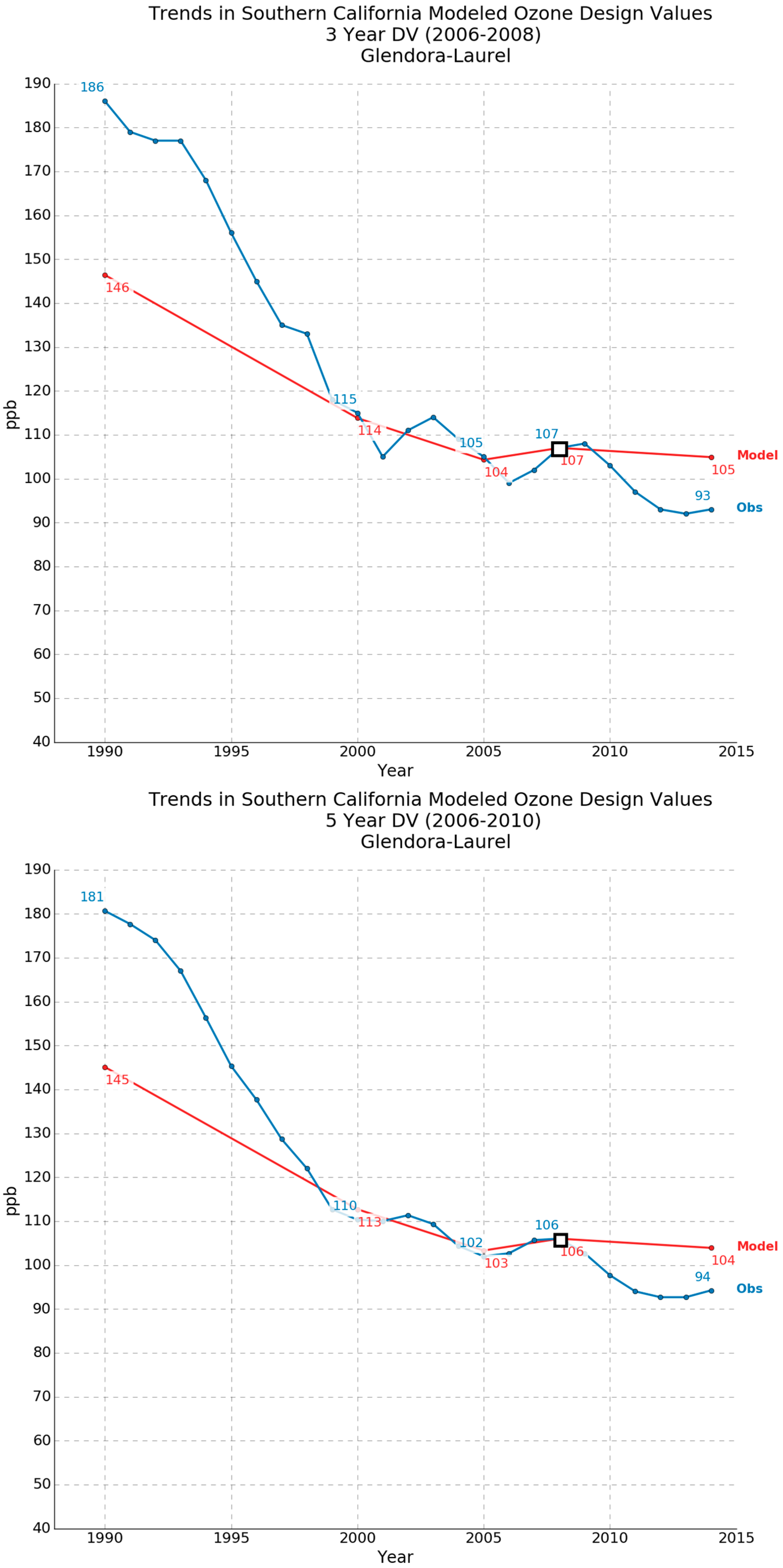
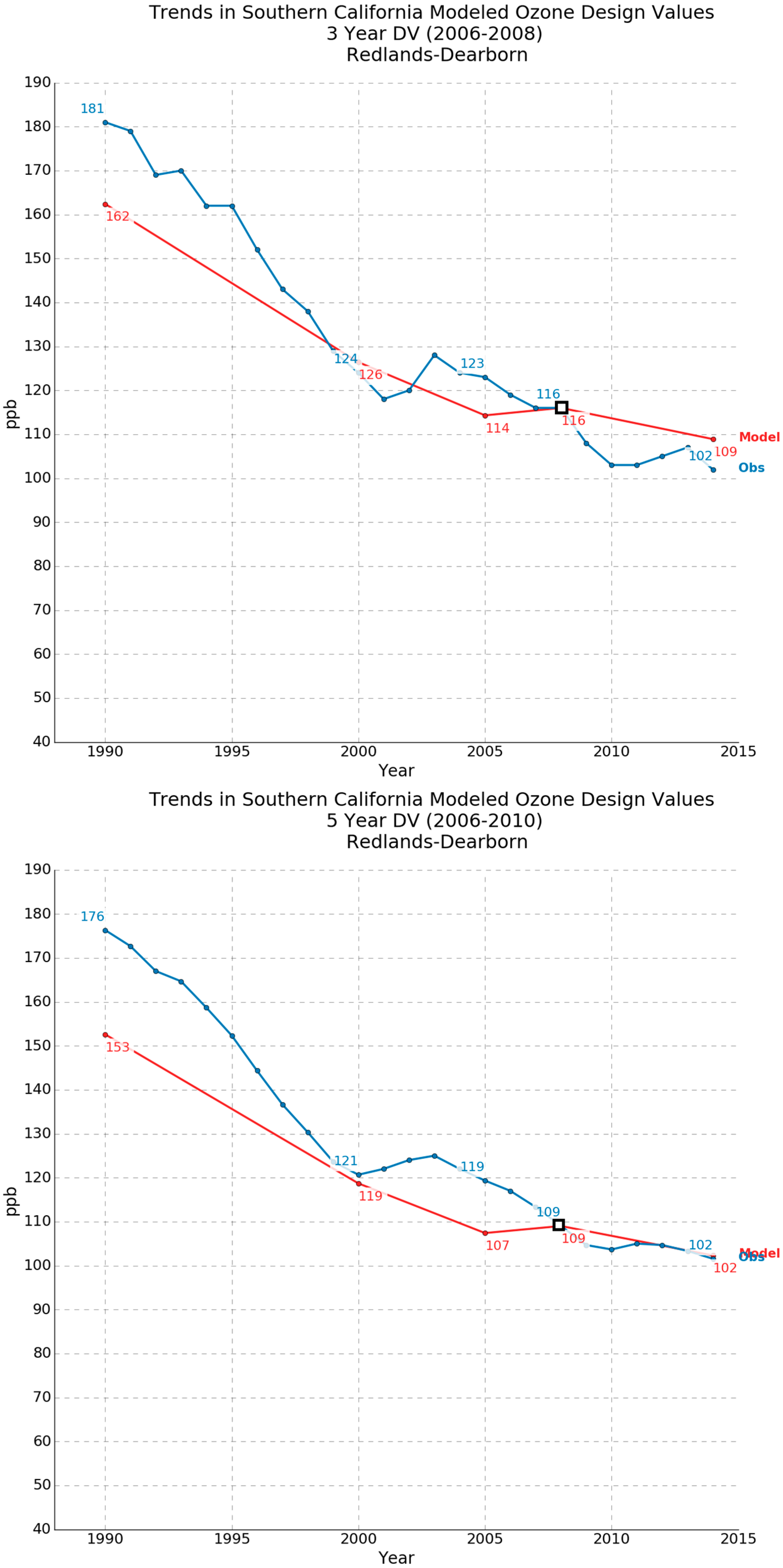
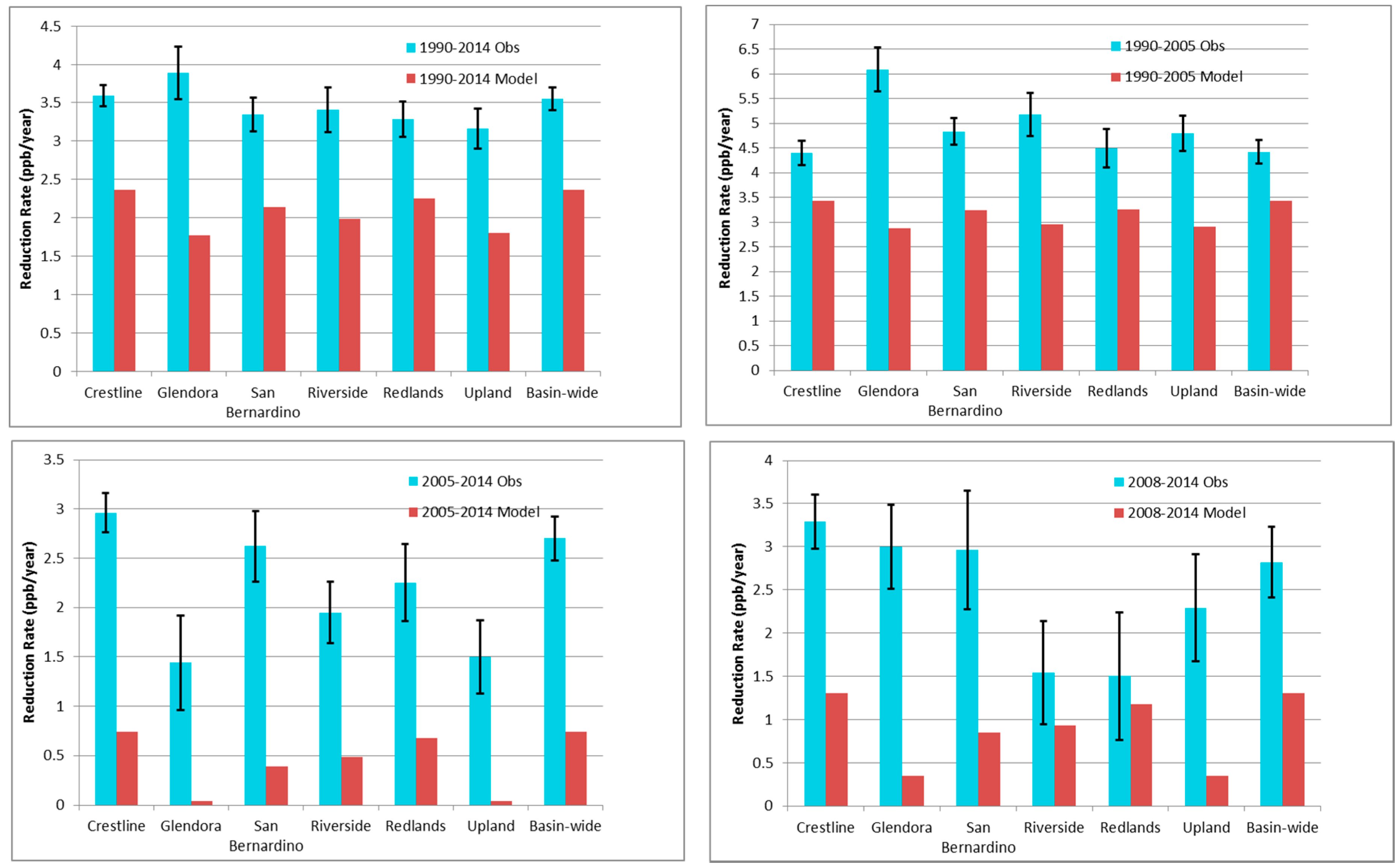
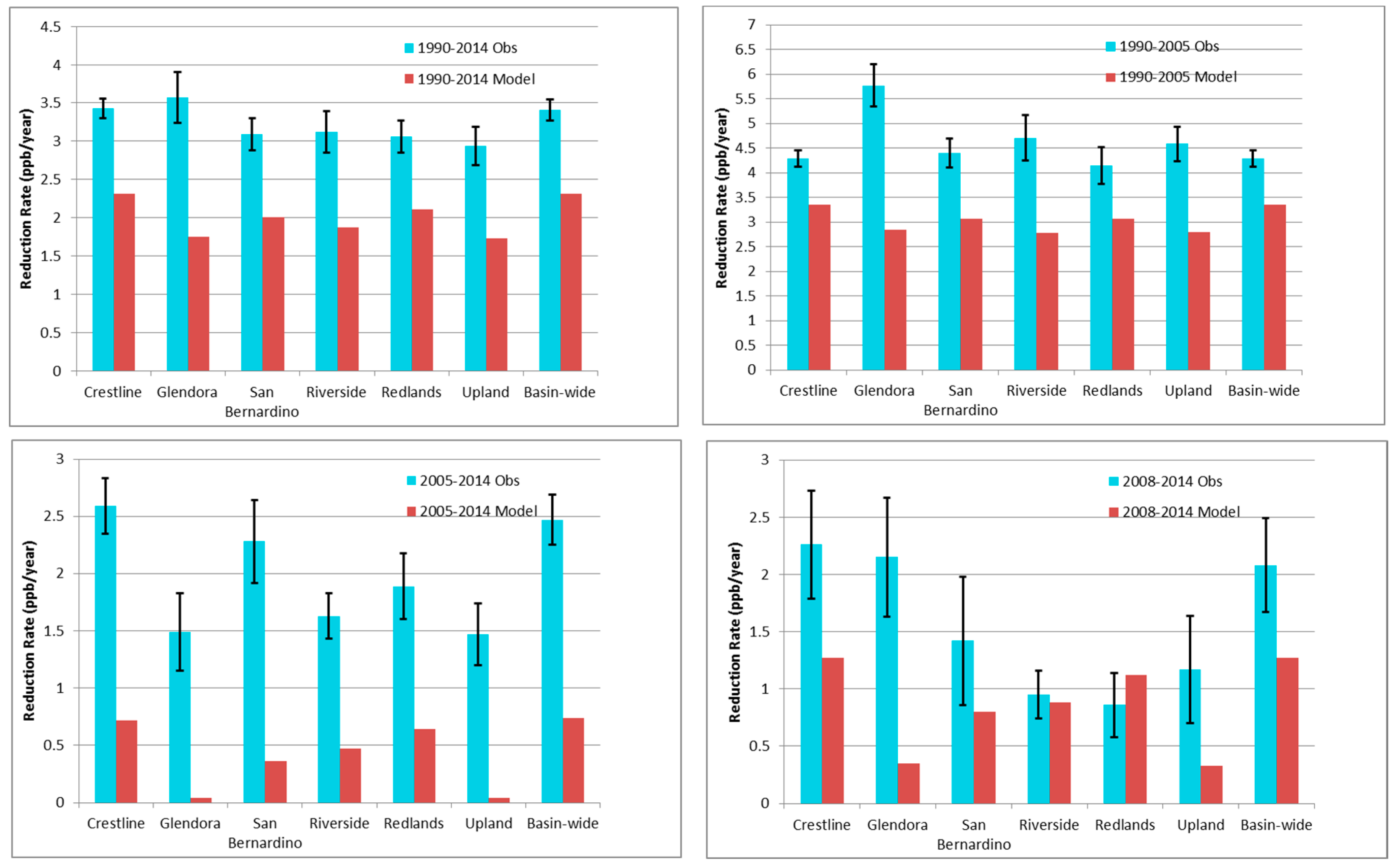
3.1. Dynamic Evaluation Using 2012 AQMP Database

The dynamic evaluation conducted with the 2012 AQMP modeling database compared modeled and measured changes in 3-year and 5-year ozone design values from 1990 to 2014 using CMAQ 4.7.1 simulations for 1990, 2000, 2005, 2008, and 2014. Model-ready emission files for 2008 and 2014 were already available as part of the 2012 AQMP database. Emissions for the other three years were developed from the baseline (2008) emissions using the approach described in the previous section. Note that the 2008 emissions included corrections for the economic recession that began in December 2007 and ended in June 2009 [22].

The dynamic evaluation results are presented for selected monitors in Los Angeles County and the inland valley areas in San Bernardino and Riverside Counties (see Figure 1 for monitor locations), where high ozone concentrations in the SoCAB historically have been measured. In particular, the basin design values (the 3-year designation design values for the SoCAB) over most of the last 20 years have been determined by the Crestline monitor at Lake Gregory in the central San Bernardino Mountains. In recent years, the Redlands monitor in the east San Bernardino Valley also has sometimes determined the basin design values. Other locations that frequently experience high ozone levels in the SoCAB are the Santa Clarita monitor in northern Los Angeles County, the Glendora monitor in the east San Gabriel Valley in Los Angeles County, the Fontana and San Bernardino monitors in the central San Bernardino Valley, the Upland monitor in the northwest San Bernardino Valley, and the Riverside-Rubidoux and Banning Airport monitors in Riverside County. All these monitors are located in suburban and semi-rural areas that frequently experience ozone episodes, and are approximately 50 to 100 km downwind of the high emissions generated in the Los Angeles urban area.

Figure 2, Figure 3 and Figure 4 show the observed and modeled trends in 3-year and 5-year ozone design values at 3 selected monitors from 1990 through 2014. Those three monitors have determined the basin design value during this period. At the Crestline monitor (Figure 2), which has determined the basin design value for all but three years over this period (1990, 2013 and 2014), there is a rapid decline in observed ozone design values from 1990 to 2000 with intermittent increases due to meteorological variability. The effect of the meteorological variability is smoothened out in the 5-year design values, shown in the bottom panel of Figure 2. The model design values also show a steady decline, but the rate of the modeled reduction is lower than the observed reduction rate. The 5-year ozone design value from measurements at the Crestline monitor drops by 48 ppb between 1990 and 2000, while the modeled design value drops by 37 ppb during the same period. Fujita et al. (2013) [5] have noted that the rate of decline slows between 2000 and 2008 as the decline in VOC/NO_x ratios begins to reverse, and this behavior is seen in both the observed and modeled ozone trend lines. Between 2008 and 2014, the observed 3-year design values again fall more rapidly than the modeled values. This disparity between the observed and modeled ozone reduction rates in recent years is also seen in the 5-year design values, but the 5-year observed ozone design value in 2014 shows an uptick, primarily due to higher ozone levels measured in 2014, 2015 and 2016 as a result of abnormally hot stagnant weather and wildfires. For example, the 4th highest MDA8 ozone at Crestline was 100 ppb in 2013 and 103, 108 and 117 in 2014, 2015, and 2016, respectively. Those variations are generally not reproduced in the modeled design values since the model results are based on a single meteorological year (2008).

The results for the other monitoring locations show similar differences between the observed and modeled ozone trends. At the Glendora monitor (Figure 3), which determined the basin design value in 1990, the modeled responses of both 3-year and 5-year ozone design values are significantly lower than the measured responses during the beginning and end of the 24 year period, but similar from 2000 to 2005 and from 2005 to 2008. The results are similar for the Redlands monitor, which determined the basin design values in 2013 and 2014, as shown in Figure 4.

In general, for all the selected monitors, the overall downward trends in ozone design values over long-term periods tend to be underestimated by the model. This is seen in Figure 5 and Figure 6, which summarize the changes in 3-year and 5-year ozone design values, respectively, as a reduction rate (ppb/year) over 3 long-term (~10 years or more) time periods and the most recent time period (2008–2014) for the basin design value as well as at the Crestline, Glendora and Redlands monitors, and at three other downwind monitors that experience high ozone concentrations. The reduction rates are determined by the best fit lines for the observed and modeled trends. The error bars in the observed values provide a measure of the standard error associated with the calculation of the slope of the best fit line for the observations.

For the 25 year period, the observed rates of reduction in the 3-year and 5-year ozone design values at the Crestline monitor are 50% higher than the modeled rates. Similar differences are noted in the basin design values. For the more recent 6 year period from 2008–2014, the observed reduction rates in the 3-year ozone and 5-year design values are 2.5 times and 1.8 times higher than the modeled rates, respectively, at the Crestline monitor. The observed rates of reduction in the 3-year and 5-year ozone Basin maximum design values for the recent 6-year period from 2008 to 2014 are more than a factor of 2 and 1.6 times higher than the modeled rates of reduction, respectively. Note that the errors in the calculated observed ozone reduction rates for the recent 6-year period are generally larger than the errors for the longer term periods. For example, the measured ozone reduction rates at the Riverside and Redlands monitors have errors of 40 to 50%, resulting in a possible range of values from 0.94 to 2.14 ppb/year and from 0.76 to 2.24 ppb/year, respectively. The modeled reduction rates at these two monitors are 0.93 ppb/year and 1.18 ppb/year, respectively, and are within the ranges of the measured rates. However, for the Crestline monitor design value and for the maximum Basin design value, the errors are smaller (10 to 15%) and the modeled values are much smaller than the low end of the observed range of values.

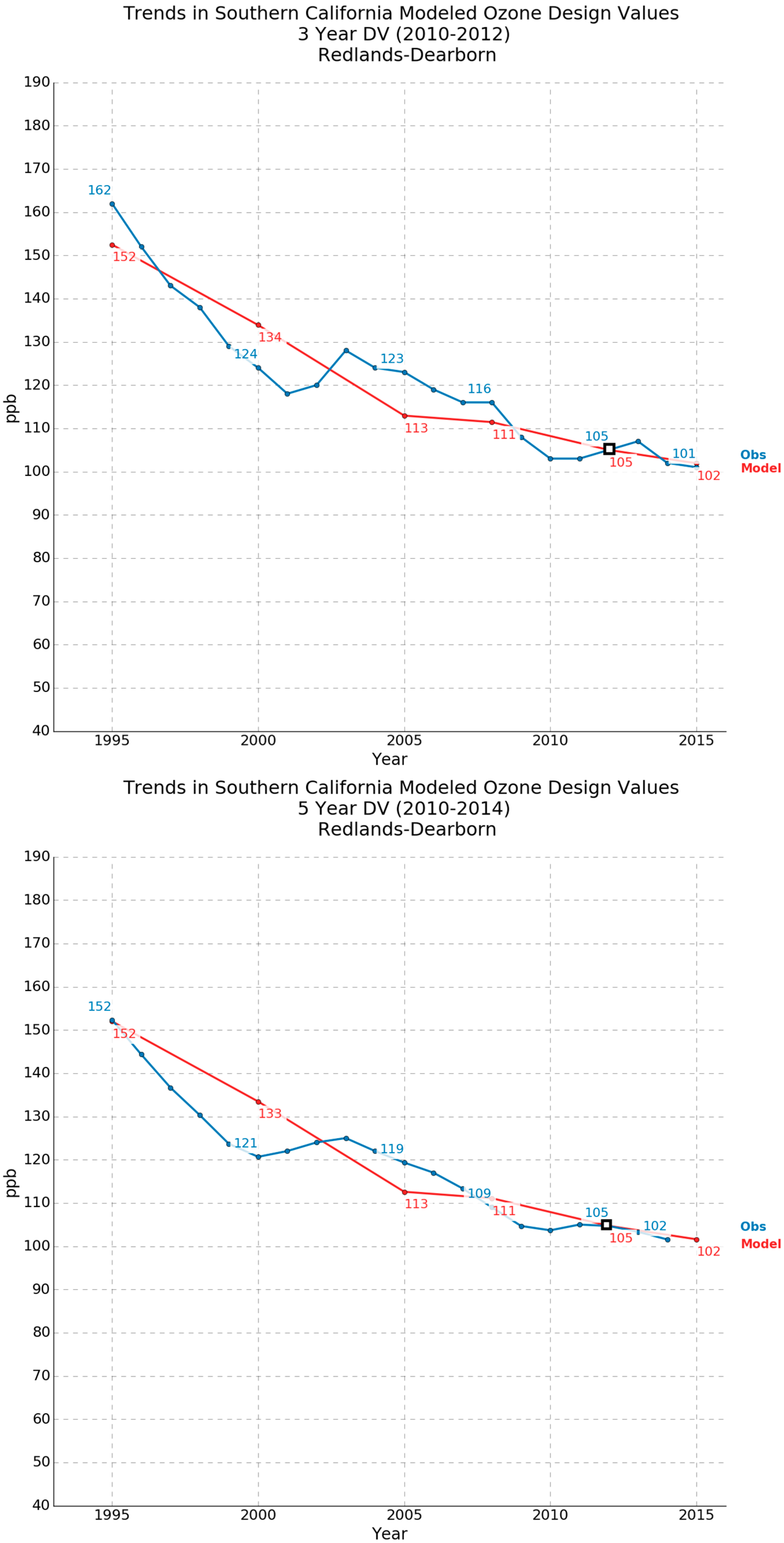
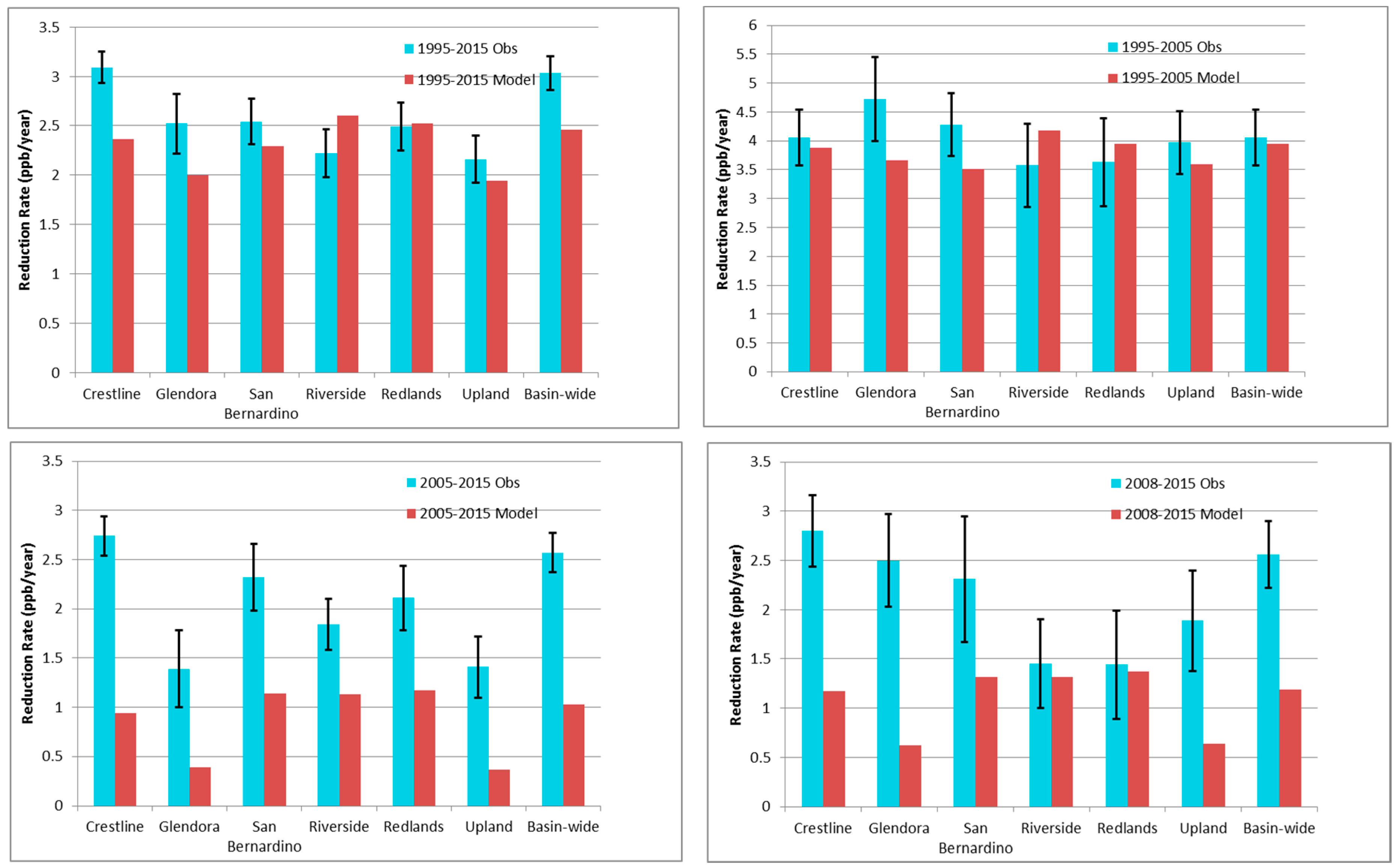
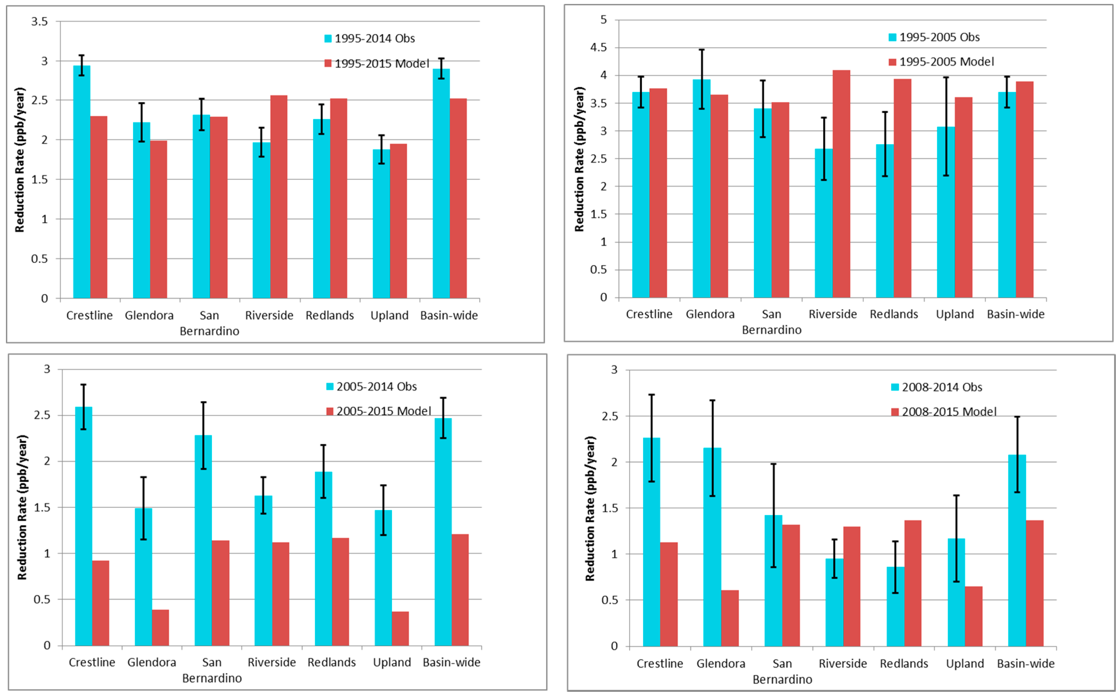
3.2. Dynamic Evaluation Using 2016 AQMP Database

The 2016 AQMP database was used to conduct CMAQ 5.02 simulations for 1995, 2005, 2008, 2012, and 2015, using the 2012 baseline year meteorology. Emissions for the historical years (1995, 2005, 2008) and 2015 were developed as described in Section 2.3. The results are presented for the same set of monitors that were discussed in Section 3.1, since those monitors typically experience the highest ozone levels in the SoCAB.

Figure 7, Figure 8 and Figure 9 compare the observed and 2016 AQMP modeled ozone trends for the 3-year and 5-year ozone design values at Crestline, Glendora, and Redlands, respectively. As mentioned previously, there is an increase in observed 5-year ozone design values at most monitors in 2014 due to increases in measured 4th highest MDA8 ozone levels in 2014, 2015 and 2016. Those increases are not reproduced in the modeled results, which use a single meteorological year for the ozone projections and do not include the wildfire events and other conditions contributing to the measured high ozone levels in these recent years.

The modeled trends for Crestline (Figure 7) using the 2016 AQMP database show that the modeling system is more responsive than the 2012 AQMP system. The increase in responsiveness is also seen for the Glendora (Figure 8) and Redlands (Figure 9) monitors, particularly the Redlands monitor. The modeled and measured reduction rates in 3-year and 5-year ozone design values are compared in Figure 10 and Figure 11, respectively. Those comparisons show that the newer modeling database shows increased responsiveness over the long-term period (1995–2015). At some monitors, such as Redlands and Upland, there is good agreement between the observed and modeled ozone reduction rates over this period, illustrating the improvement in model response with the newer database. However, the modeling system still tends to underestimate the observed ozone multi-year reductions at Crestline and for the Basin maximum design values. For the Basin maximum design value, the difference between long-term observed and modeled reduction rates of about 0.5 ppb/year translates to a difference of about 10 ppb over 20 years.

Some of the improvement in model performance in predicting long-term ozone trends, as compared to the 2012 AQMP database, is likely due to increased model responsiveness and also due to the uptick in the measured ozone design values during 2014 to 2016, as mentioned previously. At some stations, such as Riverside and Redlands, the modeled reduction rates in 3-year and 5-year ozone design values are actually higher than the observed rates during some periods. However, it should be noted that the recent observed ozone trends at Riverside and Redlands generally have a shallower slope than at the other monitoring locations, suggesting that these areas are less NO_x-limited than other remote areas, such as Crestline. The reduction rates in the basin-wide maximum ozone design values, which are predominantly determined by the Crestline monitor, and which determine if the region is in violation of the NAAQS, are still consistently underestimated, although to a lesser extent than with the 2012 AQMP modeling database. For the most recent period (2008 to 2015), the observed reduction rates in both the 3-year and 5-year ozone design values at Crestline are still more than a factor of 2 higher than the modeled rates. For this same period, the observed reduction rates in the 3-year and 5-year basin design values are more than a factor of 2 and 1.4 times higher than the modeled rates, respectively.

Figure 12 and Figure 13 compare the responsiveness of the two AQMP modeling databases for the 3-year and 5-year ozone design values, respectively. Those comparisons confirm that, for the most part, the 2016 AQMP modeling database is more responsive to multiyear emission changes than the 2012 AQMP database. At the Crestline monitor, the two AQMP responses are comparable for a 20 to 25 year period (1990s to 2015) and for the most recent period (2008 to 2015). This is also true of the basin-wide design value, which is often the same as the Crestline design value.

The above results indicate that the 2016 AQMP modeling system appears to be more responsive than the modeling system used in the previous 2012 AQMP. While this is encouraging, the system still under-predicts ozone reduction rates for the basin design values and at the monitor which has predominantly determined the basin design values over the last 25 years. As discussed in Section 2.2 and Section 2.3, there are some limitations in the approach adopted in our study to perform the dynamic evaluation, particularly in the specification of base-year meteorology and boundary conditions for historical years, and in the relatively simplified approach used to develop model-ready emission inputs for the historical years. While those simplifications were adopted due to the limited scope of this study, we conducted some sensitivity studies with the 2016 AQMP modeling system to determine how uncertainties in our modeling approach might impact the dynamic evaluation results, and to determine how the responsiveness of the modeling system would be influenced by these uncertainties. The following sections provide additional details on the sensitivity studies and their results.

3.3. Meteorology and Boundary Condition Sensitivity Studies

For testing the influence of meteorology on the dynamic evaluation results, we used the 2008 meteorology that was available from the 2012 AQMP to conduct base year (2012) and projected year (2008 and 2015) simulations using the 2016 AQMP modeling database. The emission files for the projected years were scaled from the 2012 emissions as described in Section 2.3 and used in the dynamic evaluation described in Section 3.2. For testing the influence of boundary conditions, we reduced ozone boundary conditions by 20% to create a scenario where the influence of emission changes would be larger than in the baseline dynamic evaluation discussed previously.

The results for the 3-year design values at selected monitors and the basin design value are summarized in

Table 3. 2016 AQMP ozone reduction rates (ppb/year) in 3 year ozone design values for the 2008–2015 period for the baseline case and for the meteorology and boundary condition sensitivity studies.

Monitor	Observed	2016 AQMP
		Baseline	2008 Meteorology	O3 BCs Reduced by 20%
Crestline	2.8	1.2	1.0	1.4
Glendora	2.5	0.6	0.3	0.7
Redlands	1.4	1.4	1.3	1.4
Basin-wide	2.6	1.2	1.1	1.4

for the meteorology and boundary conditions sensitivity studies. The results from this meteorology sensitivity study show a small impact on ozone design values in the projected years for all monitoring stations, with the 2008 meteorology resulting in a slightly less responsive system. As expected, reducing the ozone boundary conditions by 20% results in a slightly more responsive system, indicating that uncertainties in boundary conditions can influence future-year model projections to some extent. The Redlands monitor shows the least sensitivity to both changes in meteorology and boundary conditions. As shown in Table 3, the reduction rates of modeled basin 3-year ozone design values are about a factor of 2 lower than the observed reduction rates for the baseline case as well as the two sensitivity studies.

While these sensitivity studies provide useful information on the effects of meteorology and boundary conditions on model response, they do not account for year-to-year changes in these variables that will also have an effect on model response. For example, Porter et al. [33] report that meteorology accounts for 39–92% of year-to-year ozone variability in the western U.S. For the 20 to 25 year periods considered in our analysis, the large reductions in emissions are likely to have played a more dominant role than meteorological or boundary condition variations on the large ozone reductions over this period. Nevertheless, using year-specific meteorology and boundary conditions would provide additional insight into the dynamic performance of the modeling system, but was outside the scope of our current study.

3.4. Emissions Sensitivity Study

To support the development of a scenario for emissions sensitivity modeling, we performed emissions reconciliation analyses that compared molar pollutant ratios (e.g., VOC/NO_x and CO/NO_x) derived from ambient monitoring data, emissions inputs used for the baseline AQMP 2016 photochemical modeling, and CMAQ model outputs. Emissions reconciliation techniques have previously been applied to evaluate emissions inventories in the SoCAB, and have generally indicated that VOC/NO_x ratios derived from ambient measurements are higher than corresponding ratios derived from emissions data or photochemical modeling results [5].

The analysis performed on the 2012 AQMP modeling platform focused on 6 monitoring sites around the SoCAB that measured ozone, VOC, and NO_x concentrations in 2012. Results showed that ambient measurement-derived VOC/NO_x ratios were 1.7 to 3.1 times higher than corresponding ratios derived from gridded emissions data for the area around each monitoring site. VOC/NO_x ratios derived from CMAQ outputs showed closer agreement with ratios derived from ambient measurements; however, discrepancies were still found at some sites. For example, the ambient measurement-derived VOC/NO_x ratio at the Los Angeles North Main site, which has a high density of local emissions dominated by motor vehicles, was 2.4 times higher than the ratio derived from CMAQ outputs. CMAQ also significantly under-predicted VOC concentrations at this site with a normalized mean bias of −75%, while the predicted NO_x was in closer agreement with observations with a normalized mean bias of less than 10%. Based on those results, we conducted a sensitivity dynamic evaluation of the 2016 AQMP modeling database by increasing basin-wide VOC emissions by a factor of 2 for the base year (2012) and two projected years (2008 and 2015). Although the VOC under-prediction in 2012 does not necessarily mean that VOC is under-predicted by the same amount in the two projected years, doubling the VOC emissions for all 3 years preserves the emission scaling ratios between the base year and the projected years.

The results from that analysis are summarized in

Table 4. 2016 AQMP ozone reduction rates (ppb/year) in 3 year ozone design values for the 2008-2015 period for the baseline case and for VOC emissions sensitivity study.

Monitor	Observed	2016 AQMP
		Baseline	Double VOC Emissions
Crestline	2.8	1.2	2.3
Glendora	2.5	0.6	2.2
Redlands	1.4	1.4	2.7
Basin-wide	2.6	1.2	2.5

, which shows that doubling VOC emissions has a dramatic effect on the responsiveness of the 2016 AQMP modeling system for the 2008–2015 period. The predicted ozone reduction rates increase by a factor of 2 or more. The modeled reductions in the basin design value and the design values at the Crestline and Glendora monitors are quite comparable to the observed values. At the Redlands monitor, where the modeled reduction rates were previously comparable to the observed rates for the baseline case, the increase in responsiveness of the modeling system now results in more rapid modeled reductions than the observed reductions. As discussed previously, observed ozone design value reductions at this location during the 2008–2015 period are smaller than at Crestline, which is in a remote NO_x-limited area.

4. Conclusions

The dynamic evaluation results show that recent modeling databases used for regulatory modeling in the South Coast Air Basin generally underestimate the changes in basin ozone design values in response to precursor emission changes. At the Crestline monitor, the predicted rate of ozone reduction in recent years is about a factor of two lower than the measured decline in ozone levels. Since that monitor often determines the basin-wide design value, this suggests that reductions in future-year ozone concentrations for attainment demonstrations in the SoCAB could be underestimated. A modeling system that responds more accurately to emission changes would provide more confidence to all stakeholders that policy decisions resulting from the modeling are necessary to attain the air quality standards and to protect public health.

The 2016 AQMP modeling database appears to be somewhat more responsive to emission changes than the 2012 AQMP database, but is still less responsive when compared to the observed basin design value trends. The improved responsiveness of the 2016 modeling system is likely due to model improvements (CMAQ v5.0.2 in the 2016 AQMP versus CMAQ v4.7.1 in the 2012 AQMP) and more accurate emission inventories. Nevertheless, the dynamic evaluation results with the 2016 AQMP database suggest that additional improvements are necessary to obtain more accurate responses to future emission changes. While the simplified approach to dynamic evaluation in this study introduces some limitations and uncertainties in the results, the sensitivity studies conducted with the 2016 AQMP database to determine the influence of those approximations indicate that the overall modeling system is still “stiff” in responding to emission changes as compared to the observed responses. The sensitivity studies with alternative meteorology and reduced boundary conditions showed an impact of less than 10% on modeled basin design value ozone trends. As noted in the dynamic evaluation studies conducted by Foley et al. [1,19], large emission reductions lead to larger decreases in ozone than variability in meteorology. Similarly, the work of Gilliland et al. [16] showed that modeled ozone decreases due to emission changes between two similar meteorological years were lower than observed ozone decreases. On the other hand, our sensitivity study in which VOC emissions were increased to make modeled VOC/NO_x ratios more consistent with ambient measurements at urban locations resulted in a dramatic improvement in model responsiveness.

The dynamic evaluation study conducted by Napelenok et al. (2011) [2] clearly illustrates that ozone changes predicted by the model in response to emission reductions are sensitive to a large number of variables. The sensitivity studies conducted by Appel et al. [21] suggest that CMAQ v5.1 tends to be more responsive to reductions in NO_x emissions in predicting ozone reductions than CMAQ v5.0.2. The sensitivity studies conducted as part of this study also show that more realistic boundary conditions and more accurate emission inventories are another area of improvement for future regulatory planning. A detailed dynamic evaluation of future regulatory modeling databases also would provide additional confidence to stakeholders regarding the reliability of future-year model predictions. As a result, those types of additional dynamic evaluations are recommended.

References

1. Foley, K.M.; Dolwick, P.; Hogrefe, C.; Simon, H.; Timin, B.; Possiel, N. Dynamic evaluation of CMAQ part II: Evaluation of relative response factor metrics for ozone attainment demonstrations. Atmos. Environ. 2015, 103, 188–195. [Google Scholar] [CrossRef]
2. Napelenok, S.L.; Foley, K.M.; Kang, D.; Mathur, R.; Pierce, T.; Rao, S.T. Dynamic evaluation of regional air quality model’s response to emission reductions in the presence of uncertain emission inventories. Atmos. Environ. 2011, 45, 4091–4098. [Google Scholar] [CrossRef]
3. Cohan, D.S.; Napelenok, S.L. Air quality response modeling for decision support. Atmosphere 2011, 2, 407–425. [Google Scholar] [CrossRef]
4. Hogrefe, C.; Civerolo, K.L.; Winston, H.; Ku, J.-Y.; Zalewsky, E.E.; Sistla, G. Rethinking the assessment of photochemical modeling systems in air quality planning applications. J. Air Waste Manag. Assoc. 2008, 58, 1086–1099. [Google Scholar] [CrossRef] [PubMed]
5. Fujita, E.M.; Campbell, D.E.; Stockwell, W.R.; Lawson, D.R. Past and future ozone trends in California's South Coast Air Basin: Reconciliation of ambient measurements with past and projected emission inventories. J. Air Waste Manag. Assoc. 2013, 63, 54–69. [Google Scholar] [CrossRef] [PubMed]
6. Croes, B.E.; Fujita, E.M. Overview of the 1997 southern California ozone study (SCOS97-NARSTO). Atmos. Environ. 2003, 37, 6. [Google Scholar] [CrossRef]
7. Pollack, I.B.; Ryerson, T.B.; Trainer, M.; Neuman, J.A.; Roberts, J.M.; Parrish, D.D. Trends in ozone, its precursors, and related secondary oxidation products in Los Angeles, California: A synthesis of measurements from 1960 to 2010. J. Geophys. Res. Atmos. 2013, 118, 5893–5911. [Google Scholar] [CrossRef]
8. Fujita, E.M.; Campbell, D.E.; Stockwell, W.R.; Saunders, E.; Fitzgerald, R.; Perea, R. Projected ozone trends and changes in the ozone-precursor relationship in the South Coast Air Basin in response to varying reductions of precursor emissions. J. Air Waste Manag. Assoc. 2016, 66, 201–214. [Google Scholar] [CrossRef] [PubMed]
9. Huang, M.; Bowman, K.W.; Carmichael, G.R.; Chai, T.; Pierce, R.B.; Worden, J.R.; Luo, M.; Pollack, I.B.; Ryerson, T.B.; Nowak, J.B.; et al. Changes in nitrogen oxides emissions in California during 2005–2010 indicated from top-down and bottom-up emission estimates. J. Geophys. Res. Atmos. 2014, 119, 12928–12952. [Google Scholar] [CrossRef]
10. Dennis, R.; Fox, T.; Fuentes, M.; Gilliland, A.; Hanna, S.; Hogrefe, C.; Irwin, J.; Rao, S.T.; Scheffe, R.; Schere, K.; et al. A framework for evaluating regional-scale numerical photochemical modeling systems. Environ. Fluid Mech. 2010, 10, 471–489. [Google Scholar] [CrossRef] [PubMed]
11. U.S. EPA. Guidance on the Use of Models and Other Analyses for Demonstrating Attainment of Air Quality Goals for Ozone, PM2.5 and Regional Haze; U.S. Environmental Protection Agency: Research Triangle Park, NC, USA; EPA-454/B-002; April 2017. Available online: https://www3.epa.gov/scram001/guidance/guide/final-03-pm-rh-guidance.pdf (accessed on 9 August 2017).
12. U.S. EPA. Draft Modeling Guidance for Demonstrating Attainment of Air Quality Goals for Ozone, PM2.5 and Regional Haze; U.S. Environmental Protection Agency: Research Triangle Park, NC, USA, December 2014. Available online: https://www3.epa.gov/scram001/guidance/guide/Draft_O3-PM-RH_Modeling_Guidance-2014.pdf (accessed on 9 August 2017).
13. Stehr, J.W. Reality Check: Evaluating the Model the Way It Is Used. In Proceedings of the MARAMA Workshop on Weight of Evidence Demonstrations for Ozone SIPs, Cape May, NJ, USA, 5 February 2007; Available online: http://www.marama.org/calendar/events/presentations/2007_02Annual/Stehr_WoE_ModelResponse.pdf (accessed on 9 August 2017).
14. Thunis, P.; Clappier, A. Indicators to support the dynamic evaluation of air quality models. Atmos. Environ. 2014, 98, 402–409. [Google Scholar] [CrossRef]
15. Byun, D.; Schere, K.L. Review of the governing equations, computational algorithms, and other components of the Models-3 Community Multiscale Air Quality (CMAQ) modeling system. Appl. Mech. Rev. 2006, 59, 51–77. [Google Scholar] [CrossRef]
16. Gilliland, A.B.; Hogrefe, C.; Pinder, R.W.; Godowitch, J.M.; Foley, K.L.; Rao, S.T. Dynamic evaluation of regional air quality models: Assessing changes in O3 stemming from changes in emissions and meteorology. Atmos. Environ. 2008, 42, 5110–5123. [Google Scholar] [CrossRef]
17. Pierce, T.; Hogrefe, C.; Rao, S.T.; Porter, S.P.; Ku, J.-Y. Dynamic evaluation of a regional air quality model: Assessing the emissions-induced weekly ozone cycle. Atmos. Environ. 2010, 44, 3583–3596. [Google Scholar] [CrossRef]
18. Zhou, W.; Cohan, D.S.; Napelenok, S.L. Reconciling NOx emissions reductions and ozone trends in the U.S., 2002–2006. Atmos. Environ. 2013, 70, 236–244. [Google Scholar] [CrossRef]
19. Foley, K.M.; Hogrefe, C.; Pouliot, G.; Possiel, N.; Roselle, S.J.; Simon, H.; Timin, B. Dynamic evaluation of CMAQ part I: Separating the effects of changing emissions and changing meteorology on ozone levels between 2002 and 2005 in the eastern US. Atmos. Environ. 2015, 103, 247–255. [Google Scholar] [CrossRef]
20. Xing, J.; Mathur, R.; Pleim, J.; Hogrefe, C.; Gan, C.-M.; Wong, D.C.; Wei, C.; Gilliam, R.; Pouliot, G. Observations and modeling of air quality trends over 1990–2010 across the Northern Hemisphere: China, the United States and Europe. Atmos. Chem. Phys. 2015, 15, 2723–2747. [Google Scholar] [CrossRef]
21. Appel, K.W.; Napelenok, S.L.; Foley, K.M.; Pye, H.O.T.; Hogrefe, C.; Luecken, D.J.; Bash, J.O.; Roselle, S.J.; Pleim, J.E.; Foroutan, H.; et al. Description and evaluation of the Community Multiscale Air Quality (CMAQ) modeling system version 5.1. Geosci. Model Dev. 2017, 10, 1703–1732. [Google Scholar] [CrossRef]
22. South Coast Air Quality Management District. Final 2012 Air Quality Management Plan. South Coast Air Quality Management District: Diamond Bar, CA, USA, February 2013. Available online: http://www.aqmd.gov/docs/default-source/clean-air-plans/air-quality-management-plans/2012-air-quality-management-plan/final-2012-aqmp-(february-2013)/main-document-final-2012.pdf (accessed on 9 August 2017).
23. South Coast Air Quality Management District. Final 2016 Air Quality Management Plan. South Coast Air Quality Management District: Diamond Bar, CA, USA, June 2016. Available online: http://www.aqmd.gov/docs/default-source/clean-air-plans/air-quality-management-plans/2016-air-quality-management-plan/final-2016-aqmp/final2016aqmp.pdf?sfvrsn=15 (accessed on 9 August 2017).
24. Emmons, L.K.; Walters, S.; Hess, P.G.; Lamarque, J.F.; Pfister, G.G.; Fillmore, D.; Granier, C.; Guenther, A.; Kinnison, D.; Laepple, T. Description and evaluation of the Model for Ozone and Related chemical Tracers, version 4 (MOZART-4). Geosci. Model Dev. 2010, 3, 43–67. [Google Scholar] [CrossRef] [Green Version]
25. Carter, W.P.L. Documentation of the SAPRC-99 Chemical Mechanism for VOC Reactivity Assessment, Final Report to California Air Resources Board Contract No. 929, and 908. Air Pollution Research Center and College of Engineering, Center for Environmental Research and Technology, University of California: Riverside, CA, USA, May 2000. Available online: http://www.engr.ucr.edu/~carter/pubs/s99txt.pdf (accessed on 9 August 2017).
26. Carter, W.P.L. Development of the SAPRC-07 chemical mechanism. Atmos. Environ. 2010, 44, 5324–5335. [Google Scholar] [CrossRef]
27. Carter, W.P.L. Development of a condensed SAPRC-07 chemical mechanism. Atmos. Environ. 2010, 44, 5336–5345. [Google Scholar] [CrossRef]
28. Abt Associates Inc. Modeled Attainment Test Software User’s Manual, prepared for U.S. EPA OAQPS. Abt Associates, Inc.: Bethesda, MD, USA, April 2014. Available online: https://www3.epa.gov/ttn/scram/guidance/guide/MATS_2-6-1_manual.pdf (accessed on 9 August 2017).
29. Air Quality Trend Summaries. Available online: https://www.arb.ca.gov/adam/trends/trends1.php (accessed on 9 August 2017).
30. CEPAM: 2009 Almanac—Standard Emissions Tool. Available online: https://www.arb.ca.gov/app/emsinv/fcemssumcat2009.php (accessed on 9 August 2017).
31. CEPAM: 2013 Almanac—Standard Emissions Tool. Available online: https://www.arb.ca.gov/app/emsinv/fcemssumcat2013.php (accessed on 9 August 2017).
32. Speciation Profiles Used in Modeling. Available online: https://www.arb.ca.gov/ei/speciate/speciate.htm (accessed on 9 August 2017).
33. Porter, S.; Rao, S.T.; Hogrefe, C.; Mathur, R. A reduced form model for ozone based on two decades of CMAQ simulations for the continental United States. Atmos. Pollut. Res. 2017, 8, 275–284. [Google Scholar] [CrossRef]
Figure 1. Modeling domain with locations of ozone monitors in the South Coast Air Basin.
Atmosphere 08 00145 g001
Figure 2. Modeled and observed trends in 3-year (top) and 5-year (bottom) ozone design values at the Crestline monitor from 1990 to 2014 using the 2012 AQMP modeling database. The anchor (baseline) year for the design value calculations is 2008 (marked by the square symbol in the figures).
Atmosphere 08 00145 g002
Figure 3. Modeled and observed trends in 3-year (top) and 5-year (bottom) ozone design values at the Glendora monitor from 1990 to 2014 using the 2012 AQMP modeling database. The anchor (baseline) year for the design value calculations is 2008 (marked by the square symbol in the figures).
Atmosphere 08 00145 g003
Figure 4. Modeled and observed trends in 3-year (top) and 5-year (bottom) ozone design values at the Redlands monitor from 1990 to 2014 using the 2012 AQMP modeling database. The anchor (baseline) year for the design value calculations is 2008 (marked by the square symbol in the figures).
Atmosphere 08 00145 g004
Figure 5. Multi-year modeled and observed reduction rates of 3-year ozone design values at selected monitors using the 2012 AQMP modeling database for the periods from 1990 to 2014 (top left), 1990 to 2005 (top right), 2005 to 2014 (bottom left), and 2008 to 2014 (bottom right). The observed rates include error bars to indicate the uncertainty in their calculation.
Atmosphere 08 00145 g005
Figure 6. Multi-year modeled and observed reduction rates of 5-year ozone design values at selected monitors using the 2012 AQMP modeling database for the periods from 1990 to 2014 (top left), 1990 to 2005 (top right), 2005 to 2014 (bottom left), and 2008 to 2014 (bottom right). The observed rates include error bars to indicate the uncertainty in their calculation.
Atmosphere 08 00145 g006
Figure 7. Modeled and observed trends in 3-year (top) and 5-year (bottom) design values at the Crestline monitor from 1995 to 2015 using the 2016 AQMP modeling database. The anchor (baseline) year for the design value calculations is 2012 (marked by the square symbol in the figures).
Atmosphere 08 00145 g007
Figure 8. Modeled and observed trends in 3-year (top) and 5-year (bottom) design values at the Glendora monitor from 1995 to 2015 using the 2016 AQMP modeling database. The anchor (baseline) year for the design value calculations is 2012 (marked by the square symbol in the figures).
Atmosphere 08 00145 g008
Figure 9. Modeled and observed trends in 3-year (top) and 5-year (bottom) design values at the Redlands monitor from 1995 to 2015 using the 2016 AQMP modeling database. The anchor (baseline) year for the design value calculations is 2012 (marked by the square symbol in the figures).
Atmosphere 08 00145 g009
Figure 10. Multi-year modeled and observed reduction rates of 3-year ozone design values at selected monitors using the 2016 AQMP modeling database for the periods from 1995 to 2015 (top left), 1995 to 2005 (top right), 2005 to 2015 (bottom left), and 2008 to 2015 (bottom right). The observed rates include error bars to indicate the uncertainty in their calculation.
Atmosphere 08 00145 g010
Figure 11. Multi-year modeled and observed reduction rates of 5-year ozone design values at selected monitors using the 2016 AQMP modeling database for the periods from 1995 to 2015 (top left), 1995 to 2005 (top right), 2005 to 2015 (bottom left), and 2008 to 2015 (bottom right). The observed rates include error bars to indicate the uncertainty in their calculation.
Atmosphere 08 00145 g011
Figure 12. Comparison of 2012 AQMP and 2016 AQMP modeled reduction rates of 3-year ozone design values at selected monitors for the periods from 1990 to 2014 and 1995 to 2015 (top left), 1990 to 2005 and 1995 to 2005 (top right), 2005 to 2014 and 2005 to 2015 (bottom left), and 2008 to 2014 and 2008 to 2015 (bottom right).
Atmosphere 08 00145 g012
Figure 13. Comparison of 2012 AQMP and 2016 AQMP modeled reduction rates of 5-year ozone design values at selected monitors for the periods from 1990 to 2014 and 1995 to 2015 (top left), 1990 to 2005 and 1995 to 2005 (top right), 2005 to 2014 and 2005 to 2015 (bottom left), and 2008 to 2014 and 2008 to 2015 (bottom right).
Atmosphere 08 00145 g013