Variations of Energy Fluxes and Ecosystem Evapotranspiration in a Young Secondary Dry Dipterocarp Forest in Western Thailand

1
The Joint Graduate School of Energy and Environment (JGSEE) and Center of Excellence on Energy Technology and Environment, King Mongkut’s University of Technology Thonburi, Bangkok 10140, Thailand
2
Earth System Science Research and Development Center (ESS), King Mongkut’s University of Technology Thonburi, Bangkok 10140, Thailand
3
Faculty of Environmental Culture and Ecotourism, Srinakharinwirot University, Bangkok 10110, Thailand
*
Author to whom correspondence should be addressed.
†
Current address: School of Energy and Environment, University of Phayao, Phayao 56000, Thailand.
Atmosphere 2017, 8(8), 152; https://doi.org/10.3390/atmos8080152
Submission received: 27 June 2017
/
Revised: 12 August 2017
/
Accepted: 14 August 2017
/
Published: 17 August 2017
(This article belongs to the Special Issue Biosphere-Atmosphere Interactions: Measurements, Models, and Model-Data Fusion)
Abstract
:Deforestation, followed by abandonment and forest regeneration, has become one of the dominant types of land cover changes in the tropics. This study applied the eddy covariance (EC) technique to quantify the energy budget and evapotranspiration in a regenerated secondary dry dipterocarp forest in Western Thailand. The mean annual net radiation was 126.69, 129.61, and 125.65 W m−2 day−1 in 2009, 2010, and 2011, respectively. On average, fluxes of this energy were disaggregated into latent heat (61%), sensible heat (27%), and soil heat flux (1%). While the number of energy exchanges was not significantly different between these years, there were distinct seasonal patterns within a year. In the wet season, more than 79% of energy fluxes were in the form of latent heat, while during the dry season, this was in the form of sensible heat. The energy closure in this forest ecosystem was 86% and 85% in 2010 and 2011, respectively, and varied between 84–87% in the dry season and 83–84% in the wet season. The seasonality of these energy fluxes and energy closure can be explained by rainfall, soil moisture, and water vapor deficit. The rates of evapotranspiration also significantly varied between the wet (average 6.40 mm day−1) and dry seasons (3.26 mm day−1).
1. Introduction
In tropical regions, deforestation has been the predominant mode of land use changes [1,2]. It was estimated that deforestation in Southeast Asia resulted in a forest area loss of 43 × 106 ha between 1880 and 1980, equivalent to 28% of the initial area in 1880 [3]. In many cases, however, clearing is coupled with subsequent abandonment [4] that has enabled the regeneration of forests [5]. This type of forest is known as a secondary forest and represents one of the dominant forest types in the tropics [6,7]. Bonner et al. [7] reported that as much as 90,000 km2 of secondary forest is formed in the tropics annually, sequestering approximately 60% of gross carbon emissions from tropical deforestation. The International Tropical Timber Organization [8] and the Food and Agriculture Organization of the United Nations [9] estimated that 60% of tropical forest cover was degraded or secondary in 2002. As a first step towards evaluating the impacts of these land-use/land cover changes on hydrological and biogeochemical cycles, it is important to quantify the surface energy and water balances in this increasingly important forest ecosystem. Despite their importance, our understanding of carbon and energy exchanges in tropical secondary forests is still limited. Sommer et al. [10] studied the energy balance characteristics of the secondary forest in the Amazon and reported that secondary and primary forests were similar with respect to hydrological characteristics as well as energy turnover. They concluded that the annual evapotranspiration in secondary forests was equal to rates quoted for tropical primary forests, which opens the possibility of merging both vegetation types in a general circulation model. However, Giambelluca et al. [11] reported that the evapotranspiration in the secondary dry evergreen forests in Thailand was much higher than in the mature evergreen forests in general. Tanaka et al. [12] later reviewed a limited number of evapotranspiration studies in Thailand and recognized the different seasonal patterns of evapotranspiration among forest types and suggested that inter-annual fluctuations of rainfall and its seasonal distribution were significant controlling factors of evapotranspiration in this region. In deciduous forests, Toda et al. [13] observed water and energy exchanges over a disturbed dry dipterocarp forest site and found a large energy imbalance; however, since then, no further attempt has been made to clarify that imbalance. Considering the large expanse of secondary forests in the tropics as mentioned above, improving our understanding of water and energy exchanges is valuable with respect to their roles in hydrological and biogeochemical processes. In this study, we measured energy components including sensible heat (H), latent heat (LE), soil heat at the surface (Gsf) and related these with evapotranspiration in a secondary dry dipterocarp forest by using the eddy covariance technique. The objectives of our study were to: (1) understand the seasonal energy budget and its variations and (2) estimate evapotranspiration and understand its temporal variations.
2. Materials and Methods
2.1. Site Description
The measurements were made in a young secondary dry dipterocarp forest at the Ratchaburi (DFR) site, Ratchaburi Province, Western Thailand (13°35′13.3′′ N, 99°30′3.9′′ E). The site was situated at 110 m above mean sea level. The vegetation type was dry dipterocarp forest, and the dominant species were Dipterocarpus intricatus, D. obtusifolius, D. tuberculatus, Shorea obtusa, and S. siamensis (Dipterocarpaceae) [14]. The forest at the DFR site was a regenerated 6–7-year-old forest (measured in 2011), and the average leaf area index (LAI) was 2.14 (December 2010–March 2011). The forest covered a total area of 88.9 ha with an average canopy height of 5.97 m and diameter at breast height (DBH) of 6.59 cm. The tower was constructed (11 m height from the ground) at the center of the flat terrain with sufficient fetch (radius of more than 500 m around the tower (Figure 1), a zero plain displacement of 4 m, and a roughness sublayer length of approximately 1 m [15,16]. The number of individual trees and saplings were 1724 trees ha−1 and 2586 trees ha−1, respectively. At this site, the soil was acidic (pH 5), with soil bulk density and soil organic carbon contents of 1.35 g cm−3 and 0.4%, respectively. The soil type was loamy sand with a profile depth of about 3 m, below which was a hard-laterite layer [17]. The average temperature and precipitation during the study period (2009–2011) were 27 °C, and 1042 mm, respectively. The climatology of this region is described as a tropical monsoon climate with the long-term mean annual rainfall of 1275.2 mm (1981–2010). The annual average minimum and maximum temperatures were 19.8 °C and 40.9 °C, respectively. Wind direction during the study period was typically from northwest to southeast during the dry season (November–April) and west to east during the wet season (May–October). In this study, the onset of wet and dry seasons at the site were determined by considering daily rainfall sums and soil water contents. Accordingly, the dry season started with a period without rainfall for at least five consecutive days and a cumulated rainfall amount of less than 100 mm month−1, as well as an average monthly soil water content (SWC) less than 10% of volumetric water content (VWC). On the other hand, the wet season started when at least one day with rainfall occurred during five consecutive days, the monthly accumulated rainfall exceeded 100 mm and soil moisture was above 10% VWC.
2.2. Instrumentation and Flux Measurements
Water vapor densities and CO2 were measured by an open-path infrared CO2/H2O analyzer (LI-7500, LI-COR, Lincoln, NE, USA). A three-dimensional sonic anemometer-thermometer (CSAT3, Campbell Scientific, Inc., Logan, UT, USA) for wind velocity and the speed of sound measurements were installed at 8 m high from the forest floor. Data were sampled at 10 Hz. Air temperature and humidity were measured by a Vaisala sensor at 10 m height (Vaisala HMP45C, Helsinki, Finland), net radiation by a net radiometer at 8 m height (Kipp & Zonen CNR1, Delft, The Netherlands), and rainfall by a tipping bucket rain gauge at 11 m height (TE525, Campbell Scientific, Inc.). The energy balance was estimated as shown in Equations (1)–(4). Evapotranspiration (ET) was estimated from Equation (3), and daily ET is expressed in mm day−1 by dividing the LE by the specific heat of vaporization [16,18,19,20].
where is the net radiation (W m−2) calculated from the measured net short wave plus net long wave (in and out in the equation representing incoming and outgoing radiation, respectively); is the surface soil heat flux for the 8-cm soil column (W m−2) as defined in Equations (5)–(7); is the sensible heat flux (W m−2) and is latent heat flux (W m−2) calculated from the eddy covariance system; is the latent heat of vaporization; is the instantaneous deviation of water vapor density from the mean; is the instantaneous deviation of vertical wind velocity from the mean; is the density of air; is the heat capacity of air at constant pressure; and is the instantaneous deviation of air temperature from the mean.
A set of standard sensors for measuring soil heat flux was added that included two soil heat flux plates at 8 cm depth () with horizontal distance of 1 m (HFP01 soil heat flux plate, Campbell Scientific, Inc.), soil temperature by averaging soil thermocouple probe (TCAV) at 6 cm depth (TCAV, Campbell Scientific, Inc.), and a sensor for measuring soil water content at 2.5 cm depth (CS616, water content reflectometer, Campbell Scientific, Inc.). The temporal changes in soil temperature and soil water content were used to compute the soil storage term as shown in Equations (5)–(7).
The soil heat flux at the surface is calculated by Equation (5), and this component is modified by soil storage term as shown in Equations (6) and (7) [21,22]. is the soil temperature change over the output time interval (t, in this case = 30 min); is the heat capacity of moist soil and is the energy stored in the layer above the heat flux plates (8 cm depth); is the soil water content on a volume basis (m3 m−3); is the specific heat of dry soil (840 J kg−1 K−1); is the specific heat of water (4185.5 J kg−1 K−1); is the density of water (1000 kg m−3); and is the bulk density of soil as reported in a previous study (1.35 g cm−3, [17]) for 0–10 cm depths.
2.3. Data Processing and Correction
Data acquisition for flux measurements was undertaken with EddyPro express software (open source version 2.3.0, LI-COR Bioscience 2010). Raw data were processed to half-hourly averages with the EddyPro software. In this study, fluxes were analyzed based on a double rotation with 30-min block averaging. Spikes were removed by statistical tests embedded in the software [23,24]. Corrections for density fluctuations [25] were applied during post-processing to the half-hourly averaged data. Spectral corrections followed those described by Moncrieff et al. [26]. Periods with low turbulent conditions were excluded based on friction velocity (u* < 0.2 m s−1). In cases of small gaps (2–3 h) in turbulent fluxes (H, LE), the missing data were gap-filled by linear interpolation. Diurnal means were used to fill longer data gaps (≈week) based on 7-day moving-window averages for nighttime values and 14-day moving-window averages for daytime values following the method described by Wolf et al. [27]. The fraction of gap-filled H and LE accounted for 37%, 33% and 30% of the data in 2009, 2010 and 2011, respectively. The missing meteorological data were gap-filled as follows: air temperatures (22%, 19% and 35% missing in 2009, 2010 and 2011) were gap-filled by using the linear relationship with sonic temperature and soil temperature; net radiation (49%, 1%, 1% missing in 2009, 2010 and 2011, respectively) by linear relationship with photosynthetically active radiation (PAR); and soil temperature (39%, 5% and 1% missing in 2009, 2010 and 2011, respectively) by linear relationship with air temperature. In addition, precipitation missing data were gap-filled by substitution with the values obtained from the nearby eddy tower in a paddy field (1.5 km to the southwest). The statistical analysis was done using Student’s T-tests, and significance of means was tested at the 95% level of confidence (p < 0.05).
3. Results and Discussion
3.1. Micrometeorological Conditions
The measurement results of daily air and soil temperatures, rainfall and soil water content during 2008–2011 are shown in Figure 2a. Maximum and minimum temperatures were observed in April and January, respectively. Monthly mean air temperature varied between 23–31 °C in the dry season, and 25–30 °C in the wet season. A general pattern of rainfall at the site is as follows: the dry period was between November–April when monthly rainfall was usually below 100 mm, and the rest of the time was the wet season with monthly rainfall exceeding 100 mm. During the dry period, most trees shed their leaves, and at the end of the season no leaves usually remained on the tree. Within the wet season, a rain break when the accumulated rainfall amount decreased to below 100 mm month−1 was usually observed. This occurred during June–July in 2009 and June–August in 2011. In 2010, rainfall was concentrated during the late wet season. Although the length of the rainy season varied between these three years, the total rainfall amounts varied narrowly between 900–1060 mm year−1. The pattern of SWC in general changed corresponding with the rainfall. During the dry months (November–April) and rain break, SWC decreased to below 10% VWC, while during the rest of the year, it stayed above 10% VWC (Figure 2a). In the 2009 transition to 2010, during the dry period, soil moisture decreased to below 5% VWC earlier (Table 1) than in other years. The average daytime vapor pressure deficit (VPD) during this period was also higher (VPD > 2.5 kPa) when compared to the rest of study period (Figure 2b). In addition, in this forest, there were usually understory plants and grasses during the dry season. However, under this condition, only a few of these understory plants were found (data not shown). These conditions were associated with the moderate El Niño of 2009–2010 as indicated by Barnard et al. [28].
3.2. Energy Dissipation and Partitioning
In this study, we found that the average Rn during these three years was 127.42 ± 17.04 W m−2. The average Rn (126.69, 129.61, 125.65 W m−2 in 2009, 2010, and 2011) was not significantly different (p > 0.05) between the years and between the dry (118.73 W m−2) and wet seasons (144.76 W m−2) (Table 1). The albedo in this dry dipterocarp forest ranged between 0.15–0.18 (Table 1), with relatively higher values in the dry season (0.17–0.18), but were within the typical ranges of dry dipterocarp forests reported in the literature [29,30,31]. Although the diurnal pattern of available energy was fairly constant throughout the years, energy partitioning varied significantly between the wet and dry seasons (Figure 3). In the dry season, energy was dissipated to the atmosphere mostly in the form of sensible heat (H, 50%). In the dry season of 2009/2010 when extended drought occurred, this form of energy exchange made up about 60% of total energy exchanges. In the wet season when more water was available from rainfall (Figure 2a), LE was the main form of energy exchange and accounted for about 73% of total energy exchange via heat fluxes (Figure 2c and Figure 3, Table 1). On an annual basis, the average LE and H over three years were 77.63 W m−2 (61%), and 34.49 W m−2 (27%), respectively. The soil heat flux through the surface (Gsf) was negligible, varying in the range of 1–4% of total available energy (Table 1).
Energy balance closure was analyzed by plotting H + LE against Rn-Gsf (Figure 4) by using data from 2010 and 2011 (Figure 4, Rn and Gsf were not available during Jan–May 2009 as indicated in Table 1). The closures were 86% in 2010 and 85% in 2011 (Figure 4a,b). There were small variations in energy balance closure within dry (87% and 84% in 2010 and 2011, respectively, Figure 4c) and wet seasons (84% and 83%, respectively, Figure 4d). We did not observe any distinct characteristics of this energy closure during the extended drought episode in 2009/2010. Thus, the extreme climatic event such as El Niño in 2009/2010 did not significantly affect the energy closure in this forest, but affected the energy dissipation through H or LE as discussed above.
The issue of energy imbalance has been the topic of much discussion during the past few decades [32,33,34,35]. In this study, the residual energy (Re) was calculated with available energy, i.e., the sum of the net radiation minus the ground heat flux, and minus the turbulent fluxes of sensible and latent heat (Re = Rn-H-LE-Gs). The effect of heat storage in the soil column () was also compared to that without it. The Re varied seasonally, depending mainly on the availability of Rn, therefore, on the timing of sunrise and sunset (average daytime 10.30 h in the dry and 12.30 h in the wet season). Re was quite constant, but higher than Rn during the night-time. During early morning, Re increased preceding the increase in Rn, and in the evening, it also decreased preceding the decrease in Rn (Figure 5). The estimated Re was not significantly different between the dry season of 2009/2010 and 2010/2011, or between the wet season of 2010 and 2011. However, Re was quite different between the dry and wet seasons and ranged from 59.00 to −24.60 W m−2 in the dry season (13–15% of Rn) and from 85.10 to −20.19 W m−2 (14–22% of Rn) in the wet season. It was obvious that when heat storage in the soil column was included, the peak of Re decreased from 100 to 40 W m−2 in the dry season, while not much effect was observed in the wet season. Since the main characteristic of this forest ecosystem is its distinct seasonality, especially forest growth that occurs only during the wet season, the rest of residual energy was assumed to be stored in biomass. Lindroth et al. [36] estimated that approximately 75% of residual energy may be found in biomass.
The energy balance closure in this young secondary forest was relatively low (84–85%) when compared to that reported in boreal forests (94%) [22], and in evergreen broadleaf forests and savannas (91–94%) [32]. According to Stoy et al. [32], lower closure (70–78%) can be found in short canopy ecosystems such as crop, deciduous forests, mixed forests, and wetland. They suggested that two common factors could potentially contribute to energy imbalance closure: low frequency and landscape-level heterogeneity. In the current study, fluxes at low frequency turbulence were excluded by friction velocity (u* < 0.2 m s−1), and thus its influence on energy balance could not be ruled out. On the other hand, we assumed that the effect of surface heterogeneity may partly explain the energy imbalance. Regeneration of this forest normally occurs through resprouting and is characterized by high stem density, lower basal areas, and shorter canopy height when compared to old-growth forests [36,37]. The difference in growth rate among tree species and consequently in tree height may affect surface heterogeneity. Further investigations and comparison among other secondary forests are needed, especially on the relationship between site heterogeneity and lack of energy balance.
3.3. Variations in Ecosystem Evapotranspiration
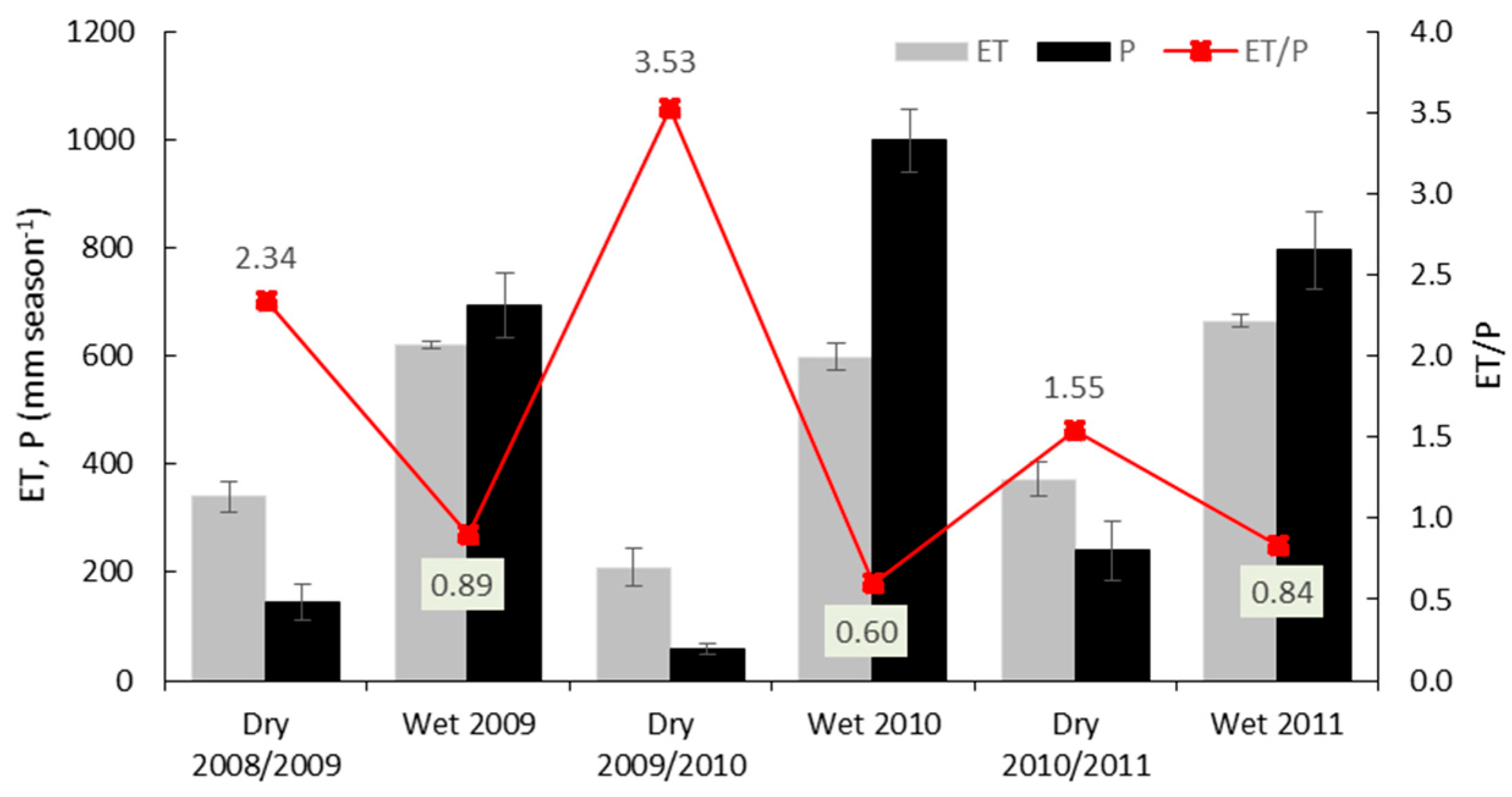
Ecosystem evapotranspiration (ET) varied significantly during these three years. The seasonal mean ET in the dry season was 208.8–372.0 mm and 598.5–664.7 mm in the wet season (Figure 6). During these three years, the average annual rainfall (P) was 798.5 mm and average ET was 743.7 mm. Thus, the annual ET/P ratios were 1.14, 0.79, and 1.04 in 2009, 2010, and 2011, respectively, while these were 1.5–3.5 in the dry season, and 0.6–0.9 in the wet season (Figure 6). Except for 2010, the ratios between ET/P were quite similar to those given by Kim et al. [38], who reported diverse land use in Tak (DTT) in Northern Thailand (average evaporation and rainfall during 2002–2013 was 1300 mm and 1230 mm, respectively). In 2010, despite the highest rainfall among these three years, evapotranspiration was the lowest.
The following may explain these inter−annual variations of evapotranspiration in relation to rainfall amount. During the year 2010 when extended drought occurred, it is generally recognized that a moderate El Niño occurred during the first half and a La Niña occurred during the second half of the year [28]. Thus, less rain than usual during the first half was compensated by more rain than usual during the second half of the year. This may have left the soil (during the first half of 2010) with a large water deficit and thus a higher capacity to absorb rainfall during the second half of the year. With relatively cooler air and soil temperatures, and lower VPD (as shown in Figure 2a,b), evaporation was relatively lower when compared to other years. A distinct difference in the evaporation rate between the dry and wet seasons corresponding to rainfall was a general characteristic of this site. The evapotranspiration rates during the daytime (7:00–18:00) dry season of 2008/2009, 2009/2010 and 2010/2011 were 3.60, 2.21 and 3.99 mm day−1 (average ± SD = 3.26 ± 0.94 mm day−1), respectively. During the wet season, these were 6.29, 6.10, and 6.81 mm day−1 (6.40 ± 0.37 mm day−1), respectively. These were much higher than those reported by Tanaka et al. [39], who reported values of 2–3 mm day−1 in the wet season and 1–3 mm day−1 in the dry season in a mature hill evergreen forest. Much higher evaporation rates of 5.6 and 5.9 mm day−1 during the dry season at an 8- and a 25-year-old secondary hill evergreen forest in northern Thailand were reported by Giambelluca et al. [11]. Since studies on the amount and seasonality of evapotranspiration in other secondary forests are still limited, more studies are required to know whether the relatively higher rate of evapotranspiration both in the dry and wet seasons is a common characteristic.
When the amount and rainfall and evaporation seasonally were considered, there were 1.5–2.3 times higher evapotranspiration than the amount of rainfall during the dry season, which was notably higher in the 2009/2010 dry season (3.5 times, Figure 6). In contrast, during the wet season, the amount of rainfall was 1.1–1.2 times higher than the amount of evaporation in 2009 and 2011, and was 1.7 times higher in wet season 2010. Thus, surplus rainfall during the wet season evaporated during the following dry season, which normally maintains the balance between rainfall and evaporation (e.g., in 2009 and 2011). Since it seems that water storage in the canopy and soil was limited due to the shallow soil profile and root depth (ca. 3 m) as mentioned above, this forest ecosystem relies on the limited input of water through rainfall during the wet season. During the dry season, the trees therefore shed their leaves to avoid damage from water stress. To understand the environmental controls of these seasonal and annual variations of ET, relationships between ET and micrometeorological variables were studied (unpublished). Our review found that the seasonal variations of ET were significantly related with rainfall (P), soil water content (SWC) and vapor pressure deficit (VPD). A positive correlation was observed between ET and P (R2 = 0.99, p < 0.01), ET and SWC (R2 = 0.96, p < 0.01), while a negative correlation was found between ET and VPD (R2 = 0.93, p < 0.01). Since soil water content is controlled mainly by rainfall, we concluded that both seasonal and inter-annual variations of ET were mainly controlled by the pattern of rainfall.
4. Conclusions
We investigated the energy fluxes and evapotranspiration in a secondary dry dipterocarp forest during 2008–2011 using the eddy covariance technique. Energy exchanges between this forest and the atmosphere were dominated by sensible heat fluxes during the dry and latent heat fluxes during the wet seasons. The annual energy balance closure was about 85–86% and varied between about 84–87% in the dry season, and 83–84% in the wet season. The energy balance closure in this secondary dry dipterocarp forest was in the lower range compared to that reported for other forest types. We discussed the potential sources of missing energy and suggested that storage in biomass and heterogeneity may partly contribute to the energy imbalance. On the other hand, the evaporation or the demand for evaporation in a secondary dry diperocarp forest was high throughout the year. Most of the annual rainfall in this forest was returned to the atmosphere through evapotranspiration, with an E/P ratio during these three years of 0.7–1.14. During the dry season, the E/P ratios were usually >1, and in the wet season, this was <1, indicating that partial rainfall was available in the dry season for evapotranspiration.
Acknowledgments
This study was supported by grants from the Science and Technology Postgraduate Education and Research Development Office (PERDO), and the National Research University Project of Thailand’s Office of the Higher Education Commission (CHE). We would like to acknowledge Monique Y. LeClerc from the Laboratory for Environmental Physics, Center of Atmospheric Biogeosciences, University of Georgia, Griffin, GA, USA, for helpful discussions during the beginning of this study period.
Author Contributions
All authors contributed to the research and field experimental design of this study and to the collaboration of this manuscript; Montri Sanwangsri performed the data collection and analysis, and prepared the first draft of this paper; Phonthep Hanpattanakit performed the data collection. Amnat Chidthaisong supervised the overall research work, provided guidelines for the write up of the manuscript, and contributed to its editing and finalization.
Conflicts of Interest
The authors declare no conflict of interest.
References
- Johnson, B.A. Combining national forest type maps with annual global tree cover maps to better understand forest change over time: Case study for Thailand. Appl. Geogr. 2015, 62, 294–300. [Google Scholar] [CrossRef]
- Leinenkugel, P.; Wolters, M.L.; Oppelt, N.; Kuenzer, C. Tree cover and forest cover dynamics in the Mekong Basin from 2001 to 2011. Remote Sens. Environ. 2015, 158, 376–392. [Google Scholar] [CrossRef]
- Flint, E.P. Changes in land use in South and Southeast Asia from 1880 to 1980: A data base prepared as part of a coordinated research program on carbon fluxes in the tropics. Chemosphere 1994, 29, 1015–1062. [Google Scholar] [CrossRef]
- Wright, S.J. Tropical forests in a changing environment. Trends Ecol. Evol. 2005, 20, 553–560. [Google Scholar] [CrossRef] [PubMed]
- Fukushima, M.; Kanzaki, M.; Hara, M.; Ohkubo, T.; Preechapanya, P.; Choocharoen, C. Secondary forest succession after the cessation of swidden cultivation in the montane forest area in Northern Thailand. For. Ecol. Manag. 2008, 255, 1994–2006. [Google Scholar] [CrossRef]
- Brown, S.; Lugo, A.E. Tropical secondary forests. J. Trop. Ecol. 1990, 6, 1–32. [Google Scholar] [CrossRef]
- Bonner, M.T.L.; Schmidt, S.; Shoo, L.P. A meta-analytical global comparison of aboveground biomass accumulation between tropical secondary forests and monoculture plantations. For. Ecol. Manag. 2013, 291, 73–86. [Google Scholar] [CrossRef]
- International Tropical Timber Organization. ITTO Guidelines for the Restoration, Management and Rehabilitation of Degraded and Secondary Tropical Forests; International Tropical Timber Organization: Yokohama, Japan, 2002; p. 86. [Google Scholar]
- Food and Agriculture Organization of the United Nations. Global Forest Resources Assessment 2015, Desk Reference; Food and Agriculture Organization of the United Nations: Rome, Italy, 2015; p. 253. Available online: http://www.fao.org/3/a-i4808e.pdf (accessed on 16 July 2016).
- Sommer, R.; Abreu Sa, T.D.; Vielhauer, K.; Araújo, A.C.; Fölster, H.; Vlek, P.L.G. Transpiration and canopy conductance of secondary vegetation in the eastern Amazon. Agric. For. Meteorol. 2002, 112, 103–121. [Google Scholar] [CrossRef]
- Giambelluca, T.W.; Nullet, M.A.; Ziegler, A.D.; Tran, L. Latent and sensible energy flux over deforested land surfaces in the eastern Amazon and northern Thailand. Singap. J. Trop. Geogr. 2000, 21, 107–130. [Google Scholar] [CrossRef]
- Tanaka, N.; Kume, T.; Yoshifuji, N.; Tanaka, K.; Takizawa, H.; Shiraki, K.; Tantasirin, C.; Tangtham, N.; Suzuki, M. A review of evapotranspiration estimates from tropical forest in Thailand and adjacent regions. Agric. For. Meteorol. 2008, 148, 807–819. [Google Scholar] [CrossRef]
- Toda, M.; Nishida, K.; Ohte, N.; Tani, M.; Mushiake, K. Observations of energy fluxes and evapotranspiration over terrestrial complex land covers in the tropical monsoon environment. J. Meteorol. Soc. Jpn. 2002, 80, 465–484. [Google Scholar] [CrossRef]
- Phianchroen, M.; Duangphakdee, O.; Chanchae, P. Instruction of Plant in Dry Dipterocarp Forest at King Mongkut’s University of Technology Thonburi at Ratchaburi Campus; King Mongkut’s University of Technology Thonburi press: Bangkok, Thailand, 2008; p. 170. (In Thai) [Google Scholar]
- Arya, S.P. Introduction to Micrometeorology, 2nd ed.; Academic Press: Cambridge, MA, USA, 1988; p. 307. [Google Scholar]
- Stull, R.B. An Introduction to Boundary Layer Meteorology; Kluwer Academic Publishers: Dordrecht, The Netherlands, 1998; p. 670. [Google Scholar]
- Hanpattanakit, P.; Leclerc, M.Y.; Mcmillan, A.M.S.; Limtong, P.; Maeght, J.L.; Panuthai, S.; Inubushi, K.; Chidthaisong, A. Multiple timescale variations and controls of soil respiration in a tropical dry dipterocarp forest, western Thailand. Plant Soil 2015, 390, 167–181. [Google Scholar] [CrossRef]
- Kaimal, J.C.; Finnigan, J.J. Atmospheric Boundary Layer Flow: Their Structure and Measurement; Oxford University Press: New York, NY, USA, 1994; p. 289. [Google Scholar]
- Bonan, G.B. Ecological Climatology: Concepts and Applications; Cambridge University Press: Cambridge, UK, 2002; p. 678. [Google Scholar]
- Foken, T. Micrometeorology; Springer: Berlin/Heidelberg, Germany, 2008; p. 308. [Google Scholar]
- Oliphant, A.J.; Grimmond, C.S.B.; Zutter, H.N.; Schmid, H.P.; Su, H.B.; Scott, S.L.; Offer, B.; Randolph, J.C.; Ehman, J. Heat storage and energy balance fluxes for a temperate deciduous forest. Agric. For. Meteorol. 2004, 126, 185–201. [Google Scholar] [CrossRef]
- Sánchez, J.M.; Caselles, V.; Rubio, E.M. Analysis of the energy balance closure over a FLUXNET boreal forest in Finland. Hydrol. Earth Syst. Sci. 2010, 14, 1487–1497. [Google Scholar] [CrossRef]
- Vickers, D.; Mahrt, L. Quality control and flux sampling problems for tower and aircraft data. J. Atmos. Ocean Technol. 1997, 14, 512–526. [Google Scholar] [CrossRef]
- Vickers, D.; Thomas, C.; Law, B.E. Random and systematic CO2 flux sampling errors for tower measurements over forests in the convective boundary layer. Agric. For. Meteorol. 2009, 149, 73–83. [Google Scholar] [CrossRef]
- Webb, E.K.; Pearman, G.I.; Leuning, R. Correction of flux measurements for density effects due to heat and water vapor transfer. Q. J. R. Meteorol. Soc. 1980, 106, 85–100. [Google Scholar] [CrossRef]
- Moncrieff, J.; Clement, R.; Finnigan, J.; Meyers, T. Averaging, detrending, and filtering of eddy covariance time series. In Handbook of Micrometeorology: A Guide for Surface Flux Measurements; Lee, X., Massman, W.J., Law, B.E., Eds.; Kluwer Academic Publishers: Dordrecht, The Netherlands, 2004; pp. 7–31. [Google Scholar]
- Wolf, S.; Eugster, W.; Potvin, C.; Buchmann, N. Strong seasonal variations in net ecosystem CO2 exchange of a tropical pasture and afforestation in Panama. Agric. For. Meteorol. 2011, 151, 1139–1151. [Google Scholar] [CrossRef]
- Barnard, P.L.; Allan, J.; Hansen, J.E.; Kaminsky, G.M.; Ruggiero, P.; Doria, A. The impact of the 2009–10 El Niño Modoki on U.S. West Coast beaches. Geophys. Res. Lett. 2011, 38, 13604. [Google Scholar] [CrossRef]
- Rosenberg, N.J.; Blad, B.L.; Verma, S.B. Microclimate: The Biological Environment, 2nd ed.; John Wiley and Sons: New York, NY, USA, 1983; p. 495. [Google Scholar]
- Henry, J.G.; Heinke, G.W. Environmental Science and Engineering, 2nd ed.; Prentice-Hall International, Inc.: London, UK, 1996; p. 778. [Google Scholar]
- Hirai, K.; Tanaka, H.; Suksawang., S. Albedo characteristics of mixed deciduous forest and teak plantation in Thailand. Proceeding of the International Conference on Tropical Forest and Climate Change: Status, Issues and Challenges (TFCC’98), Makati, Philippines, 19–22 October 1998. [Google Scholar]
- Stoy, P.C.; Mauder, M.; Foken, T.; Marcolla, B.; Boegh, E.; Ibrom, A.; Arain, M.A.; Arneth, A.; Aurela, M.; Bernhofer, C.; et al. A data-driven analysis of energy balance closure across FLUXNET research site: The role of landscape scale heterogeneity. Agric. For. Meteorol. 2013, 152, 137–152. [Google Scholar] [CrossRef]
- Wilson, K.; Goldstein, A.; Falge, E.; Aubinet, M.; Baldocchi, D.; Berbigier, P.; Bernhofer, C.; Ceulemans, R.; Dolman, H.; Field, C.; et al. Energy balance closure at FLUXNET site. Agric. For. Meteorol. 2002, 133, 233–243. [Google Scholar] [CrossRef]
- Foken, T.; Wimmer, F.; Mauder, M.; Thomas, C.; Liebethal, C. Some aspects of the energy balance closure problem. Atmos. Chem. Phys. 2006, 6, 4395–4402. [Google Scholar] [CrossRef]
- Cava, A.D.; Contini, D.; Donateo, A.; Martano, P. Analysis of short-term closure of the surface energy balance above short vegetation. Agric. For. Meteorol. 2008, 148, 82–93. [Google Scholar] [CrossRef]
- Lindroth, A.; Molder, M.; Lagergren, F. Heat storage in forest biomass improves energy balance closure. Biogeosciences 2010, 7, 301–313. [Google Scholar] [CrossRef]
- Da Rocha, H.R.; Goulden, M.L.; Miller, S.D.; Menton, M.C.; Pinto, L.; Freitas, H.C.; Figueira, A.M.S. Seasonality of water and heat fluxes over a tropical forest in eastern Amazonia. Ecol. Appl. 2004, 14, 22–32. [Google Scholar] [CrossRef]
- Kim, W.; Komori, D.; Cho, J.; Kanae, S.; Oki, T. Long-term analysis of evapotranspiration over a diverse land use area in northern Thailand. Hydrol. Res. Lett. 2014, 8, 45–50. [Google Scholar] [CrossRef]
- Tanaka, K.; Kosugi, Y.; Nakamura, A. Impact of leaf physiological characteristics on seasonal variation in CO2, latent and sensible heat exchanges over a tree plantation. Agric. For. Meteorol. 2002, 114, 103–122. [Google Scholar] [CrossRef]
Figure 1.
Satellite image illustrating dry dipterocarp forest flux site at the Ratchaburi site Thailand (DFR), located at 13°35′13.3′′ N, 99°30′3.9′′ E. The inner white circle indicates minimum and maximum fetch in a north-south direction (500 m), and the outer white cycle indicates fetch in an east-west direction (1200 m) within the forest area. The wind rose and main wind direction were northwest towards the southeast (mean wind speed 1.15 m s−1). The typical wind speed ranged between 0.95 and 1.49 m s−1 (measured at 8 m height from the soil surface).
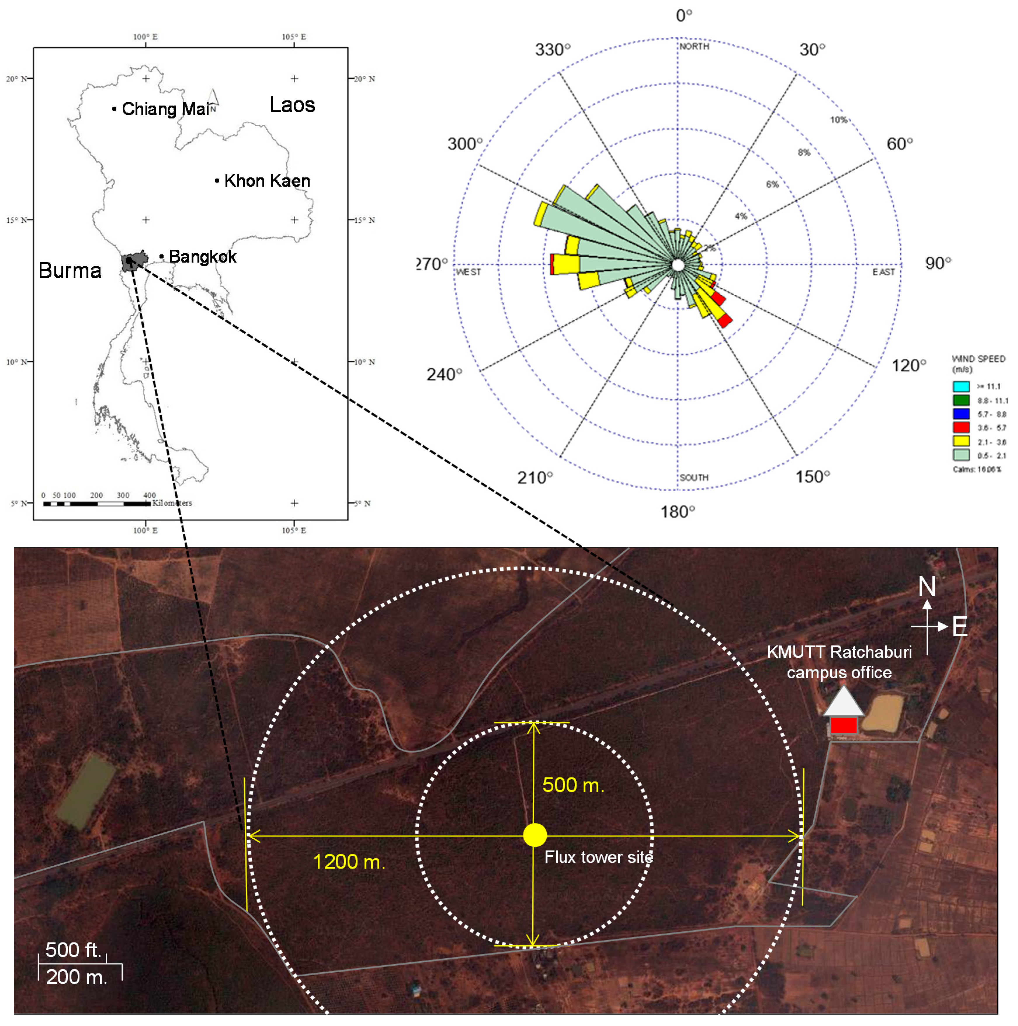
Figure 2.
(a) Daily cumulative rainfall (solid bar in unit of mm), daily mean soil water content (cross symbol right y-axis in % volumetric water content), daily mean soil temperature (open circle,) at 5 cm depth, and daily mean air temperature (red triangle) during the study period. The horizontal solid line demarks soil water content (SWC) at 5% volumetric water content (VWC); (b) Variations of daily vapor pressure deficit (VPD); and (c) Daily pattern of net radiation (Rn, open circle), sensible heat flux (H, open triangle), latent heat flux (LE, plus symbol) and soil heat flux at 8 cm depth (Gs, cross symbol). The vertical dashed lines indicate the separation of dry (November–April) and wet seasons (May–October).
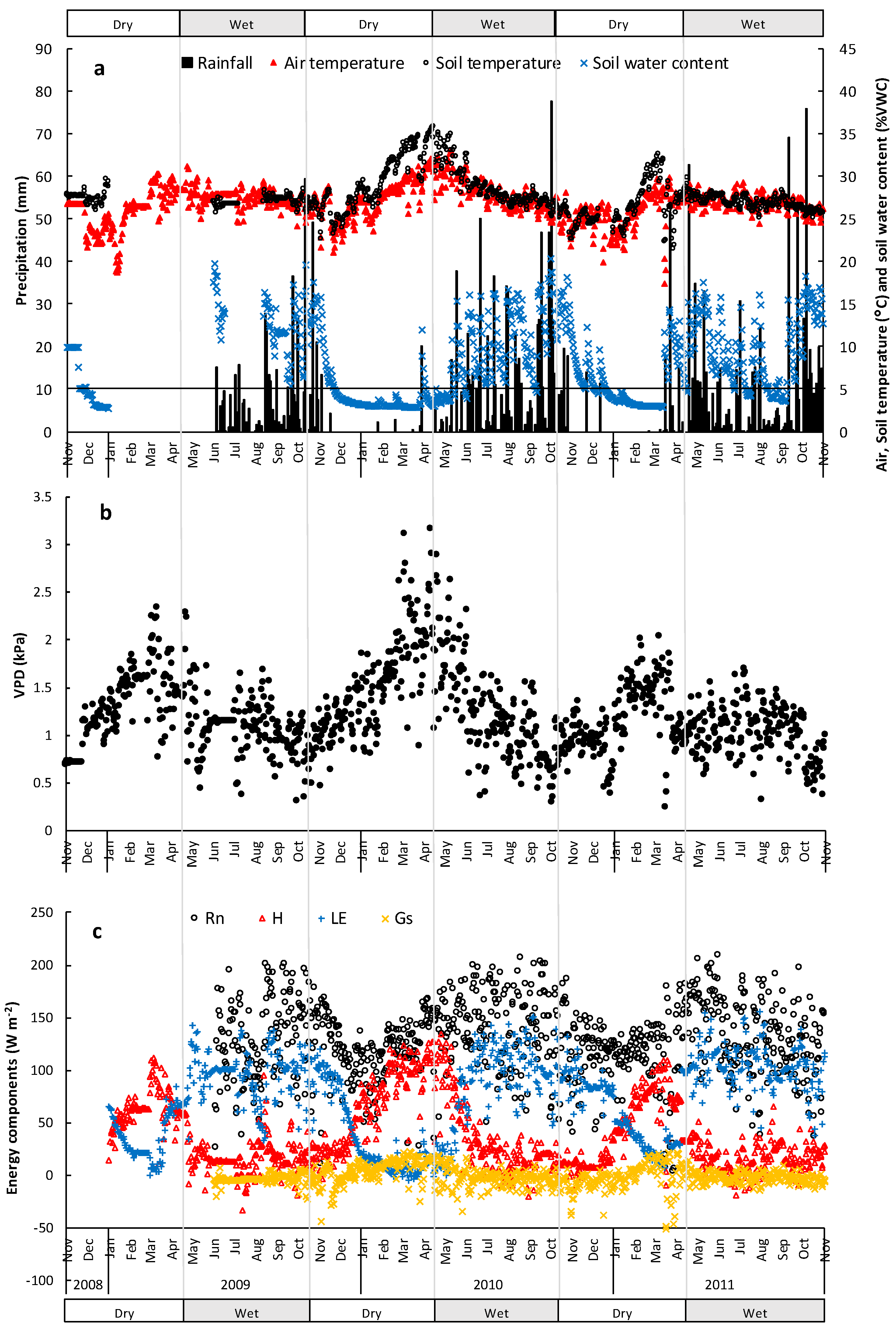
Figure 3.
Average diurnal variations of energy components (W m−2); net radiation (Rn, solid line), sensible heat flux (H, heavy dashed line), latent heat flux (LE, dot line) and soil heat flux at 8 cm depth (Gs, long dashed line) for the dry season (a) and wet season (b) in the secondary dry dipterocarp forest site.
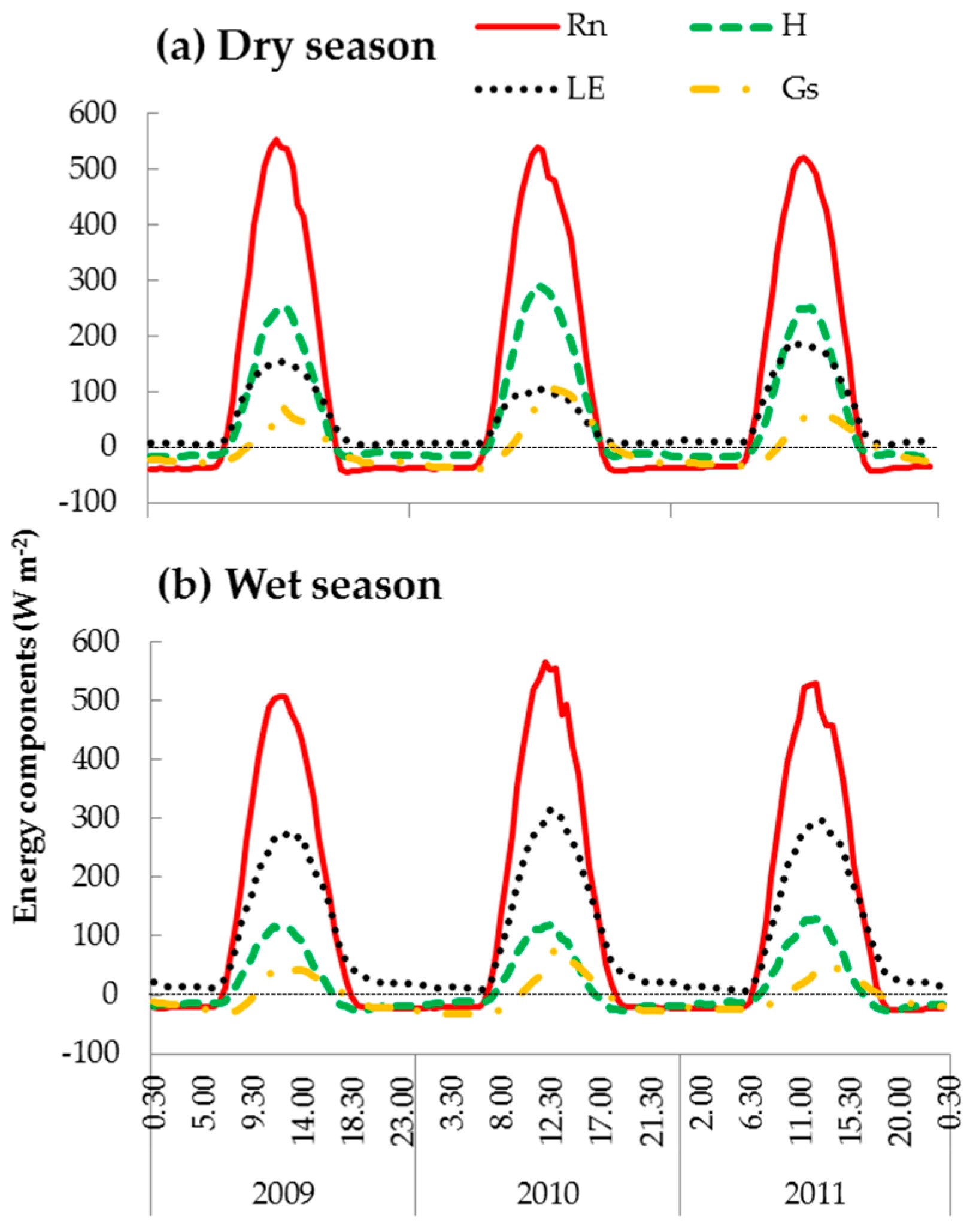
Figure 4.
Annual energy balance closure in 2010 (a) n = 17,520; and 2011 (b) n = 17,520 and seasonal energy balance closure for the dry season (c) n = 20,304; and wet season (d) n = 17,661 at a secondary dry dipterocarp forest site. The round dotted line denotes the ideal closure (1:1). Linear regressions are strongly significant (p < 0.001) for the whole year.
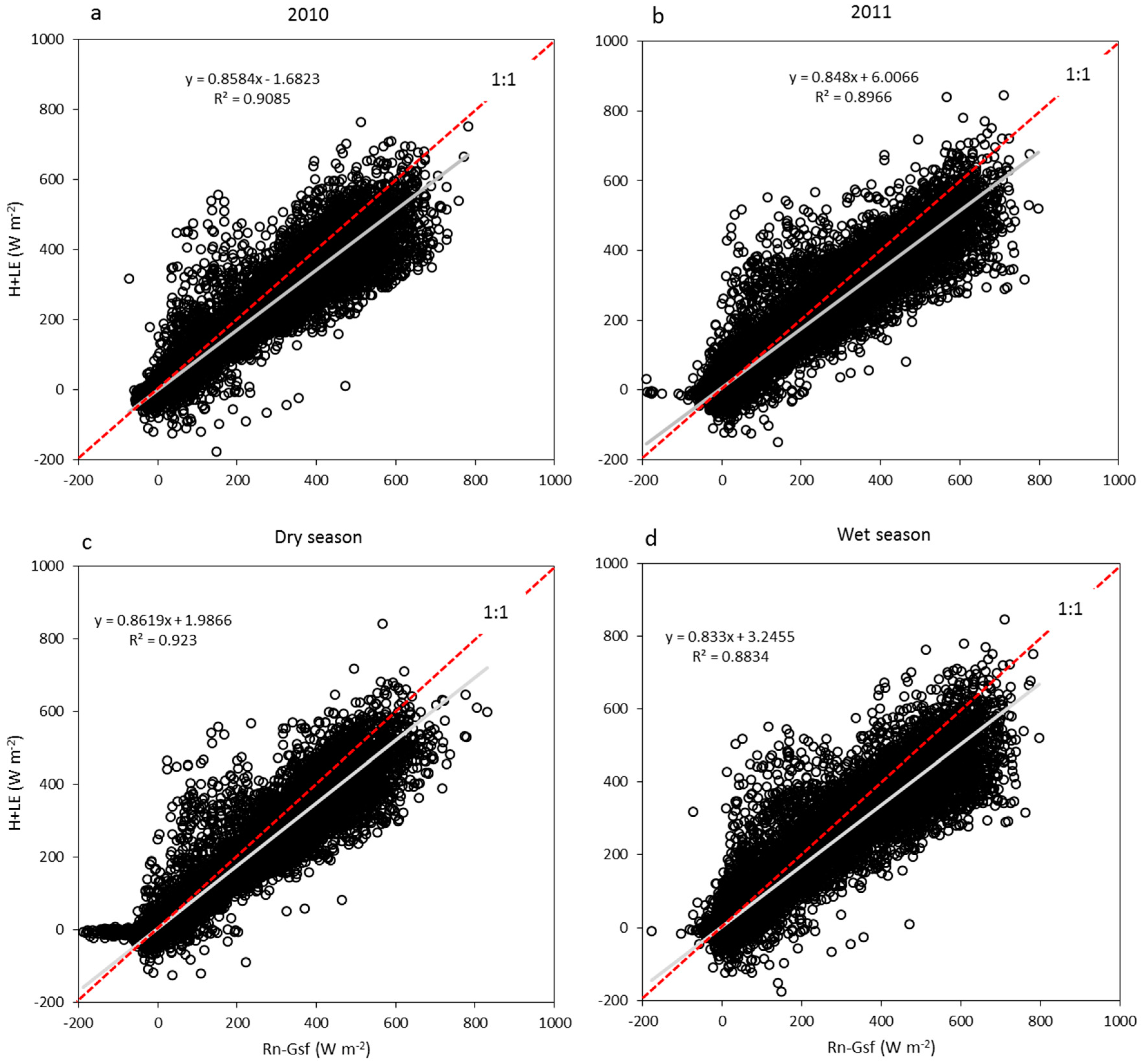
Figure 5.
Comparison between the average diurnal variation of residual energy (Re) computed using the uncorrected (Rn-H-LE-Gs) and that corrected with heat storage in the soil column (Rn-H-LE-Gs-ΔG). The cross line represents net radiation (Rn) in the dry dipterocarp forest during November 2009 to October 2011. Note that the dry season is from November to April, and the wet season is from May to October.
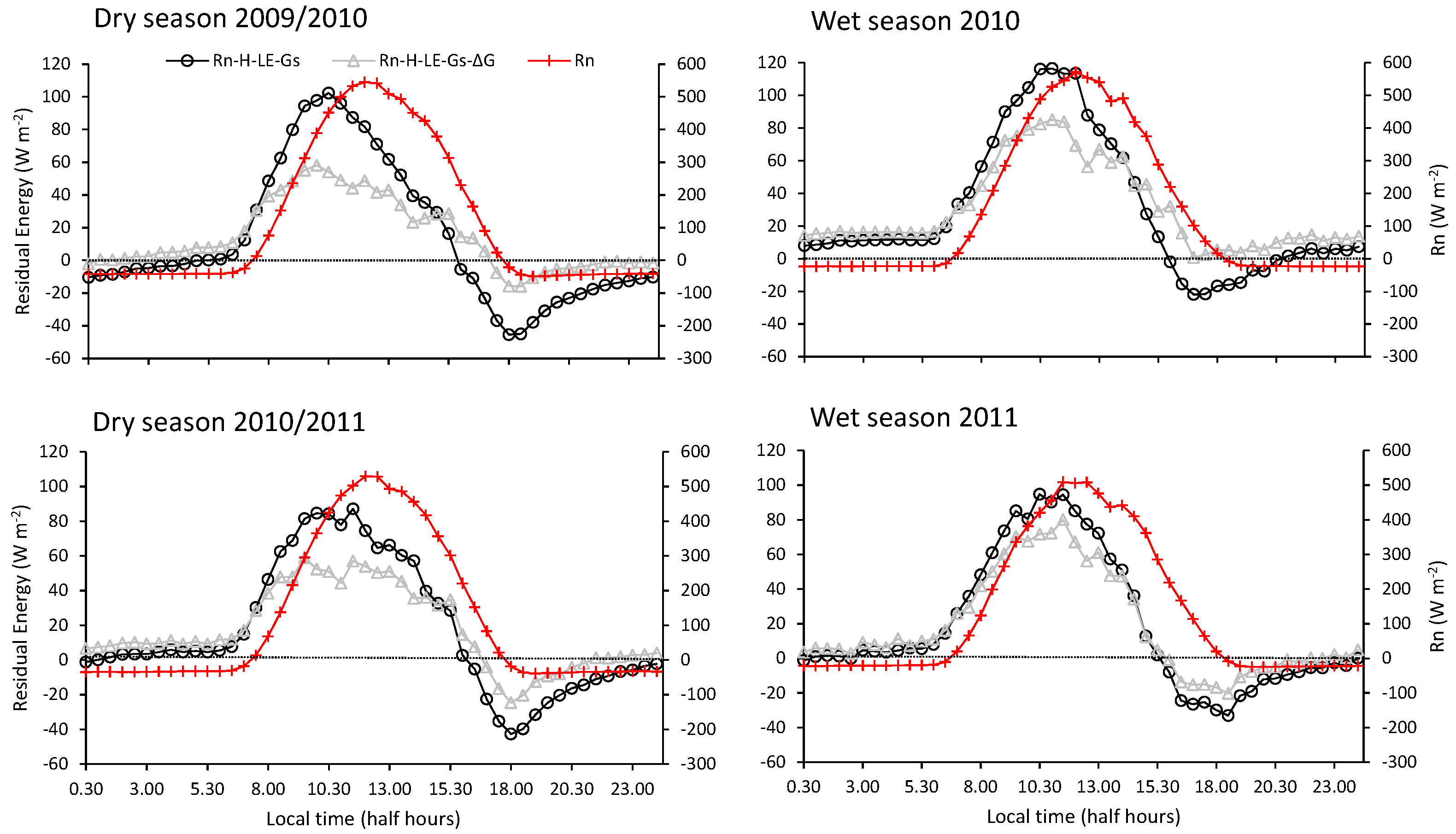
Figure 6.
Seasonal means of ecosystem evapotranspiration (ET), precipitation (P) and the ratios ET/P observed at DFR site in dry season 2008/2009 until the wet season in 2011, including error bars.
Figure 6.
Seasonal means of ecosystem evapotranspiration (ET), precipitation (P) and the ratios ET/P observed at DFR site in dry season 2008/2009 until the wet season in 2011, including error bars.

Table 1.
Seasonal and monthly energy budget and its components in the young secondary dry dipterocarp forest.
Table 1.
Seasonal and monthly energy budget and its components in the young secondary dry dipterocarp forest.
| Seasonality | Monthly | Rn | H | LE | Gsf | Albedo | Rn | H | LE | Gsf |
|---|---|---|---|---|---|---|---|---|---|---|
| (W m−2) | (%) | |||||||||
| Wet season 2009 | May | * | * | * | * | * | * | * | * | * |
| Jun | 122.71 | 13.52 | 100.49 | −5.30 | 0.17 | 100 | 11 | 82 | −4 | |
| Jul | 110.66 | 4.01 | 96.55 | −4.48 | 0.17 | 100 | 4 | 87 | −4 | |
| Aug | 132.47 | 30.72 | 83.42 | −3.75 | 0.17 | 100 | 23 | 63 | −3 | |
| Sep | 142.77 | 15.80 | 99.82 | −2.33 | 0.16 | 100 | 11 | 70 | −2 | |
| Oct | 140.12 | 19.15 | 94.76 | −3.53 | 0.15 | 100 | 14 | 68 | −3 | |
| average | 129.75 | 16.64 | 95.01 | −3.88 | 0.16 | 100 | 13 | 74 | −3 | |
| SE | 13.21 | 9.67 | 6.89 | 1.11 | 0.01 | |||||
| Dry season 2009/2010 | Nov | 131.62 | 19.67 | 93.55 | −6.27 | 0.15 | 100 | 15 | 71 | −5 |
| Dec | 106.50 | 41.12 | 48.11 | 2.01 | 0.16 | 100 | 39 | 45 | 2 | |
| Jan | 96.33 | 67.69 | 14.50 | 3.66 | 0.17 | 100 | 70 | 15 | 4 | |
| Feb | 120.42 | 94.56 | 7.04 | 11.32 | 0.17 | 100 | 79 | 6 | 9 | |
| Mar | 118.35 | 96.41 | 6.05 | 10.91 | 0.18 | 100 | 81 | 5 | 9 | |
| Apr | 144.20 | 106.97 | 15.47 | 8.15 | 0.17 | 100 | 74 | 11 | 6 | |
| average | 119.57 | 71.07 | 30.79 | 4.96 | 0.17 | 100 | 60 | 25 | 4 | |
| SE | 17.12 | 34.74 | 34.39 | 6.67 | 0.01 | |||||
| Wet season 2010 | May | 142.73 | 74.98 | 46.23 | −0.18 | 0.16 | 100 | 53 | 32 | 0 |
| Jun | 150.98 | 31.04 | 102.35 | −2.37 | 0.17 | 100 | 21 | 68 | −2 | |
| Jul | 143.83 | 15.30 | 108.01 | −3.82 | 0.17 | 100 | 11 | 75 | −3 | |
| Aug | 131.65 | 9.88 | 104.97 | −4.86 | 0.17 | 100 | 8 | 80 | −4 | |
| Sep | 156.80 | 17.64 | 102.58 | −2.16 | 0.16 | 100 | 11 | 65 | −1 | |
| Oct | 121.08 | 11.10 | 92.48 | −9.18 | 0.15 | 100 | 9 | 76 | −8 | |
| average | 141.18 | 26.66 | 92.77 | −3.76 | 0.16 | 100 | 19 | 66 | −3 | |
| SE | 13.00 | 24.85 | 23.39 | 3.09 | 0.01 | |||||
| Dry season 2010/2011 | Nov | 115.86 | 6.29 | 87.77 | −7.55 | 0.15 | 100 | 5 | 76 | −7 |
| Dec | 113.10 | 15.74 | 81.93 | −6.48 | 0.15 | 100 | 14 | 72 | −6 | |
| Jan | 114.45 | 50.36 | 77.76 | −2.32 | 0.16 | 100 | 44 | 68 | −2 | |
| Feb | 119.32 | 78.96 | 27.02 | 9.13 | 0.16 | 100 | 66 | 23 | 8 | |
| Mar | 93.91 | 75.62 | 22.66 | −2.16 | 0.16 | 100 | 81 | 24 | −2 | |
| Apr | 150.65 | 41.91 | 84.35 | 4.24 | 0.15 | 100 | 28 | 56 | 3 | |
| average | 117.88 | 44.81 | 63.58 | −0.86 | 0.15 | 100 | 40 | 53 | −1 | |
| SE | 18.38 | 29.94 | 30.22 | 6.42 | 0.01 | |||||
| Wet season 2011 | May | 163.37 | 20.41 | 114.58 | −1.26 | 0.15 | 100 | 12 | 70 | −1 |
| Jun | 125.02 | 3.24 | 101.79 | −2.63 | 0.16 | 100 | 3 | 81 | −2 | |
| Jul | 128.42 | 12.33 | 113.48 | −3.01 | 0.16 | 100 | 10 | 88 | −2 | |
| Aug | 132.23 | 23.78 | 98.69 | −0.86 | 0.16 | 100 | 18 | 75 | −1 | |
| Sep | 121.43 | 12.81 | 106.40 | −2.04 | 0.15 | 100 | 11 | 88 | −2 | |
| Oct | 112.20 | 18.71 | 84.85 | −5.12 | 0.15 | 100 | 17 | 76 | −5 | |
| average | 130.45 | 15.21 | 103.30 | −2.49 | 0.16 | 100 | 12 | 80 | −2 | |
| SE | 17.52 | 7.35 | 10.99 | 1.52 | 0.01 | |||||
| Total dry | 118.73 | 57.94 | 47.18 | 2.05 | 0.16 | 100 | 50 | 39 | 2 | |
| Total wet | 144.76 | 21.24 | 100.79 | −2.97 | 0.16 | 100 | 14 | 73 | −3 | |
| Total all season | 131.75 | 39.59 | 73.99 | −0.46 | 0.16 | 100 | 32 | 56 | −1 | |
Note: Net radiation (Rn), sensible heat flux (H), latent heat flux (LE) at 8 m height and soil heat flux at the surface (Gsf); negative data represent heat loss from the soil; * data not available.
© 2017 by the authors. Licensee MDPI, Basel, Switzerland. This article is an open access article distributed under the terms and conditions of the Creative Commons Attribution (CC BY) license (http://creativecommons.org/licenses/by/4.0/).
Share and Cite
MDPI and ACS Style
Sanwangsri, M.; Hanpattanakit, P.; Chidthaisong, A. Variations of Energy Fluxes and Ecosystem Evapotranspiration in a Young Secondary Dry Dipterocarp Forest in Western Thailand. Atmosphere 2017, 8, 152. https://doi.org/10.3390/atmos8080152
AMA Style
Sanwangsri M, Hanpattanakit P, Chidthaisong A. Variations of Energy Fluxes and Ecosystem Evapotranspiration in a Young Secondary Dry Dipterocarp Forest in Western Thailand. Atmosphere. 2017; 8(8):152. https://doi.org/10.3390/atmos8080152
Chicago/Turabian StyleSanwangsri, Montri, Phongthep Hanpattanakit, and Amnat Chidthaisong. 2017. "Variations of Energy Fluxes and Ecosystem Evapotranspiration in a Young Secondary Dry Dipterocarp Forest in Western Thailand" Atmosphere 8, no. 8: 152. https://doi.org/10.3390/atmos8080152
Note that from the first issue of 2016, this journal uses article numbers instead of page numbers. See further details here.