Data Assimilation in Air Contaminant Dispersion Using a Particle Filter and Expectation-Maximization Algorithm


College of Information System and Management, National University of Defense Technology, 109 Deya Road, Changsha 410073, China
*
Author to whom correspondence should be addressed.
Atmosphere 2017, 8(9), 170; https://doi.org/10.3390/atmos8090170
Submission received: 27 July 2017
/
Revised: 6 September 2017
/
Accepted: 8 September 2017
/
Published: 16 September 2017
(This article belongs to the Section Air Quality)
Abstract
:The accurate prediction of air contaminant dispersion is essential to air quality monitoring and the emergency management of contaminant gas leakage incidents in chemical industry parks. Conventional atmospheric dispersion models can seldom give accurate predictions due to inaccurate input parameters. In order to improve the prediction accuracy of dispersion models, two data assimilation methods (i.e., the typical particle filter & the combination of a particle filter and expectation-maximization algorithm) are proposed to assimilate the virtual Unmanned Aerial Vehicle (UAV) observations with measurement error into the atmospheric dispersion model. Two emission cases with different dimensions of state parameters are considered. To test the performances of the proposed methods, two numerical experiments corresponding to the two emission cases are designed and implemented. The results show that the particle filter can effectively estimate the model parameters and improve the accuracy of model predictions when the dimension of state parameters is relatively low. In contrast, when the dimension of state parameters becomes higher, the method of particle filter combining the expectation-maximization algorithm performs better in terms of the parameter estimation accuracy. Therefore, the proposed data assimilation methods are able to effectively support air quality monitoring and emergency management in chemical industry parks.
1. Introduction
Air contaminant emissions and contaminant gas leakage incidents in chemical industry parks are significant events, which can pose a potential threat to public health. Therefore, understanding the dispersion of air contaminants is essential to air quality monitoring and emergency responses to gas leakage incidents. Most conventional methods of predicting atmospheric dispersion rely on the atmospheric dispersion models (e.g., the Gaussian models and Lagrangian models) with some given input model parameters. However, due to the dynamic and stochastic nature of atmospheric dispersion, it is impractical to measure these model parameters precisely, especially the meteorological data (e.g., the wind field). Further, the source term (i.e., source location and release rate) is often unknown. These inaccurate or unknown parameters result in the inaccurate model prediction of air contaminant dispersion.
Data assimilation (DA) provides an approach of dynamically estimating model parameters and effectively improving the accuracy of model predictions. This approach assimilates the observations into the model to produce a time sequence of estimates of system states [1]. In order to deal with the imperfect model parameters, the data assimilation tries to find the solutions of parameter estimations by minimizing the errors between the real system and the models [2]. With the model parameters adjusted, the accuracy of the model prediction is consequently improved. Therefore, data assimilation has been widely used in various fields, especially in numerical weather forecasting, meteorological pre-processing, and wild fire spreading [2,3], which all demand the high accuracy of prediction. Common methods of data assimilation include the variational approach [4], Kalman filter [5] and its variants (e.g., extended Kalman filter [6] and Ensemble Kalman filter [7]), and particle filter [8,9]. Among these methods, particle filter is one of the most suitable approaches for highly nonlinear and non-Gaussian models. Using a series of weighted random sampling particles to approximate the posterior probability density function of the system state, particle filter is able to estimate arbitrary probability densities with few assumption constraints. Therefore, particle filter is applied as the data assimilation method in the air contaminant dispersion in this paper. As for the air contaminant emission, we focus on two cases in the chemical plants. One is the daily emission occurring every day, in which the source term is known in advance because the emission is under the control of the chemical plant. The other one is the contaminant gas leakage incident, in which the release rate is hard to measure for the sake of safety. Additionally, the variation in the release rate also increases the difficulty of measuring the source term. In the contaminant gas leakage incident, with the release rate to be estimated, the accuracy of particle filter might decrease due to the higher dimension of the state vector. To deal with this problem, the particle filter is combined with the expectation-maximization (EM) algorithm [10]. The EM algorithm is a parameter estimation method for the incomplete-data problem, which divides the estimation of complex parameters into iterations with two steps (i.e., the Expectation Step (E-step) and the Maximization Step (M-step)). Further, the EM algorithm is applied to improve the performance of parameter estimations [11] in some fields, such as in target tracking [12].
Data assimilation needs the observed data of air contaminants. In chemical industry parks, the conventional way of obtaining these observations mainly depends on the static ground monitoring station. Although the station has a high detecting accuracy, its fixed location limits the area of data collection, especially when the station is located in the upwind of the emission source. Fortunately, the emergence of Unmanned Aerial Vehicles (UAV) has initialed a revolution in this research. Providing flexible mobility in space, the UAV becomes an efficient tool of data collection in atmospheric environment monitoring. Yang and Huang [13] utilized a sensory system based on an unmanned helicopter to monitor the , , and in a chemical industry park. The UAV has also been used in the source term estimation and boundary tracking of atmospheric dispersion [14,15].
In this paper, the Gaussian plume model is applied to describe the air contaminant dispersion. In order to improve the accuracy of model predictions, data assimilation based on particle filter is utilized to assimilate the observations into the atmospheric dispersion model in the two emission cases. The observation is collected by the virtual UAV in numerical experiments instead of the field experiment. In the first case, four coefficients of dispersion in the Gaussian plume model are selected as the state parameters to be estimated. In the second case, the release rate is added into the state parameters. Further, to deal with the high dimension of state parameters in the second case, the particle filter is combined with the EM algorithm. The performances of particle filter and the method of particle filter combining the EM algorithm are tested by two numerical experiments. This paper is the starting point of the work of data assimilation in air contaminant dispersion because the Gaussian plume model and virtual observations used in this paper are different from the real situation. The rest of this paper is organized as follows. Section 2 introduces the atmospheric dispersion model and data assimilation methods using typical particle filter and particle filter combining the EM algorithm. Section 3 describes the numerical experiments. An analysis of the results is given in Section 4. Discussions and conclusions are made in Section 5 and Section 6, respectively.
2. Model and Methods
2.1. Atmospheric Dispersion Model
The modeling of air contaminant dispersion is the basis of the dispersion prediction. The Gaussian models are widely used in atmospheric dispersion. Requiring only a few input parameters, Gaussian models are simpler compared to some complex models like the Lagrangian model. Further, the results of Gaussian models are trustworthy for near-field dispersion cases. Consequently, the Gaussian models are suitable for the modeling of air contaminant dispersion in data assimilation, which requires fast computing of the dispersion model. In this paper, the Gaussian plume model is applied to model the continuous release of the point source in the chemical industry park. In this model, the air contaminant concentration of a given point (x, y, z) is expressed as follows:
where x, y, and z are the coordinates of downwind, crosswind, and vertical directions, respectively. Parameter of u is the wind velocity. He and q represent the effective height and release rate of the source, respectively. The effective height of the source (He) is calculated by: , where H and Δh represent the physical height of the source and the height of plume rise. The plume rise height () is calculated by the formula in CALPUFF [16]. The plume rise due to buoyancy and momentum during neutral or unstable conditions is:
where is the momentum flux (), F is the buoyancy flux (), is the source height wind speed (), is the downwind distance (), is the neutral entrainment parameter, is the jet entrainment coefficient (), and w is the source gas exit speed (m/s). In addition, considering the deposition velocity , Equation (1) is rewritten as:
In the Gaussian plume model, the air contaminant concentration in axis y and z is considered to follow the Gaussian distribution. Therefore, the key parameters of the model are and , which represent the standard deviations that describe the crosswind and vertical mixing of air contaminants. The standard deviations can be described by empirical formulas:
where x represents the downwind distance. The parameters of a, b, c, and d are dispersion coefficients closely related to the environmental conditions, such as atmospheric stability and terrain. Several derivations of these dispersion coefficients exist where a popular approach is based on the Pasquill’s atmospheric stability class [17]. The empirical formulas of and illustrate that the standard deviations increase with the downwind distance. The Gaussian plume model can be applied to model the continuous release of the point source in the chemical industry park. However, relying solely on this model may fail to make an accurate prediction, since these model parameters usually vary with the environmental conditions and are hard to measure precisely. For example, we can only obtain their empirical values of the four dispersion coefficients, but no accurate value is available. There is currently no perfect formula to calculate these coefficients from the atmospheric stability. As for the wind field parameters (i.e., wind direction and velocity), they are also difficult to precisely measure. Further, the release rate q is usually unknown during the contaminant gas leakage incident. Without accurate parameters in the conventional modeling of atmospheric dispersion, it is a common practice to bring imperfect estimations of these parameters into the model for calculation, which inevitably introduces errors into the model prediction. Thus, there is an urgent need to dynamically estimate these parameters to improve the accuracy of the model prediction.
2.2. Data Assimilation Using Particle Filter
For the modeling of air contaminant dispersion, in order to diminish the errors of input parameters and produce an accurate prediction, a data assimilation model based on particle filter is developed. Particle filter, also called the Sequential Monte Carlo (SMC) method, is a sample-based method that uses Bayesian inference and stochastic sampling techniques to recursively estimate the state of the dynamic system from some given observations. The core idea of particle filter is using a series of weighted random sampling particles to approximate the posterior probability density function of the system state. A typical particle filter algorithm includes four steps (i.e., initialization, importance sampling, weight update, and resample) and goes through multiple iterations. In order to apply particle filter to the Gaussian plume model, the state space model of atmospheric dispersion needs to be developed. Usually, a dynamic system can be described and formulated as a discrete state space model:
where (6) and (7) represent the system state transition model and measurement model, respectively. and are system state variables and measurement variables at time step t, respectively. The function f describes the transition of the system states with time. The function g defines the relationship between state variables and measurement variables. The parameters of and are two independent random variables representing the state noise and the measurement noise, respectively.
The state transition model is based on the state parameters. Therefore, the selection of the state parameters is key to the construction of the state transition model. For the Gaussian plume model, there are several choices of state parameters. One of the common practices is dividing the area of dispersion into numerous grids and choosing the concentrations by grid as the state parameters. This choice directly describes the atmospheric dispersion. However, the vast region of the chemical industry park means a high dimension of the state parameters, which results in a high computation cost. In this paper, the dispersion coefficients a, b, c, and d in (4) and (5), as well as the release rate q, are selected as the state parameters in the second case, while the state parameters in the first case only include four dispersion coefficients. Selected as the state parameters, the four dispersion coefficients play important roles in the Gaussian plume model. The standard deviations and , which are derived from the four dispersion coefficients, describe the crosswind and vertical mixing of air contaminants. Further, correlated closely with various environmental conditions, these coefficients are hard to measure precisely. As for the release rate, it is difficult to identify for the sake of safety during the contaminant gas leakage incident. Therefore, the coefficients and release rate need dynamic updates by data assimilation. Additionally, the wind field, which is hard to measure precisely, is assumed to be known for simplicity. In the following construction of the data assimilation model, only the second case is discussed because the data assimilation model in the first case is similar to that in the second case. The system state vector and state transition model can be described as follows:
Due to the short duration of each time step in our experiments (only 1 min), the meteorological condition of the chemical industry park changes slightly. Therefore, the dispersion coefficients derived from the meteorological condition remain almost stable during each time step. In terms of the release rate, it is also stable within a time step. Therefore, the state transition function is defined as an identically equal function. The variation of the state vector is provided by , which is considered to be a Gaussian white noise vector of which all elements follow the Gaussian distribution . The measurement model describes the relationship between the state variables and observations. In this paper, the observations are air contaminant concentrations collected by the UAV at the trajectory points p (), where X, Y, Z are coordinate vectors. Therefore, the measurement function is defined as the Gaussian plume function (Equation (1)). In addition, the measurement noise in Equation (7) is assumed to be Gaussian white noise following the distribution that describes measurement errors. The measurement error originates from the observation device (i.e., UAV in this paper).
Figure 1 shows the structure of particle filter and the procedure of data assimilation. In this figure, the rectangle boxes represent the major components in one step of the algorithm. The rounded rectangles represent the data or variables. The data assimilation runs in a stepwise fashion. At time step t, the system states in time step (denoted as in Figure 1) are fed into the system state transition model. Then, this model performs the transition function in Equation (9) to produce a sample for each particle in . The resulting system state set of the transition model is denoted as . To compute the importance weights of the particles, the concentration vector (denoted as corresponding to each particle is computed according to the measurement model (Equation (7)). The locations corresponding to the concentration vectors depend on the sensor deployment schema. In this paper, the sensor deployment schema is the trajectory of the virtual UAV, which will be introduced in Section 3.1. Then, the importance weights of particles are calculated according to the likelihood between and the observed concentrations M(t). After normalizing the weights of all particles, a resampling algorithm is applied to generate , which is the input for the next step. To observe the performance of model prediction, the prediction concentration can be calculated from by the measurement model.
The workflow of the particle filter is given in ALGORITHM. In this algorithm, the set of dispersion states is represented by a set of particles. The algorithm starts by initializing N particles representing the initial dispersion states. Each particle’s weight is initialized to 1/N. Then, the algorithm goes through stages of sampling, weight updating, and resampling iteratively. At the sampling stage, all the particles run according to the state transition model (Equation (9)), so each particle is replaced with a sampled dispersion state . During the weight updating stage, the weights of the sampled dispersion states are updated as follows:
where and represent the weights of the ith particle at time t − 1 and t, respectively. The represents the likelihood function of , which is calculated by the error between the predicted concentrations based on the and observations. These weights are then normalized. Finally, the resampling stage selects the particles based on their normalized weights to form a new set of particles. In the resampling algorithm, the cumulative sums of the normalized weight of N particles are calculated first, where . Then, N ordered random numbers are generated, where . Next, copies of the ith particle are generated, where is the number of . Finally, these particles are assigned a new weight of 1/N and used in the next iteration of the Algorithm 1.
| Algorithm 1: Particle filter of data assimilation for a time step. |
| Input: The dispersion states and the corresponding importance weights at time step t − 1 , and the measurement at time step t (mt). Output: The dispersion states and the corresponding importance weights at time step t .
|
2.3. Particle Filter Combining EM Algorithm in the Second Case
In the last section, the particle filter is applied to estimate the release rate and four dispersion coefficients in the second case. However, due to the higher dimension of the state vector and the complexity of the atmospheric dispersion, the particle distribution might not converge to a satisfactory result during the process of particle filter. In order to enhance the accuracy of the estimation, the particle filter is combined with the EM algorithm to iteratively estimate these parameters (i.e., the release rate and four dispersion coefficients). The EM algorithm is a generic method for computing the Maximum Likelihood Estimation (MLE) of parameter in an incomplete-data problem. In the incomplete-data problem, the estimation of the unknown parameter depends on the hidden variable , so is hard to estimate directly. To deal with the problem, the EM algorithm divides the estimation process of and into two steps (i.e., the Expectation Step (E-step) and the Maximization Step (M-step)) and runs iteratively. Specifically, in the E-step, the posterior probability of the hidden variable, which can also be considered as their expectation, is calculated from initial values of the parameters or the model parameters in the last iteration. Further, the expectation is regarded as the estimation of the hidden variable. Based on the estimation of the hidden variable, the MLE of is calculated by maximizing the likelihood function in the M-step. Therefore, by reducing the complexity of the parameter estimation, the EM algorithm exhibits an excellent performance in the incomplete-data problem.
However, there seems to be no apparent hidden variable or incomplete-data in the parameter estimation of the Gaussian plume model because the release rate and four dispersion coefficients are all included in the parameters . In order to apply the EM algorithm to this parameter estimation problem, the problem is adjusted to an incomplete-data one. The four dispersion coefficients and the release rate at time step t are regarded as the hidden variables and parameter , respectively. Therefore, four dispersion coefficients and the release rate are estimated in the E-step and M-step, respectively. In the E-step, the hidden variables are estimated by calculating the posterior probability density function , which can be approximated by particle filter with observations . In the M-step, the MLE of the release rate is calculated by maximizing the likelihood function through Particle Swarm Optimization (PSO). The method of particle filter combining the EM algorithm can be expressed as follows. At time step , the MLE of the release rate depends on the hidden variables , . The likelihood of and is:
Then, and are estimated in the two steps, respectively. In the E-step, the posterior probability (expectation) of is calculated using particle filter with the assumption that the is known:
where is the number of particles which represent the system states . The is the weight of the particle, and is the Dirac delta function. The observations are assimilated into the dispersion model by the particle filter in the E-step. Then, in the M-step, based on the estimation of in the E-step, the MLE of is computed by maximizing the likelihood using PSO:
The E- and M-steps are alternated repeatedly until convergence, which is determined by a stopping rule:
Using the method of particle filter combining the EM algorithm, both of the hidden variables and parameter are iteratively estimated in each time step.
3. Numerical Experiments
Displayed in Table 1, two numerical experiments are designed and implemented to test the performances of the proposed data assimilation methods in the two emission cases. In Experiment 1, which is used to test the effect of typical particle filter in the first case, the conventional atmospheric dispersion model which is only based on the Gaussian plume model without data assimilation is used as the control group. In contrast, the particle filter is applied as the data assimilation method to improve the model prediction in the treatment group. In Experiment 2, the particle filter (Section 2.2) and the EM algorithm with particle filter (Section 2.3) are both implemented for data assimilation to make a comparison. The particle numbers in Experiment 1B and 2A are 150 and 250, respectively. As for Experiment 2B, the parameters to be estimated by the particle filter in the E-step are the same as Experiment 1B, so the particle number is also set to 150. Before the experiments, the “true” concentration distribution and observations are generated by “real” dispersion. The “real” dispersion is not an actual air contaminant dispersion in the chemical industry park. Instead, it is a simulated dispersion based on the Gaussian plume model considering plume rise and deposition (Equation (3)). The “real” dispersion uses default meteorological parameters (e.g., dispersion coefficients) and the release rate to generate the “true” concentration, which provides a reference for the “true” situation. Further, the observations, which are to be assimilated into the model, are produced from the “true” concentration by the measurement model in Equation (7) and the simulated trajectories of UAVs. In our experiments, atmospheric dispersion during a period of 100 min on a square area of 1000 × 1000 is simulated and the concentration distribution at 30 m AGL (above ground level) is calculated. For a smaller computational cost, the region is divided into grids with a size of 10 10 . As for the emission source, it is assumed to be located at (0, 0) with a physical height of 70 m AGL, which releases air contaminants during the duration of the whole experiment. The wind direction and velocity are 220° and 4 m/s, respectively. The trajectories of UAVs and parameter configuration are introduced in Section 3.1 and Section 3.2, respectively.
3.1. Trajectories of UAVs
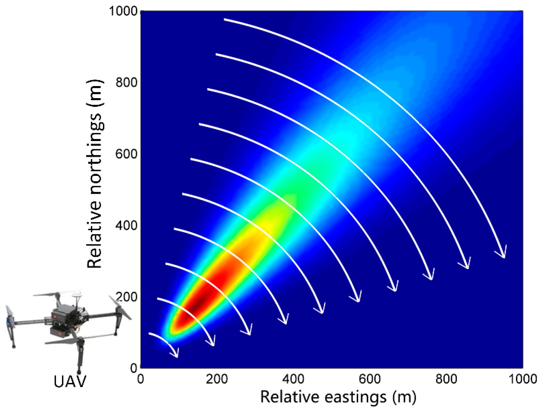
Ideally, the observations of air contaminant dispersion should be collected in the real situation by UAVs. However, due to the lack of field experiment conditions, the observations in our experiments are assumed to be collected by the 10 virtual UAVs with their trajectories at the height of 30 m AGL. To effectively acquire observations, the trajectories of UAVs are designed according to the wind direction. According to the setting of sensors in the Indianapolis experiment [16], the trajectories of UAVs are designed as arcs through the plume. For example, when the wind direction is 220°, trajectories are shown in Figure 2. There are 10 simulated arc trajectories through the plume, each of which corresponds to a UAV (but only one UAV is shown in the figure). Each UAV is assumed to move back and forth along its own trajectory and collect the concentration data at the trajectory point (not the average concentration) sequentially until the end of the experiment. The duration of data collection is therefore the same as the duration of the experiment (100 min). The flight speed of all virtual UAVs is assumed to be 2 m/s, and therefore, the flight time for a lap (forth and back) of the longest trajectory (about 1900 m) is about 16 min. In addition, all UAVs are assumed to collect data simultaneously. The time interval of UAV data collection is set according to the characteristics of gas sensors in the UAV system. In our experiments, it is set as 1 min.
3.2. Parameter Configuration
This section illustrates the parameter configuration of the two experiments and “real” dispersions. These parameters include the release rate and four dispersion coefficients. The release rate, which significantly influences the size and shape of the plume, is difficult to measure accurately. In Experiment 1, the known release rate is not the parameter to be estimated. Therefore, the release rates in the “real” dispersion and two groups of Experiment 1 are all set to be constant at 30 g/s. In the contaminant gas leakage incidents, the release rate is one of the state parameters to be estimated. Thus, in the “real” dispersion, it is considered to be variable to test the data assimilation method. An exponential decay curve is applied to describe the variation of the release rate because in some cases the release rate decreases with the reduction of the amount of residual contaminant [18].
As for the four dispersion coefficients, the “real” dispersions use variant dispersion coefficients to simulate the “true” situation. The four dispersion coefficients are closely correlated with the environmental conditions, such as the atmospheric stability and terrain. The Pasquill-Gifford-Turner (henceforth P-G-T) [17,19,20] approach is widely used in the classification of atmospheric stability. Based on the approach, the P-G-T curves are developed to identify the four dispersion coefficients according to the atmospheric stability class. Unfortunately, this approach takes few terrain conditions into consideration. Furthermore, there are many other researchers having provided empirical values of the four coefficients under different atmospheric stability classes and terrain conditions, such as Briggs [21] and Vogt [22]. Carrascal [23] compared these empirical values under identical atmospheric conditions. In the “real” dispersions of two experiments, the parameter scheme of Vogt is adopted to describe the variation of four dispersion coefficients in chemical industry parks. The values of four coefficients according to Vogt are shown in Table 2. This table gives empirical values of a, b, c, and d under different atmospheric stability classes for open country. In this table, Class A to F represents different atmospheric stability classes. Class A represents the most active class, and Class F is the most stable one. As for the terrain condition, with few obstacles like huge buildings, the open country is similar to the terrain of chemical industry parks. Therefore, the parameter scheme of Vogt is suitable for the identification of the four dispersion coefficients in chemical industry parks. In the “real” dispersion of Experiment 1, the atmospheric stability is considered to vary following the order of A, B, C, and D during 120 min (only the duration of 0 to 100 min is simulated). Thus, the values of state parameters (a, b, c, and d) under class A, B, C, and D are selected as their values at 0, 40, 80, 120 min in the “real” dispersion, respectively. In addition, the four dispersion coefficients between two classes of atmospheric stability are assumed to change gradually and linearly. In the “real” dispersion of Experiment 2, the four dispersion coefficients follow a similar variation rule (change gradually and linearly), except that the variation is slowed down to lower the difficulty of the data assimilation. Some key values of coefficients in the “real” dispersions of the two experiments are shown in Table 3. In contrast, the four dispersion coefficients in Experiment 1A are initialed to the values under Class A and considered to stay constant before the updates to the “true” values of the “real” dispersion every 40 min (blue dash lines in Figure 3). The update is designed to enhance the prediction accuracy of the conventional dispersion model. Therefore, the experimental atmospheric stability in Experiment 1A (using the Gaussian dispersion model without data assimilation) shows step changes because we assume that these parameters are observed and updated each 40 min. Additionally, in the data assimilation models of Experiment 1B and Experiment 2, the particles representing four dispersion coefficients are initialized with ranges covering the variation range mentioned above.
These numerical experiments are implemented as follows. Before the two experiments, the “real” dispersions with the variant parameters are firstly executed to generate the “true” concentrations. After that, the observations are produced from the “true” concentrations by the simulated trajectories of UAVs and the measurement model. Then, in the two experiments, the observations are assimilated into the Gaussian plume model by the proposed data assimilation methods to generate the concentration distribution. Additionally, in Experiment 1, Experiment 1A is implemented as the control group to generate the concentration prediction without data assimilation.
4. Results
4.1. Experiment 1
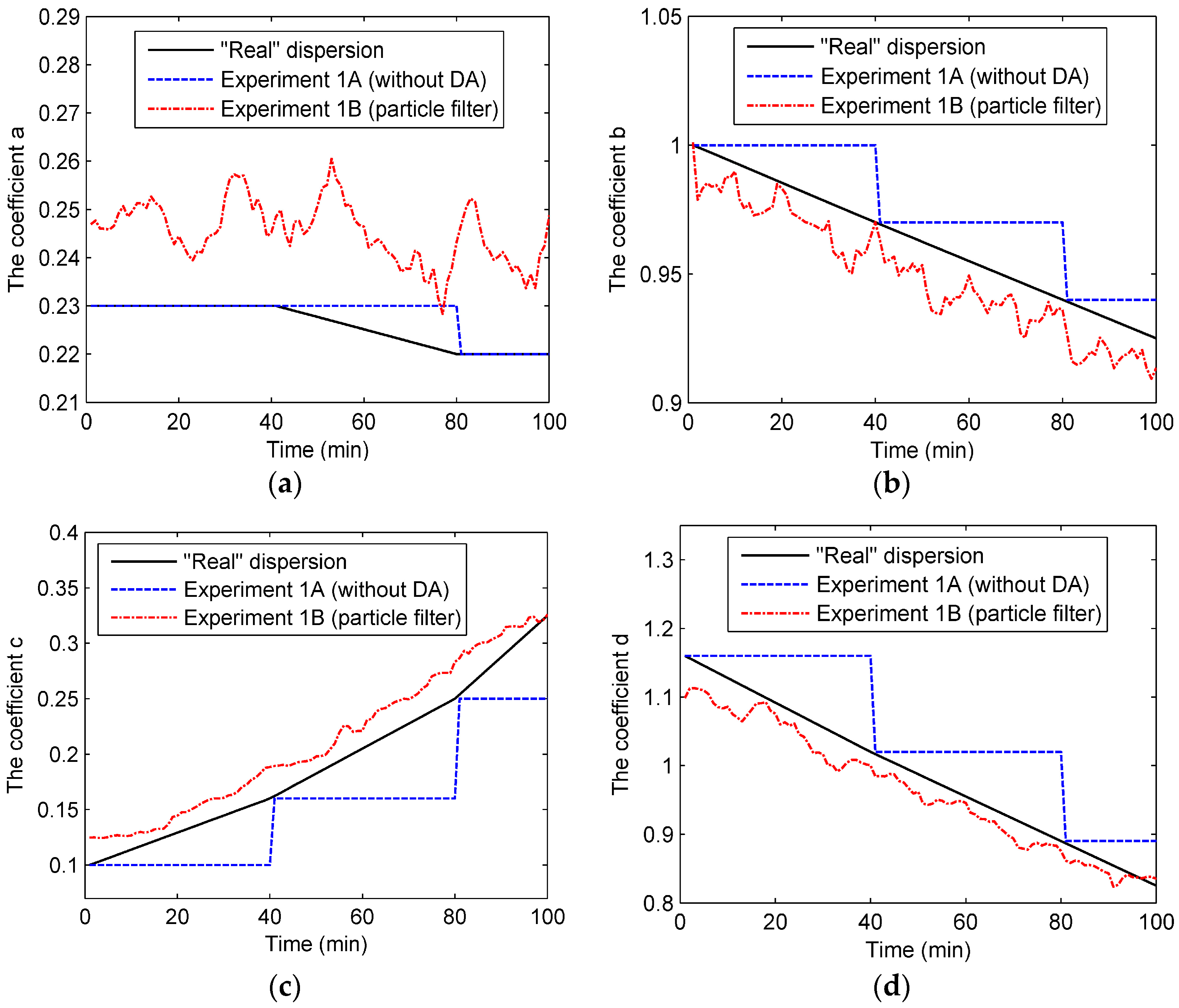
Figure 3 shows the state parameters (a, b, c, and d) in Experiment 1. As can be seen from the figure, the dispersion coefficients in the “real” dispersion follow the piecewise-linear variation according to Table 3. As for the dispersion coefficients in Experiment 1B, they are close to the “true” values of the “real” dispersion. With the particle filter, these coefficients follow the trend of the “true” values closely. In comparison, without data assimilation, the coefficients in Experiment 1A stay invariant before the updates to the “true” values. However, it is worth mentioning that the particle filter’s performance in estimating coefficient a is less effective than the performances for others. Indeed, coefficient a in Experiment 1A is even closer to the “true” value than that of Experiment 1B. This might be because of the flat variation of coefficient a.
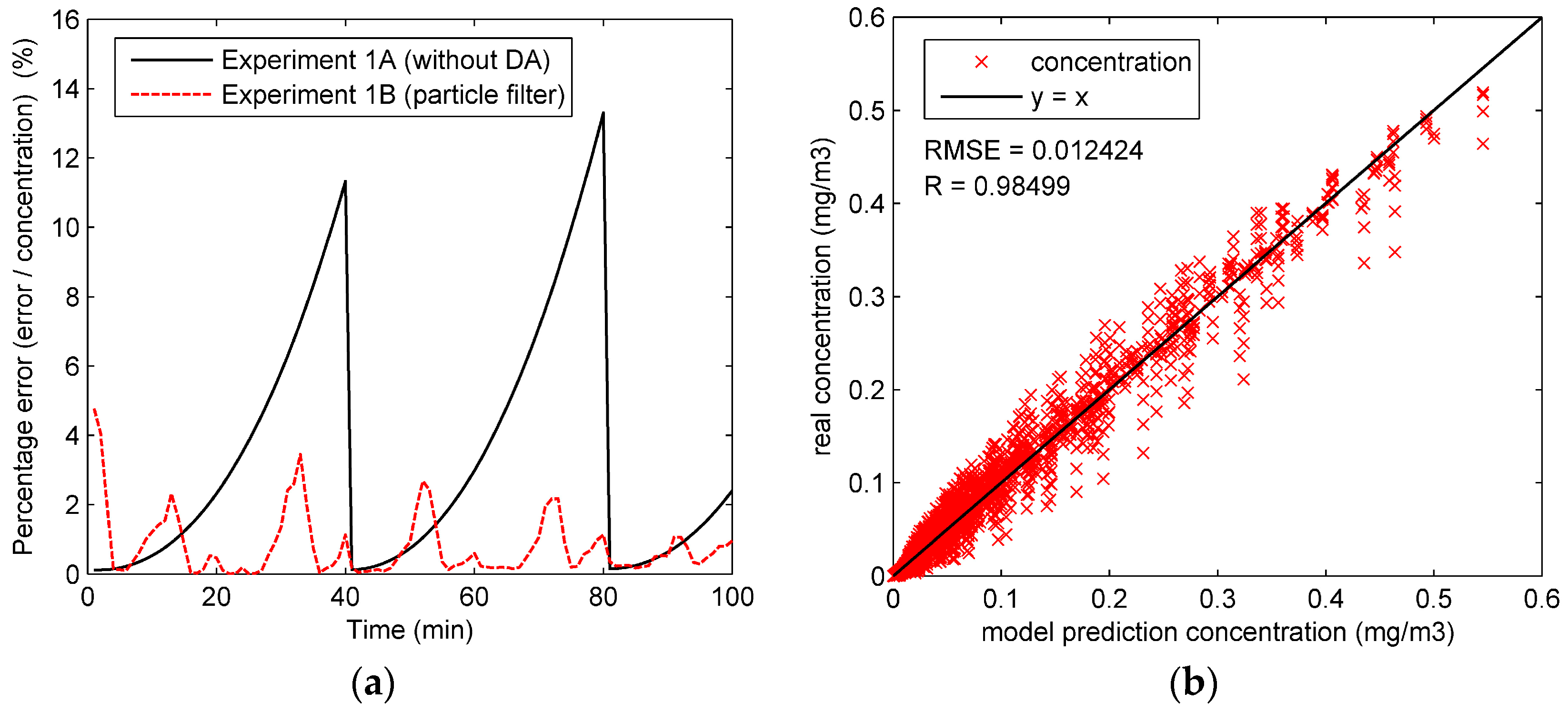
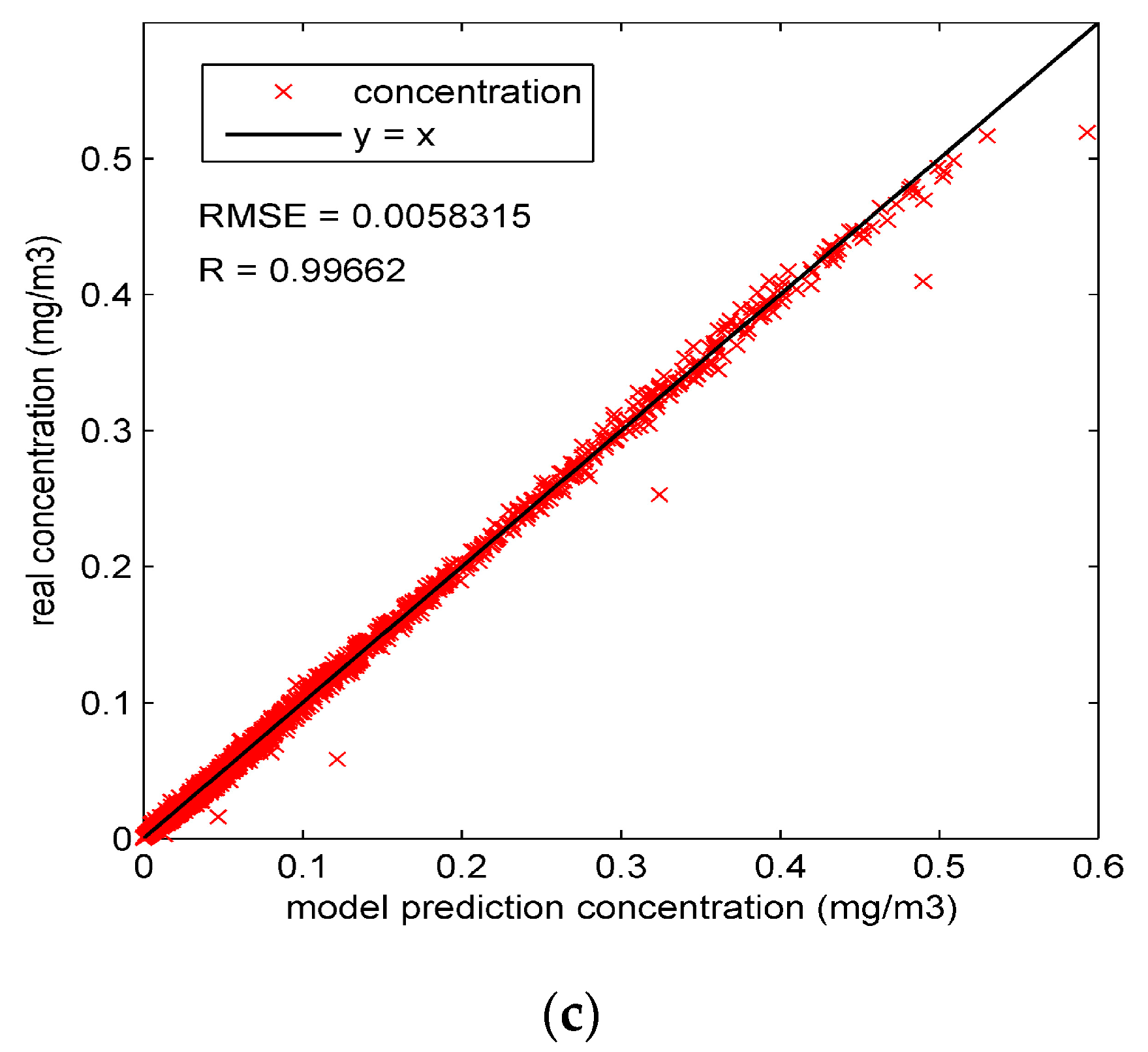
To observe the performance of particle filter on the concentration prediction in Experiment 1, the percentage error of the whole region is calculated by dividing the average error by the concentration, as shown in Figure 4a. It can be seen from this figure that the percentage error of Experiment 1B is significantly lower than that of Experiment 1A in most of the experiment duration. The ascendant percentage error curve of Experiment 1A in Figure 4a comes from the errors of four dispersion coefficients. As shown in Figure 3, without data assimilation, four dispersion coefficients stay constant before the updates in Experiment 1A. Therefore, the errors of the four coefficients grow over time, consequently causing the ascendant percentage error curve in Figure 4a. In comparison, with the state parameters calibrated by particle filter, the percentage error of Experiment 1B is reduced to a relatively low level. In most of the experiment duration, the percentage error with particle filter is lower than 4%. Figure 4b,c compare the “true” concentrations and the model prediction concentrations in Experiment 1 and show the root mean square error (RMSE) and correlation coefficient (R). In comparison, most of the concentrations in the Figure 4c are more concentrated around the line “y = x” than those of Figure 4b, illustrating that the model predictions with particle filter are closer to the “true” concentrations. Further, the higher correlation coefficient (0.99662) and lower RMSE (0.0058315) of Experiment 1B also illustrate the good performance of particle filter.
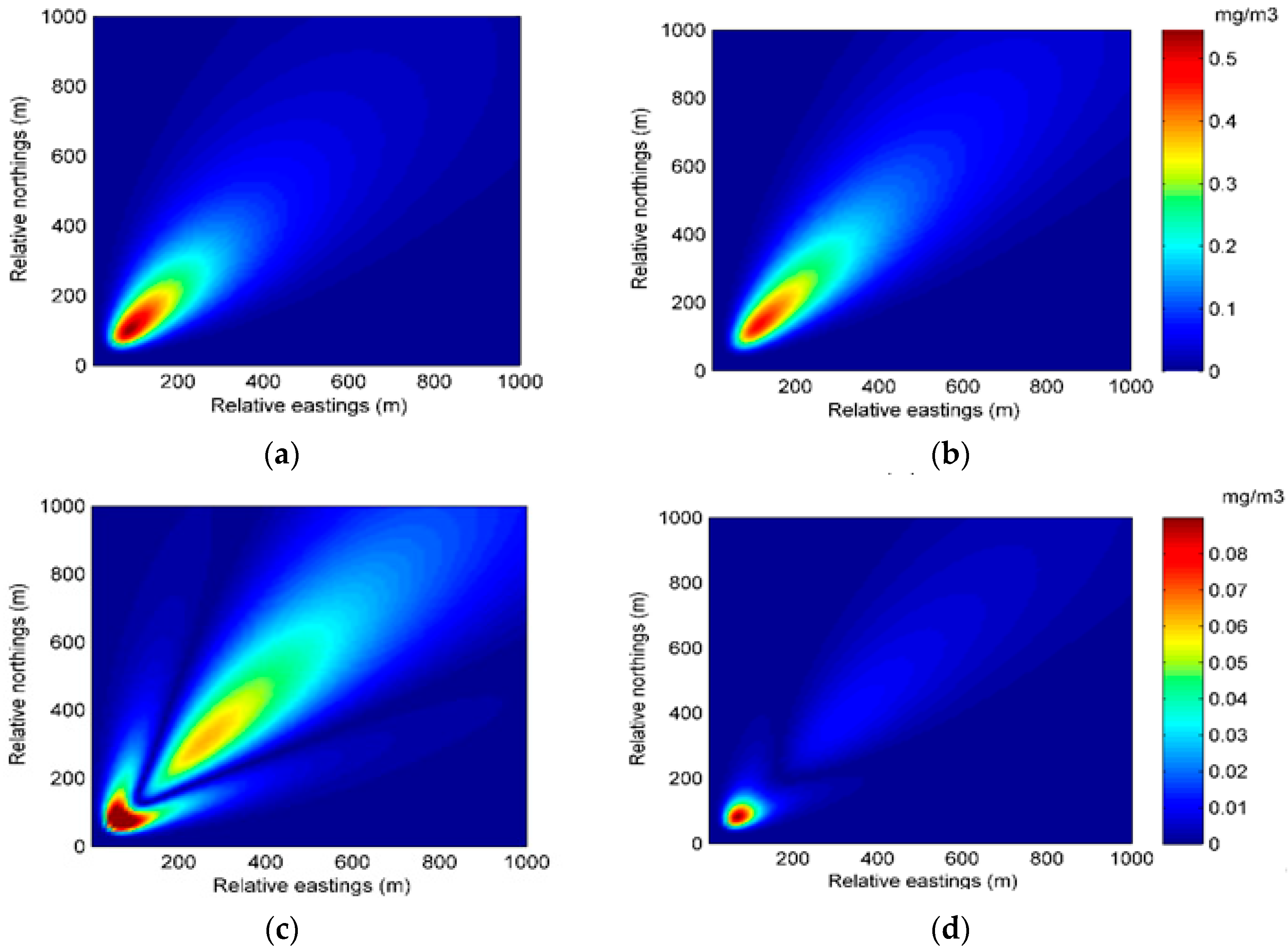
A similar conclusion can be drawn from the spatial distribution of the predicted concentration and error in Experiment 1. Figure 5 and Figure 6 show the spatial distributions of predicted concentration and error at 35 min and 70 min, respectively. As can be seen from the figures, with data assimilation, the result of Experiment 1B has a more accurate prediction distribution of concentration and lower error in most of the region.
4.2. Experiment 2
Experiment 2 compares the performances of particle filter and the particle filter combining the EM algorithm. Figure 7 shows the state parameters (a, b, c, d and release rate) in Experiment 2.
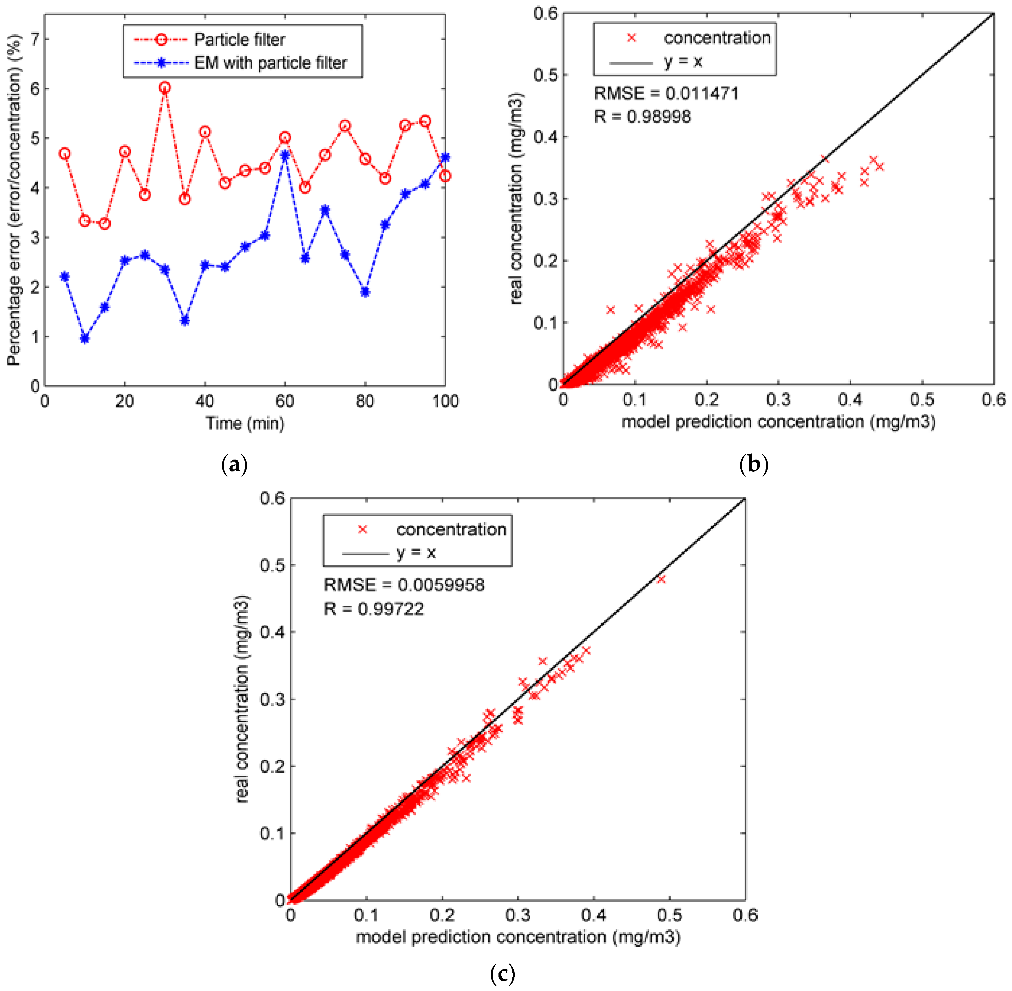
As can be seen from the figure, the performance of particle filter is unsatisfactory, and the estimations of coefficients are far from the “true” values, especially for coefficient c, which may result from the high dimension of state parameters. With the high dimension of state parameters, it is difficult for particle filter to estimate , , , and simultaneously. In contrast, the estimation accuracy of the EM algorithm with particle filter is slightly better than particle filter because the EM algorithm decreases the complexity of parameter estimation by dividing the parameter estimation process into two steps. As for the percentage error of the whole region, it is calculated and shown in Figure 8a. In addition, the RMSE and R values of all predicted concentrations in Experiment 2 are shown in Figure 8b,c. The similar conclusion can be drawn from Figure 8, which shows that the performance of the EM algorithm with particle filter is slightly better than typical particle filter since the result of Experiment 2B shows a smaller RMSE value and higher R value.
The better performance of the EM algorithm with particle filter can also be seen from the spatial distributions of predicted concentration and error. Figure 9 and Figure 10 show the spatial distributions of predicted concentration and error at 35 min and 70 min in Experiment 2, respectively. It can be seen from the two figures that the distribution of the predicted concentration of Experiment 2B is more accurate, illustrating the better performance of the EM algorithm with particle filter.
From the results, we can conclude that adding the EM step indeed improves the performance of the data assimilation. However, meanwhile, it introduces larger computational complexity. Table 4 displays the prediction accuracy and total running time of the two proposed data assimilation methods in Experiment 2. It can be seen from this table that compared to the particle filter, although adding the EM step reduces the RMSE by about 50%, it also brings more than 10 times the total running time. In general, the prediction accuracy of the two methods is acceptable in most cases. Therefore, the particle filter is a better alternative when there is a strict requirement of real time while the EM algorithm with particle filter is superior if the prediction accuracy is preferred.
4.3. Noise Analysis
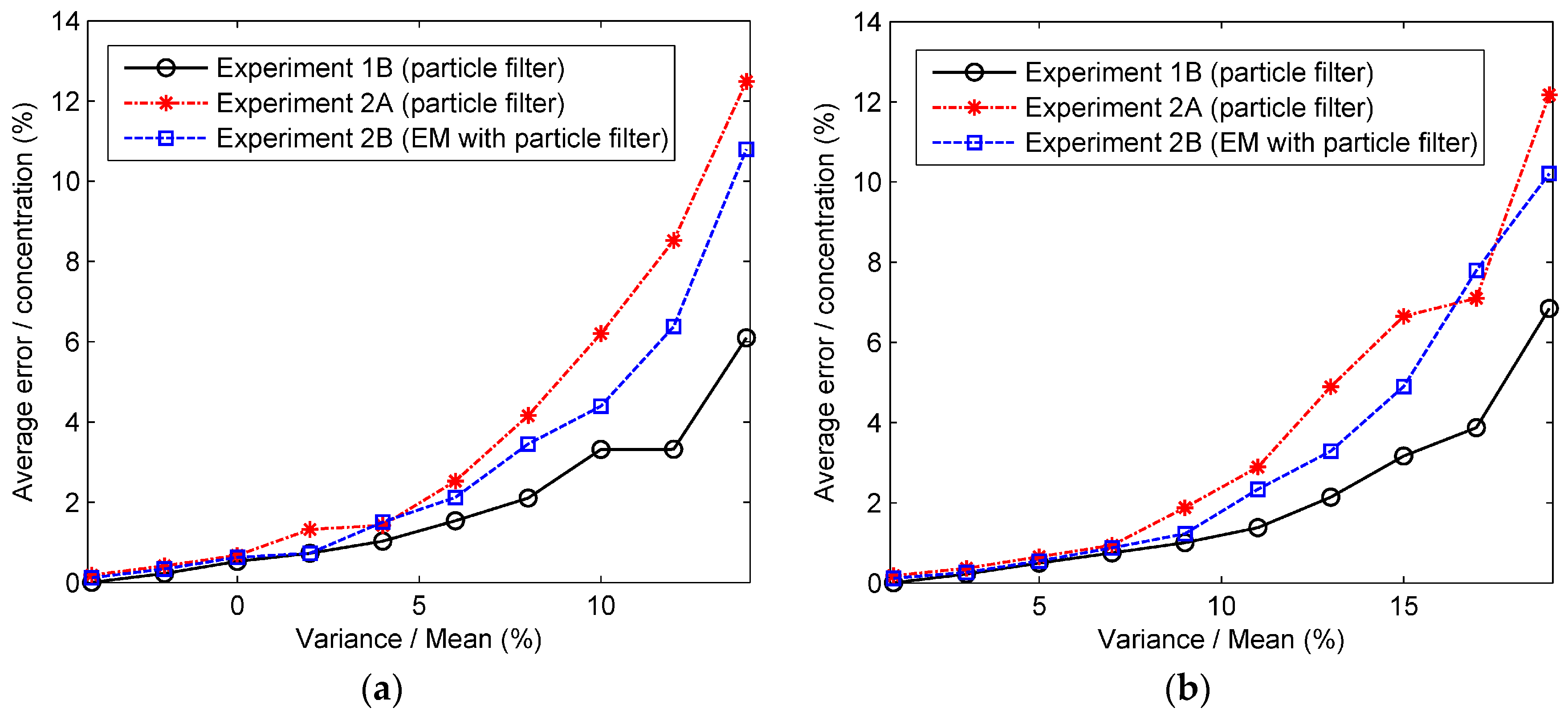
The results of two experiments show the good performances of the data assimilation methods proposed. However, the results of our experiments are ideal because the observed data are generated from the Gaussian model instead of the real environment. Therefore, there are differences between the very ideal world analyzed in this paper and the real world. The measurement noise is an important factor influencing the differences. We have therefore analyzed the performances of the proposed data assimilation methods with different amplitudes of measurement error. The measurement noise is assumed to be Gaussian white noise following the Gaussian distribution . The percentage error with different relative variance is calculated and shown in Figure 11. The relative variance is expressed as the variance of measurement error divided by the measurement mean (“true” concentration). It can be seen from the figure that with the relative variance increasing, the percentage errors of all predicted concentrations grow drastically. The results illustrate that the performance of the data assimilation method depends on the measurement noise. Moreover, for a more detailed observation of the performances of data assimilation methods, the percentage errors with different amplitudes of relative variance at 35 min and 70 min are displayed in Figure 12. Similar trends can be seen from the figure that the percentage errors grow rapidly with the relative variance increasing. In addition, we can also conclude from these figures that the EM algorithm with particle filter performs better in terms of prediction accuracy than typical particle filter in Experiment 2.
5. Discussion
In the two numerical experiments, the performances of particle filter and the method of particle filter combining the EM algorithm are tested. The results illustrate that the dimension of state parameters significantly affects the quality of data assimilation. In Experiment 1, where the state parameters are only four dispersion coefficients, the data assimilation based on the particle filter is effective for estimating the state parameters and improving the model prediction. However, when the dimension of state parameters becomes higher in Experiment 2, the estimation accuracy of typical particle filter decreases because the particles with a high dimension are hard to converge to a satisfactory result. In contrast, the method of particle filter combining the EM algorithm performs slightly better in terms of the estimation accuracy in Experiment 2. By iteratively computing the five state parameters in the E-step and M-step, respectively, the EM algorithm with particle filter reduces the complexity of the estimation and improves the estimation results. Another factor influencing the results is the number of particles. On the one hand, each particle represents the system state in our work. Thus, the larger number of particles means more diverse dispersion states, which is beneficial to the estimation of system state. On the other hand, the large number of particles will increase the computational cost because the transition and measurement model are calculated for each particle. In our work, 150, 250, and 150 particles are used in the particle filter of Experiment 1B, 2A, and 2B, respectively. The high accuracy of results and acceptable efficiency prove that these particle numbers are feasible in our experiments.
In terms of the drawbacks of these experiments, one is the wind field, which significantly influences the dispersion, is considered to be stable and uniform in our work. However, the actual wind field is relatively dynamic and complex. Therefore, the dynamic modeling of the wind field should be a research focus in future works. Another drawback is from the EM algorithm. The method of particle filter combining the EM algorithm performs better in the second case, but the EM algorithm is likely to converge to a local optimum, which may lead to the missing of the global optimum. In addition, as for the observations, in this paper they are assumed to be collected by the virtual UAV along the trajectory. However, when the UAV is used to collect data in the field experiment, there are a number of problems, such as the atmospheric flow change caused by the propellers of helicopter-style UAV and the selection of the sensors’ location [24]. Therefore, these problems caused by UAV will be discussed in the implementation of the field experiment in future works. In addition, the Non-helicopter-style UAVs could be a better alternative data collection platform for future uses. Moreover, the Gaussian plume model is a steady model and not strictly applicable to the variant atmospheric stability and emission rate in this paper. There is a time lag between the change in the emission rate or atmospheric stability and the change in concentration distribution. For simplicity, this time lag is not considered in this paper because the model considering the time lag like the Gaussian multi-puff model will generate a large computational cost and fail to meet the requirement of real-time. If the time lag is considered, the problem of the large computational cost will be focused on in future works.
Due to the ideal model and conditions, this paper is a starting point for data assimilation research in air contaminant dispersion. The ideal model and virtual observations in this paper are acceptable at the current stage because the focus of this paper is to preliminarily test the proposed data assimilation methods. The results illustrate the satisfactory performance of the proposed data assimilation methods for state parameter estimations and the prediction accuracy, although the model and conditions are different from the real environment. Further, later work will utilize a more accurate dispersion model and gradually place the test case in more realistic conditions. In addition, the data collected by a number of real UAV sensory systems in the chemical industry cluster will be used as observations in the final application, as expected in this paper.
6. Conclusions
In this paper, two data assimilation methods using particle filter and the method of particle filter combining the EM algorithm are developed to improve the accuracy of air contaminant dispersion predictions based on the Gaussian plume model. The architecture of the data assimilation model is presented. Then, numerical experiments corresponding to two emission cases are designed and implemented to test the performances of the proposed data assimilation methods. It should be noted that the measurement error is considered in the numerical experiments to generate more realistic observations. The results show that the particle filter can effectively improve the accuracy of model predictions when the dimension of state parameters is relatively low. In contrast, when the dimension of state parameters becomes higher (the second case), the method of particle filter combining the EM algorithm performs better than the typical particle filter in the estimation accuracy. Therefore, these proposed data assimilation methods provide strong support for the prediction of air contaminant dispersion and emergency management in chemical industry parks. Future works should include implementing the field experiment in chemical industry parks to verify the data assimilation methods in real situations and dynamic modeling of the wind field for a more accurate prediction of the atmospheric dispersion model.
Acknowledgments
This study is supported by National Key Research and Development (R&D) Plan under Grant No. 2017YFC0803300 and the National Natural Science Foundation of China under Grant Nos. 71673292,61503402 and Guangdong Key Laboratory for Big Data Analysis and Simulation of Public Opinion.
Author Contributions
Rongxiao Wang and Sihang Qiu conceived and designed the experiments; Rongxiao Wang performed the experiments under the guidance of Bin Chen; Zhengqiu Zhu analyzed the data; Xiaogang Qiu gave important suggestions for data analysis; Rongxiao Wang wrote the paper.
Conflicts of Interest
The authors declare no conflict of interest.
References
- Bouttier, F.; Courtier, P. Data assimilation Concepts and Methods; Meteorological Training Course Lecture Series; ECMWF: Reading, UK, 1999. [Google Scholar]
- Xue, H.; Gu, F.; Hu, X. Data assimilation using sequential monte carlo methods in wildfire spread simulation. ACM TOMACS 2012, 22, 1–25. [Google Scholar] [CrossRef]
- Yan, X.; Gu, F.; Hu, X.; Guo, S. A dynamic data driven application system for wildfire spread simulation. In Proceedings of the Winter Simulation Conference, Austin, TX, USA, 13–16 April 2009; pp. 3121–3128. [Google Scholar]
- Krysta, M.; Bocquet, M.; Sportisse, B.; Isnard, O. Data assimilation for short-range dispersion of radionuclides: An application to wind tunnel data. Atmos. Environ. 2006, 40, 7267–7279. [Google Scholar] [CrossRef]
- Kalman, R.E. A new approach to linear filtering and prediction problems. J. Basic Eng. 1960, 82, 35–45. [Google Scholar] [CrossRef]
- Pastres, R.; Ciavatta, S.; Solidoro, C. The Extended Kalman Filter (EKF) as a tool for the assimilation of high frequency water quality data. Ecol. Model. 2003, 170, 227–235. [Google Scholar] [CrossRef]
- Evensen, G. The ensemble kalman filter: Theoretical formulation and practical implementation. Ocean Dyn. 2003, 53, 343–367. [Google Scholar] [CrossRef]
- Reddy, K.V.U.; Yang, C.; Tarunraj, S.; Scott, P.D. Data assimilation in variable dimension dispersion models using particle filters. In Proceedings of the 10th International Conference on Information Fusion, Quebec, QC, Canada, 9–12 July 2007. [Google Scholar]
- Gordon, N.J.; Salmond, D.J.; Smith, A.F.M. Novel approach to nonlinear/non-gaussian bayesian state estimation. IEE Proc. F Radar Signal Process. 1993, 140, 107–113. [Google Scholar] [CrossRef]
- Ng, S.K.; Krishnan, T.; McLachlan, G.J. The em algorithm. In Handbook of Computational Statistics: Concepts and Methods; Gentle, J.E., Härdle, W.K., Mori, Y., Eds.; Springer: Berlin/Heidelberg, Germany, 2012; pp. 139–172. [Google Scholar]
- Zhao, Z.; Huang, B.; Liu, F. Parameter estimation in batch process using em algorithm with particle filter. Comput. Chem. Eng. 2013, 57, 159–172. [Google Scholar] [CrossRef]
- Kim, H.-D.; Komatani, K.; Ogata, T.; Okuno, H.G. Real-time auditory and visual talker tracking through integrating em algorithm and particle filter. In New Trends in Applied Artificial Intelligence, Proceedings of the 20th International Conference on Industrial, Engineering and Other Applications of Applied Intelligent Systems, IEA/AIE 2007, Kyoto, Japan, 26–29 June 2007; Okuno, H.G., Ali, M., Eds.; Springer: Berlin, Heidelberg, 2007; pp. 280–290. [Google Scholar]
- Yang, H.; Huang, Y.; Center, S.E. Evaluating atmospheric pollution of chemical plant based on Unmanned Aircraft Vehicle(UAV). J. Geo-Inf. Sci. 2015, 17, 1269–1274. [Google Scholar]
- Hirst, B.; Jonathan, P.; González del Cueto, F.; Randell, D.; Kosut, O. Locating and quantifying gas emission sources using remotely obtained concentration data. Atmos. Environ. 2013, 74, 141–158. [Google Scholar] [CrossRef]
- White, B.; Tsourdos, A.; Ashokaraj, I.; Subchan, S.; Zbikowski, R. Contaminant cloud boundary monitoring using uav sensor swarms. In Proceedings of the AIAA Guidance, Navigation and Control Conference, Boston, MA, USA, 20–23 August 2007. [Google Scholar]
- Scire, J.S.G.; Strimaitis, D.; Yamartino, R. A User’s Guide for the Calpuff Dispersion Model; Earth Tech., Inc.: Concord, MA, USA, 2000. [Google Scholar]
- Pasquill, F. The estimation of the dispersion of windborne material. Aust. Meteorol. Mag. 1961, 90, 33–49. [Google Scholar]
- Qiu, S.; Chen, B.; Zhu, Z.; Wang, Y.; Qiu, X. Source term estimation using air concentration measurements during nuclear accident. J. Radioanal. Nucl. Chem. 2017, 311, 165–178. [Google Scholar] [CrossRef]
- Turner, D.B. A diffusion model for an urban area. J. Appl. Meteorol. 1964, 3, 83–91. [Google Scholar] [CrossRef]
- Gifford, F.A., Jr. Use of routine meteorological observations for estimating atmospheric dispersion. Nucl. Saf. 1961, 2, 47–51. [Google Scholar]
- Briggs, G.A. Diffusion Estimation for Small Emissions; Atmospheric Turbulence and Diffusion Laboratory; NOAA: Silver Spring, MD, USA, 1973; Volume 79, p. 83.
- Vogt, K.J. Empirical investigations of the diffusion of waste air plumes in the atmosphere. Nucl. Technol. 1977, 34, 43–57. [Google Scholar] [CrossRef]
- Carrascal, M.D.; Puigcerver, M.; Puig, P. Sensitivity of gaussian plume model to dispersion specifications. Theor. Appl. Climatol. 1993, 48, 147–157. [Google Scholar] [CrossRef]
- Villa, T.F.; Salimi, F.; Morton, K.; Morawska, L.; Gonzalez, F. Development and validation of a UAV based system for air pollution measurements. Sensors 2016, 16, 2202. [Google Scholar] [CrossRef] [PubMed]
Figure 1.
Data assimilation based on the particle filter.
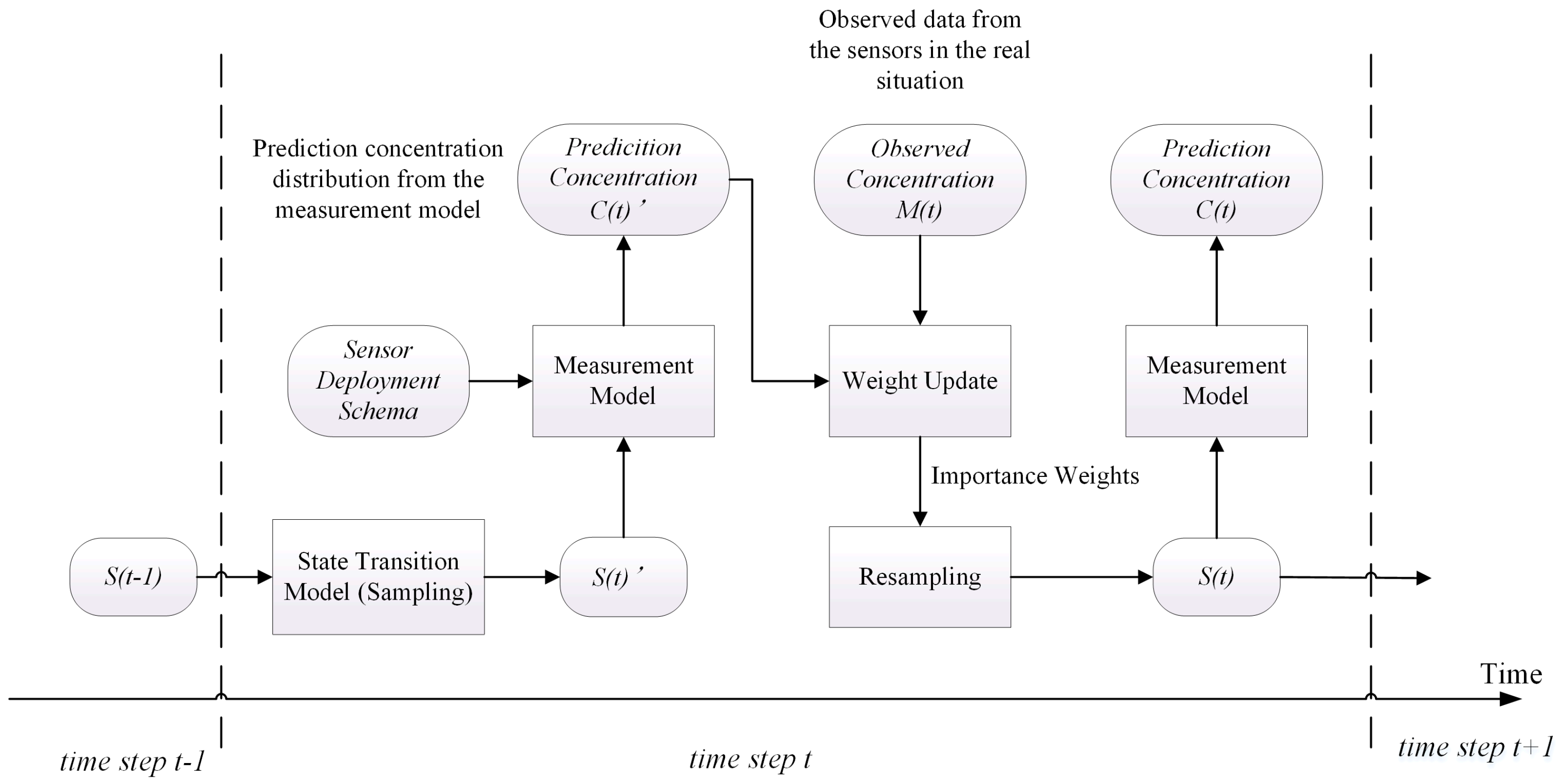
Figure 2.
Trajectories of UAVs when the wind direction is 220°.

Figure 3.
Four coefficients of dispersion in Experiment 1: (a) coefficient a; (b) coefficient b; (c) coefficient c; (d) coefficient d.
Figure 3.
Four coefficients of dispersion in Experiment 1: (a) coefficient a; (b) coefficient b; (c) coefficient c; (d) coefficient d.

Figure 4.
The assimilation results of the whole region in Experiment 1: (a) percentage error of the whole region in Experiment 1A and 1B; (b) the “true” concentrations and model prediction concentrations in Experiment 1A; (c) the “true” concentrations and model prediction concentrations in Experiment 1B.


Figure 5.
The spatial distributions of the predicted concentration and error at 35 min in Experiment 1: (a) spatial distribution of the predicted concentration of Experiment 1A; (b) spatial distribution of the predicted concentration of Experiment 1B; (c) spatial distribution of the error of Experiment 1A; (d) spatial distribution of the error of Experiment 1B.

Figure 6.
The spatial distributions of the predicted concentration and error at 70 min in Experiment 1: (a) spatial distribution of the predicted concentration of Experiment 1A; (b) spatial distribution of the predicted concentration of Experiment 1B; (c) spatial distribution of the error of Experiment 1A; (d) spatial distribution of the error of Experiment 1B.
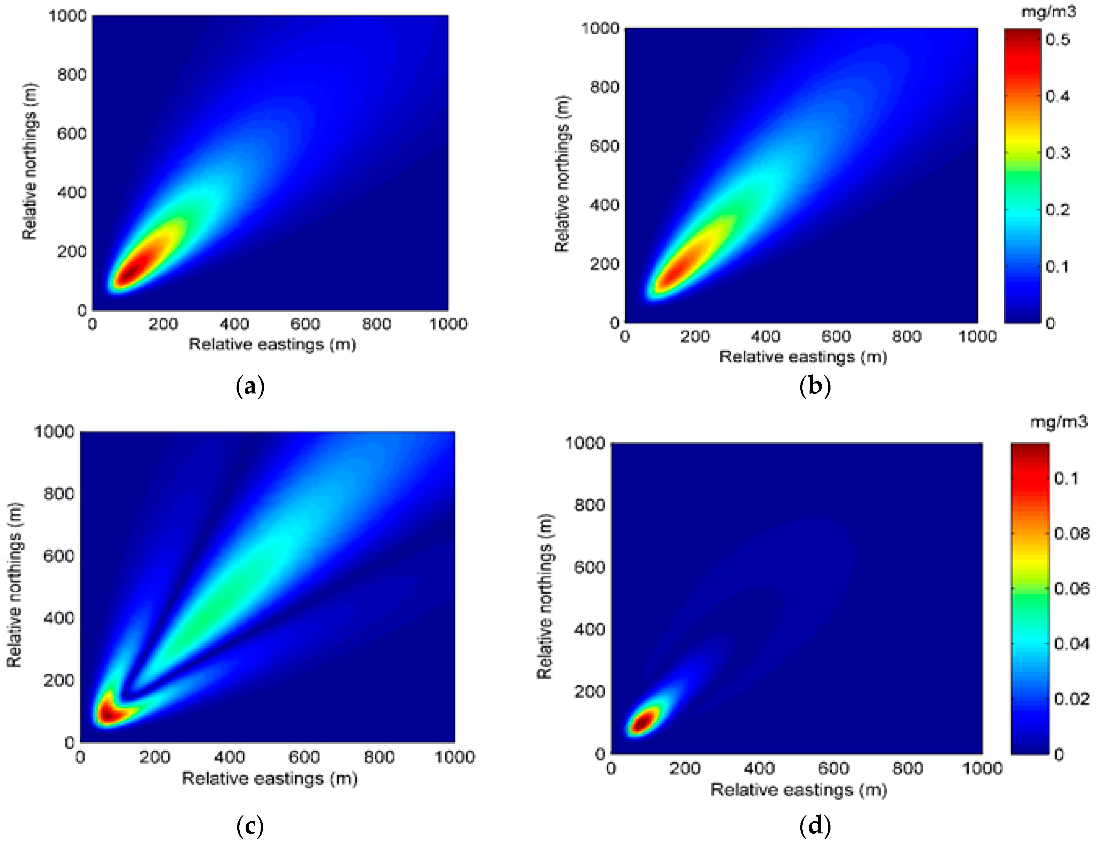
Figure 7.
Four dispersion coefficients and the release rate in Experiment 2: (a) coefficient a; (b) coefficient b; (c) coefficient c; (d) coefficient d; (e) release rate.
Figure 7.
Four dispersion coefficients and the release rate in Experiment 2: (a) coefficient a; (b) coefficient b; (c) coefficient c; (d) coefficient d; (e) release rate.
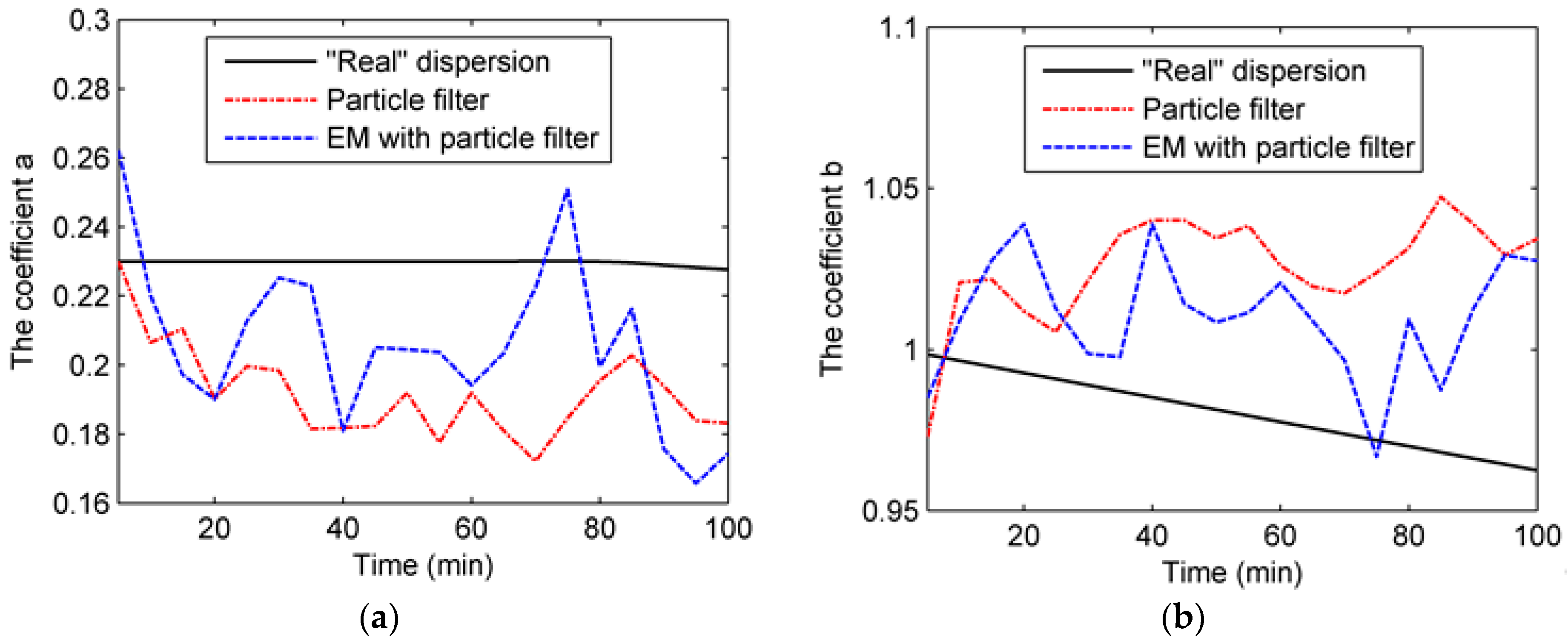
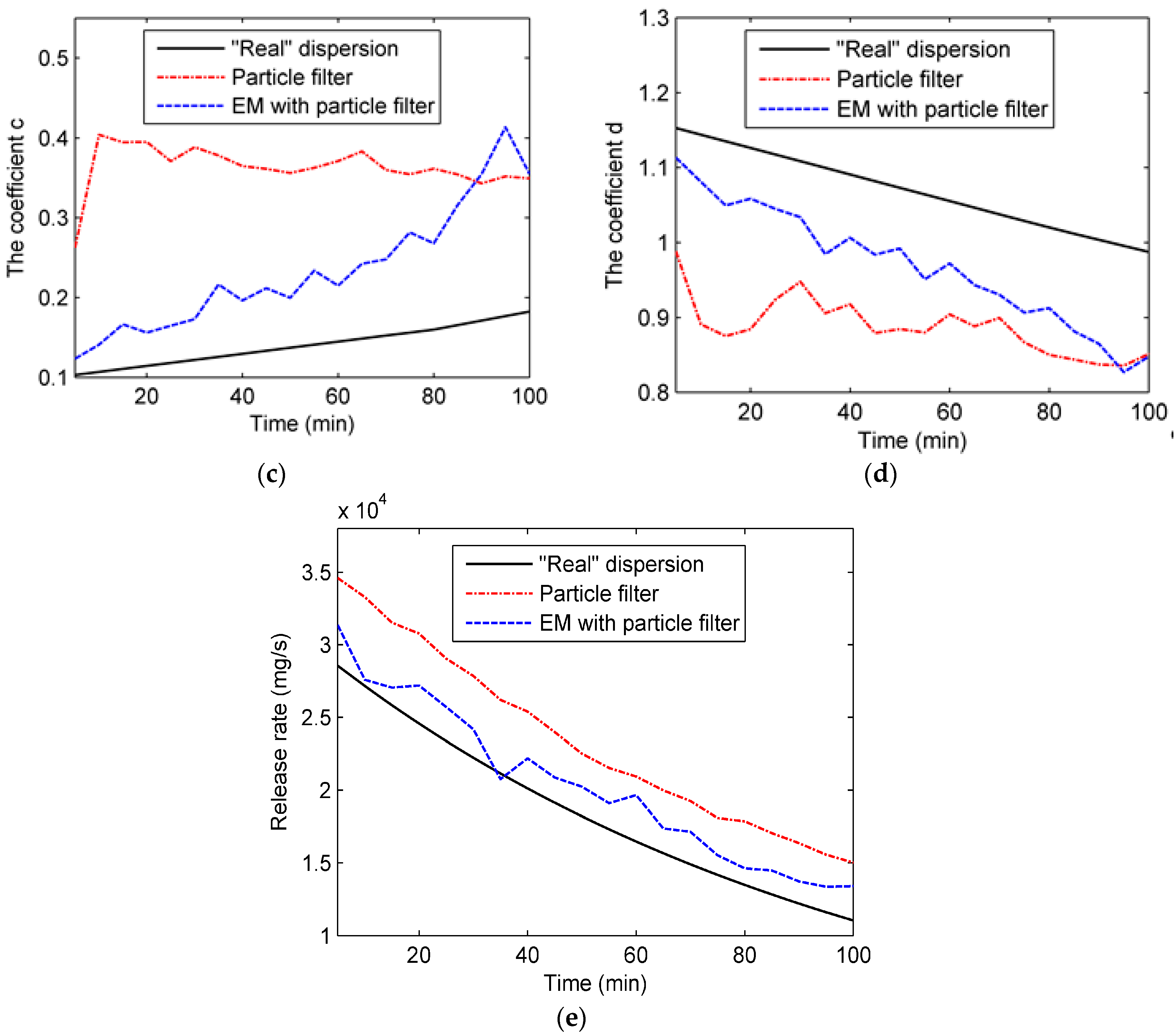
Figure 8.
The assimilation results of the whole region in Experiment 2: (a) percentage error of the whole region in Experiment 2A and 2B; (b) the “true” concentrations and model prediction concentrations in Experiment 2A; (c) the “true” concentrations and model prediction concentrations in Experiment 2B.

Figure 9.
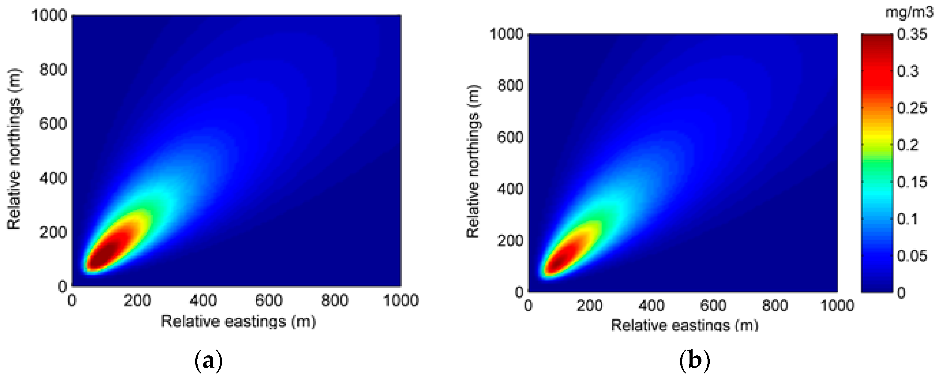
The spatial distributions of the predicted concentration and error at 35 min in Experiment 2: (a) spatial distribution of the predicted concentration of Experiment 2A; (b) spatial distribution of the predicted concentration of Experiment 2B; (c) spatial distribution of the error of Experiment 2A; (d) spatial distribution of the error of Experiment 2B.
Figure 9.
The spatial distributions of the predicted concentration and error at 35 min in Experiment 2: (a) spatial distribution of the predicted concentration of Experiment 2A; (b) spatial distribution of the predicted concentration of Experiment 2B; (c) spatial distribution of the error of Experiment 2A; (d) spatial distribution of the error of Experiment 2B.


Figure 10.
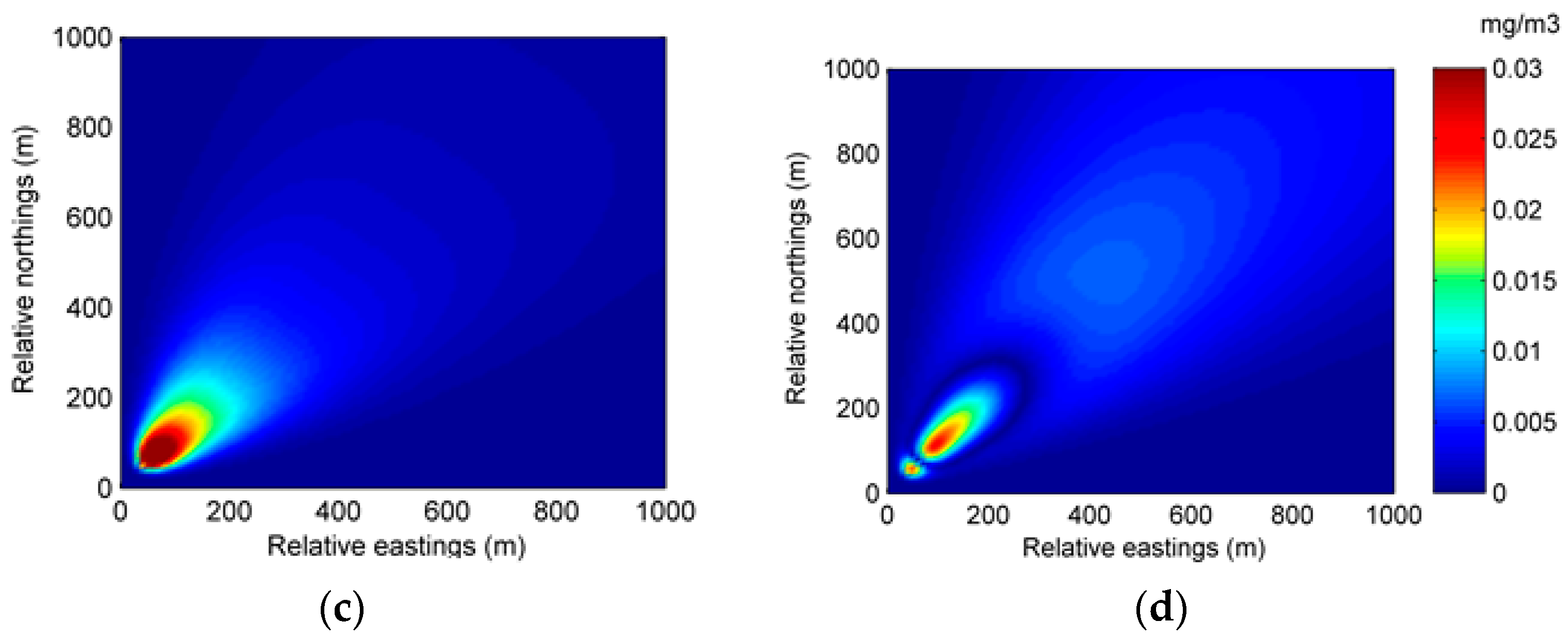
The spatial distributions of the predicted concentration and error at 70 min in Experiment 2: (a) spatial distribution of the predicted concentration of Experiment 2A; (b) spatial distribution of the predicted concentration of Experiment 2B; (c) spatial distribution of the error of Experiment 2A; (d) spatial distribution of the error of Experiment 2B.
Figure 10.
The spatial distributions of the predicted concentration and error at 70 min in Experiment 2: (a) spatial distribution of the predicted concentration of Experiment 2A; (b) spatial distribution of the predicted concentration of Experiment 2B; (c) spatial distribution of the error of Experiment 2A; (d) spatial distribution of the error of Experiment 2B.
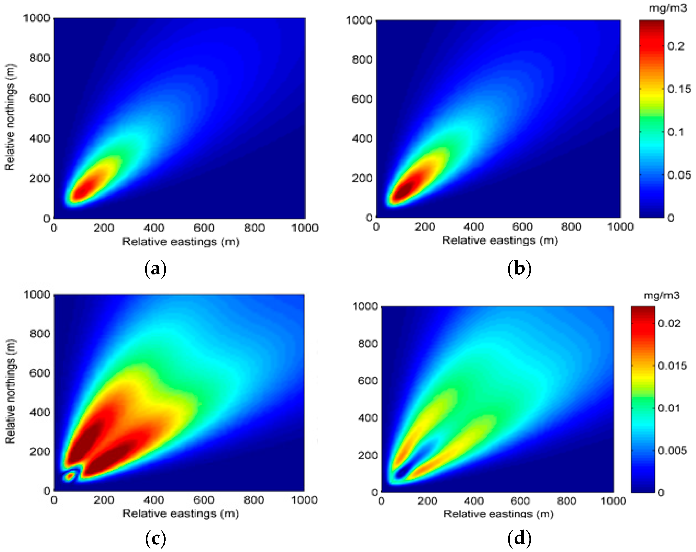
Figure 11.
Percentage errors of all predicted concentrations in the numerical experiments with different relative variance of measurement noise.
Figure 11.
Percentage errors of all predicted concentrations in the numerical experiments with different relative variance of measurement noise.
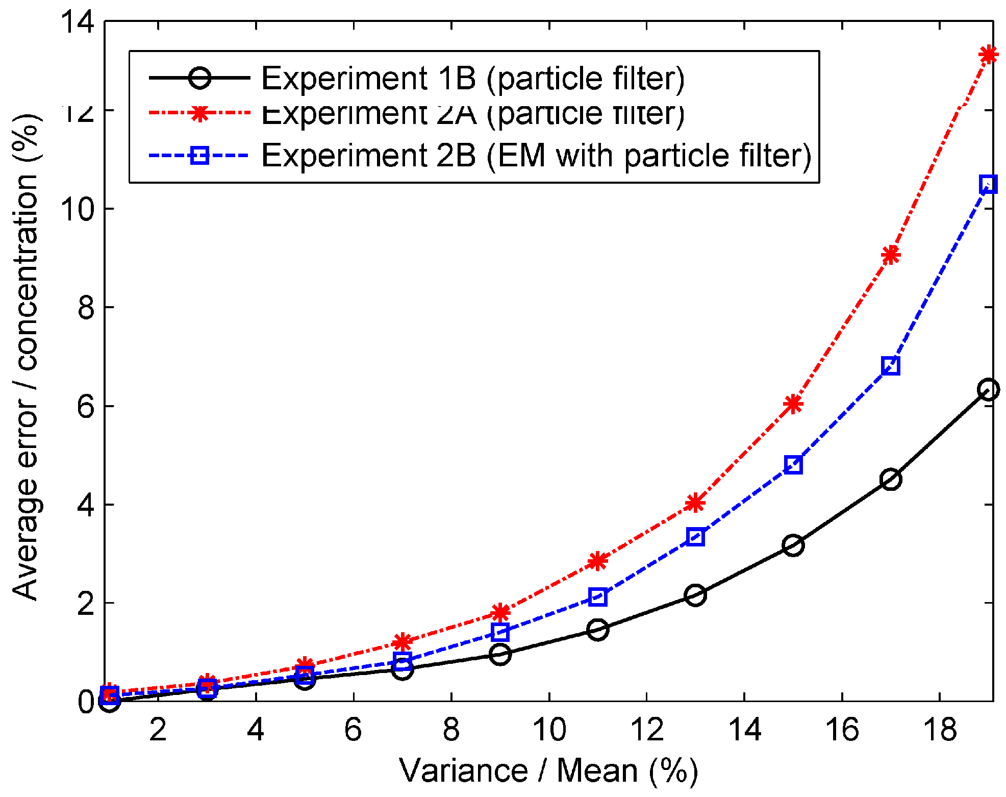
Figure 12.
The percentage errors with different amplitudes of relative variance at some time steps: (a) the percentage error at 30 min; (b) the percentage error at 30 min.
Figure 12.
The percentage errors with different amplitudes of relative variance at some time steps: (a) the percentage error at 30 min; (b) the percentage error at 30 min.

Table 1.
The design of experiments.
| Case | Experiment Name | Group | Method | Note |
|---|---|---|---|---|
| The release rate is known | Experiment 1 | Experiment 1A | Gaussian plume model | Control group: compared to Experiment 1B |
| Experiment 1B | Gaussian plume model & particle filter | Treatment group: test the particle filter | ||
| The release rate is unknown | Experiment 2 | Experiment 2A | Gaussian plume model & particle filter | Treatment group: test the particle filter |
| Experiment 2B | Gaussian plume model & EM with particle filter | Treatment group: test the EM algorithm with particle filter |
Table 2.
Values of state parameters under different atmospheric conditions according to Vogt.
| Atmospheric Stability Class | Coefficients of Dispersion | |||
|---|---|---|---|---|
| a | b | c | d | |
| A | 0.23 | 1.00 | 0.10 | 1.16 |
| B | 0.23 | 0.97 | 0.16 | 1.02 |
| C | 0.22 | 0.94 | 0.25 | 0.89 |
| D | 0.22 | 0.91 | 0.40 | 0.76 |
| E | 1.69 | 0.62 | 0.16 | 0.81 |
| F | 5.38 | 0.58 | 0.40 | 0.62 |
Table 3.
Some key values of state parameters in the “real” dispersions.
| Time (min) | “Real” Dispersion of Experiment 1 | “Real” Dispersion of Experiment 2 | ||||||
|---|---|---|---|---|---|---|---|---|
| a | b | c | d | a | b | c | d | |
| 0 | 0.23 | 1.00 | 0.10 | 1.16 | 0.23 | 1.00 | 0.10 | 1.16 |
| 40 | 0.23 | 0.97 | 0.16 | 1.02 | 0.23 | 0.985 | 0.13 | 1.09 |
| 80 | 0.22 | 0.94 | 0.25 | 0.89 | 0.23 | 0.97 | 0.16 | 1.02 |
| 120 | 0.22 | 0.91 | 0.40 | 0.76 | 0.225 | 0.955 | 0.205 | 0.955 |
Table 4.
The accuracy and total running time of the proposed data assimilation methods.
| Method | RMSE of All Predictions (mg/m3) | Percentage Error (%) | Total Running Time (s) |
|---|---|---|---|
| Particle filter | 0.011471 | 4.56 | 7.68 |
| EM algorithm with particle filter | 0.0059958 | 2.71 | 87.34 |
© 2017 by the authors. Licensee MDPI, Basel, Switzerland. This article is an open access article distributed under the terms and conditions of the Creative Commons Attribution (CC BY) license (http://creativecommons.org/licenses/by/4.0/).
Share and Cite
MDPI and ACS Style
Wang, R.; Chen, B.; Qiu, S.; Zhu, Z.; Qiu, X. Data Assimilation in Air Contaminant Dispersion Using a Particle Filter and Expectation-Maximization Algorithm. Atmosphere 2017, 8, 170. https://doi.org/10.3390/atmos8090170
AMA Style
Wang R, Chen B, Qiu S, Zhu Z, Qiu X. Data Assimilation in Air Contaminant Dispersion Using a Particle Filter and Expectation-Maximization Algorithm. Atmosphere. 2017; 8(9):170. https://doi.org/10.3390/atmos8090170
Chicago/Turabian StyleWang, Rongxiao, Bin Chen, Sihang Qiu, Zhengqiu Zhu, and Xiaogang Qiu. 2017. "Data Assimilation in Air Contaminant Dispersion Using a Particle Filter and Expectation-Maximization Algorithm" Atmosphere 8, no. 9: 170. https://doi.org/10.3390/atmos8090170
Note that from the first issue of 2016, this journal uses article numbers instead of page numbers. See further details here.