The Impact of Tipuana tipu Species on Local Human Thermal Comfort Thresholds in Different Urban Canyon Cases in Mediterranean Climates: Lisbon, Portugal

Abstract

Based upon the case of Lisbon, this article examined the in-situ effects of vegetation upon pedestrian thermal comfort levels. Focussing specifically upon the historic quarter that often witnesses the highest T_amb values and Urban Heat Island (UHI) intensities during the summer, the most common urban canyon cases (UCCs) were modelled, along with one of the most commonly used vegetative semi-deciduous species found in the city, Tipuana tipu. Based upon a reference point (RP) system, the assessments were undertaken through the use of a new version of the SkyHelios model, local obtained G_rad values, and the modified physiologically equivalent temperature (mPET) index calculated through the human-biometeorological model RayMan. The study identified the in-situ thermo-physiological influences of Tipuana tipu during different periods of the year: (1) during the summer, which revealed considerable reductions of PET/mPET of up to 15.6 °C/11.6 °C during a very hot day (where daily maximum T_amb surpassed 35 °C); and (2) during the winter, which revealed the risks of oversharing as a result of the species keeping its foliage during the winter with reductions of PET/mPET of up to 2.7 °C/2.6 °C. Furthermore, the study utilised the climate tourism/transfer information scheme (CTIS) to categorise and facilitate the interpretation of the results.

1. Introduction

Currently, and within existing cities, particularly those concomitant to Mediterranean climates with hot–dry summers and classified with a Köppen Geiger (KG) of ‘Csa’, the importance of local human thermo-physiological thresholds is gaining new weight for local urban design and planning. Still, and often within southern Europe, many cities habitually present a noteworthy absence of climatological data/know-how that could prove useful for local decision making and design within the urban public realm [1].

As a result, and within the context of Lisbon, there have been a substantial amount of studies that have provided valuable contributions towards the comprehension of the overall bioclimatic conditions within its public realm [2,3], UHI intensities [4,5], and integration with planning policy [6,7]. Moreover, and given the progress of the climate change adaptation agenda, studies specifically pertaining to impacts within Lisbon have also been undertaken [8,9,10].

Within the international arena, including within other cities located in other KG classifications, the influences of urban vegetation have already been debated within existing review studies [11,12,13,14]. Within such studies, the benefits of vegetation upon the urban public realm were reviewed, including their capacity to regulate urban ambient temperature (T_amb), and UHI effects. In addition, the scientific community has also endeavoured to expand upon the known in-situ effects of vegetation, including their respective thermo-physiological influences upon pedestrians. Within this line of study, the particular influences of tree species have also been identified within different urban conditions [15,16,17,18,19,20]. It is also worth noting that, within studies which identified bioclimatic conditions/opportunities within different default urban canyon cases (UCCs) (both symmetrical and asymmetrical), the thermo-physiological benefits from vegetation were also mentioned, namely by (i) Ali-Toudert and Mayer [21] in Ghardaia, Algeria (with KG of ‘Bwh’); (ii) Ketterer and Matzarakis [22] in Stuttgart, Germany (with KG of ‘Cfa’); Qaid and Ossen [23] in Putrajaya, Malaysia (with KG of ‘Af’); (iii) Morakinyo and Lam [24] in Hong Kong (with KG of ‘Cwa’); (iv) Algeciras, Consuegra [25] and Algeciras, Tablada [26] in Camagüey, Cuba (with KG of ‘Aw’); and lastly, (v) Nouri, Costa [27] in Lisbon, Portugal (with KG of ‘Csa’).

Notwithstanding, and as suggested by Kong, Lau, et al. [28] within the scientific community, there are still a greater amount of studies which have focussed upon T_amb variations rather than thermo-physiological impacts as a result of local vegetation. Concomitant with this perspective, this article is centred upon the importance of going beyond sole climatic characteristics, and aims to add to the existing studies which identify the significance of considering ‘in-situ’ thermo-physiological influences resultant of urban vegetation.

In line with this objective, this study (i) utilises a new version of the SkyHelios model [29,30] as a new means to address microclimatic characteristics (namely Wind (V) speed); and, (ii) examines and applies new modified thermo-physiological indices [31] to conduct more accurate evaluations of thermal comfort conditions during different periods of the year. Such methods are applied to the case of Lisbon to identify how one of the most commonly-found shading trees within the city (i.e., Tipuana tipu) can influence the in-situ bioclimate conditions within symmetrical urban UCCs which are typically located within the city’s historical district. The results of the study indicate (1) how simulations can be united with field measurements to compare and adapt climatic data from the local meteorological station; (2) the in-situ thermo-physiological effects that a common shading tree can have upon pedestrians during the summer and winter periods in areas prone to higher thermal stimuli, particularly during the summer; and lastly, (3) how such outcomes can ease the transition and ‘shared language’ [1] between the fields of urban climatology and local urban design/planning.

2. Experiments

2.1. Site

Located on the western coast of Portugal at 38°42′ N and 9°8′ W, Lisbon has a KG classification of ‘Csa’, which constitutes a Mediterranean climate with dry and hot summers [32]. Accordingly, and as identified by studies conducted by Miranda [33] and Calheiros [34], the urban microclimatic conditions present annual periods in which outdoor thermal comfort thresholds can be strained as a result of numerous of climatic occurrences, namely (i) between 10 and 20 days where daily maximum T_amb surpasses 35 °C; (ii) an occurrence of between 100 and 120 ‘summer days’ where daily maximum T_amb exceeds 25 °C; and additionally (iii) frequent occurrences of heat waves, where daily maximum T_amb exceeds that of 32 °C for various periods of successive days.

As identified in the study conducted by Alcoforado, Andrade [1], both North and Northwest wind directions are the most common throughout the year, particularly during the summer. This being said, due to the proximity to the Tagus, Lopes [35] identified that estuarine breezes reach adjacent urban areas on 30% of the late mornings and early afternoons during the summer. This study focuses predominantly upon the historical quarter of ‘Baixa Chiado’, which due to its general morphological composition has been identified to frequently witness the highest UHI intensities [2] and highest temperatures during the summer [6].

2.2. Data

To retrieve the base climatic data for the study, meteorological recordings were attained from the World Meteorological Organisation weather station with the Index N°08535, located within Lisbon with the latitude of 38°43′ N, 9°9′ W, and an altitude of 77 m. As with similar existing studies [1,19,25,31,36,37,38,39], the extracted data was converted into a variation of the thermo-physiological index, physiologically equivalent temperature (PET) [40,41,42]. The respective index was used due to the (i) feasibility of being calibrated upon easily obtainable microclimatic parameters; and (ii) base measuring unit being °C, which facilitates its comprehension by professionals such as urban planners and designers when approaching climatological facets.

Before considering the influences of UCCs and vegetation, an initial analysis was established to determine general diurnal thermal conditions during different climatological circumstances, i.e., during the summer and winter within the city (

Table 1. Average and diurnal (3rd of July and 16th of December) climatic data obtained from weather station (Index N°08535; Okt: oktas).

Time	$\overline{\mathit{J}\mathit{u}\mathit{l}\mathit{y}}$				3rd July				$\overline{\mathit{D}\mathit{e}\mathit{c}\mathit{e}\mathit{m}\mathit{b}\mathit{e}\mathit{r}}$				16th December
	Tamb	RH	V1.1	Okt	Tamb	RH	V1.1	Okt	Tamb	RH	V1.1	Okt	Tamb	RH	V1.1	Okt
	C°	%	m/s		C°	%	m/s		C°	%	m/s		C°	%	m/s
09:00	24.5	56.7	1.8	2.0	26.4	54.2	2.1	0.0	10.5	86.0	1.7	3.7	10.0	79.9	2.1	7.0
10:00	25.9	51.9	1.8	1.7	26.9	58.6	1.6	0.0	11.6	82.2	2.0	3.6	8.9	89.1	3.6	7.0
11:00	27.6	46.7	1.9	1.2	31.7	44.4	1.0	0.0	12.7	76.6	1.9	3.5	9.2	87.3	3.6	7.0
12:00	28.8	43.7	1.9	1.1	33.0	39.5	1.0	0.0	13.9	72.9	1.7	3.5	10.2	77.8	3.0	6.0
13:00	29.4	41.4	2.3	1.1	35.0	35.1	1.6	0.0	14.7	69.6	1.7	3.5	9.8	81.6	4.1	6.0
14:00	29.7	41.4	2.5	1.1	34.7	35.7	1.6	0.0	15.1	68.3	1.7	3.7	12.2	72.5	3.6	6.0
15:00	29.4	41.6	2.8	1.1	35.9	32.5	1.0	0.0	14.8	70.5	1.6	3.8	11.5	75.4	3.1	7.0
16:00	27.9	46.1	2.9	0.9	34.3	37.4	2.0	0.0	14.7	71.3	1.5	3.7	12.4	72.0	3.6	7.0
17:00	27.3	47.4	2.9	0.9	32.9	39.9	2.6	0.0	14.3	73.6	1.5	3.6	12.0	68.1	4.1	7.0
18:00	26.5	48.6	2.7	0.9	31.2	40.7	2.6	0.0	13.7	76.7	1.5	3.6	11.6	68.9	4.2	7.0

). Such an approach enabled a ‘base understanding’ of Lisbon’s thermo-physiological conditions as presented by the weather station.

In order to carry out this initial assessment, the RayMan Pro^© model [43,44] was used to process the following retrieved parameters: T_amb, relative humidity (RH), total cloud oktas (Okt), and V₁₀. In addition to these climatological aspects, the calibration of the RayMan model was constructed upon the default standing ‘standardised man’; i.e., a height of 1.75 m, weight of 75 kg, aged 35, with a clothing 0.9 clo, and an internal heat production of 80 w [40,41]. In order to account for the deceleration effect of ‘urban roughness’ upon wind speeds obtained from the meteorological station [45], the values were adapted to permit the estimation of V values upon the gravity centre of the human body. As a result, V₁₀ values were interpreted to a height of 1.1 m (henceforth expressed as V_1.1) by using the formula presented by Kuttler [46] (Equation (1)). Given Lisbon’s denser downtown district with frequent open spaces, and similar to the morphological layout/compositions examined within comparable bioclimatic studies in Barcelona [38] and within the historical district of Lisbon [27], the study applied the following calibrations to the formula: z₀ = 1.00 m, and α = 0.35.

$${\mathrm{V}}_{1.1}=V_h\times {\left(\frac{1.1}{h}\right)}^{\alpha }\alpha =0.12\times z_0+0.18$$

(1)

where V_h is the m/s at a height of h (10 m), α is an empirical exponent, depending upon urban surface roughness, and z₀ is the corresponding roughness length.

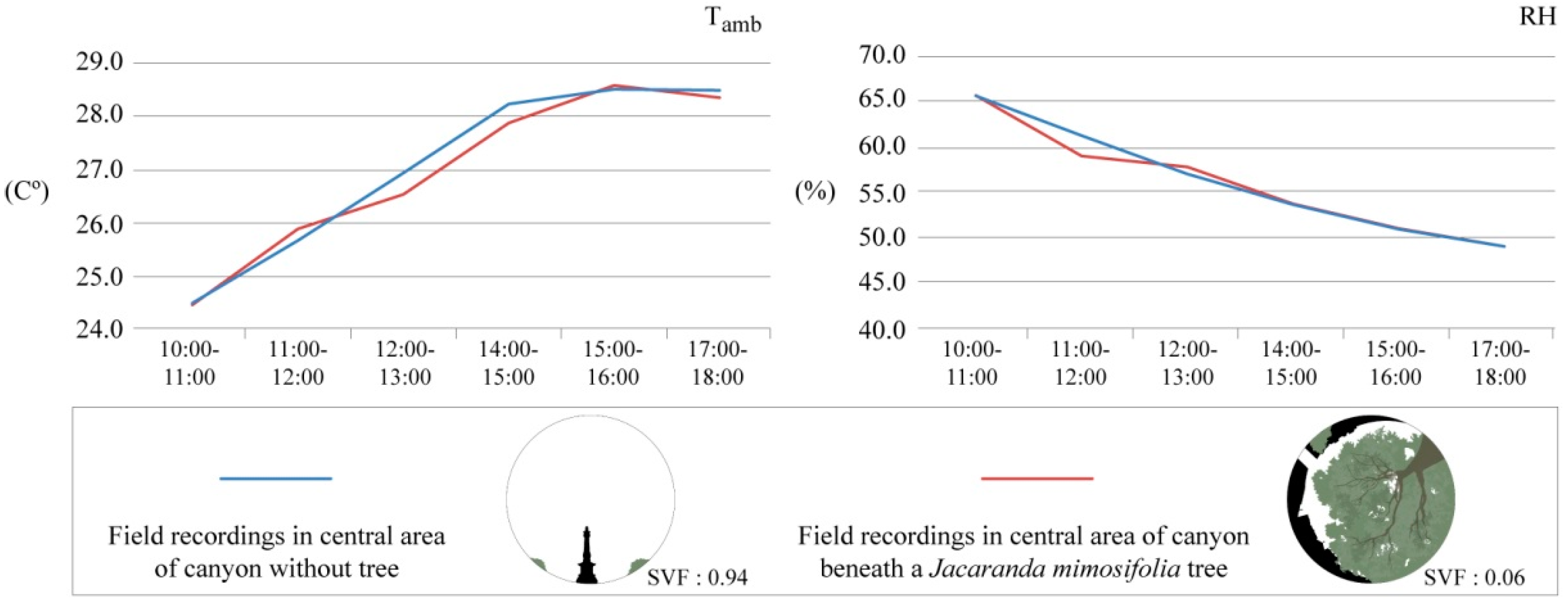
At a later stage in the study, another variable tuning was considered when addressing the ‘in-situ’ effects of vegetation upon pedestrian comfort as a result of evapotranspiration. As identified by the early studies of Oke [47], McPherson [48], and Brown and Gillespie [49], T_amb and RH are usually not meaningfully modified by landscape elements such as trees since the encircling atmosphere quickly dissipates any such in-situ oscillations. 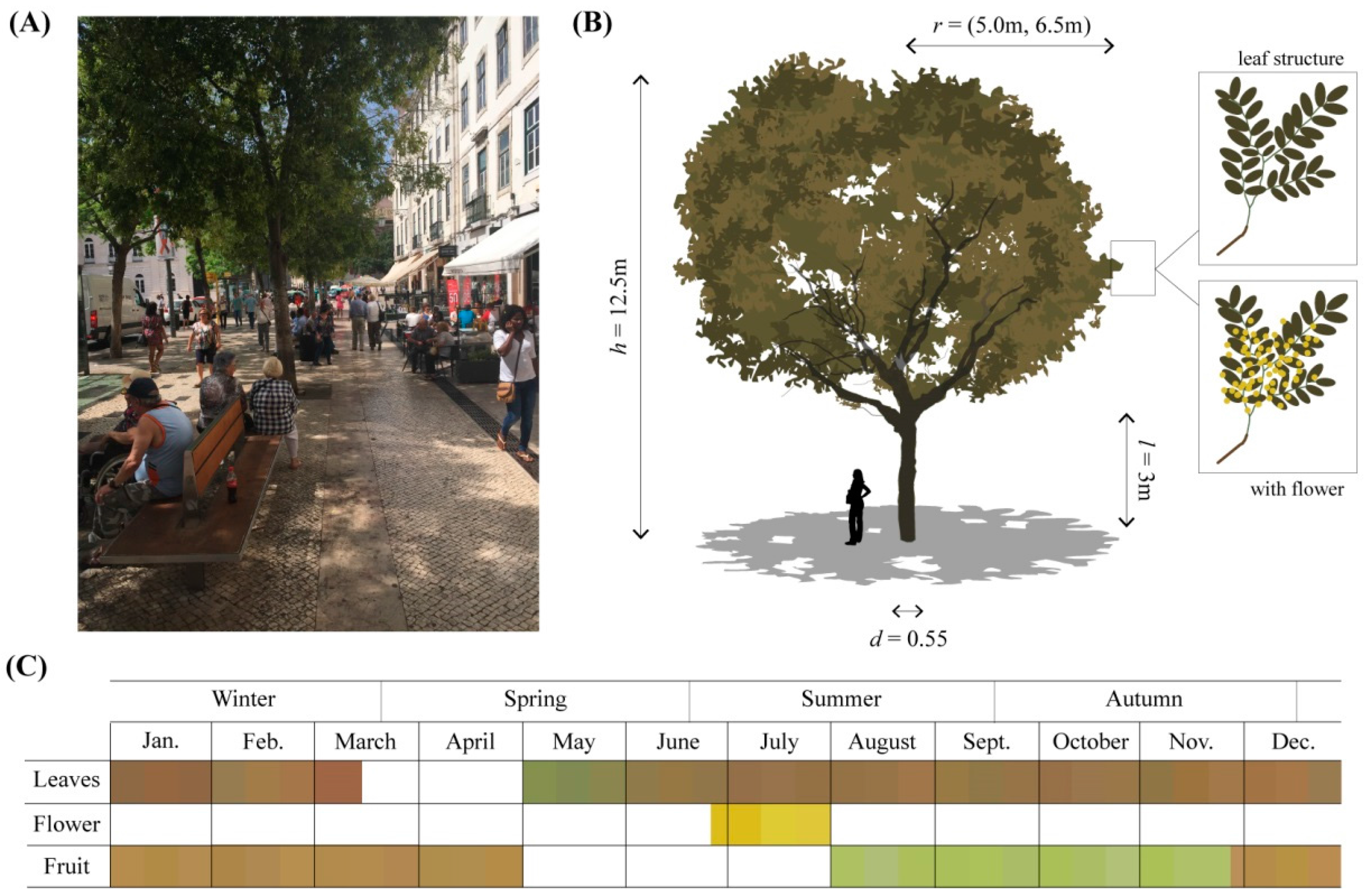Such results were also obtained by later studies [19,50,51,52,53] who identified such limitations resulting from evapotranspiration effects, particularly from single trees. Moreover, such outcomes were also obtained by a recent study conducted within one of the widest public spaces located in Lisbon’s historical centre. Carried out in July 2015, and as shown in Figure 1 the limited effects of evapotranspiration beneath the crown were also verified.

As a result, the lower impact that evapotranspiration could generate upon comfort conditions at pedestrian height was not considered in this particularly study. Instead, the assessments were predominantly based upon evaluating the in-sit’ impacts of a specific tree species beneath its crown, or in other words “the cool feeling people experience as a result of a reduction in radiation” [15]. Although such information has grown in recent years (as exemplified by numerous studies mentioned in this study), the authors argue that there is still a need to build upon estimations of radiation modifications as a result of vegetative deflection as suggested by Brown and Cherkezoff [55]. As a result, such outputs should continue to build upon the growing comprehension of vegetation influences upon microclimatic characteristics at the pedestrian level [56].

Therefore, supplementary data modifications/calibrations were applied to assess the specific thermo-physiological in-situ effects of Tipuana tipu upon pedestrian comfort levels. In addition to the preliminary climatic variables, global radiation (G_rad) retrieved by the authors were used to supplement the radiation flux assessments. These values were obtained through field surveys through the use of the handheld apparatus KKMOON SM206, with an accuracy of ±10 and a resolution of 0.1 W/m². Similar to the approach carried out by Nouri and Costa [54], such measurements were established to obtain hourly oscillations of G_rad (i) in specific locations of different UCCs; and (ii) beneath vegetative canopies to identify the amount radiation that was diluted by the vegetative crown mass. Such an approach enabled solar attenuation radiation levels to be determined specifically beneath the tree crowns, and later introduced within the biometeorological model.

2.3. Applied Methodology and Structure

The modelling, refinement, and representation of the UCC assessments were processed through a three-step approach. Firstly, a new version of the SkyHelios model⁽ⁱ⁾ [29] was used in order to assess the microclimatic conditions and implications upon the introduced parameters with respect to the urban morphologies. As presented by Fröhlich [30], the model has been developed to analyse the spatial dimension of a specific microclimate. The short runtime and wide range of support input formats, as well as the capability of dealing with different projected coordinate systems permit the applicability of the model to evaluate the comparison of different UCCs, tree compositions and their effect on thermal biometeorology. In processing terms, the new SkyHelios model essentially follows a similar approach to that of the Rayman model, but it has the additional feature of also considering the spatial dimension of the parameters. As a result, SkyHelios makes use of the graphic processor for computing the sky view factor (SVF) [29]. Based upon the SVF, the radiation fluxes can be determined for any location within the respective model area, and summarised as mean radiant temperature (T_mrt). As defined by Oke [47], the SVF is the fraction of the visible sky seen from a specified point. Within the software module, the first operation is the rendering of a fisheye image for that stipulated location, and secondly, the SVF is determined by distinguishing transparent and coloured pixels within the generated image. Similar to real environments, the fisheye image is a half-sphere, and not all of the pixels should have the same influence upon SVF. Therefore, a dimensionless weighting factor represented as ωproj (Equation (2)) is utilised to consider the projections that adjusts the impact of a pixel by the sine of the zenith angle φ (◦).

$$\omega proj=\sin \left(\phi \right)\times {\left(\frac{\phi }{90°}\right)}^{-1}$$

(2)

This results in a spherical SVF, whereby if a planner SVF is desired, another correction by ωplanar (again dimensionless) needs to be performed (Equation (3)). Such a modification increases the impact of objects close to the ground by the cosine of the azimuth angle (counted from the ground to the top).

$$\omega planar=\omega proj\times \cos \left(\phi \right)$$

(3)

Furthermore, a three-dimensional diagnostic wind model was integrated within the updated version in order to provide estimations of ‘in-situ’ V measurements, which as discussed can differ significantly from those presented by the meteorological station. Such a model was based upon the approach conducted by Röckle [57], but, and as discussed by Fröhlich [30], with updated parameterizations, namely (i) an improved upwind cavity as discussed in Bagal, Pardyjak [58]; and (ii) an improved description of street canyon vortices as described in Singh, Hansen [59]. As a result, the SkyHelios model enables the identification of spatially-resolved V and associated direction. The wind field calculated by the given functions most likely contains a certain degree of divergence. Assuming incompressible air, such a divergence has to be minimized in order to get a valid wind field. In mathematical terms, this is performed by minimizing the functional for the scalar H (Equation (4)).

$$\mathrm{H}\left(u,v,w\right)=\iiint (b_{\mathrm{h}}^2{\left(u-u^0\right)}^2+b_{\mathrm{h}}^2{\left(v-v^0\right)}^2+b_{\mathrm{v}}^2{\left(w-w^0\right)}^2)dxdydz$$

(4)

As shown in Equation (4) b_h and b_v are horizontal stability factors in s/m; u, v and w are the stream components in m/s, u⁰, v⁰ and w⁰ are representative of the initial stream components in m/s while dx, dy and dz are the grid spacing in metres. Due to this integration, the model is capable of estimating thermal indices Perceived Temperature (PT) [60], Universal Thermal Comfort Index (UTCI) [61], and PET that are spatially resolved at high resolutions (e.g., 1 × 1 m).

The second step was orientated at processing the results through the updated version of the RayMan model⁽ⁱⁱ⁾ in order to interpret them into the modified physiologically equivalent temperature (mPET) as discussed in Chen and Matzarakis [31]. As presented in their study, the predominant differences of the mPET index are the integrated thermoregulation model (based upon a multiple-segment model), and the clothing model which relays a more accurate analysis of the human bio-heat transfer mechanism. For this reason, the initial examination of the diurnal conditions both during the summer and winter conditions were thus presented in both PET and mPET; to firstly examine such differences identified by Chen and Matzarakis [31], and secondly, present more accurate evaluations of the human thermal comfort conditions examined later in the study.

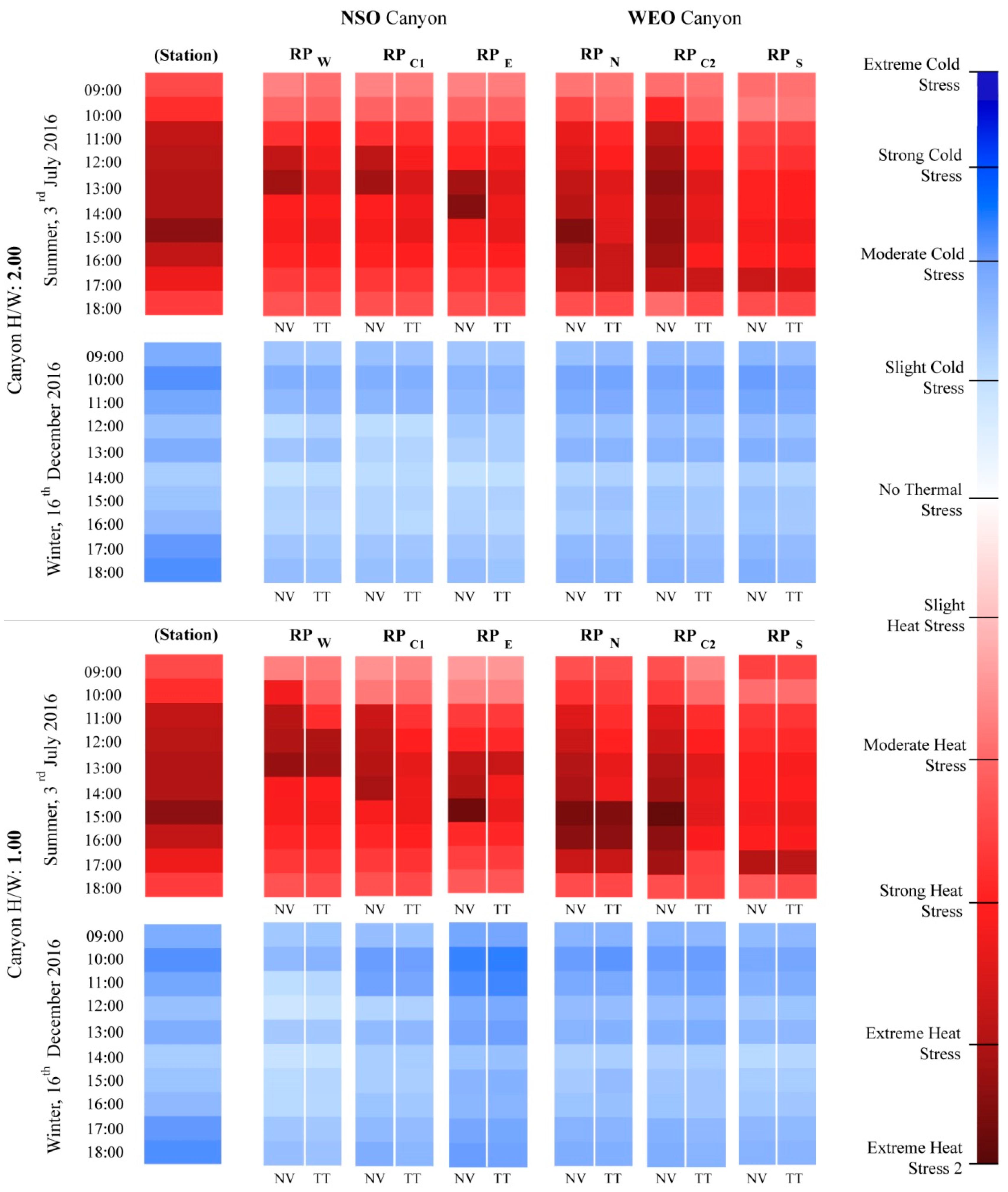
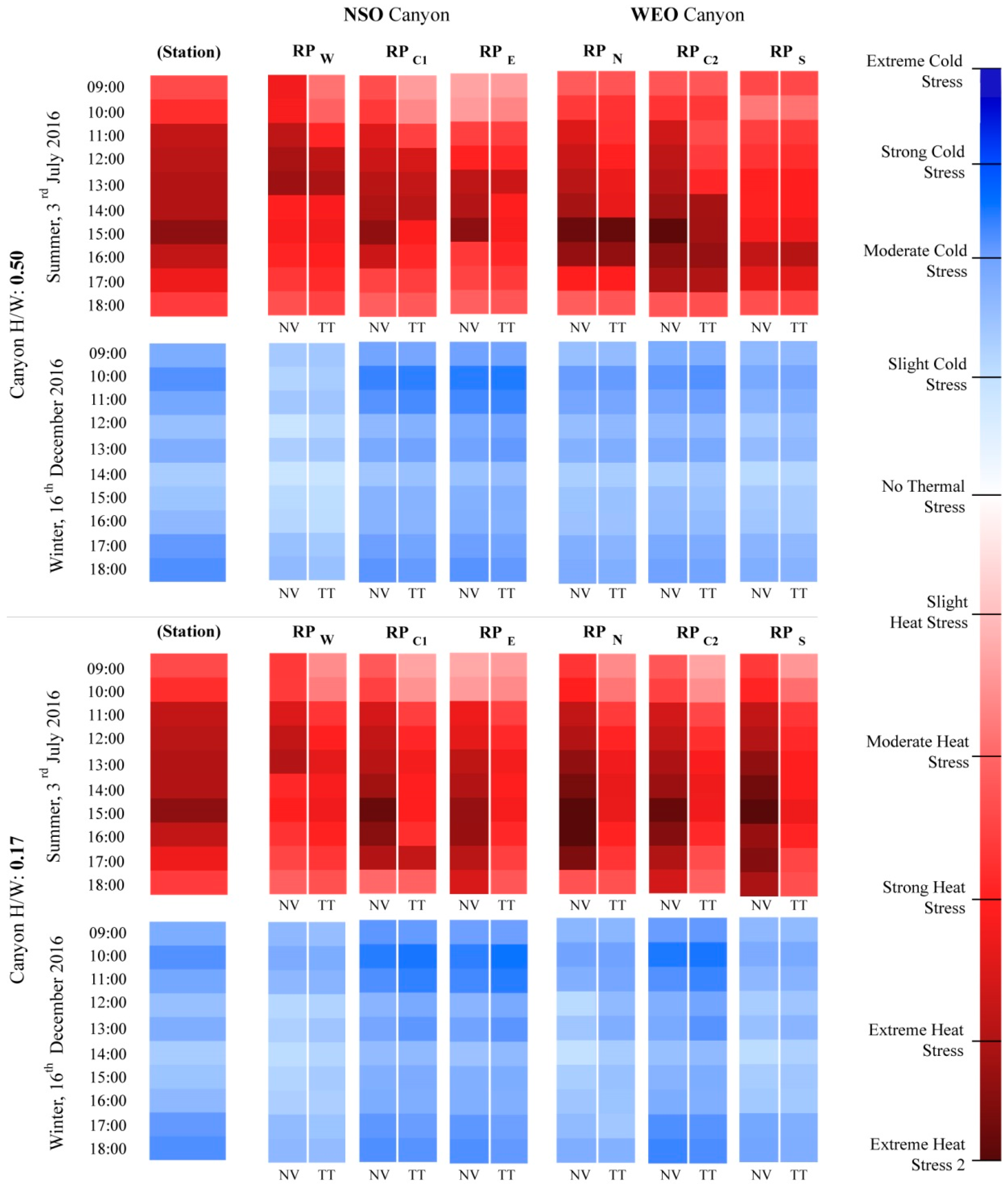
The third step of the study was to ensure that the study outputs were communicated in a way to facilitate their comprehension by non-experts in the subjects linked to climatology. As a result, the obtained results were processed with the climate tourism/transfer information scheme⁽ⁱⁱⁱ⁾ (CTIS) [62]. Such means of communication have been growing within the scientific community in similar climatic studies [31,38,63,64,65].

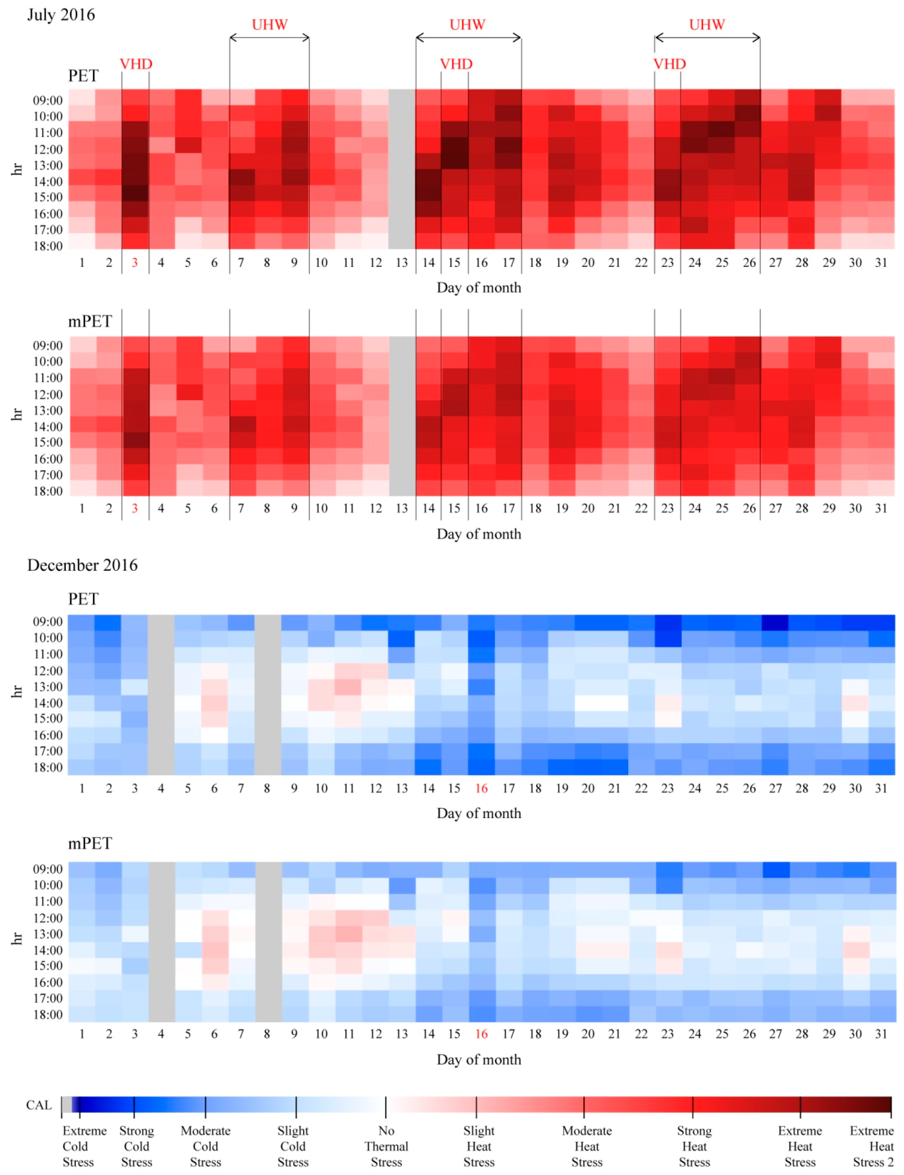
2.3.1. Identification of Bioclimatic Conditions During Summer/Winter Periods

As discussed, the first stage was to identify the general bioclimatic conditions (i.e., PET and mPET values) retrieved from the specified weather station. As a result of this exercise, not only was it possible to identify how physiological stress (PS) grades vary during different times of the year, but moreover to identify the days on which the simulations would be based. Based upon the configuration of the meteorological station, since the total Okt values were only recorded at 09:00, 12:00, and 15:00, it was necessary to approximate values for the remaining hours between 09:00 and 18:00. Such an approximation was undertaken by (i) the delineation of the mid-range values between the three daily recordings; and, in addition, (ii) taking into account the qualitative meteorological descriptions provided by the station. Such inputs were accompanied by the introduced T_amb, RH, and V_1.1 diurnal recordings for the months of July and December, each representative of the hottest and coldest annual conditions for 2016 found in Lisbon (Table 1). Furthermore, and at this stage of the study, the applied SVF value was calibrated at 1.00 (or 100%) which would reproduce an assessment with total exposure to solar radiation. Once the PET and mPET values were processed, the comparative chart presented by Matzarakis, Mayer [42] was used in order to categorise the obtained temperature values into specific PS levels, shown in

Table 2. Ranges of the thermal index physiologically equivalent temperature (PET) for different grades of physiological stress (PS) on human beings; internal heat production: 80 W, heat transfer resistance of the clothing: 0.9 clo according to [66] | Source: Adapted from, [42].

PET	PS
<4 °C	Extreme Cold Stress
4–8	Strong Cold Stress
8–13	Moderate Cold Stress
13–18	Slight Cold Stress
18–23	No Thermal Stress
23–29	Slight Heat Stress
29–35	Moderate Heat Stress
35–41	Strong Heat Stress
>41	Extreme Heat Stress

.

Once the boundaries for each temperature range were stipulated, it was possible to input such margins into CTIS to facilitate the representation of the diurnal modifications of PS during the months of July and December. Such methods of representation have already been used in similar bioclimatic studies [31,38,63,64,65] which also aimed at facilitating the comprehension of the obtained thermo-physiological results.

2.3.2. Defining Tipuana tipu Characteristics and Layout

The Tipuana tipu species originates from the region adjacent to the Tipuani River in Bolivia, and is also known for its lineages from both Brazil and Argentina. Given the right conditions, the species can reach considerable sizes, and presents a dark trunk, twisted branches, and a densely vegetated round crown. Resulting from the ‘Csa’ climate, the equally ornamental and rustic species are particularly compatible with Lisbon’s climate. Consequently, they are one of the most commonly used deciduous species [67], with approximately 1900 examples within the city [68,69]. In a few locations, a particular few have been listed as ‘public interest’ due to their considerable age and size as exemplified in ‘Cais Sodré’, ‘São Bento’ Plaza, and the ‘Nove de Abril’ Park, registering ages of 100, 80, and 128, respectively. Recognised as an effective urban shading tree specifically within Mediterranean climates [17,54,67,69,70,71,72] it is also frequently mixed with other species within Lisbon. Such circumstances can be exemplified by a mixture with other identified ‘shading trees’ such as Jacaranda mimosifolia within the urban garden of ‘Santos’ and the public plaza of ‘Rossio’ within the historical quarter.

The example of the latter is illustrated in Figure 2A, which shows a lined sidewalk seating area beneath the vegetative crowns of a linear plantation of Tipuana tipu with a parallel row of Jacaranda mimosifolia on the edge of the sidewalk. Common to sidewalk plantation typologies as identified by Torre [70], the linear plantation configuration has been identified to effectively attenuate (i) radiation, especially when the tree lines are parallel/close to a building frontage [48,49,73,74]; and (ii) wind patterns that take place perpendicularly to the tree line [70,72,75].

Within urban pavements, the species often present smaller sizes [17,67,72,76] which is often due to inferior soil conditions and embedding methods. Illustrated in Figure 2B, and based upon the aforementioned studies, the dimension of the trees used within the study were calibrated with a height (h) of 12.5 m, vegetative crown radius (r) of 5.0/6.5 m, trunk length (l) of 3 m, and a trunk diameter (d) of 0.55 m. Furthermore, since G_rad values were measured beneath the crowns, parameters such as leaf area index and leaf angle distribution were not required to determine the vegetative density/transmissivity of the tree crown.

Beyond being one of the most commonly used ‘shading’ tree species, and unlike most deciduous species, it also has the particularity of maintaining its foliation both during the summer and winter period. As demonstrated in Figure 2C, and as identified by Viñas, Solanich [72] within the Iberian Peninsula, the only period in which the Tipuana tipu loses its leaves is during the early spring. Accordingly, and given the permanency of its vegetative crown during the winter, it was also possible to assess how the vegetative crown would influence ‘in-situ’ thermal conditions during colder conditions. As identified by early studies [15,49,55,77], it was possible to examine the consequences of reductions of radiation fluxes during the winter; a known essential microclimatic variable with both physiological and psychological connotations to counteract colder conditions during the winter in outdoor urban public spaces [78].

2.3.3. Application and Construction of the SkyHelios Simulations

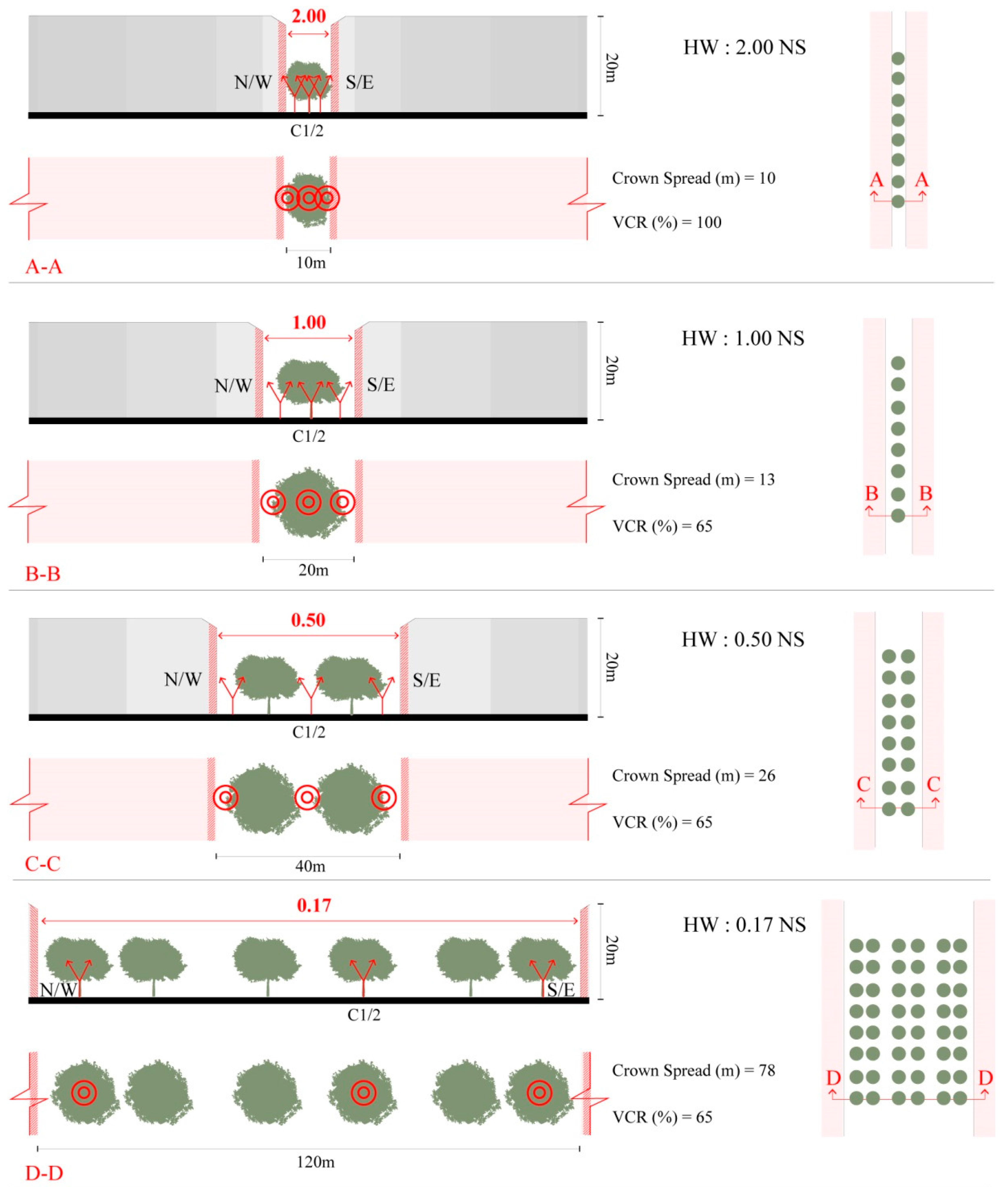
Within the ‘Obstacle’ plugin associated with both the RayMan and the SkyHelios models, various morphological compositions were constructed. Based upon modifying one of the characteristics of the canyons, it was possible to obtain dissimilar height-to-width (HW) ratios which were the most commonly found within Lisbon’s historical district. Accordingly, the canyon height was maintained at 20 m (equating roughly to a building of five stories), and the canyon widths fluctuated between 10, 20, 40, and 120 metres to obtain ‘very high’, ‘high’, ‘medium’, and ‘very low’ UCCs, respectively. Although focused upon a larger scale, a similar approach was applied by Norton, Coutts [79], who categorised broad priority requirements for green infrastructure within different urban canyons. Previously, an UCC with a description of ‘low’ was also initially considered for the study. Such a canyon presented a canyon width of 80 m, and a HW ratio of 0.25, yet based upon a previous study conducted by the authors, it was identified that it presented almost identical thermal conditions to the 0.17 ratio. As the latter presented greater dissimilarities to the higher 0.50 ratio, it was decided to focus upon the four identified UCCs within this specific study as presented in

Table 3. Description and categorisation of utilised urban canyon cases (UCCs) and their respective height, width, and height-to-width (HW) ratio.

UCC Description	Canyon Height	Canyon Width	HW Ratio
‘Very High’	20	10	2.00
‘High’	20	20	1.00
‘Medium’	20	40	0.50
‘Very Low’	20	120	0.17

.

In accordance with the proportional and rigid morphological composition succeeding the reconstruction of Lisbon’s historical district following the great earthquake of 1755, all modelled canyons were symmetrically configured. Although such an approach is frequently ‘presumed’ when approaching H/W ratios, recent microscale bioclimatic studies [23,26] have also produced important results in asymmetrical canyons whilst also addressing urban thermal comfort conditions.

Through the use of the SkyHelios model, the HW_2.00, HW_1.00, HW_0.50, and HW_0.17 were processed under two conditions: (i) without the presence of vegetation; and (ii) with the presence of vegetation. In addition, each canyon was aligned into a north-to-south orientation (NSO) and a west-to-east orientation (WEO) in order to assess the influence of the geo-referenced summer/winter sun path upon the two alignments. The layout of the NSO simulations with the presence of the Tipuana tipu is represented in Figure 3 indicates how, depending upon the UCCs, the tree layouts were structured within each undertaken assessment. Such an adjustment was based upon maintaining a similar amount of vegetative coverage ratio (VCR) throughout the width of each UCC. Within this study, such an indicative value was obtained by applying the straightforward formula as shown in Equation (5).

$$\mathrm{VCR}=\frac{\left(100\times CS\right)}{W}CS=n\times r\times 2$$

(5)

where W is the width of the aspect ratio, CS is the crown spread, n is the number of trees, and r is the radius (5, 6.5).

Although the VCR was based upon determining the amount of vegetation against the width of the canyons, comparable ratios were also utilised within similar studies [17,56,80] who quantified the amount of vegetative biomass within an entire outdoor area. Based upon the discussed parameters in Figure 2B, the dimensions of the introduced trees were calibrated with a diameter of 13 m, with the exception for HW_2.00, which accommodated trees with a lower diameter of 10 m. Such a reduction was undertaken to account for the shorter width of the street, whilst respecting the smaller, yet feasible dimensions of the Tipuana tipu.

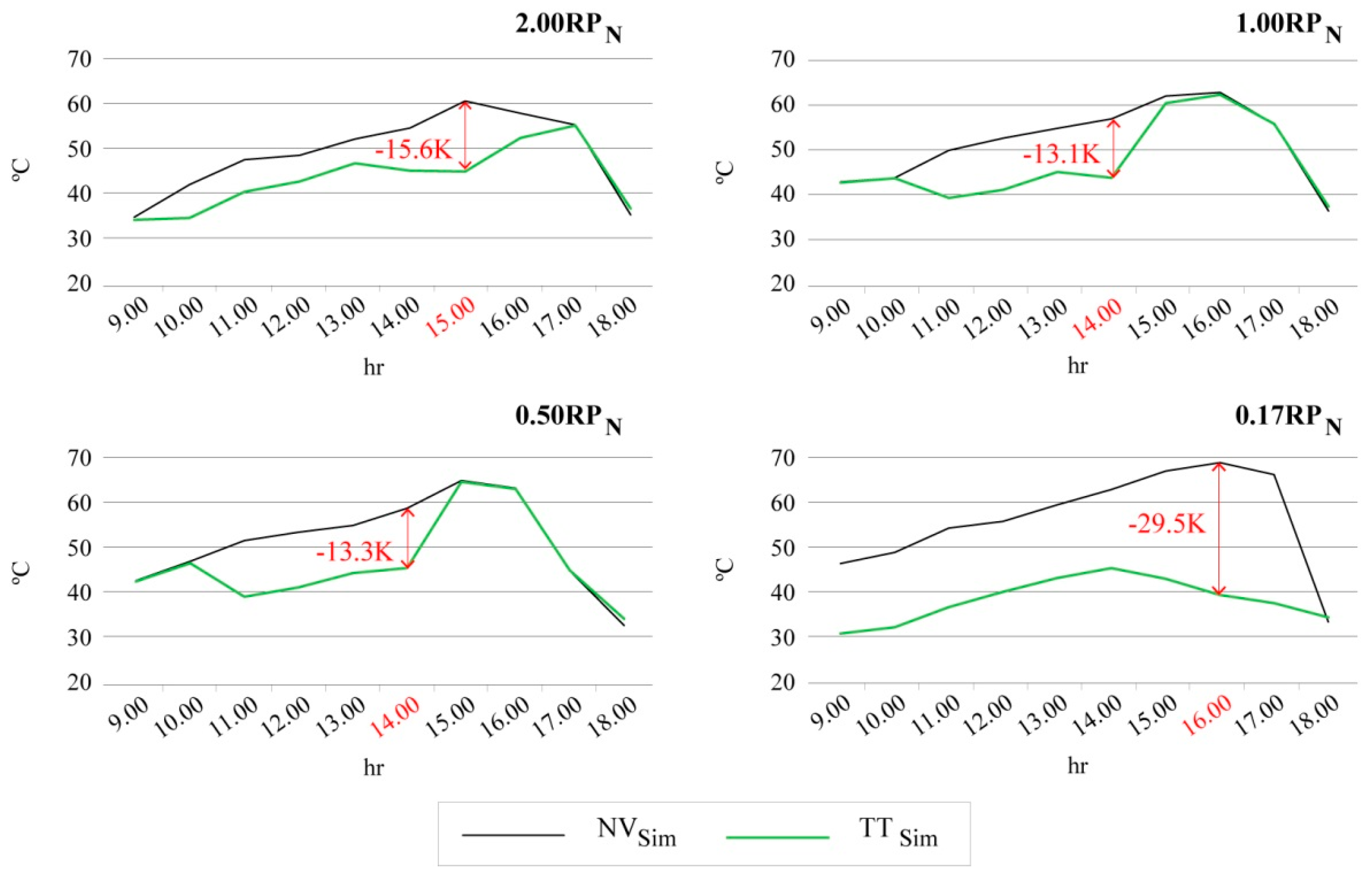
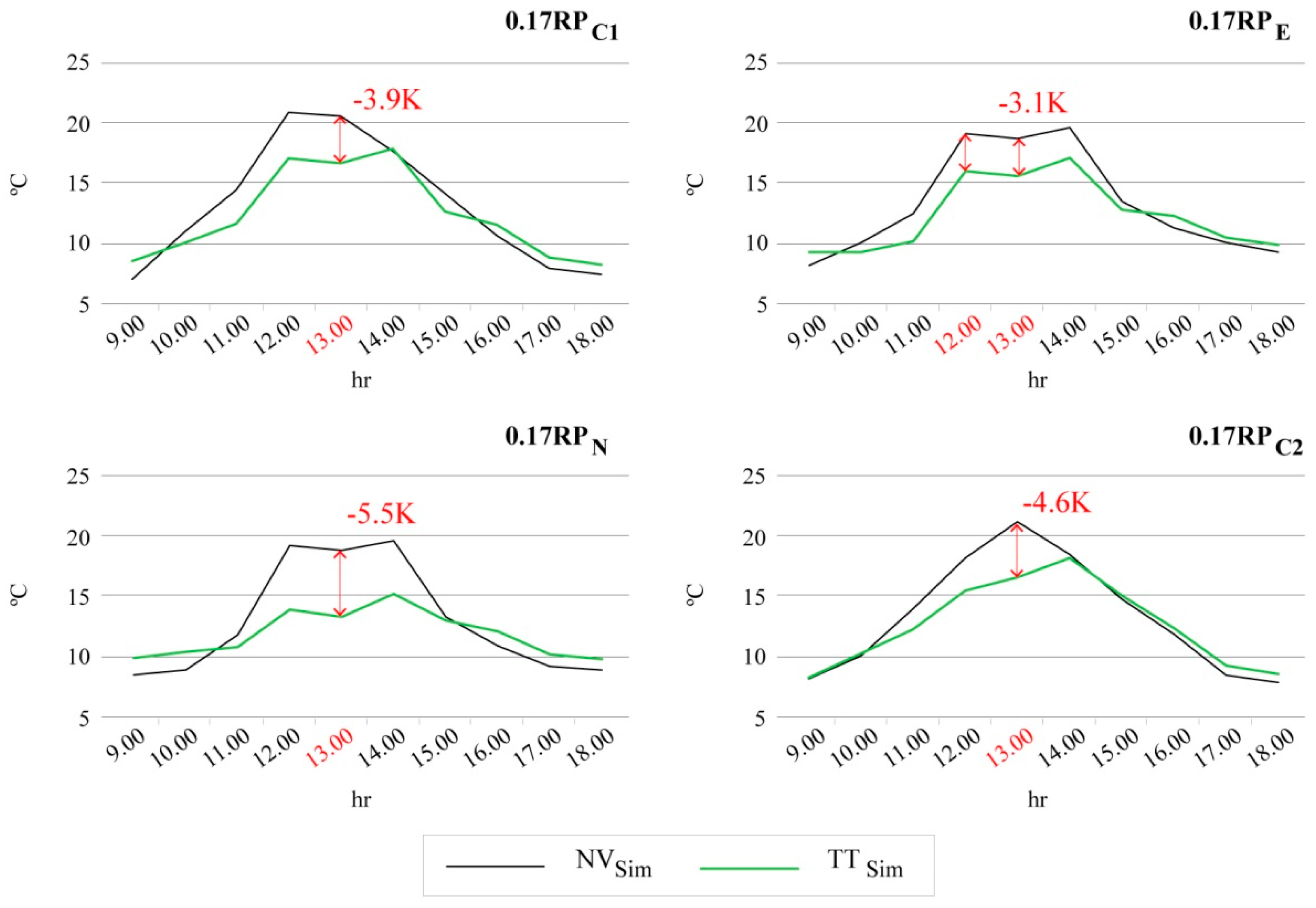
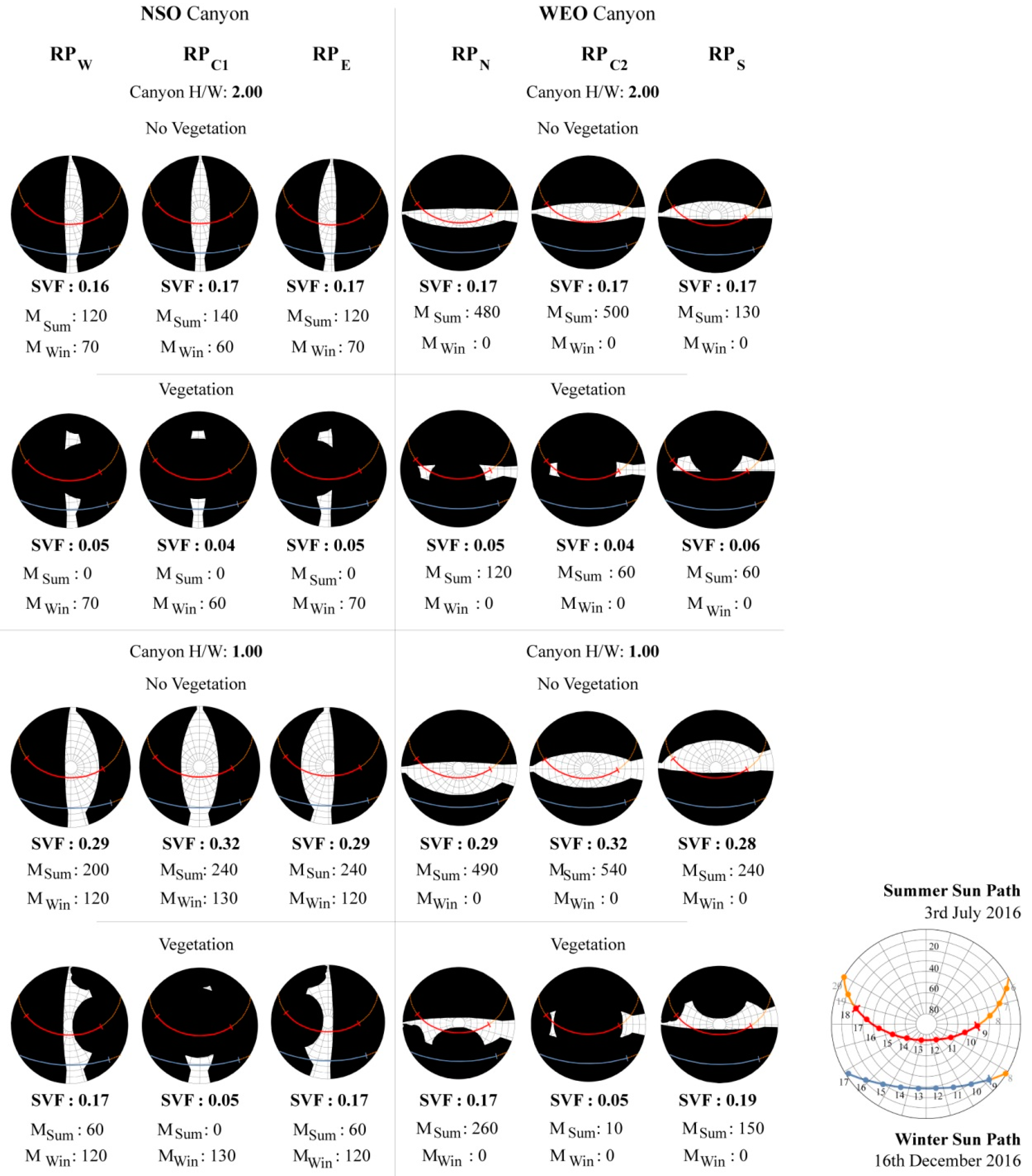
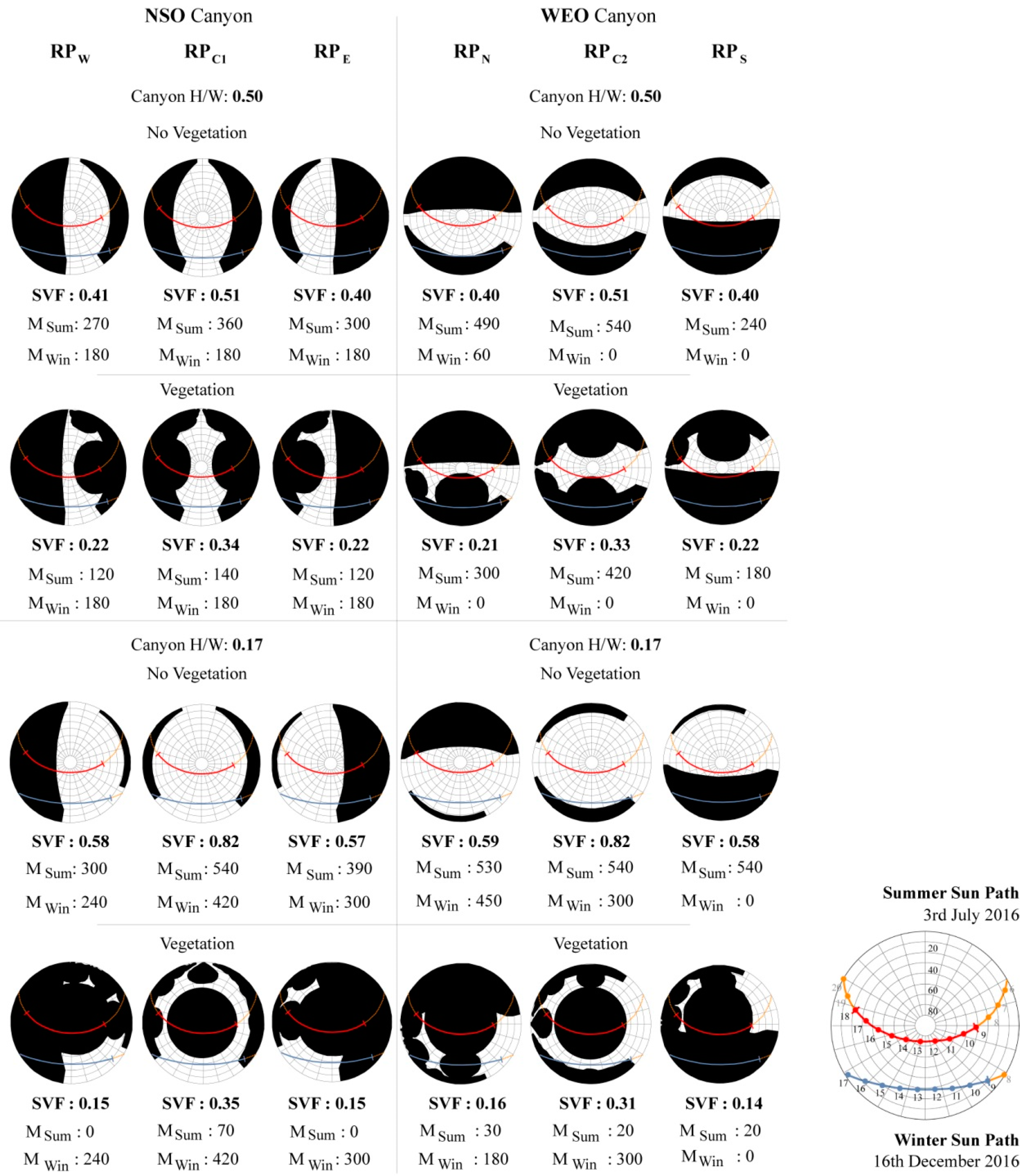
As presented within the study conducted by Lin, Tsai [81], the calculation of SVF within this study was based upon the classic single-point SVF within a specific location in the canyon to obtain a fisheye image at a calibrated height of 1.1 m. Similar to an approach applied by Algeciras, Consuegra [25] both the NSO and WEO accommodated three specific reference points (RPs) which were established to identify the diurnal oscillations of solar radiation. As shown in

Table 4. Stipulation of reference points (RPs) within each of the assessed urban canyon cases (UCCs) based upon single-point sky view factors (SVFs).

SkyHelios RP Stipulation
Region	Lateral 1		Central		Lateral 2
Orientation	NS	WE	NS	WE	NS	WE
Location
Reference Point	(RPW)	(RPN)	(RPC1)	(RPC2)	(RPE)	(RPS)

, the RPs were attributed a specific location within the different UCCs, and their respective coordinates within the SkyHelios model are presented and discussed in

Table 5. Input coordinates and description of reference points (RPs) within each assessed canyon, each with a total length of 200 m.

		SkyHelios Coordinate Input Values								SkyHelios 1.00 Screenshot
UCC°	RP	2.00		1.00		0.50		0.17
		X	Y	X	Y	X	Y	X	Y
N/S	W	47.2	−49.6	42.4	−53.6	34.2	−50.6	46.8	−54.6
	C1	49.9	−49.6	50.1	−53.6	50.1	−51.6	110.5	−54.6
	E	52.9	−49.6	57.3	−53.6	66	−51.6	152.6	−54.6
W/E	N	200.6	−52.8	197.1	−57.1	198.4	−65.8	195.9	−151.7
	C2	200.6	−49.7	197.1	−49.4	198.4	−50.1	195.9	−89.7
	S	200.6	−46.9	197.1	−42.3	198.4	−33.8	195.9	−47.5
HW	Description of RP placement
2.00	Central and lateral RPs were varied little due to the limited width of the canyon
1.00	Central RPs were placed beneath tree crown, while the lateral RPs were situated amid the edge of the tree crown and the lateral façades of the canyon
0.50	Central RPs were placed between the edges of two tree crowns, and the lateral RPs placed between the edge of the tree crown and the lateral façades of the canyon
0.17	Central RPs were slightly offset to be directly beneath a tree crown, and lateral RPs which were also placed beneath the trees located adjacent to the façades of the canyon

. Additionally, and even though canyon length was un-associated to the HW ratio, each was attributed a length of 200 m in order ensure that ‘edges’ of the default canyon would not meaningfully affect the obtained SVF values obtained by the SkyHelios.

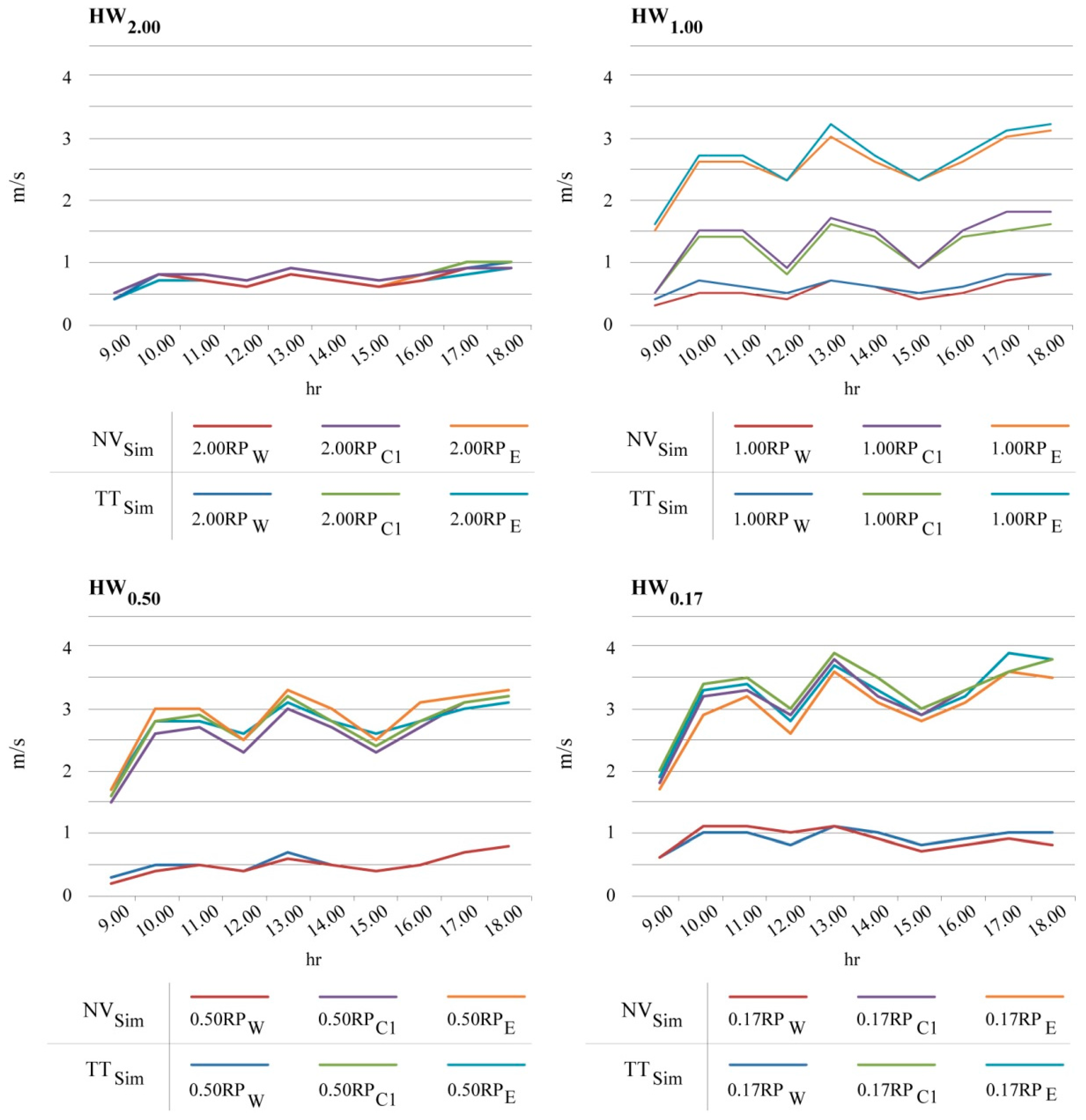
Based upon the calibration of a three-dimensional diagnostic wind model integrated within the program, the last of the eight-tree line was selected to permit the identification of the influence of preceding trees in UCCs (Figure 3). As a result, it was possible to determine how such obstacles within each canyon would influence V_1.1 once it reached each of the designated RPs. Configured within the diagnostic tool within SkyHelios (

Table 6. Specific configurations of SkyHelios wind diagnostic tool.

Calculation Variables	Input	Details
‘Instrument Height’	10 m	Accounting for the meteorological station at a height of 10m
‘Vertical Output Height’	1.1 m	Accounting for gravity centre of the human body which was identical to the stipulated SVF ‘Camera height’ (i.e., target analysis height) of 1.1 m
‘Vertical Displacement Height’	6.6 m	Accounting for the configured structure of the 2.00,1.00,0.50,0.17 UCCs
‘Resolution Output’	1.0 m	To provide sufficiently detailed outputs based upon pretended results, especially for vegetation simulations
‘Wind Direction’	340°	Accounting for the predominant wind patterns predominantly between North and Northwest within the historical quarter of the city [1,54]
Vegetation offset in simulated canyons	50 m	Accounting for possible interference of the wind vortices at the entrance/exit of the examined canyons

), the initial V_1.1 values obtained through Equation (1) could be recalibrated.

3. Results

3.1. General Bioclimatic Conditions during Summer/Winter Periods

3.1.1. Disparities between July and December Bioclimatic Conditions

Demonstrated in Figure 4, the processed microclimatic parameters of T_amb, RH, V_1.1, and Okt obtained from the meteorological station were translated into PS levels for both July and December. As expected, between these two months, there was a large variation of diurnal thermal stress.

During July 2016, PS grades predominantly varied between ‘slight heat stress’ and ‘extreme Heat stress’. In addition, and due to the thermo-physiological indices reaching values which considerably surpassed that of 41 °C, an ‘extreme’ PS grade was added (‘extreme heat stress 2’) to the CTIS calibration to effectively present results which reached 46 °C. Consequently, such an adjustment also relays back to the possibility for expanding the existing ranges of PS upon human beings as presented in Table 2. Such PS stress levels were obtained during days with particularly elevated T_amb values. More precisely, the occurrence of ‘extreme heat stress 2’ took place under two extreme heat events: (1) during a sequential set of days where maximum diurnal T_amb values surpass that of 32 °C—described as an ‘urban heat wave’ by Calheiros [34]; and (2) during a specific day where maximum diurnal T_amb values surpass that of 35 °C—described as a ‘very hot day’ by Miranda [33]. As revealed in Figure 4, July 2016 witnessed three urban heat waves and very hot days, whereby most extreme events were interlinked with one another, with the exception of the 3rd of July. During this specific day, recorded T_amb values almost constantly remained at 35 °C with low V_1.1 values ranging between 1.0 m/s and 2.0 m/s between 12:00 and 16:00 (Table 1).

When considering the results for December 2016, it was evident that the PS thresholds varied differently than those observed for the summer period. More concretely, although only heat stress was observed during July, December revealed both types of thermal stress, particularly during the first half of the month. Such results imply that, whilst Mediterranean climates do witness rare occasions of considerable cold stress (as exemplified during the mornings of the 23rd and 27th), the majority of PS tends to vary between ‘moderate cold stress’ and ‘no thermal stress’. Nonetheless, it was also noted that, particularly between the hours of 12:00 and 15:00, there were also periods surpassing ‘slight heat stress’, as exemplified by the 6th and 10th–12th of December. These outcomes indicate that Lisbon’s thermo-physiological conditions during the winter fluctuate considerably less from thermal comfortable conditions than those obtained during the summer. Regardless it was noted the occurrence of days where, even between 12:00 and 15:00, PS grades still presented ‘Moderate Cold Stress’ as was the case during the 16th of December. Such conditions took place due to a combination of microclimatic characteristics, such as lower diurnal T_amb values (i.e., oscillating between 8.9 °C and 12.4 °C), and higher V_1.1 values (i.e., oscillating between 2.0 m/s and 4.1 m/s) (Table 1).

3.1.2. Comparisons between PET and mPET Indices

The inclusion of both thermo-physiological indices permitted (i) the comparison of PET results against those obtained by a newly adapted mPET index; and (ii) the scrutiny of whether the application of mPET in this study would also collaborate with the general the results obtained by Chen and Matzarakis [31] for western European climates. When cross-examining the outcomes of the two indices for July and December in Figure 4, two major distinctions were acknowledged.

Firstly, in the case of July, it was possible to verify that mPET values very rarely reached a PS of ‘extreme heat stress’. In the sporadic case when mPET did reach such a PS threshold (such as 15:00 during the 3rd of July), it was associated to an extreme heat event (a very hot day). Yet, even under such conditions, and unlike the results obtained by the PET index, the adapted index was distant from ‘extreme heat stress 2’. Concordant with these results, and as discussed within the original study, “almost no extreme hot events were given by the estimation of mPET and only moderate heat stress occurred […] on the contrary, PET [led to] the occurrence of extreme heat stress in Freiburg during the summer” ([31], p. 7).

Secondly, and focusing upon the month of December, it was demonstrated that overall PS values were closer to the PS grade of ‘no thermal stress’ with the use of the mPET index, as opposed to the PS levels obtained by the PET index. Again, such outcomes were also obtained within the original study in Freiburg. Similar to the divergence between the indices for the 3rd of July, colder days such as the 16th of December revealed also lower stress levels through the estimations obtained by mPET.

For these reasons, and based upon the more accurate analysis of the human bio-heat transfer system when exposed to thermal stimuli, the mPET index was used throughout the rest of the study. Such a decision by far devalued the use of the PET index in such studies; rather, it proposed settings in which the preceding index may be complemented b: (i) new improvements to the original Munich energy balance model for individuals model parameters; and (ii) an adjustment of the existing ranges of PS upon human beings.

3.1.3. Day Selection for simulations

Based upon the outputs obtained for both July and December 2016, it was possible to identify the days in which to undertake the simulations within the SkyHelios model. Beyond providing the daily input variables for the particular days, this approach also enabled specific Summer/Winter sun paths to be calibrated into the model. As the intention was to examine the influence of the Tipuana tipu species during annual extreme conditions during the different times of year, both the hottest and coldest days were selected for the simulation of the UCCs. Based upon the identification of the monthly variations of diurnal PS, the 3rd of July and the 16th of December were chosen to represent extreme summer and winter conditions, respectively.

3.2. Canyon RP Outcomes

As identified by existing studies, thermal comfort within urban contexts is strongly affected by urban configurations, whereby morphological elements such as width, height and orientation of a specific canyon are imperative to evaluate precise microclimatic conditions [25,30,82,83,84,85]. Additionally, and through SVF assessments, the impact of vegetation has also been identified as exemplified by Charalampopoulos, Tsiros [86], who determined that, particularly with low SVF values, the presence of vegetation presented positive influences upon thermal comfort conditions. Analogous results obtained by Shashua-Bar, Potchter [17] also indicated such an intrinsic relationship between the thermal effect of trees, with that of urban street geometry.

Undertaking a similar approach to the aforementioned studies, and processed by the SkyHelios model, Figure 5 and Figure 6 present the obtained SVF values for the UCCs. Moreover, based upon the stipulation of the summer paths, it was possible to ascertain the amount of time that each RP was exposed to the sun between 09:00 and 18:00. Such variables were expressed as M_Sum and M_Win to portray the number of minutes each RP was cast in the sun, during the summer and winter, respectively. As expected, M_Sum at each RP was higher given the absence of vegetation. M_Win did not follow this tendency due to its lower winter sun path with the exception for 0.17 RP_N which revealed a reduction in M_Win of 270.

Between the two UCCs orientations, WEO generally resulted in higher durations of solar exposure. Yet, such durations varied between the RPs within the specific canyons. As exemplified by the WEO, considerable differences in M_Sum were identified, as exemplified by 2.00 RP_S obtaining the M_Sum of 130, when 2.00 RP_C2 and 2.00 RP_N revealed higher M_Sum values of 500 and 480, respectively. In the case of HW_0.50, which was the only UCCs in which the central RPs were not placed directly beneath a tree crown, 0.50 RP_C1 and 0.50 RP_C2 still revealed considerable reductions in M_Sum, particularly 0.50 RP_C1. Nevertheless, the highest reductions of M_Sum were obtained in HW_0.17, within all RPs, with a maximum reduction witnessed at 0.17 RP_C1 where M_Sum was reduced by 470.

3.3. Canyon mPET Outcomes

Within this section, the results obtained from SkyHelios and subsequently processed by RayMan to obtain mPET values, and respective PS grades, were demonstrated for each of the four UCCs (Figure 7/Figure 8). In order to facilitate the comprehension of the results, the CTIS program was used to present the (i) differences obtained between the simulations with no vegetation (NV_Sim), against simulations with the presence of the Tipuana tipu species (TT_Sim); and, (ii) identified disparities from the results as initially obtained from the meteorological station. As anticipated, the UCCs with the least amount of thermal stress were HW_2.00 and HW_1.00 which generally presented both lower periods and quantities of thermo-physiological stress. Such was predominantly recognised within the NV_Sim. More precisely, and with regards to the HW_2.00 canyon, it was established that during the:

• 3rd of July within the NSO, the presence of the tree crowns was able to reduce PS levels between 12:00–14:00 by one whole stress grade with a maximum mPET reduction of 6.8 °C (obtained at 14:00 in RPE). Such a decrease represented the capacity of the tree crown to decrease the vulnerability at pedestrian height during the few hours in which the canyon became exposed to direct solar radiation;
• 3rd of July within the WEO, the TT_Sim presented much more prolonged reductions of PS thresholds, especially in RP_N and RP_C2 which were cast in the shade of the vegetative crown between 10:00–15:00 and 10:00–16:00, respectively. During these hours, and in the case of RP_C2, the reduced mPET values ranged between 29.1 °C–37.7 °C, instead of 34.6 °C–42.9 °C as obtained in the NV_Sim;
• 16th December for both the NSO and WEO, it was possible to identify that the absence/presence of vegetation led to no significant differences between the NV_Sim and the TT_Sim. In the case of the NSO, the very subtle variations of PS such as those presented at 12:00 and 16:00 were a result of V_1.1 values oscillating by 0.1 m/s. Within the WEO such distinctions were even less significant, yet as a result of generally higher V_1.1 values (i.e., between 0.2 m/s and 0.7 m/s), all RPs presented slightly colder PS levels.

Within the HW_1.00 canyon, it was determined that during the:

• 3rd of July within the NSO, results were not excessively dissimilar from those obtained in HW_2.00. However, within this UCC, PS levels increased both in stress intensity and duration. Both lateral RPs revealed periods of ‘extreme heat stress’ even in the TT_Sim as exemplified between 12:00–13:00 for RP_W, and at 13:00 for RP_E. Both of these circumstances took place when the sun path crossed the gap between the crown and that of the western/eastern canyon facades. Nevertheless, the diurnal mPET results obtained in the NV_Sim presented much higher PS grades when the canyon was directly exposed to radiation fluxes. Also obtained at RP_E, a maximum reduction in mPET of 7.7 °C was identified when the PS in the NV_Sim almost reached ‘extreme heat stress 2’;
• 3rd of July within the WEO, the results obtained in RP_N show the influence that the vegetative shade could present within the RP until 15:00. At this specific time, both mPET values for the NV_Sim and TT_Sim reached 43.6 °C and 44.1 °C, respectively, thus leading to equally extreme PS grades, which gradually subsided by 18:00;
• 16th December for both the NSO and WEO, and similar to the HW_2.00 canyon, there were very limited variations of thermal conditions between the NV_Sim and TT_Sim. Nevertheless, it was noted that the WEO presented much more stable PS grades between in RP_N/C2/S in comparison to those within the NSO. The justification for this was attributed to the considerable variations of V_1.1 conditions in the entire canyon which were later presented in Figure 9.

When considering the results for the HW_0.50 and HW_0.17, it was verified that overall PS levels increased, and the TT_Sim presented even stronger attenuation results during the summer. Within the HW_0.50 canyon, during the

• 3rd of July within the NSO, due to the increased width of the canyon, the susceptibility to solar radiation was augmented in both the NV_Sim and the TT_Sim. Within the NV_Sim, elevated PS levels increased in duration in comparison to HW_1.00, especially during the morning in RP_W, and the afternoon in RP_C1. Given the placement of the RP_C1 between the edges of two tree crowns within the TT_Sim, it witnessed similar PS grades between 12:00–14:00 to those obtained in the NV_Sim;
• 3rd of July within the WEO, RP_N and RP_C2 presented similar occurrences within the TT_Sim. Whilst cast in the shade within the middle of the canyon, mPET values decreased by up to 6.3 °C as illustrated at 13:00 in RP_C2. When not cast in the shade, however, even the TT_Sim presented PS thresholds reaching ‘extreme heat stress 2’ with mPET values reaching 45.2 °C. Such a value actually exceeded slightly the mPET value of 44.9 °C obtained in NV_Sim as a result of a slightly higher V_1.1 value (+0.2 m/s);
• 16th December for both the NSO and WEO, there still were no clear variations between PS grades between the NV_Sim and the TT_Sim. It was however noted that, between all RPs, the PS grades within RP_C1 and RP_E revealed higher cold stress as a result of higher diurnal V_1.1 values within these two locations (Figure 9).

Lastly, and within the HW_0.17 canyon, it was determined that during the:

• 3rd of July, PS values often reached ‘Extreme Heat Stress 2’ within the NV_Sim. In contrast, within all locations, the highest PS obtained by the TT_Sim was just below the ‘extreme heat stress’ grade as revealed at 17:00 in RP_C1 with a mPET value of 39.6 °C. When comparing the general mPET results between the NV_Sim and the TT_Sim, it was identified that the largest variation between PS thresholds took between 16:00–17:00. As summarised in

  Table 7. Maximum reductions (K) in thermo-physiological indices between simulations with no vegetation (NV_Sim) vs. with the Tipuana tipu (TT_Sim) at each specific location within HW_0.17.

  0.17 RP#	Hour	NVSim		TTSim		K
  		PET °C	mPET °C	PET °C	mPET °C	PET °C	mPET °C
  N	16:00	52.3	46.3	36.7	34.7	−15.6	−11.6
  C2	16:00	47.9	43.5	35.7	34.1	−12.2	−9.4
  S	17:00	48.4	43.5	33.1	31.8	−15.3	−11.6

  , the highest variations took place within the WEO, whereby a maximum reduction of mPET of 11.6 °C (equating to a PET of 15.6 °C) was observed at 16:00 in RP_N;
• 16th of December, the obtained PS levels revealed, for the first time, noteworthy variations between the NV_Sim and the TT_Sim. Such was witnessed particularly within RP_N and RP_C2 between the hours of 12:00 and 15:00, where the TT_SIM presented comparatively colder PS levels as a result of the shade cast by the tree crown. Between the two, RP_N revealed the highest mPET reduction of 2.6 °C (equating to a PET of 2.7 °C) at 12:00. As result, such outcomes suggest the potential of vegetation to induce colder conditions due to obstructing radiation fluxes during the winter.

Analogous to existing studies [1,25,30], the disparity of thermal conditions between those presented from the meteorological station and those obtained from the in-situ assessments were substantial, even in the case of the NV_Sim. Therefore, such outcomes continue to infer the risk of solely considering station values for microscale and studies/projects. On the other hand, these studies also present the methodical means in which to adapt such results into useful data that can be much more valuable for local/microscale thermal sensitive urban design and planning.

Regardless of the considerable differences, there were however associations between the results obtained from the station and those from the ‘in-situ’ assessments. For example, within most of the UCCs it was possible to identify the influence of the accentuated climatic circumstances as initially identified by the station, namely: (i) the elevated T_amb (35.9 °C) and simultaneously low V₁₀ (2.0 m/s) obtained at 15:00 during the 3rd of July 2016; and also, (ii) the low T_amb (9.8 °C) and simultaneously high V₁₀ (8.0 m/s) obtained at 13:00 during the 16th of December 2016.

3.3.1. Wind Influences

As expected, the lower the UCC, the higher the variation of V_1.1 between the different RPs within the canyons. Such variations are presented in Figure 9, which summarises the NSO canyon results obtained through the use of the three-dimensional tool integrated within SkyHelios during the winter period. When considering the modifications of mPET/PS during December, it was possible to make direct associations between the thermal comfort conditions and the V_1.1 results.

When considering the NSO canyons in December, the variations of PS between the RPs (shown in Figure 7 and Figure 8) can be directly linked to the variations of V_1.1 shown in Figure 9. More specifically, to the: (1) HW_2.00 canyon presenting almost identical values at each RP; (2) HW_1.00 canyon revealing the highest values in RP_E, in-between values in RP_C1, and the lowest in RP_W; (3) HW_0.50 revealing equally higher values in RP_E and RP_C2, with lowest values in RP_W; and lastly, (4) HW_0.17 again revealing greater values in RP_E and RP_C2, and RP_W once again revealing the lowest values amongst the three. Thus, it was possible to identify why almost all RP_W PS levels were slightly closer to ‘comfortable conditions’ in comparison to the other two locations in the canyon.

Finally, when considering the vacillation of V_1.1 values between the NV_Sim and the TT_Sim, it was identified that the estimated effects upon wind currents at pedestrian height were fairly inconsequential. Such a result can be attributed to the output of the wind simulations being set at a height of 1.1 m, which fell well beneath the calibrated trunk height (l) of 3 m. Nevertheless, such a result calls for a future study into the effects of vegetation when they are configured closer to one another (i.e., in a cluster) rather than spaced at a considerable distance as calibrated in the TT_Sim. Such a study would also certainly render very different results upon the radiation fluxes at pedestrian height as well.

3.3.2. Tmrt Influences

Contrasting the V_1.1 results, the NV_Sim and the TT_Sim demonstrated very clear deviations of T_mrt in all canyons. As a result of the tree crowns, the casted shade within the RPs led to considerable reductions of radiation fluxes at the pedestrian level.

More specifically, Figure 10 exemplifies such variations of T_mrt within the northern area of the different WEO canyons, whereby (i) even in the case of HW_2.00 (with a canyon width of only 10 m) the crown of the Tipuana tipu was able to reduce T_mrt by 15.6 °C; (ii) in both HW_1.00 and HW_0.50 which presented a similar SVF value, similar T_mrt reductions were of 13.1 °C and 13.3 °C, respectively; and lastly, (iii) the largest difference between the four locations was HW_0.17 which presented a dramatic T_mrt decrease of 29.5 °C. Subsequently, and when referring to the obtained mPET differences between the NV_Sim and the TT_Sim, it was possible to identify the strong correlation with these T_mrt results in each specific RP.

When observing the T_mrt deviations during the winter between the two simulations, smaller, yet important differences were also acknowledged. As shown in Figure 11, due to the Tipuana tipu species maintaining its foliation during the winter, the vegetative crown also reduced radiation fluxes at pedestrian level during December. As a result, in some circumstances (particularly in lower UCCs) this led to the TT_Sim presenting lower comfort conditions. Within the HW_0.17 canyon, and principally in RP_N and RP_C2, it was possible to verify direct results at 13:00 upon the obtained PS grades, even with small reductions of 5.5 °C and 4.6 °C, respectively.

4. Discussion

When considering the results obtained by this study, it became clear that the use of the updated SkyHelios version provided an effective tool to (i) downscale results obtained from Lisbon’s meteorological station and render more accurate outputs for the microclimatic examinations as exemplified by this investigation; and (ii) estimate the in-sit’ effects of the Tipuana tipu species by considering a multitude of climatic variables. Such an examination was complemented with the use of onsite measurements of G_rad in order to attribute more precision to the results obtained by the simulations within each UCC.

Naturally, the results obtained from the model should be approached as estimations of what would take place within actual conditions, particularly with regards to the V_1.1 presented by the new integrated wind analysis tool. As a result, this raises the opportunity to undertake further field studies to further elaborate the results presented by this article. Nevertheless, it was noted that the output speeds during July within the lower UCCs were very similar to those obtained by the field measurements obtained by Nouri and Costa [54] during the summer of 2015 in Lisbon’s historical quarter. In addition, the variation of different speeds within the different regions of the canyon were also analogous, whereby (i) the western regions of the NSO canyon also revealed the lowest wind speeds; and (ii) the central and eastern regions respectively revealed the highest values. Furthermore, and when considering the relationship of all outputs from the NV_Sim and the TT_Sim, it was possible to see clear associations between the different microclimatic variables, namely between the (i) quantity of M_Sum/M_Win values associated to each RP, and the general diurnal thermal conditions within that location; (ii) variations of thermal conditions suggested by the meteorological station, and those obtained within each assessed canyon/location; and, (iii) the impact of climatic variables such as T_amb and V_10/1.1 upon the overall thermo-physiological projections.

The application of the new mPET index within this study also provided the opportunity to both compare and apply a newer PET version based upon an improved thermoregulation model. The results obtained in this study were concomitant with those revealed by Chen and Matzarakis [31], whereby the initial identification of bioclimatic conditions (PET and mPET variables) during the month of July and December did not reveal PS values exceeding that of ‘Extreme Heat Stress’. Although later in the study the mPET results did in fact lead to higher PS grades within the NV_Sim and the TT_Sim, such exacerbations were attributed to the identification of dramatic ‘in-situ’ microclimatic occurrences such as when G_rad values exceeded that of 900 W/m², and other climatic variables such as T_amb were particularly high (such as at 15:00 during the 3rd of July). Such extreme heat conditions, as a result, point to the need to improve the prediction and prevention of such events particularly for the context of Western Europe [87,88].

Within this study, numerous opportunities for future study were identified, namely (1) how mPET/PET entirely based upon variables obtained from the field surveys could differ and/or complement those obtained in this study, especially V values as identified in Nouri and Costa [54]; (2) the opportunity to consider how a group/cluster of trees would present different results, including possible oscillations of V between the NV_Sim and the TT_Sim [76]; (3) the expansion and of PS thresholds to situate mPET/PET results beyond existing levels (e.g., that of 41 °C) as discussed in Nouri, Lopes [10]; (3) following from the previous point, to moreover investigate how mPET outputs may need a general recalibration of existing PS boundaries as already indicated by Chen and Matzarakis [31]; and, lastly (iii) consider how other types of public space design measures, such as misting systems, can be incorporated within vegetative crowns to further augment thermal comfort through the effects of evaporative cooling [89,90].

As stipulated, the 3rd of July and the 16th of December were selected due to their particularly high estimated diurnal stress levels in order to evaluate the potential ‘in-situ’ attenuation effects from the Tipuana tipu. Both days revealed important results, whereby: (i) the summer simulation revealed considerable reductions of PET/mPET of up to 15.6 °C/11.6 °C during a very hot day where diurnal T_amb surpassed that of 35 °C; and, (ii) the winter simulations revealed the risk of over shading within certain conditions, which in turn, led to a reduction of PET/mPET of up to 2.7 °C/2.6 °C. Such results relate directly to the significance of considering year-round implications of shading patterns within outdoor spaces, especially due to their identified dynamic and occasionally dramatic effect upon comfort conditions year round.

5. Concluding Remarks

• Today, in most cases, the urban fabric is already consolidated. As a result, the interdisciplinary practices of urban design and climatology must frequently seek resolutions to address thermal comfort factors in existing UCCs. Consequently, this results in the need for these two disciplines to symbiotically collaborate with one another. This originates the need for practices such public space design to (i) identify existing thermal risk factors; and just as importantly, (ii) produce creative solutions to generate better thermal environments for pedestrians in an era moreover prone to climate aggravations. The types of solutions are numerous, yet this study has focussed upon the use of urban vegetation to obtain such outcomes.
• The study has sought to evaluate how an updated simulation tool and a newly updated thermo-physiological index can contribute to existing studies which recognise the importance of evaluating the in-situ influences of urban vegetation within different urban morphological compositions.
• Focused upon the case of Lisbon, the study identified the in-situ influences of one of the most common shading trees in UCCs which are commonly found within the city’s historical district; one which is known to particularly suffer from high T_amb values and UHI effects during the summer. Notwithstanding, the study also examined the possible negative ‘in-situ’ thermo-physiological impacts that the Tipuana tipu species can have during the winter due to the permanency of its foliage during the colder periods of the year. As a result, the presence of vegetation in different UCCs was approached as an urban element which can both improve and decrease pedestrian thermal comfort during different periods of the year.
• Beyond presenting bioclimatic results (which deliberates upon both singular climatic variables and thermo-physiological stress thresholds), the study suggests the importance of facilitating the transversal comprehension of the outcomes for non-climatic experts to easily interpret such outcomes discussed in the study. As an example, through the use of the CTIS software, the data from the meteorological station and the attained G_rad were translated into easily interpretable figures which are constructed upon the common measuring unit of °C. Even when considering elements such as urban tourism (which is particularly elevated within Lisbon’s historical centre during the summer), such a facilitation can also prove important when safeguarding other urban socio-economic aspects which are also intrinsically dependent upon a thermally comfortable public realm.

References

1. Alcoforado, M.-J.; Andrade, H.; Lopes, A.; Vasconcelos, J. Application of climatic guidelines to urban planning — The example of Lisbon (Portugal). Landsc. Urban Plan. 2009, 90, 56–65. [Google Scholar] [CrossRef]
2. Andrade, H. Bioclima humano e Temperatura do ar em Lisboa. Ph.D. Thesis, Universidade de Lisboa, Lisbon, Portugal, 2003. [Google Scholar]
3. Oliveira, S.; Andrade, H. An initial assessment of the bioclimatic comfort in an outdoor public space in Lisbon. Int. J. Biometeorol. 2007, 52, 69–84. [Google Scholar] [CrossRef] [PubMed]
4. Lopes, A.; Alves, E.; Alcoforado, M.J.; Machete, R. Lisbon urban heat island updated: New highlights about the relationships between thermal patterns and wind regimes. Adv. Meteorol. 2013. [Google Scholar] [CrossRef]
5. Alcoforado, M.J.; Lopes, A.; Lima Alves, E.D.; Canário, P. Lisbon heat island statistical study. Finisterra 2014, 98, 61–80. [Google Scholar]
6. Alcoforado, M.J.; Lopes, A.; Andrade, H.; Vasconcelos, J. Orientações Climáticas Para O Ordenamento Em Lisboa (Relatório 4); Centro de Estudos Geográficos da Universidade de Lisboa: Lisboa, Portugal, 2015. [Google Scholar]
7. Alcoforado, M.J.; Matzarakis, A. Planning with urban climate in different climatic zones. Geographicalia 2010, 57, 5–39. [Google Scholar] [CrossRef]
8. Costa, J.P. Urbanism and Adaptation to Climate Change—The Waterfronts; Livros Horizonte: Lisbon, Portugal, 2013; p. 183. [Google Scholar]
9. Matos-Silva, M.; Costa, J.P. Urban flood adaptation through public space retrofits: The case of Lisbon (Portugal). Sustainability 2017, 9, 816. [Google Scholar] [CrossRef]
10. Nouri, A.S.; Lopes, A.; Costa, J.P.; Matzarakis, A. Confronting potential future augmentations of the physiologically equivalent temperature through public space design: The case of Rossio, Lisbon. Sustain. Cities Soc. 2018, 37, 7–25. [Google Scholar] [CrossRef]
11. Givoni, B. Impact of planted areas on urban environmental quality: A review. Atmos. Environ. 1991, 25, 289–299. [Google Scholar] [CrossRef]
12. Bowler, D.E.; Buyung-Ali, L.; Knight, T.M.; Pullin, A.S. Urban greening to cool towns and cities: A systematic review of the empirical evidence. Landsc. Urban Plan. 2010, 97, 147–155. [Google Scholar] [CrossRef]
13. Qiu, G.-Y.; Li, H.-Y.; Zhang, Q.-T.; Chen, W.; Liang, X.-J.; Li, X.-Z. Effects of evapotranspiration on mitigation of urban temperature by vegetation and urban agriculture. J. Integr. Agric. 2013, 12, 1307–1315. [Google Scholar] [CrossRef]
14. Santamouris, M; Ding, L.; Fiorito, F.; Oldfield, P.; Osmond, P.; Paolini, R.; Prasad, D.; Synnefa, A. Passive and active cooling for the built environment—Analysis and assessment of the cooling potential of mitigation technologies using performance data form 220 large scale projects. Sol. Energy 2016, 154, 14–33. [Google Scholar] [CrossRef]
15. Brown, R.; Gillespie, T. Estimating radiation received by a person under different species of shade trees. J. Aboric. 1990, 16, 158–161. [Google Scholar]
16. Bartholomei, C.; Labaki, L. How much does the change of species of trees affect their solar radiation attenuation? In Proceedings of the fifth international conference on urban climate, Lodtz, Poland, 1–5 September 2003. [Google Scholar]
17. Shashua-Bar, L.; Potchter, O.; Bitan, A.; Boltansky, D.; Yaakov, Y. Microclimate modelling of street tree species effects within the varied urban morphology in the Mediterranean city of Tel Aviv, Israel. Int. J. Climatol. 2010, 30, 44–57. [Google Scholar] [CrossRef]
18. Correa, E.; Ruiz, M.A.; Canton, A.; Lesino, G. Thermal comfort in forested urban canyons of low building density. An assessment for the city of Medonza, Argentina. Build. Environ. 2012, 58, 219–230. [Google Scholar] [CrossRef]
19. De Abreu-Harbich, L.V.; Labaki, L.; Matzarakis, A. Effect of tree planting design and tree species on human thermal comfort in the tropics. Landsc. Urban Plan. 2015, 138, 99–109. [Google Scholar] [CrossRef]
20. Morakinyo, T.E.; Kong, L.; Lau, K.K.L.; Yuan, C.; Ng, E. A study on the impact of shadow-cast and tree species on in-canyon and neighborhood’s thermal comfort. Build. Environ. 2017, 115, 1–17. [Google Scholar] [CrossRef]
21. Ali-Toudert, F.; Mayer, H. Effects of asymmetry, galleries, overhanging façades and vegetation on thermal comfort in urban street canyons. Sol. Energy 2007, 81, 742–754. [Google Scholar] [CrossRef]
22. Ketterer, C.; Matzarakis, A. Human-biometeorlogical assessment of heat stress reduction by replanning measures in Stuttgart, Germany. Landsc. Urban Plan. 2014, 122, 78–88. [Google Scholar] [CrossRef]
23. Qaid, A.; Ossen, D. Effect of asymmetrical street aspect ratios on microclimates in hot, humid regions. Int. J. Biometeorol. 2015, 59, 1–21. [Google Scholar] [CrossRef] [PubMed]
24. Morakinyo, T.E.; Lam, F. Simulation study on the thermal of tree-configuration, planting pattern and wind condition on street-canyon’s micro-climate and thermal comfort. Build. Environ. 2016, 103, 262–275. [Google Scholar] [CrossRef]
25. Algeciras, J.A.R.; Consuegra, L.G.; Matzarakis, A. Spatial-temporal study on the effect of urban street configurations on human thermal comfort in the world heritage city of Camagüey-Cuba. Build. Environ. 2016, 101, 85–101. [Google Scholar] [CrossRef]
26. Algeciras, J.A.R.; Tablada, A.; Matzarakis, A. Effect of asymmetrical street canyons on pedestrian thermal comfort in warm-humid climate of Cuba. Theor. Appl. Climatol. 2017. [Google Scholar] [CrossRef]
27. Nouri, A.S.; Costa, J.P.; Matzarakis, A. Examining default urban-aspect-ratios and sky-view-factors to identify priorities for thermal-sesnsitive public space design in hot-summer Mediterranean climates: The Lisbon case. Build. Environ. 2017, 126, 442–456. [Google Scholar] [CrossRef]
28. Kong, L.; Lau, K.K.L.; Yuan, C.; Chen, Y.; Xu, Y.; Ren, C.; Ng, E. Regulation of outdoor thermal comfort by trees in Hong Kong. Sustain. Cities Soc. 2017, 31, 12–25. [Google Scholar] [CrossRef]
29. Matzarakis, A.; Matuschek, O. Sky view factor as a parameter in applied climatology rapid estimation by the SkyHelios model. Meteorol. Z. 2011, 20, 39–45. [Google Scholar] [CrossRef]
30. Fröhlich, D. Development of a microscale model for the thermal environment in complex areas. Ph.D. Thesis, Fakultät für Umwelt und Natürliche Ressourcen der Albert-Ludwigs-Universität Freiburg, Breisgau, Germany, 2017. [Google Scholar]
31. Chen, Y.-C.; Matzarakis, A. Modified physiologically equivalent temperature — Basics and applications for western European climate. Theor. Appl. Climatol. 2017, 1–15. [Google Scholar] [CrossRef]
32. Peel, M.; Finlayson, B.; McMahon, T. Updated world map of the Koppen-Geiger climate classification. Hydrol. Earth Syst. Sci. 2007, 11, 1633–1644. [Google Scholar] [CrossRef]
33. Miranda, P. The Climate in Portugal during the XX and XXI centuries. In Climate Change in Portugal: Scenarios, Impacts and Adaptation Measures (SIAM); Santos, F., Miranda, P., Eds.; Gradiva: Lisbon, Portugal, 2006; pp. 46–113. [Google Scholar]
34. Calheiros, J. Human Health and Turism Implications. In Climate Change in Portugal: Scenarios, Impacts and Adaptation Measures (SIAM); Santos, F.D., Miranda, P., Eds.; Gradiva: Lisbon, Portugal, 2006; pp. 233–270. [Google Scholar]
35. Lopes, A. Modificações no Clima da Lisboa Como Consequência do Crescimento Urbano. Ph.D. Thesis, University of Lisbon, Lisbon, Portugal, 2003; p. 354. [Google Scholar]
36. Matzarakis, A.; Endler, C. Climate change and thermal bioclimate in cities: Impacts and options for adaptation in Freiburg, Germany. Int. J. Biometeorol. 2010, 54, 479–483. [Google Scholar] [CrossRef] [PubMed]
37. Charalampopoulos, I.; Tsiros, I.; Chronopoulou-Sereli, A.; Matzarakis, A. A methodology for the evaluation fo the human-biolcimatic performance of open spaces. Theor. Appl. Climatol. 2016, 128, 811–820. [Google Scholar] [CrossRef]
38. Algeciras, J.A.R.; Matzarakis, A. Quantification of thermal bioclimate for the management of urban design in Mediterranean climate of Barcelona, Spain. Int. J. Biometeorol. 2015, 8, 1261–1270. [Google Scholar]
39. Roshan, G.; Yousefi, R.; Kovács, A.; Matzarakis, A. A comprehensive analysis of physiologically equivalent temperature changes of Iranian selected stations for the last half century. Theor. Appl. Climatol. 2016. [Google Scholar] [CrossRef]
40. Höppe, P. The physiological equivalent temperature—A universal index for the biometeorological assessment of the thermal environment. Int. J. Biometeorol. 1999, 43, 71–75. [Google Scholar] [CrossRef] [PubMed]
41. Mayer, H.; Höppe, P. Thermal comfort of man in different urban environments. Theor. Appl. Climatol. 1987, 38, 43–49. [Google Scholar] [CrossRef]
42. Matzarakis, A.; Mayer, H.; Iziomon, G.M. Applications of a universal thermal index: Physiological equivalent temperature. Int. J. Biometeorol. 1999, 42, 76–84. [Google Scholar] [CrossRef]
43. Matzarakis, A.; Rutz, F. Rayman Pro—Modelling of Mean Radiant Temperature in Urban Structures Calculation of Thermal Indices; Matzarakis, A., Ed.; Meteorological Institute, University of Freiburg: Freiburg, Germany, 2006. [Google Scholar]
44. Matzarakis, A.; Rutz, F.; Mayer, H. Modelling radiation fluxes in simple and complex environments—Application of the RayMan model. Int. J. Biometeorol. 2007, 51, 323–334. [Google Scholar] [CrossRef] [PubMed]
45. Oliveira, S.; Andrade, H.; Vaz, T. The cooling effect of green spaces as a contribution to the mitigation of urban heat: A case study in Lisbon. Build. Environ. 2011, 46, 2186–2194. [Google Scholar] [CrossRef]
46. Kuttler, W. Stadtklima. In Handbuch der Umweltveränderungen und Ökotoxologie, Band 1B: Atmosphäre; Guderian, R., Ed.; Springer: Berlin, Germany, 2000; pp. 420–470. [Google Scholar]
47. Oke, T.R. Boundary Layer Climates; Routledge: London, UK, 1978. [Google Scholar]
48. McPherson, E. Planting Design for Solar Control. In Energy-Conserving Site Design; McPherson, E., Ed.; American Soceity of Landscape Architects: Washington, DC, USA, 1984; pp. 141–164. [Google Scholar]
49. Brown, R.; Gillespie, T. Microclimatic Landscape Design: Creating Thermal Comfort and Energy Efficiency; John Wiley and Sons: New York, NY, USA, 1995. [Google Scholar]
50. Klemm, W.; Heusinkveld, B.G.; Lenzholzer, S.; van Hove, B. Street greenery and its physical and psychological impact on thermal comfort. Landsc. Urban Plan. 2015, 138, 1–12. [Google Scholar] [CrossRef]
51. Streiling, S.; Matzarakis, A. Influence of single and small clusters of trees on the bioclimate of a city: A case study. J. Arboric. 2003, 29, 309–317. [Google Scholar]
52. Erell, E.; Pearlmutter, D.; Williamson, T. Urban Microclimate—Designing the Spaces between Buildings; Earthscan: London, UK, 2011. [Google Scholar]
53. Brown, R.; Vanos, J.; Kenny, N.; Lenzholzer, S. Designing urban parks that ameliorate the effects of climate change. Landsc. Urban Plan. 2015, 138, 1–14. [Google Scholar] [CrossRef]
54. Nouri, A.S.; Costa, J.P. Addressing thermophysiological thresholds and psychological aspects during hot and dry Mediterranean summers through public space design: The case of Rossio. Build. Environ. 2017, 118, 67–90. [Google Scholar] [CrossRef]
55. Brown, R.; Cherkezoff, L. Of what comfort value, a tree? J. Arboric. 1989, 15, 158–162. [Google Scholar]
56. Tsiros, I. Assessment and energy implications of street air temperature cooling by shade trees in Athens (Greece) under extremely hot weather conditions. Renew. Energy 2010, 35, 1866–1869. [Google Scholar] [CrossRef]
57. Röckle, R. Bestimmung der Strömungsverhältnisse im Bereich komplexer Bebauungsstrukturen. Ph.D. Thesis, Techn. Hochschule Darmstadt, Darmstadt, Germany, 1990. [Google Scholar]
58. Bagal, N.; Pardyjak, E.; Brown, M. Improved upwind cavity parameterizations for a fast response urban wind model. In Proceedings of the AMS Symposium on Planning, Nowcasting, and Forecasting in the Urban Zone, Seattle, WA, USA, 11–15 January 2004. [Google Scholar]
59. Singh, B.; Singh, B.; Hansen, B.S.; Brown, M.J.; Pardyjak, E.R. Evaluation of the QUIC-URB fast response urban wind model for a cubical building array and wide building street canyon. Environ. Fluid Mech. 2008, 8, 281–312. [Google Scholar] [CrossRef]
60. Staiger, H.; Laschewski, G.; Gratz, A. The perceived temperature—A versatile index for the assessment of the human thermal environment. Part A: Scientific basics. Int. J. Biometeorol. 2012, 56, 165–176. [Google Scholar] [CrossRef] [PubMed]
61. Jendritzky, G.; de-Dear, R.; Havenith, G. UTCI—Why another thermal index? Int. J. Biometeorol. 2012, 56, 421–428. [Google Scholar] [CrossRef] [PubMed] [Green Version]
62. Matzarakis, A. Transfer of climate data for tourism applications—The Climate-Tourism/Transfer-Information-Scheme. Sustain. Environ. Res. 2014, 24, 273–280. [Google Scholar]
63. Lin, T.-P.; Matzarakis, A. Tourism climate and thermal comfort in Sun Moon Lake, Taiwan. Int. J. Biometeorol. 2008, 52, 281–290. [Google Scholar] [CrossRef] [PubMed]
64. Matzarakis, A.; Rocco, M.D.; Najjar, G. Thermal bioclimate in Strasburg—The 2003 heat wave. Theor. Appl. Climatol. 2009, 98, 209–220. [Google Scholar] [CrossRef]
65. Zaninovic, K.; Matzarakis, A. The bioclimatological leaflet as a means conveying climatological information to tourists and the tourism industry. Int. J. Biometeorol. 2009, 53, 369–374. [Google Scholar] [CrossRef] [PubMed]
66. Matzarakis, A.; Mayer, H. Heat Stress in Greece. Int. J. Biometeorol. 1997, 41, 34–39. [Google Scholar] [CrossRef] [PubMed]
67. Almeida, A.L.B. The Value of Trees: The Trees and Urban Forests of Lisbon. Ph.D. Thesis, Superior Institute of Agronomy, Lisbon, Portugal, 2006; p. 342. [Google Scholar]
68. Soares, A.L.; Rego, F.C.; McPherson, E.G.; Simpson, J.R.; Peper, P.J.; Xiao, Q. Benefits and costs of street tree in Lisbon, Portugal. Urban For. Urban Gree. 2011, 10, 69–78. [Google Scholar] [CrossRef]
69. Saraiva, G.A.N.; de Almeida, A.F. Árvores na Cidade Roteiro das Árvores Classificadas de Lisboa; By The Book: Lisbon, Portugal, 2016. [Google Scholar]
70. Torre, J. Vegetation as an Instrument for Microclimatic Control. Ph.D. Thesis, Universitat Politècnica de Catalunya, Barcelona, Spain, 1999. [Google Scholar]
71. Coello, A.; Philippe, O. Canopia Urbana: Plaça de les Glories Catalanes—Barcelone; Agence TER: Barcelona, Spain, 2015; pp. 1–36. [Google Scholar]
72. De Vilardaga, A.; Vinas, X.N.; Solanich, F.P.; Montllo, J.S. El Árbol en Jardinería y Paisajismo Guía de Aplicación para España y países de Clima Mediterráneo y Templado, 2nd ed.; Ediciones Omega: Barcelona, Spain, 1995. [Google Scholar]
73. Fahmy, M.; Sharples, S. Urban form, thermal comfort and building CO2 emissions—A numerical analysis in Cairo. Build. Serv. Eng. Res. Technol. 2011, 32, 73–84. [Google Scholar] [CrossRef]
74. Berry, R.; Livesley, S.; Aye, L. Tree canopy shade impacts on solar irradiance received by building walls and their surface temperature. Build. Environ. 2013, 69, 91–100. [Google Scholar] [CrossRef]
75. Fahmy, M.; Sharples, S. On the development of an urban passive thermal comfort system in Cairo, Egypt. Build. Environ. 2009, 44, 1907–1916. [Google Scholar] [CrossRef]
76. Abreu-Harbich, L.V.; Labaki, L.; Matzarakis, A. Reduction of mean radiant temperature by cluster of trees in urban and architectural planning in tropical climate. In Proceedings of the PLEA2012–28th Conference: Opportunities, Limits & Needs–Towards an Environmentally Responsible Architecture, Lima, Perú, 7–9 November 2012. [Google Scholar]
77. Olgyay, V. Design with Climate, Bioclimatic Approach to Architectural Regionalism; Princeton University Press: New Jersey, NJ, USA, 1963. [Google Scholar]
78. Whyte, W.H. The Social Life of Small Urban Spaces; Project for Public Spaces Inc.: New York, NY, USA, 1980. [Google Scholar]
79. Norton, B.; Coutts, A.M.; Livesley, S.J.; Harris, R.J.; Hunter, A.M.; Williams, N.S. Planning for cooler cities: A framework to prioritise green infrastructure to mitigate high temperatures in urban landscapes. Landsc. Urban Plan. 2015, 134, 127–138. [Google Scholar] [CrossRef]
80. Shashua-Bar, L.; Tsiros, I.X.; Hoffman, M. Passive cooling design options to ameliorate thermal comfort in urban streets of a Mediterranean climate (Athens) under hot summer conditions. Landsc. Urban Plan. 2012, 57, 110–119. [Google Scholar] [CrossRef]
81. Lin, T.-P.; Tsai, K.T.; Hwang, R.L.; Matzarakis, A. Quantification of the effect of thermal indices and sky view factor on park attendance. Landsc. Urban Plan. 2012, 107, 137–146. [Google Scholar] [CrossRef]
82. Herrmann, J.; Matzarakis, A. Mean radiant temperature in idealised urban canyons—Examples from Freiburg, Germany International. Int. J. Biometeorol. 2012, 56, 199–203. [Google Scholar] [CrossRef] [PubMed]
83. Matzarakis, A.; Fröhlich, D.; Gangwisch, M. Effect of radiation and wind on thermal comfort in urban environments—Applications of the RayMan and SkyHelios model. In Proceedings of the 4th International Conference on Countermeasures to Urban Heat Island, National University of Singapore, Singapore, 30 May–1 June 2016. [Google Scholar]
84. Nouri, A.S.; Costa, J.P. Placemaking and climate change adaptation: New qualitative and quantitative considerations for the “Place Diagram”. J. Urbanism: Int. Res. Placemaking Urban Sustain. 2017, 10, 1–27. [Google Scholar]
85. Charalampopoulos, I. Development of a Methodology and Applications for the Bioclimatic Conditions’ Evaluation of Open Space with Diverse Configurations (In Greek). Ph.D. Thesis, Agricultural University of Athens, Athens, Greece, 2019. [Google Scholar]
86. Charalampopoulos, I.; Tsiros, I.; Chronopoulou-Sereli, A.; Matzarakis, A. Analysis of thermal bioclimate in various urban configurations in Athens, Greece. Urban Ecosyst. 2013, 16, 217–233. [Google Scholar] [CrossRef]
87. Kovats, R.; Ebi, K. Heatwaves and public health in Europe. J. Public Health 2006, 16, 592–599. [Google Scholar] [CrossRef] [PubMed]
88. Matzarakis, A. The Heat Health Warning System of DWD—Concept and Lessons Learned. In Perspectives on Atmospheroc Sciences; Karacostas, T., Bais, A., Nastos, P., Eds.; Springer International Publishing: Gewerbestrasse, Switzerland, 2016; pp. 191–196. [Google Scholar]
89. Alvarez, S.; Rodriguez, E.; Martin, R. Direct Air Cooling from Water Drop Evaporation, in PLEA 91—Passive and Low Energy Architecture; PLEA: Seville, Spain, 1991. [Google Scholar]
90. Ishii, T.; Tsujimoto, M.; Yoon, G.; Okumiya, M. Cooling system with water mist sprayers for mitigation of heat-island. In Proceedings of the Conference Seventh International Conference on Urban Climate, ICUC, Yokohama, Japan, 29 June–3 July 2009. [Google Scholar]
Figure 1. Comparison of monthly averages of Tamb and relative humidity (RH) field recordings obtained without the presence of a shading tree against those obtained directly beneath a vegetative crown in the central area of a low urban canyon case (UCC) in Lisbon’s historical district | Source: Adapted from [54].
Atmosphere 09 00012 g001
Figure 2. Representation of the Tipuana tipu species | (A) Example of linear planation of species within the eastern lateral sidewalk in Rossio during the afternoon | (B) Dimensions of tree of which were later used in simulations | (C) Annual foliation and coloration of vegetative crown—adapted from Viñas, Solanich [72].
Atmosphere 09 00012 g002
Figure 3. North-to-south orientation (NSO) layout of the determined urban canyon cases (UCCs) and the central/lateral reference points (RPs) with specified crown spreads and vegetative coverage ratios (VCR); A-A cross-section in HW2.00, B-B cross-section in HW1.00, C-C cross-section in HW0.50, D-D cross-section in HW0.17
Atmosphere 09 00012 g003
Figure 4. Variations of diurnal physiological stress (PS) based upon physiologically equivalent temperature (PET) and modified PET (mPET) at an hourly interval between 09:00 and 18:00 for July and December 2016 with identification of urban heat waves (UHW) and very hot days (VHD).
Atmosphere 09 00012 g004
Figure 5. Identification of SVF and minutes cast in the sun during the summer/winter (MSum/MWin) between 09:00–18:00 for each RP for HW2.00 and HW1.00.
Atmosphere 09 00012 g005
Figure 6. Identification of SVF and minutes cast in the sun during the summer/winter (MSum/MWin) between 09:00–18:00 for each R for HW0.50 and HW0.17.
Atmosphere 09 00012 g006
Figure 7. Canyon variations of diurnal PS resultant of hourly mPET between canyon simulations with no vegetation (NV) vs. with the Tipuana tipu (TT) and those originally presented by the meteorological station for HW2.00 and HW1.00.
Atmosphere 09 00012 g007
Figure 8. Canyon variations of diurnal PS resultant of hourly mPET between canyon simulations with NV vs. with the Tipuana tipu (TT) and those originally presented by the meteorological station for HW0.50 and HW0.17.
Atmosphere 09 00012 g008
Figure 9. Diurnal wind speed (V1.1) variations between the RPs within all NSO canyons for the 16th of December.
Atmosphere 09 00012 g009
Figure 10. Mean radiant temperature (Tmrt) differences during the summer at selected RPs between simulations with No Vegetation (NVSim) vs. with the Tipuana tipu (TTSim) during the 3rd of July.
Atmosphere 09 00012 g010
Figure 11. Mean radiant temperature (Tmrt) differences during the summer at selected RPs between simulations with no vegetation (NVSim) vs. with the Tipuana tipu (TTSim) during the 16th of December.
Atmosphere 09 00012 g011