Estimating the Biogenic Non-Methane Hydrocarbon Emissions over Greece

Abstract

Biogenic emissions affect the urban air quality as they are ozone and secondary organic aerosol (SOA) precursors and should be taken into account when applying photochemical pollution models. The present study presents an estimation of the magnitude of non-methane volatile organic compounds (BNMVOCs) emitted by vegetation over Greece. The methodology is based on computation developed with the aid of a Geographic Information System (GIS) and theoretical equations in order to produce an emission inventory on a 6 × 6 km² spatial resolution, in a temporal resolution of 1 h covering one year (2016). For this purpose, a variety of input data was used: updated satellite land-use data, land-use specific emission potentials, foliar biomass densities, temperature, and solar radiation data. Hourly, daily, and annual isoprene, monoterpenes, and other volatile organic compounds (OVOCs) were estimated. In the area under study, the annual biogenic emissions were estimated up to 472 kt, consisting of 46.6% isoprene, 28% monoterpenes, and 25.4% OVOCs. Results delineate an annual cycle with increasing values from March to April, while maximum emissions were observed from May to September, followed by a decrease from October to January.

1. Introduction

Volatile organic compounds (VOCs) are emitted into the atmosphere from anthropogenic and natural sources in the marine and terrestrial environment. Vegetation naturally releases VOCs, collectively referred to as biogenic non-methane volatile organic compounds (BNMVOC), with isoprene (C₅H₈) and monoterpenes (C₁₀H₁₆) being the most abundant species. The remaining biogenic emitted species consist of a number of oxygenated compounds, such as alcohols and aldehydes, and they are referred to as other VOCs (OVOCs) [1,2].

Globally, biogenic sources of volatile organic compounds are estimated to exceed those from anthropogenic sources by a factor of ten to one [3]. In Europe, anthropogenic and biogenic NMVOCs emissions have comparable magnitudes: annual BNMVOC emissions are estimated at 14 Tg compared to man-made emissions of around 24 Tg [3,4] estimated up to 5% increase in summer daily ozone maxima over Europe due to BNMVOC emissions, the highest values appearing over the Mediterranean region, dominated by emissions from vegetation during summertime. This region has a complex vegetal biodiversity quite different from the usual northern latitude or US vegetation, as it receives high fluxes of solar radiation in the summertime and is dominated by high temperatures. Finally, high ozone concentrations are often very pronounced due to primary pollutant emissions in a regional scale dominated by high radiation fluxes and temperature values [5].

The calculation of their fluxes is an important input in air quality models, since they are highly reactive in the troposphere by affecting regional photochemical processes [6]. They react with the hydroxyl radical, ozone, and the nitrate radical, resulting in the formation of carbon monoxide and organic species (including secondary organic aerosols) that can enhance concentrations of ozone and other oxidants in environments rich in nitrogen oxides [7]. On a global cycle, biogenic volatile organic compounds (BVOCs) contribute to the global carbon cycle and have a key role in the global climate [1]. Furthermore, most of them are oxidized to carbon dioxide (CO₂) into the atmosphere and determine the growth rate of atmospheric methane concentrations [1].

The BVOCs emissions depend on the different types of vegetation and meteorological conditions. Concerning the isoprene, it has been shown that it is emitted mainly from deciduous trees under high temperature and Photosynthetically Active Radiation (PAR) conditions [1]. On the other hand, monoterpenes are emitted mostly by coniferous trees. They are mainly temperature-dependent, except for some evergreen oaks and Norway spruce that are temperature- and light-dependent [8].

Presently in Greece, there does not exist a detailed gridded database with recent data concerning the biogenic emissions. Earlier efforts by [9] and [2] included the Balkans and Greece on a 10 km resolution or Europe on a 30 km resolution, respectively. They were either in the form of an emissions model or a Geographic Information System (GIS) database, respectively, and were based on the equations introduced [10] for the computation of isoprene, monoterpene, and OVOCs emission fluxes and used as input land use, foliar biomass densities, emission potentials, temperature, and solar radiation. Both studies used old land-use data (1993 and 2010, respectively) and climatic data that originated either from inversely interpolated global mean monthly temperatures or modelled from MM5/TUV (reference year 2003 or older). Moreover, they reported significant differences with other existing works. Few studies have applied the MEGAN model to estimate the BVOC emissions impact on the O₃ and PM levels above Europe and Greece, such as [11]. In fact, the MEGAN model is based on the equations by [10] and uses meteorological input data from MM5/TUV. Finally, it must be mentioned that only few experimental studies of VOCs including isoprene and monoterpenes took place in rural and urban areas of Greece, such as those reported by [12] and [13], indicated clearly the significant contribution of vegetation, more than 60% to the measured isoprene and monoterpene levels, as well as the dependence of isoprene production to sunlight and temperature. The present work aims to present results of the computed BNMVOC emissions over Greece with the aid of a GIS database, the well-known and accepted equations by [10] and, as opposed to the abovementioned works, temperature data obtained from the extended ground-based monitoring network of meteorological stations covering Greece (www.meteo.gr). Moreover, photochemically active radiation was obtained from the SOLEA application. The new BNMVOC inventory covers the year 2016 and has the possibility to be regularly updated to include more years. The paper is organized as follows: in Section 2, the methodology used (the mathematical and computational model) for the estimation of the biogenic emissions is introduced. Section 3 focuses on the results of our study, presenting the spatially resolved isoprene, monoterpenes, and OVOCs biogenic emissions, as well as a short discussion concerning the results. A summary and conclusions are provided in Section 4.

2. Methodology

2.1. The Mathematical Model

In the present study, the mathematical model for estimating isoprene, monoterpenes, and OVOCs emissions in Greece was incorporated into the GIS platform. The mathematical model used for all types of vegetation, describing the emissions flux on an hourly basis is that of [10]:

$$\mathrm{Flux}\left({\mathsf{\mu }\mathrm{g}\mathrm{m}}^{-2}{\mathrm{yr}}^{-1}\right)=\int \mathsf{\epsilon }·\mathrm{D}·\mathsf{\gamma }\mathrm{dt}$$

(1)

where ε is the emission potential (${\mathsf{\mu }\mathrm{g}\mathrm{g}}^{-1}{\mathrm{h}}^{-1}$) for any particular species, D is the foliar biomass density ($\mathrm{g}\mathrm{dry}\mathrm{weight}\mathrm{foliage}{\mathrm{m}}^{-2}$), and γ is a unit less environmental correction factor representing the effects of short-term (e.g., hourly) temperature and solar radiation changes on emissions. We have to underline that the experiments were conducted using eucalyptus trees (Eucalyptus globulus L.).

Concerning the estimation of the isoprene emissions, [14] showed that, to a very good approximation, the short-term (e.g., hourly) variations in emissions could be described by the product of a light-dependent factor and a temperature-dependent factor. So, the environmental correction factor for the isoprene emission is expressed as:

$${\mathsf{\gamma }}_{\mathrm{iso}}={\mathrm{C}}_{\mathrm{L}}·{\mathrm{C}}_{\mathrm{T}}.$$

(2)

The light-dependent factor is given by:

$${\mathrm{C}}_{{\mathrm{L}}_{\mathrm{iso}}}=\frac{{\mathrm{a}\mathrm{C}}_{{\mathrm{L}}_1}\mathrm{L}}{\sqrt{1}+{\mathrm{a}}^2{\mathrm{L}}^2}$$

(3)

where a = 0.0027 and ${\mathrm{C}}_{{\mathrm{L}}_1}=1.066$ are empirical constants, and L is the PAR flux ($\mathsf{\mu }\mathrm{mol}\mathrm{photons}\left(400–700\mathrm{nm}\right) {\mathrm{m}}^{-2}{\mathrm{s}}^{-1})$.

The temperature-dependent factor is given by:

$${\mathrm{C}}_{{\mathrm{T}}_{\mathrm{iso}}}=\frac{\exp (\frac{{\mathrm{C}}_{{\mathrm{T}}_1}\left({\mathrm{T}-\mathrm{T}}_{\mathrm{s}}\right)}{{\mathrm{R}\mathrm{T}}_{\mathrm{s}}\mathrm{T}}}{1+\exp (\frac{{\mathrm{C}}_{{\mathrm{T}}_2}\left({\mathrm{T}-\mathrm{T}}_{\mathrm{M}}\right)}{{\mathrm{R}\mathrm{T}}_{\mathrm{s}}\mathrm{T}}}$$

(4)

where R is the gas constant ($=8.314\mathrm{J}{\mathrm{K}}^{-1}{\mathrm{mol}}^{-1}$), ${\mathrm{C}}_{{\mathrm{T}}_1}\left(=\mathrm{95,000}\mathrm{J}{\mathrm{mol}}^{-1}\right)$, ${\mathrm{C}}_{{\mathrm{T}}_2}=\left(\mathrm{230,000}\mathrm{J}{\mathrm{mol}}^{-1}\right)$, and ${\mathrm{T}}_{\mathrm{M}}\left(=314\mathrm{K}\right)$ are empirical coefficients based upon measurements of three plant species—eucalyptus, aspen, and velvet bean—but which seem to be valid for a variety of different plant species [14], and finally, ${\mathrm{T}}_{\mathrm{s}}\left(=303\mathrm{K}\right)$ is the standard temperature. More precisely, the above equation accounts the influence of temperature on electron transport and is a simplified form of the enzyme activation equations [14]. Initial fits for ${\mathrm{C}}_{{\mathrm{T}}_1}$, ${\mathrm{C}}_{{\mathrm{T}}_2}$, and ${\mathrm{T}}_{\mathrm{M}}$ (at each light intensity level) revealed no significant trend in the values of three constants with light intensity. The values used represent the best fit for all light intensities and temperature.

Concerning the estimation of the monoterpene emissions, the environmental correction factor suitable for most of the plants is parameterized using the following equation [14]:

$${\mathsf{\gamma }}_{\mathrm{mts}}=\exp \left(\mathsf{\beta }\left({\mathrm{T}-\mathrm{T}}_{\mathrm{s}}\right)\right)$$

(5)

where $\mathsf{\beta }(=0.09{\mathrm{K}}^{-1})$ is an empirical coefficient based on non-linear regression analysis of numerous measurements present in the literature.

Recent studies proved that monoterpene emissions from some evergreen oaks and also Norway spruce show a light dependency, which seems to be well described by the isoprene environmental correction factor [8].

Since the environmental conditions controlling emissions of OVOCs are not entirely understood compared to isoprene and monoterpenes, and given the lack of other information, OVOCs emissions are considered temperature-dependent and the use of Equation (5) is recommended for the estimation of their emissions [15].

2.2. The Computational Model

In order to produce the NMVOCs emission inventory for Greece on a 6 × 6 ${\mathrm{km}}^2$ spatial and a 1hr temporal resolution covering one year, the GIS software (ArcView v10) was used in order to combine a variety of input data: updated satellite land-use data, land-use specific emission potentials, foliar biomass densities, temperature, and solar radiation data. For the calculation of the hourly biogenic emissions, detailed meteorological data for the time period of a whole year (2016) were used. After calculating the hourly emission fluxes, daily, monthly, and yearly emission values were also estimated.

The land use–land cover (LULC) data used in the present study was provided by the United States Geological Survey (USGS) Global LULC version 2.0 Database derived from the 1 km Advanced Very High Resolution Radiometer (AVHRR) data. The USGS classification system includes 25 land cover categories, only 14 of which are found in the area under study (Figure 1). The different land-use classes emitting BVOC are characterized by one ecosystem type (e.g., Grassland) or a combination of two of them (e.g., Mixed Scrubland–Grassland). The area was divided into cells using a spatial resolution of 6 × 6 ${\mathrm{km}}^2$ with Lambert Conic Conformal projection. Each cell was checked separately and correction of the LULC category was made if necessary based on the work done by [5,16]. As a result, new updated land-use data were used for the year 2016 that depict the all the changes that took place the recent years in Greece and especially the urban areas.

The employment of land-use specific emission potentials and foliar biomass densities for every month covering the whole year is essential for the estimation of isoprene, monoterpenes, and OVOCs. The main references used for the selection of these values were from the recent study of [17] under the NatAir program (Improving and Applying Methods for the Calculation of Natural and Biogenic Emissions and Assessment of Impacts on Air Quality) for the region of Europe and the neighboring ones. The existing databases were used and updated according to recent experimental findings. Plant species-specific emission factors were updated and recalculated in order to assign foliar biomass densities and emission potentials to commonly observe European vegetation species. Furthermore, the fact that the foliar biomass densities are not constant during the year was taken into account. In order to describe the seasonal variation of the foliar biomass densities, it was necessary to use corrective factors which vary between the different vegetation species according to the study of [9]. So, appropriate monthly foliar biomass densities were assigned to each land-use category. The maximum monthly foliar biomass densities are observed during May, June, July, August, and September while the minimum ones are observed during December, January, and February. Indicatively, in

Table 1. Foliar biomass densities ($\mathrm{g}\mathrm{dry}\mathrm{weight}\mathrm{foliage}{\mathrm{m}}^{-2}$) and emission potentials ($\mathsf{\mu }\mathrm{g}{\mathrm{g}}^{-1}{\mathrm{h}}^{-1}$) for the observed land-use categories in Greece for the months of January and July.

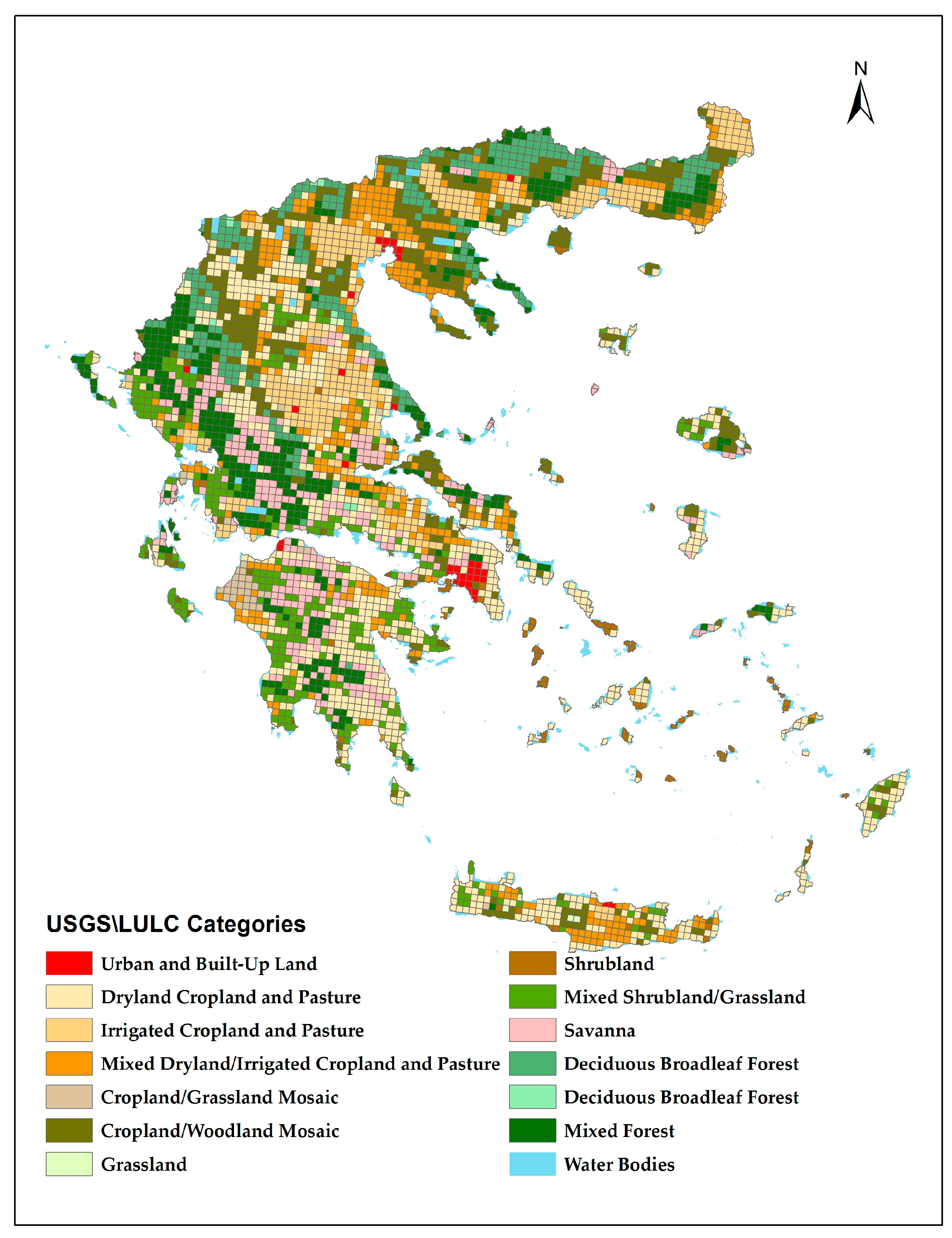
Land-Use Category	January			July
	Foliar Biomass Density	Isoprene Emission Potential	Monoterpene Emission Potential	Foliar Biomass Density	Isoprene Emission Potential	Monoterpene Emission Potential
Urban and Built-Up Land	50	2	1	100	2	1
Dryland Cropland and Pasture	25	0.5	0.5	100	0.5	0.5
Irrigated Cropland and Pasture	300	0.5	0.5	300	0.5	0.5
Mixed Dryland–Irrigated Cropland and Pasture	194	1.1	0.95	325	1.85	1.56
Cropland–Grassland Mosaic	156	0.5	0.5	175	0.5	0.5
Cropland/Woodland Mosaic	200	1.6	1.6	200	1.63	1.63
Grassland	12.5	0.5	0.5	50	0.5	0.5
Shrubland	87.5	3	2.5	350	3	2.5
Mixed Shrubland–Grassland	50	2.69	2.25	200	2.69	2.25
Savanna	56.3	4.5	4.5	75	3.5	3.5
Deciduous Broadleaf Forest	0	30	0.5	340	30	0.5
Evergreen Needleleaf Forest	700	1	2.5	700	1	2.5
Mixed Forest	250	7	3	500	7	3
Water Bodies	0	0	0	0	0	0

, the values of a winter (January) and a summer month (July) are presented. When a land-use class was characterized by a combination of different vegetation species, it was assumed that the monthly average foliar biomass density is equal to the mean value of the foliar biomass densities of all vegetation types within the land-use category [9]. Finally, the specific emission potentials for the land-use classes that are a combination of different vegetation types were calculated using the formula:

$$\mathsf{\epsilon }=\frac{{\displaystyle \sum }(\frac{{\mathsf{\epsilon }}_{\mathrm{i}}{\mathrm{D}}_{\mathrm{i}}}{\mathrm{n}})}{{\displaystyle \sum }(\frac{{\mathrm{D}}_{\mathrm{i}}}{\mathrm{n}})}$$

(6)

where ${\mathsf{\epsilon }}_{\mathrm{i}}$ and ${\mathrm{D}}_{\mathrm{i}}$ are the emission potentials and the foliar biomass densities of each vegetation type within the land-use category, and n is the number of vegetation types within the land-use category [9].

Finally, for the OVOCs, due to lack of reliable experimental data on their emissions, [9] recommended the use of the uniform emission rate of 1.5 $\mathsf{\mu }\mathrm{g}{\mathrm{g}}^{-1}{\mathrm{h}}^{-1}$ for the different vegetation species.

Hourly temperature values were provided by the National Observatory of Athens (www.meteo.gr) from 292 meteorological stations for 2016. The typical temperature diurnal variation for all the stations was produced by calculating the average hourly temperature values of each month of the year. Hourly temperature maps were constructed using the technique of Inverse Distance Interpolation (IDW), thus providing a continuous temperature field covering the area under study.

Solar radiation data have been calculated with the use of an existing methodology [18] that has been used in the pilot study SENSE of the Geo-Crandle project (http://geocrandle.eu/en/). It is based on solar irradiance spectra produced via a synergy of satellite data, radiative transfer simulations, and neural network techniques. The method has been validated in [19] by comparison with ground-based solar radiation measurements. The radiation SENSE output for every month of 2016 having 0.05° latitude by 0.05° longitude spatial resolution and 1 h temporal resolution. Indicatively, in Figure 2, the mean daily PAR for January and July are presented. Then, with the aid of GIS, these radiation values were adjusted to the area of interest with a spatial resolution of 6 × 6 km².

Initially, the hourly biogenic emissions were calculated using the typical temperature and radiation diurnal variation of each month of 2016. Then, the monthly biogenic emissions were estimated by summing up the daily emissions of isoprene, monoterpenes, and OVOCs per month in Greece, and finally, the annual ones were estimated as the sum of the total monthly emissions for 2016 per hydrocarbon.

3. Results

The total biogenic NMVOCs emissions over the study area are estimated to be 473 kt, consisting of 220 kt of isoprene, 132 kt of monoterpenes, and 120 kt of OVOCs. Figure 3 and Figure 4 illustrate the spatial distribution of annual isoprene and monoterpene emissions over Greece. Maximum isoprene emissions are about 545.11 tones per cell. Spatially, these maximum values are observed above mixed forests and deciduous broadleaf forests located in the area of Thrace, West Thessaly, Peloponnese, Epirus (Pindus Mountains), Lesvos, and Macedonia. Concerning the monoterpenes, peak emission values are about 188.7 tones per cell. The land-use categories characterized by high monoterpene emissions are the mixed forests and the mixed dryland–irrigated cropland and pasture and are located to the Western Epirus, Central Greece, Euboea, Lesvos, central Peloponnese, and Thrace. Finally, the maximum OVOCs emission observed to the area of Greece is up to 112.9 tn/cell. This maximum value is the lowest compared to the maximum values of isoprene and monoterpene emissions. The areas characterized by high OVOCs emissions are the same as the monoterpene ones.

As it was expected, the BVOC emissions take their maximum values during summertime, and more precisely, in July. A winter month (January) and a summer month (July) were chosen to be presented in the present study. More precisely, isoprene emissions during summer reach the 148.71 tones per cell, while on the other hand, in January much lower isoprene emissions were estimated as expected (Figure 5). The land-use categories that are characterized by maximum isoprene emissions are the mixed forests and the deciduous broadleaf forests because of their high emission potential and foliar biomass density.

The isoprene emissions during summer are higher than the monoterpene and OVOCs ones, but during winter the monoterpene and OVOCs emissions are higher because of the dependency of isoprene emissions on solar radiation. Indicatively, in July, the isoprene emissions contribute up to 53.6% to the total biogenic emissions, with monoterpenes’ contribution being only up to 24.4% and OVOCs’ up to 22% (

Table 2. Percentage (%) of contribution of each hydrocarbon to the total monthly biogenic emissions.

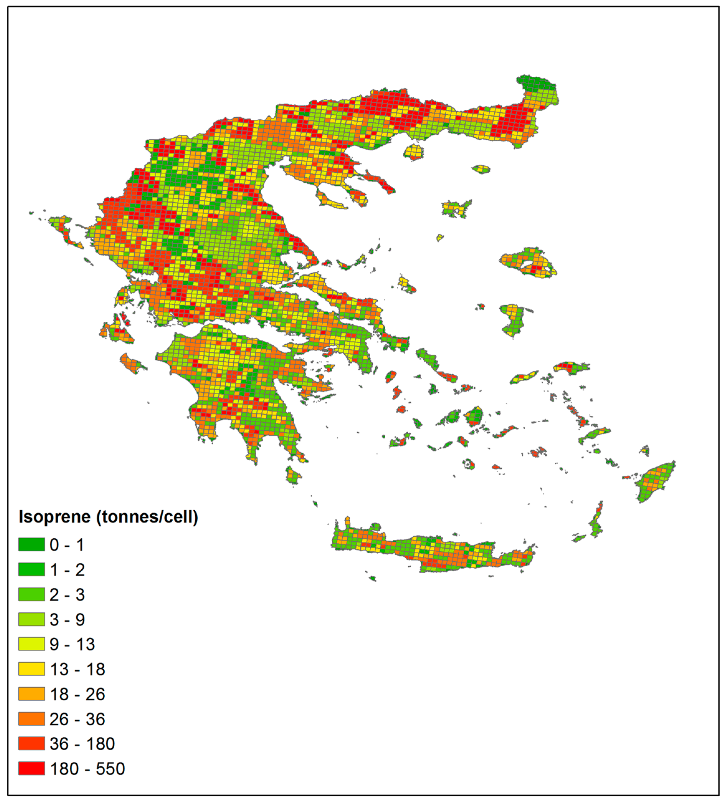
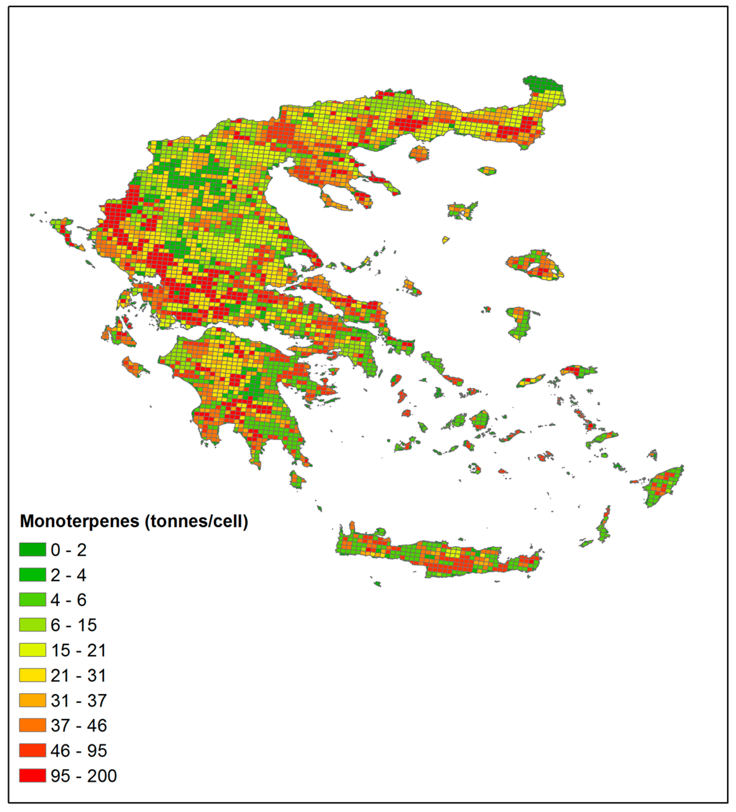
Month	Isoprene	Monoterpene	OVOCs
January	10.5	46.8	42.7
February	14.4	44.5	41.1
March	24.8	39.1	36.1
April	38.0	32.4	29.6
May	44.2	29.3	26.5
June	52.0	25.1	22.9
July	53.6	24.4	22.0
August	52.3	25.1	22.6
September	44.7	29.1	26.2
October	30.7	36.5	32.8
November	22.0	41.2	36.8
December	10.3	47.0	42.7

). On the other hand, in January, monoterpenes’ contribution is the highest one (46.8%), followed by OVOCs’ (42.7%) and isoprene’s (10.5%).

The temperature- and light dependency of the biogenic emissions determine their magnitude. This leads to an increase of BVOC emissions during the daytime, with observed maximum values at midday. For that reason, the sum above Greece of isoprene, monoterpene, and OVOCs daily emissions was calculated. As we can observe (Figure 6), isoprene emissions occur only during daytime because of their strong light dependency, as suggested by [12], while on the other hand, monoterpene and OVOCs emissions occur both during daytime and nighttime. The maximum values are observed during midday (13.00 UTC), with isoprene being the most abundant of the species.

A part of this study is the comparison between the annual biogenic emissions with the anthropogenic ones. For Greece, several studies have been done in order to estimate the anthropogenic NMVOCs emissions due to their importance in the creation of photochemical pollution. The annual anthropogenic NMVOCs emissions were derived from the study [5] concerning the years 2006 to 2012. For the comparison, the emissions for the year 2012 were used. The annual biogenic emissions were estimated up to 472 kt, and the anthropogenic ones up to 325 kt for Greece. We observe that the annual biogenic emissions exceed the anthropogenic emissions by a factor of 1.45, a fact that underlines the study of the biogenic emissions in the Mediterranean.

The total BNMVOCs emissions over the study area are estimated to be 473 kt, consisting of 220 kt of isoprene, 132 kt of monoterpenes, and 120 kt of OVOCs. Comparing the present results with those of other studies for Greece or for an extended area including Greece, it was found that our results differ by a factor of 0.58 from the results of [9], and by a factor of 1.92 from the study of [20]. A more detailed comparison was attempted with results from the application of the MEGAN model performed by [21] referring to 2011, over Greece. As can be seen by Figure 7 below depicting isoprene emissions at 12:00 UT, MEGAN produces the highest values at the same areas of Greece as does the present work. Moreover, computed isoprene values from specific cells were compared from 5:00 to 16:00 UT (

Table 3. Comparison between the hourly isoprene emissions derived from [21] (MEGAN) and from the present work concerning the month of September.

Time (UT)	Mitilene Island		Mount Parnitha		Kalamata
	MEGAN	This Work	MEGAN	This Work	MEGAN	This Work
5:00	0.4517	2.9428	0.1052	1.6083	0.2400	1.7286
6:00	1.1784	4.4107	0.3770	2.6558	0.8125	2.8487
7:00	1.9918	5.7848	0.6786	3.3429	1.3987	3.6122
8:00	2.9012	6.8139	0.9886	3.8856	2.0378	4.2774
9:00	3.7761	7.7954	1.2923	4.3828	2.5964	4.8008
10:00	4.4177	8.6426	1.4921	4.7437	2.9047	5.1691
11:00	4.7303	9.2528	1.5702	4.9988	2.9818	5.2909
12:00	4.5271	9.3756	1.4915	4.8454	2.6724	5.2071
13:00	3.9158	9.3631	1.3166	4.7316	2.0577	5.0542
14:00	2.8421	8.6822	0.9882	4.3925	1.5332	4.5949
15:00	1.4652	6.7755	0.5508	3.4415	0.9130	3.6578
16:00	0.3887	0.6073	0.1916	0.5165	0.3537	0.5730

). The relevant agreement between the results of this work and MEGAN is quite satisfactory considering the fact that the grid resolution is different as well as the reference year. It indicates that our values are higher by a factor of about 2, and given the fact that the estimated uncertainty level of annual global biogenic emissions is a factor of 3 [1], which is the lower limit of accuracy of annual biogenic emissions for Europe, it was assumed that the results from this study are in good agreement with already existing studies.

4. Concluding Remarks

In the present study, the biogenic emissions in Greece were estimated with the aid of a Geographic Information System (GIS), existing equations and detailed meteorological and solar radiation data. Hourly, daily, and annual isoprene, monoterpene, and OVOCs emissions were estimated for the area under study with a spatial resolution of 6 × 6 ${\mathrm{km}}^2$.

In the study domain, annual biogenic NMVOCs emissions were estimated to 472 kt, composed of 46.6% isoprene, 28% monoterpenes, and 25.4% OVOCs. The annual cycle of biogenic emissions is characterized by higher values during summertime which is in agreement with the influence of high temperature and solar radiation values on the emissions. It is estimated that 89.3% of the annual isoprene emissions occur between May and September due to their dependency on temperature and radiation fluxes. On the other hand, the corresponding percentages for monoterpenes and OVOCs are lower (75% for both types of hydrocarbons).

As it was expected, the different land-use categories emit different quantities of hydrocarbons as they are characterized by different foliar biomass densities and emission potentials. It was observed that the areas exhibiting peak isoprene emissions are covered either by forest with broadleaved deciduous trees or by forest with evergreen and deciduous trees, mostly present in western and northern Greece. Annual isoprene emissions contribute 46.3% to the annual biogenic emissions. Concerning the monoterpene emissions, the areas emitting the most are covered by forests with evergreen and deciduous trees. The annual monoterpene emissions contribute 28.2% to the total annual emissions. Finally, the annual OVOCs emissions are estimated to contribute 25.5% to the total annual emissions.

Further work has to be done concerning the estimation of biogenic emissions. More precisely, the use of isoprene, monoterpene, and OVOCs emission potentials is accompanied by a high level of uncertainty. In the present study, the emission potentials were derived from the database given by [17], which was the most recent study for the European vegetation since previous studies used. Already existing databases are based on the American vegetation types. Then, for the land-use categories characterized by a combination by two or more ecosystems, we do not have a certain emission potential. Therefore, more work is required for these land-use categories for Europe and more precisely, for the Mediterranean regions, as this area contributes significant to the total European annual biogenic emissions. Furthermore, the use of a fixed emission potential for the OVOCs emissions, due to lack of experimental measurements concerning the OVOCs, is a source of uncertainty.

Concerning the foliar biomass densities used for each month covering one year, it is underlined that they are, also, a source of uncertainty because of the use of corrective factors in order to describe the seasonal variation of the foliar biomass densities. Concerning the satellite land-use data, despite the fact that they are characterized by high resolution, they can be easily misinterpreted. In the present study, the satellite land-use data were checked and tested for the valid representation of land-use categories covering Greece. At this point, it should be mentioned that hourly meteorological data have been used for certain periods, instead of climatological data, affecting our estimations, a fact which reduces the uncertainty in the calculation of the environmental correction factors.

In conclusion, given the importance of biogenic emissions in atmospheric photochemistry in Greece, it is essential to continuously monitor, record, and improve the methods estimating the emissions from natural sources as well as the study of their interaction with the anthropogenic emissions and finally, their overall contribution to ozone, and to aerosols matter formation.

References

- Guenther, A.; Hewitt, C.N.; Erickson, D.; Fall, R.; Geron, C.; Graedel, T.; Harley, P.; Klinger, L.; Lerdau, M.; McKay, W. A global model of natural volatile organic compound emissions. J. Geophys. Res. Atmos. 1995, 100, 8873–8892. [Google Scholar] [CrossRef]
- Poupkou, A.; Giannaros, T.; Markakis, K.; Kioutsioukis, I.; Curci, G.; Melas, D.; Zerefos, C. A model for European Biogenic Volatile Organic Compound emissions: Software development and first validation. Environ. Model. Softw. 2010, 31, 45–56. [Google Scholar] [CrossRef]
- Piccot, S.D.; Watson, J.J.; Jones, J.W. A global inventory of volatile organic compound emissions from anthropogenic sources. J. Geophys. Res. Atmos. 1992, 97, 9897–9912. [Google Scholar] [CrossRef]
- Curci, G.; Beekmann, M.; Vautard, R.; Smiatek, G.; Steinbrecher, R.; Theloke, J.; Friedrich, R. Modelling study of the impact of isoprene and terpene biogenic emissions on European ozone levels. Atmos. Environ. 2009, 43, 1444–1455. [Google Scholar] [CrossRef]
- Fameli, K.-M.; Assimakopoulos, V.D. The new open flexible emission inventory for greece and the greater athens area (fei-gregaa): Account of pollutant sources and their importance from 2006 to 2012. Atmos.Environ. 2016, 137, 17–37. [Google Scholar] [CrossRef]
- Geron, C.D.; Guenther, A.B.; Pierce, T.E. An improved model for estimating emissions of volatile organic compounds from forests in the eastern united states. J. Geophys. Res. Atmos. 1994, 99, 12773–12791. [Google Scholar] [CrossRef]
- Naik, V.; Delire, C.; Wuebbles, D.J. Sensitivity of global biogenic isoprenoid emissions to climate variability and atmospheric co2. J. Geophys. Res. Atmos. 2004, 109. [Google Scholar] [CrossRef]
- Staudt, M.; Seufert, G. Light-dependent emission of monoterpenes by holm oak (Quercus ilex L.). Naturwissenschaften 1995, 82, 89–92. [Google Scholar] [CrossRef]
- Symeonidis, P.; Poupkou, A.; Gkantou, A.; Melas, D.; Yay, O.D.; Pouspourika, E.; Balis, D. Development of a computational system for estimating biogenic nmvocs emissions based on gis technology. Atmos. Environ. 2008, 42, 1777–1789. [Google Scholar] [CrossRef]
- Guenther, A.; Greenberg, J.; Harley, P.; Helmig, D.; Klinger, L.; Vierling, L.; Zimmerman, P.; Geron, C. Leaf, branch, stand and landscape scale measurements of volatile organic compound fluxes from us woodlands. Tree Physiol. 1996, 16, 17–24. [Google Scholar] [CrossRef] [PubMed]
- Bossioli, E.; Tombrou, M.; Karali, A.; Dandou, A.; Paronis, D.; Sofiev, M. Ozone production from the interaction of wildfire and biogenic emissions: A case study in Russia during spring 2006. Atmos. Chem. Phys. 2012, 12, 7931. [Google Scholar] [CrossRef]
- Liakakou, E.; Vrekoussis, M.; Bonsang, B.; Donousis, C.; Kanakidou, M.; Mihalopoulos, N. Isoprene above the Eastern Mediterranean: Seasonal variation and contribution to the oxidation capacity of the atmosphere. Atmos. Environ. 2007, 41, 1002–1010. [Google Scholar] [CrossRef]
- Kaltsonoudis, C.; Kostenidou, E.; Florou, K.; Psichoudaki, M.; Pandis, S.N. Temporal variability and sources of VOCs in urban areas of the eastern Mediterranean. Atmos. Chem. Phys. 2016, 16, 14825. [Google Scholar] [CrossRef]
- Guenther, A.B.; Monson, R.K.; Fall, R. Isoprene and monoterpene emission rate variability: Observations with eucalyptus and emission rate algorithm development. J. Geophys. Res. Atmos. 1991, 96, 10799–10808. [Google Scholar] [CrossRef]
- Guenther, A.; Zimmerman, P.; Wildermuth, M. Natural volatile organic compound emission rate estimates for us woodland landscapes. Atmos. Environ. 1994, 28, 1197–1210. [Google Scholar] [CrossRef]
- Fameli, K.-M.; Assimakopoulos, V.D.; Kotroni, V. A Modelling Study of the Photochemical and Particulate Pollution Characteristics above a Typical Southeast Mediterranean Urban Area; Institute for Environmental Research and Sustainable Development: Thessaloniki, Greece, 2015; p. 36. [Google Scholar]
- Steinbrecher, R.; Smiatek, G.; Köble, R.; Seufert, G.; Theloke, J.; Hauff, K.; Ciccioli, P.; Vautard, R.; Curci, G. Intra-and inter-annual variability of voc emissions from natural and semi-natural vegetation in europe and neighbouring countries. Atmos. Environ. 2009, 43, 1380–1391. [Google Scholar] [CrossRef]
- Taylor, M.; Kosmopoulos, P.; Kazadzis, S.; Keramitsoglou, I.; Kiranoudis, C. Neural network radiative transfer solvers for the generation of high resolution solar irradiance spectra parameterized by cloud and aerosol parameters. J. Quant. Spectrosc. Radiat. Transf. 2016, 168, 176–192. [Google Scholar] [CrossRef]
- Kosmopoulos, P.G.; Kazadzis, S.; Taylor, M.; Raptis, P.I.; Keramitsoglou, I.; Kiranoudis, C.; Bais, A.F. Assessment of surface solar irradiance derived from real-time modelling techniques and verification with ground-based measurements. Atmos. Meas. Tech. Discuss. 2017. [Google Scholar] [CrossRef]
- Simpson, D.; Winiwarter, W.; Börjesson, G.; Cinderby, S.; Ferreiro, A.; Guenther, A.; Hewitt, C.N.; Janson, R.; Khalil, M.A.K.; Owen, S. Inventorying emissions from nature in europe. J. Geophys. Res. Atmos. 1999, 104, 8113–8152. [Google Scholar] [CrossRef]
- Bossioli, E.; Tombrou, M.; Kalogiros, J.; Allan, J.; Bacak, A.; Bezantakos, S.; Mihalopoulos, N. Atmospheric composition in the Eastern Mediterranean: Influence of biomass burning during summertime using the WRF-Chem model. Atmos. Environ. 2016, 132, 317–331. [Google Scholar] [CrossRef]