1. Introduction
The use of unmanned aerial systems (UAS), often also called remotely-piloted aircraft systems (RPAS), for atmospheric research has increased significantly over the last few decades. The new setup of ALADINA (Application of Light-weight Aircraft for Detecting in situ Aerosols) in the context of the ongoing development is provided as an introduction to the current modifications. The first applications date back to several decades ago [
1]; later, some UAS applications of atmospheric research groups were reported in the 1990s [
2]. Compared to these first meteorological applications, there has been a revolution concerning the functionality, size and complexity of even commercially available airborne systems, autopilots and the corresponding hardware and software. Nowadays, UAS are deployed in a broad range of meteorological research fields. The smallest systems with a weight below or slightly exceeding 5 kg are mainly equipped with basic meteorological sensors for measuring humidity and temperature [
3]. They can be used comparable to a recoverable radiosonde [
4], but have the advantage of performing specific flight patterns, as demonstrated by Hemingway et al. [
5], which shows the repeated sampling and analysis of the small-scale atmospheric boundary layer (ABL) phenomena with a multicopter system. Some systems provide measurements of additional parameters, e.g., ozone concentration [
6] or the concentration of the greenhouse gases methane and carbon dioxide [
7].
There have been significant improvements in the sensors for estimating the basic meteorological parameters. For determining the three-dimensional wind vector in high temporal and high spatial resolution, a miniaturized multi-hole probe (MHP) along with the Global Navigation Satellite System (GNSS) and inertial measurement unit (IMU) has been implemented [
8,
9,
10]. Using these systems, turbulence parameters can be studied [
11] and turbulent fluxes of sensible heat are derived [
12]. Other systems use specific flight patterns and assumptions of the influences of wind on UAS to provide an estimate of the wind speed and wind direction in order to derive turbulent fluxes of sensible and latent heat [
13,
14].
In addition to basic meteorological parameters at high resolution, several systems with a payload weight between 5 and 25 kg rely on miniaturized sensors for measuring aerosol properties. A condensation particle counter in combination with a three-wavelength absorption photometer and chemical sampling has been used by Bates et al. [
15]. Another research work includes measurements of longwave and shortwave broadband radiation, total aerosol particle number concentration and size distribution, as well as a video camera [
16].
Applications of UAS and meteorological payload are manifold. Various systems have been deployed to study atmospheric particles at different locations. Bates et al. [
15] reported measurements at Ny-Ålesund, Svalbard, for studying long-range transport of particles into the Arctic, especially black carbon (BC). The system of de Boer et al. [
16] has been developed to study Arctic haze properties in the Alaskan Arctic. Furthermore, applications to perform measurements in thunderstorms and tornadic supercells have been reported [
17].
Besides typical short-term missions of meteorologically-equipped systems, other UAS with combustion engines provide the capability of long-range flights, as far as permitted by the authorities. Therefore, they mostly are operated in sparsely-inhabited areas. Such systems have been used for up to 30 h per flight in the Arctic [
18], Antarctic [
19] and above the Indian Ocean [
20]. In addition to the meteorological sensors, remote sensors are employed for monitoring surface properties like ice cover, sea ice type and surface temperature [
18].
The next step in the complexity of operations is the simultaneous use of more than one UAS, reported in Ramanathan et al. [
20], who coordinated three aircraft measuring total aerosol particle number concentration, soot and radiation related to clouds. UAS operation with two aircraft following different flight patterns was performed as well in the study of Platis et al. [
21]. For some meteorological experiments, the advantages of UAS and manned aircraft were combined to complete the overall picture (e.g., Neininger and Hacker [
22], Lothon et al. [
23]). A recent overview of UAS application for meteorological research and their instrumentation is provided by Elston et al. [
24] and Villa et al. [
25].
Compared to other platforms, UAS fill a gap between stationary in situ and remote sensing measurement systems like ground-based LiDAR and radar or tethered balloon observations, on the one hand, and on the other hand, manned aircraft, which cover larger distances at higher cruising speed. For repeatedly probing the development of the atmospheric boundary layer on small scales of a few kilometers, UAS are the most cost-efficient and easy to operate devices available. With the ongoing miniaturization of meteorological sensors and electronic components, they achieve the same temporal resolution as in situ observations onboard manned aircraft, and complex light-weight instruments can be included. Additionally, UAS provide the possibility to probe areas too hazardous for manned measurement flights, e.g., in volcanic ash conditions or over sites contaminated by ionizing radiation. Since they fly generally at lower cruising speed (typical 10–30 ms), the spatial resolution is higher compared with manned aircraft (typical cruising speed 50–200 ms) assuming the identical measurement rate.
The UAS ALADINA (Application of Light-weight Aircraft for Detecting in situ Aerosols; the principal shape of the aircraft can be seen in [
26]) operated at the Institute of Flight Guidance at TU Braunschweig (Technische Universität Braunschweig) corresponds to the weight class up to 25 kg with a wing span of 3.6 m. The pusher aircraft of type Carolo P360 was designed with the purpose to carry large sensors (sensor volume up to 0.02 m
) in a specifically-designed payload bay. To avoid contamination, influence on aerosol measurements and to reduce vibrations, it is electrically powered. The first setup of the UAS ALADINA has already been described in detail [
26]. As the measurement system has undergone significant changes and improvements after several extended field experiments [
21,
26], the current system with additional instrumentation, the new data acquisition system deployed in the project Dynamics-aerosol-chemistry-cloud interaction in West Africa (DACCIWA) [
27,
28] and careful sensor characterization are presented here.
The overall advantage of the UAS ALADINA is the broad range of sensors installed. Since the research group developing and operating ALADINA has its background in the operation of the Meteorological Mini Aerial Vehicle (M
AV, [
11,
12,
29,
30]) and the operation of the manned research aircraft D-IBUF [
31] and its measurement systems and works closely together with the researchers developing and using the Multi-purpose Airborne Sensor Carrier (MASC, [
32,
33,
34], ALADINA takes advantage of many experiences with those systems and subsystems.
For ALADINA, a preview of the resulting parameters and uncertainties can be found in
Table 1, which will be discussed below.
2. Flight Operation for Atmospheric Research
The operation of the UAS ALADINA in the field requires flat terrain of approximately 50 × 5 m for takeoff and landing (grass, gravel, concrete) and two operators. One acts as a pilot for remotely-piloted takeoff and landing and supervising the flight guided by the autopilot. The second operator supervises the mission at a mobile ground station computer, checking the functionality of the autopilot, the sensors and the plausibility of data using a downlink, which provides preliminary real-time data with a transmission rate of currently 1 Hz to ensure a robust connection. It is limited by transmission bandwidth and signal power considering the power consumption, module weight and local transmission regulations. Access to electricity on site is not mandatory, but recommended in order to recharge the batteries of the aircraft and ground station. The limitation of the overall weight up to 25 kg is intended to minimize the administrative effort for flight permissions, since 25 kg currently states a threshold in operating rules (at least in European countries [
7]). The handling of ALADINA is done according to appropriate checklists adopted from professional manned-aircraft operation, to ensure that both the instrumentation and the aircraft functionality are checked and the system is ready for takeoff. After switching on the measurement electronics, the alignment of the magnetic sensor is performed. Through wireless communication, the onboard computer can be connected to the ground station, and the measurements can be remotely started by sending the appropriate command. Shortly after the manually-piloted takeoff, the autopilot is enabled, flying precisely along the uploaded waypoint list. The autopilot flight control is configured for more precise measurements rather than precise path following. That means constant speed control and altitude control are more important than the horizontal navigation control. Furthermore, there is no additional yaw control to provide continuous air flow on the sensors of the aircraft supported by the directional stability of ALADINA itself. Waypoints can be sent during flight to maintain maximal flexibility and to adopt the flight mission to the scientific task. The typical flight time is around 45 min, limited by the batteries for propulsion (2 × 10 s lithium polymer cells, each 10 Ah, overall capacity 740 Wh) and air temperature. After the manually-piloted landing, the typical turn-around time between two flights (including changing the batteries for propulsion, autopilot and payload, as well as copying the data) needs around 20 min. By recharging batteries in parallel with the flights, more than eight consecutive full duration flights on one day can be performed. In comparison with the original system [
26], position lights, which allow the determination of the aircraft attitude to fly safely in weak sunlight conditions or even at night, were newly installed. In addition, removable landing lights can support pilots in estimating height over ground while landing.
3. Validation Methods for UAS Measurements
Since measured and post-processed data have to be validated, it is of importance to discuss and improve validation methods critically due to continuous improvements of sensors and algorithms. Validation methods used by the ALADINA research team and other authors, e.g., [
9,
21,
26,
35,
36,
37], are summarized in this section regarding their usefulness before being applied on the dataset.
Error propagation calculations:
When calculating error propagation for real systems, the sensor errors and cross-sensitivities have to be known for each flying system. Normally, these values are not constant, but depend on the flight state. The needed sensor values are not given in manuals and datasheets in this detail, as manufacturers often do not know the special conditions of each applicant and provide error values derived from standardized laboratory tests. Error propagation calculation is therefore limited to deepen the knowledge about the system and to obtain total system uncertainty estimates based on sensor errors provided by manufacturers.
Laboratory tests:
Laboratory tests can be used for identifying sensor errors and cross-sensitivities that are not given by the manufacturer. Laboratory calibrations, however, normally do not cover the complete sensor environment during flight. Results are therefore not directly applicable to inflight measurements. As an example, wind tunnel calibrations of pressure probes do not include the flow field around the UAS. Even with the complete UAS installed in a wind tunnel, blockage and wall effects distort the result by a relevant magnitude. Investigating transient maneuvers like turns or the flight in free air turbulence in the laboratory is very expensive.
Numerical simulations:
Simulations can be used to get knowledge of principal sensor behavior, but it is important to include all relevant influences on the sensors in the model. There may remain some unknown influences (cross-correlations and error terms), which can possibly be identified by laboratory tests. Transient simulations of complex systems often require remarkable computational effort.
Comparison of independent sensors:
The comparison of sensors is used to determine the relative differences of the measurements. This comparison must take into account the degree of interdependency between the measurements, considering for instance the measurement task, the sensing principles and the spatial difference. Proclaiming one sensor as the reference requires an assured uncertainty about one magnitude below the expected uncertainty of the sensor that shall be assessed. Comparisons of inflight measurements with ground-based measurements are affected by the time- and position-dependent environment parameters; e.g., for three-dimensional LiDAR wind measurements, beam velocities of different beam directions are combined to obtain wind vectors and therefore only represent mean velocities over a certain volume (change in time), e.g., Weitkamp [
38].
Intrinsic plausibility tests:
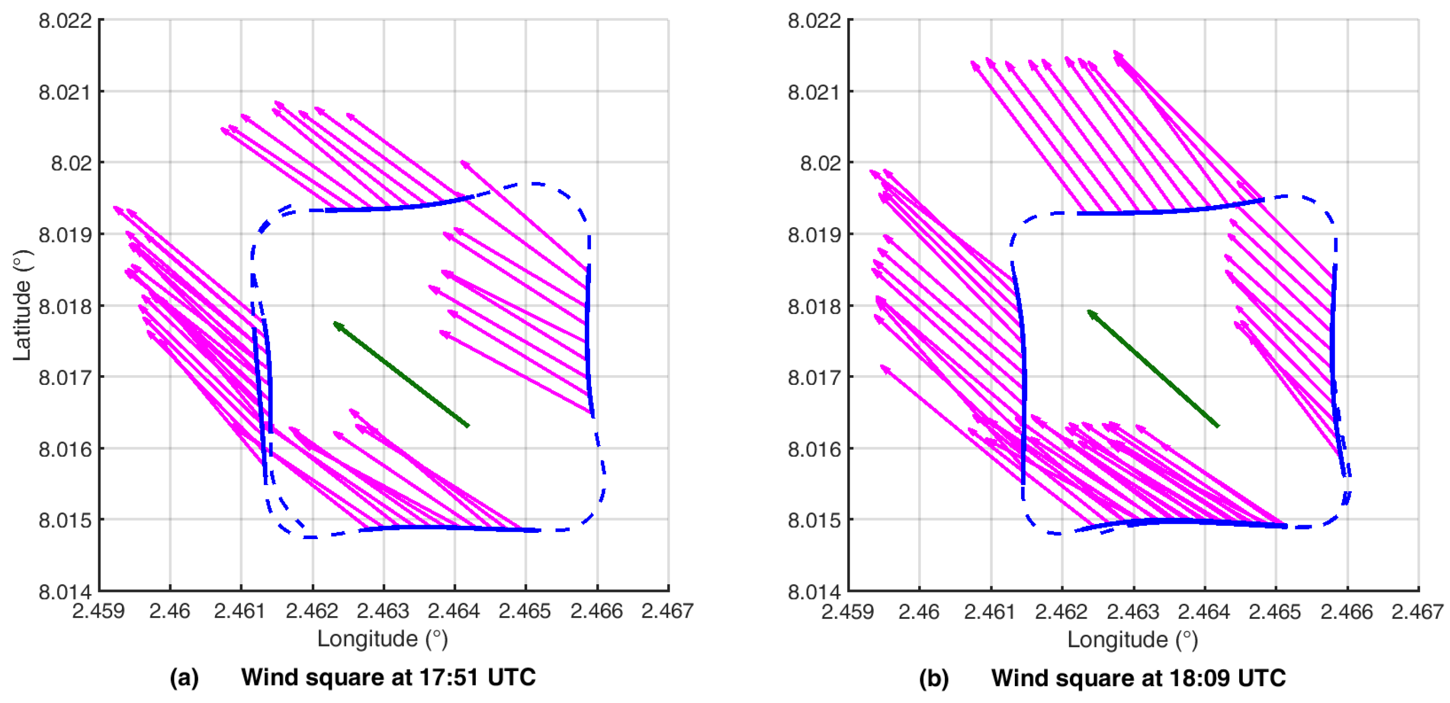
Intrinsic plausibility tests rely on the inflight dataset itself examining the theoretically zero correlation between physical independent values, e.g., static air temperature must be uncorrelated to the aircraft attitude, and the vertical wind component in the Earth-fixed reference frame must be uncorrelated to the aircraft phugoid (slow natural oscillation around the transverse aircraft axis resulting in a pitch oscillation) in straight flight. Other common flight maneuvers are repeated wind squares to demonstrate that the horizontal wind determination does not correlate with flight direction and flight speed. Furthermore, ascents, descents and general attitude changes can be used to show uncorrelated measurements. When using such plausibility tests, assumptions have to be made such as nearly constant wind fields or slowly-varying temperatures at identical heights. Furthermore, statistic methods could be used to prove significant independence of, e.g., flight maneuvers on measurements.
Model-based validation (e.g., Kolmogorov’s law):
The most favorite model for validating airborne meteorological data is the Kolmogorov law for the power of local isotropic turbulence in the inertial subrange [
39]. When using model-based validations, one should make sure that boundary conditions are given. As shown in several papers (e.g., Lampert et al. [
11]), the conditions (steady-state, locally isotropic) for the Kolmogorov law may not be given in daytime transition. This causal problem can be moderated by using data obtained in appropriate meteorological conditions. Finally, the compliance of measured turbulent values with the Kolmogorov law is a necessary, but not sufficient criterion.
4. Devices on the UAS ALADINA for Precise Monitoring of Boundary Layer Properties
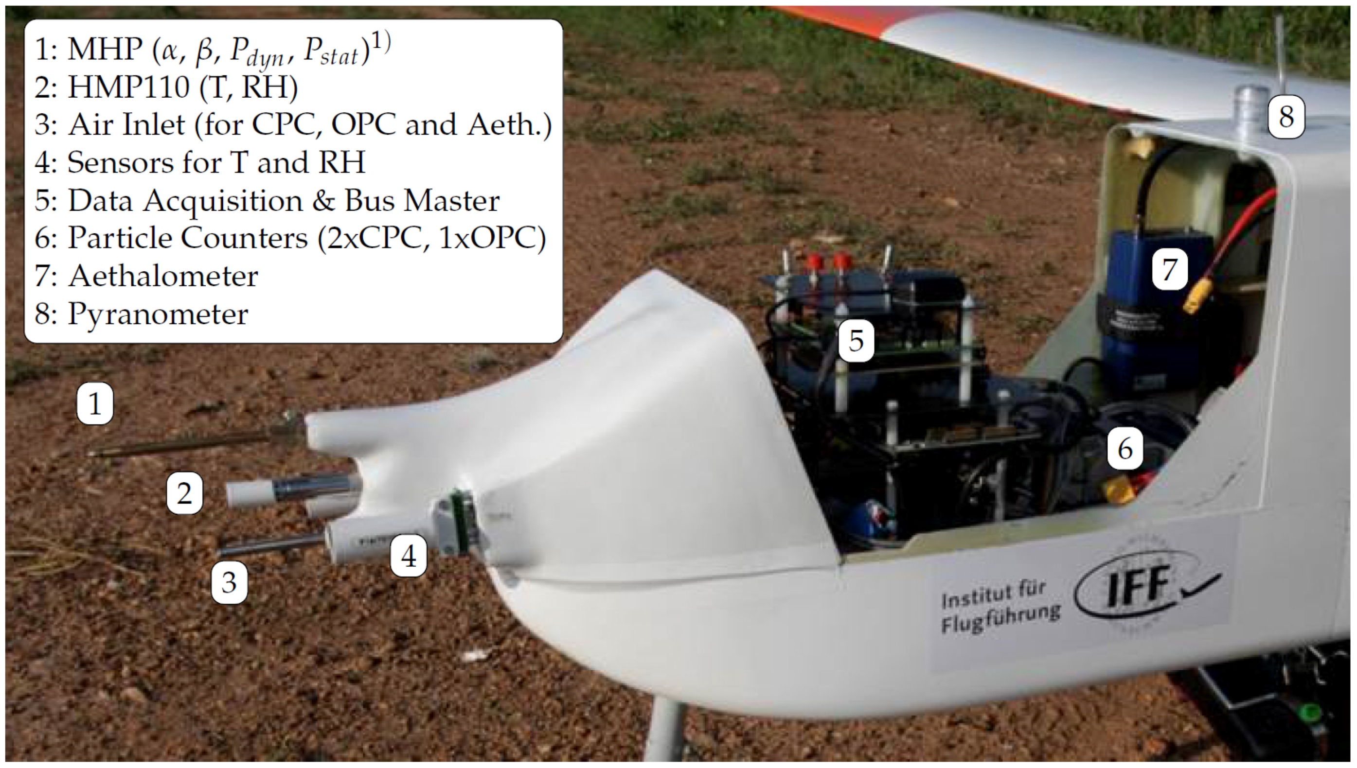
The new setup of the UAS ALADINA is shown in
Figure 1, where sensors and systems are marked and named.
A complete meteorological sensor package to determine turbulence data is installed in the nose of ALADINA. This sensor package was re-engineered taking advantage of experiences with the manned aircraft D-IBUF [
31], the UAS M
AV [
29], MASC [
10] and the sensor package installed in ALADINA before [
26]. Compared to the previous setup [
26], all sensor interfaces (circuit boards) were redesigned, special housings were added to temperature and humidity sensing elements to make them total air temperature probes known from manned aviation (cf.
Section 4.3.1 for more details), MHP tubing was changed, data acquisition changed completely and data processing was redesigned. Only airframe and particle counters remained identical; therefore, no comparison to the setup shown in [
26] is done.
In the following, the system to acquire data, the different sensors and the algorithms and procedures used to calculate the final parameters out of the raw data are presented.
To validate measured and derived data, validation methods presented in
Section 3 are applied. Temperature and humidity measurements are validated by comparing ascents with descents (intrinsic validation) and by regarding power densities in comparison with theoretical power density slopes (model-based validation). Wind vector plausibility is shown by a wind square, where no correlation between flight direction and wind direction and wind magnitude should be present (intrinsic test), whereas turbulence data plausibility is shown by comparing actual power density slopes with theoretical power density slopes (model-based validation). Total aerosol particle concentration is compared against ground-based measurements (comparison of independent sensors), whereas a profile of black carbon mass concentration measurements is shown (weak intrinsic validation). At the end, pyranometer data are improved by correcting the angle of sun incidence on the sensor caused by attitude (mostly roll) motion (weak intrinsic validation).
4.1. Data Acquisition and Data Bus System
The data acquisition is realized with a bus system consisting of several microcontroller boards with a direct sensor connection and one single-board computer (SBC). A 168-MHz clocked 32-bit microcontroller, based on the ARM Cortex M4 (ARM Limited, Cambridge, UK) architecture is the central part of the boards closely situated to the sensors. The hard real-time programmed microcontrollers capture the digital sensor data at a rate of 100 Hz. An analog sensor signal is acquired by the 24-bit sigma-delta analog-digital converters AD7190 (Analog Devices, Norwood, MA, USA) with a modulator frequency of 64 kHz. By use of its internal analog front-end and noise shaping downsampling filter set to an output data rate of 100 Hz, a noise free resolution of 18 bit can be achieved in the used configuration. The time stamping of the time critical data acquisition is provided by a GNSS-receiver. By signalizing the beginning of a second with a highly precise PPS-signal (pulse-per-second), the bus client microcontrollers are synchronized. The PPS-signal comes directly out of the GNSS-receiver (uBlox, Thalwil, Switzerland) with an accuracy of better than 10 s. Therefore, the influence of the temperature and the manufacturing of the oscillators on the different boards can be compensated. This allows one to timestamp the data with the precision of a fraction of 1 ms. The sensor data are transferred using a central bus system with a time division multiple access (TDMA) bus arbitration. The use of the EIA-485-A-1998 (Electronic Industries Alliance) standard for serial communication allows data rates of about 3.2 MBits and ensures a fail-safe transmission in an environment where electromagnetic interference cannot be excluded. The SBC reads the data on the bus lines and sequentially writes them on an SD-card. At the end of a flight, the data can be downloaded via an ftp-client over a wireless LAN connection, or the SD-card can be removed and read out on any computer. Online transcoding of the data stream on the SBC allows transmitting relevant data using an XBEE-module to the ground station with a rate of currently 1 Hz.
4.2. Positioning
Inflight position of ALADINA is measured using a miniature MEMS (micro electromechanical system)-based IMU (inertial measurement unit) with INS/GNSS (integrated navigation system/global navigation satellite system) data fusion iVRU (iMAR, St. Ingbert, Germany). Data are provided via serial transmission.
4.3. Temperature and Humidity
4.3.1. Sensors Installed for Temperature Measurements
Three different sensors are installed in the nose of the aircraft to measure temperature: the widely-used sensor of the type HMP110 (Vaisala, Vantaa, Finland), which is a Pt1000 element, a digital factory-calibrated-sensor of the type TSYS01 (Measurement Specialties, Hampton, VA, USA) and a fine wire sensor fabricated at the Institute of Flight Guidance, TU Braunschweig, completely redesigned based on experiences in [
32], are installed. The sensor consists of two measurement channels using 0.0125-mm platinum wires with one wire setup parallel and one wire setup perpendicular to the flow. As a result of the re-engineering of the fine wire sensor, it is well protected by a housing and was used reliably for the whole campaign of DACCIWA (Dynamics-aerosol-chemistry-cloud interaction in West Africa, Knippertz et al. [
27]) during more than 30 h of flight time without any break, despite the harsh dusty environment.
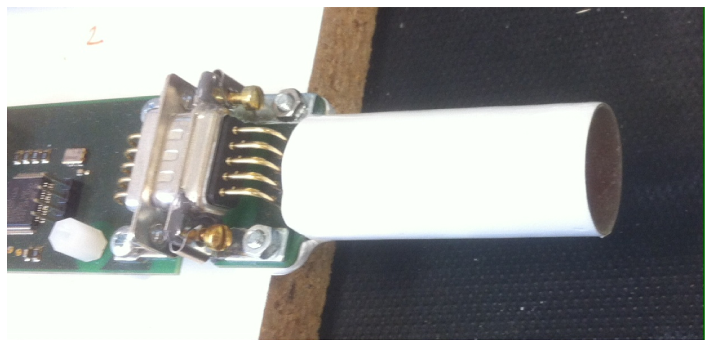
To achieve a well-defined sensor environment, housings acting as nozzles have been installed around the temperature and humidity sensing elements. This leads to total pressure conditions granting enough through-flow by an aspect ratio between inflow and outflow area of 1:5. The aspect ratio in combination with the roughness of the sensor circuit board was shown to result in nearly total pressure conditions (more than 90% of total pressure) and flow speeds inside the nozzle of about 20% of the undisturbed flow speed to allow fast measurements by the sensors. This technique is very common for temperature probes mounted on manned aircraft, e.g., the temperature sensor Rosemount Model 101 F. As an example, the nozzle of a temperature sensor can be seen in
Figure 2.
4.3.2. Sensor Fusion of Temperature Measurements
To characterize the ABL, static temperatures are needed, which are temperatures corrected for the warming effect of increased pressure at the sensor’s site. Taking into account the dynamic pressure, static values (e.g., static temperature) can be derived accurately from the measured total values. The data of these three sensors can be fused to get both reliable absolute temperature measurements and fast fluctuations.
The relation between total air temperature and static air temperature (both in Kelvin) is given by Equation (
1):
where
(=1.4) denotes the ratio of the heat capacity at constant pressure to the heat capacity at constant volume and
denotes the Mach number (both dimensionless quantities).
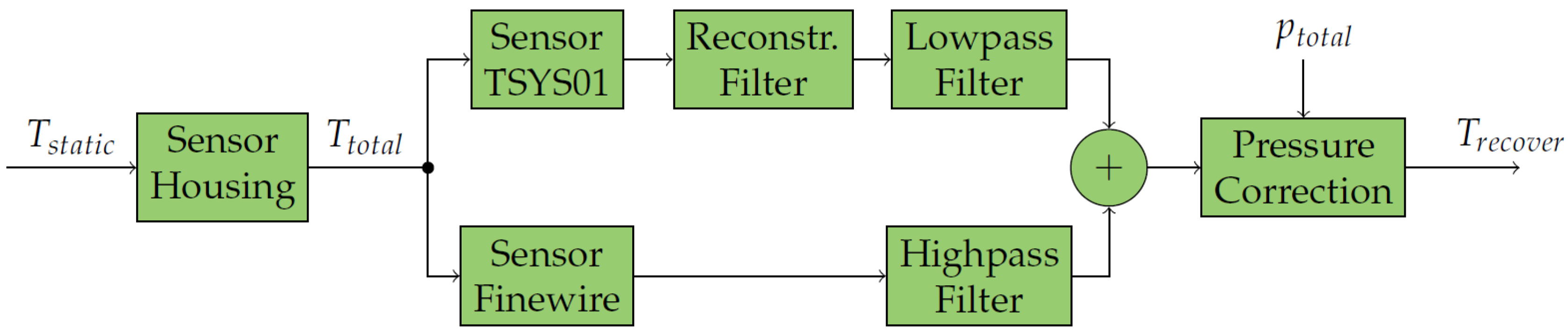
Complementary filtering is used for fine wire and the factory calibrated readings of the TSYS01 after removing the phase lag. HMP110 sensor readings are only available every second; they were not used for the complementary filtering. Analog output is also available, but the response time is expected to be in the range of the capacitive humidity sensor to allow dew point estimation. Nevertheless, HMP110 temperature measurements can be used as a redundant source. Complementary filtering is done by combining high- and low-pass (Butterworth type, both of first order) filtered measurements. To remove the heat capacity-caused phase lag before on the TSYS01 data, a system with a transfer function of first order is assumed, and readings are filtered with the inverse transfer function. The cutoff frequency of the complementary filters should be lower than the cutoff frequency of the assumed first order system for the reconstruction filter; otherwise, noise may be amplified. The whole process is illustrated by
Figure 3.
The cutoff frequencies and time constants to filter complementarily and remove phase lag can be derived by taking into account sensor response times (dynamic behavior), which can be determined by comparing ascents and descents or by using more sophisticated techniques, e.g., presented by Tagawa et al. [
40].
When two systems with a transfer function of first order and differing time constants can be assumed, every transfer function
, where
s denotes the complex frequency domain parameter, only contains one configuration parameter: the time constant
. Since the air temperature is unknown and has to be recovered, these equations cannot be solved directly. The technique presented in [
40] solves these two dynamic equations by assuming the same
for both sensors and hence minimizes the mean square difference
of the retrieved air temperature in the frequency domain.
The sensors used showed broad overlap in reliable spectral bands; extracted air temperature therefore consists of the low frequencies measured by the factory-calibrated temperature sensor TSYS01 and the fluctuations recorded by the fast responding fine wire sensor. Errors propagated through the algorithm are attenuated by the applied filters.
4.3.3. Sensors Installed for Humidity Measurements
For humidity measurements, different sensors of the same measuring principle (capacitive) were used, each carefully integrated in a well-defined environment (total pressure conditions with a sufficient flow rate;
Figure 2). One is of the type HMP110 (Vaisala, Vantaa, Finland), which is commonly used [
41] and often referred to, and a sensing element Rapid P14 (Innovative Sensor Technology, Ebnat-Kappel, Switzerland).
In very humid conditions (RH > 90%), it was shown to be mandatory to seal sensors and electronics close to sensors (e.g., capacitance to digital converters (CDC)) with conformal coating against condensation and water droplets. This allows measuring relative humidity up to 95% at temperatures of about 20 °C without losing accuracy or temporal response. Without sealing, water may influence the overall capacity of the sensor electronics. In more humid conditions, the capacitive measuring principle will not work properly.
4.3.4. Post-Processing of Humidity Measurements
The sensor P14 has been well investigated in Wildmann et al. [
42], where a technique has been shown to reconstruct water vapor on the sensor surface by taking advantage of physical modeling. Furthermore, the limitations of this technique have been shown in Wildmann et al. [
42]. Because of these limitations, again a first order transfer function for humidity measurements is assumed, and ascents and descents were compared to determine time constants. Since the datasheet describes longer response times for decreasing humidity, one could take into account two time constants: time constant
for increasing humidity and time constant
for decreasing humidity. Complementary filtering (cf.
Section 4.3.2) with the long-term stable HMP110 readings and the Rapid P14 data for fluctuations has been performed.
4.3.5. Validation of Temperature and Humidity Results
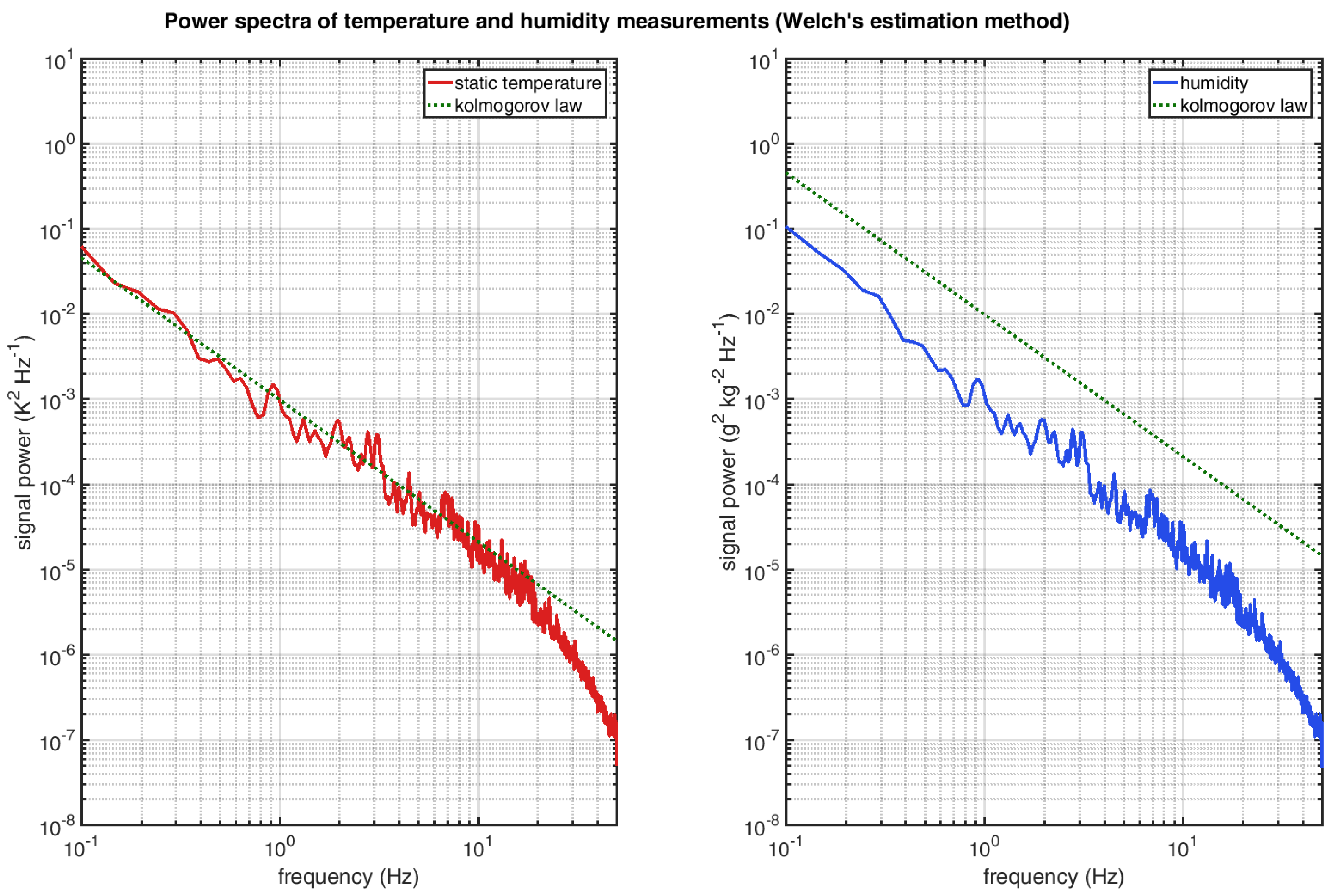
To check for reliability,
Figure 4 shows the power spectra of the sensors used (on the left side temperature, on the right side humidity as the mixing ratio). The power spectra were calculated using the method of Welch [
43]. Complementary combined sensor data fit well to the
power law up to 25 Hz for temperature readings. Since calculation of the mixing ratio depends on temperature, it is shown that relative humidity readings at least do not compromise the spectrum slope. Spectra of relative humidity do not have to follow the
power law in locally isotropic turbulence in the inertial subrange [
39]; therefore, the mixing ratio is used for the spectral roll-off.
To prove reliability, ascents can be compared with descents in the same area, assuming that ABL properties do not change significantly during the time needed for consecutive vertical profiles.
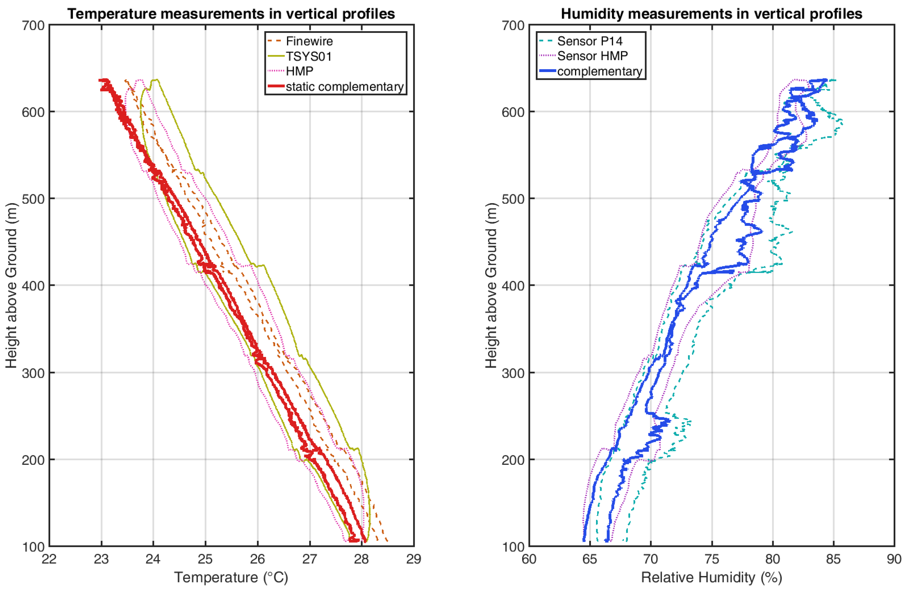
Figure 5 (left) shows vertical profiles (ascent with following descent) to prove that no drift and no lag occurs in the retrieved “best guess” temperature after complementary filtering. The phase lag of both HMP110 and TSYS01 can be seen in the top region of the profile around 800 m, where raw measurements describe a smooth curvature around the sharp switch between ascent and descent. Fine wire measurements are not affected by this: indeed, minimal drift can be observed over hours (less than 0.5 K per hour). Therefore, the complementary combined total temperature can be easily converted into a static air temperature with an accuracy of better than 0.1 K. The offset between measurements of the HMP110 and the TSYS01 of 0.2 K has its origin in a pending calibration implementation in the data processing.
Figure 5 (right) shows vertical profiles to check data qualitatively against accuracy and phase lag for humidity measurements. Since time constants of the HMP110 and the Rapid P14 sensor only differ minimally and humidity fluctuated fast due to cloud fractions, a phase lag can not be observed in the plot. In both subfigures, it can be seen that raw measurements of slowly-responding sensors depend on the flight pattern, since the ascents and descents were flown by doing turns at constant altitudes followed by straight ascent/descent legs. Complementary filtered values and fast-responding sensors do not inherit these errors.
4.4. Wind and Turbulence Measurements
4.4.1. MHP to Determine Static Pressure, Dynamic Pressure, Angle of Attack and Angle of Sideslip
A multi-hole probe is installed to determine sideslip angle and angle of attack, airspeed and barometric height. The MHP is calibrated in the wind tunnel with the complete front part of the fuselage of ALADINA (cf.
Figure 1), and errors induced by the fuselage are therefore already included in the calibration.
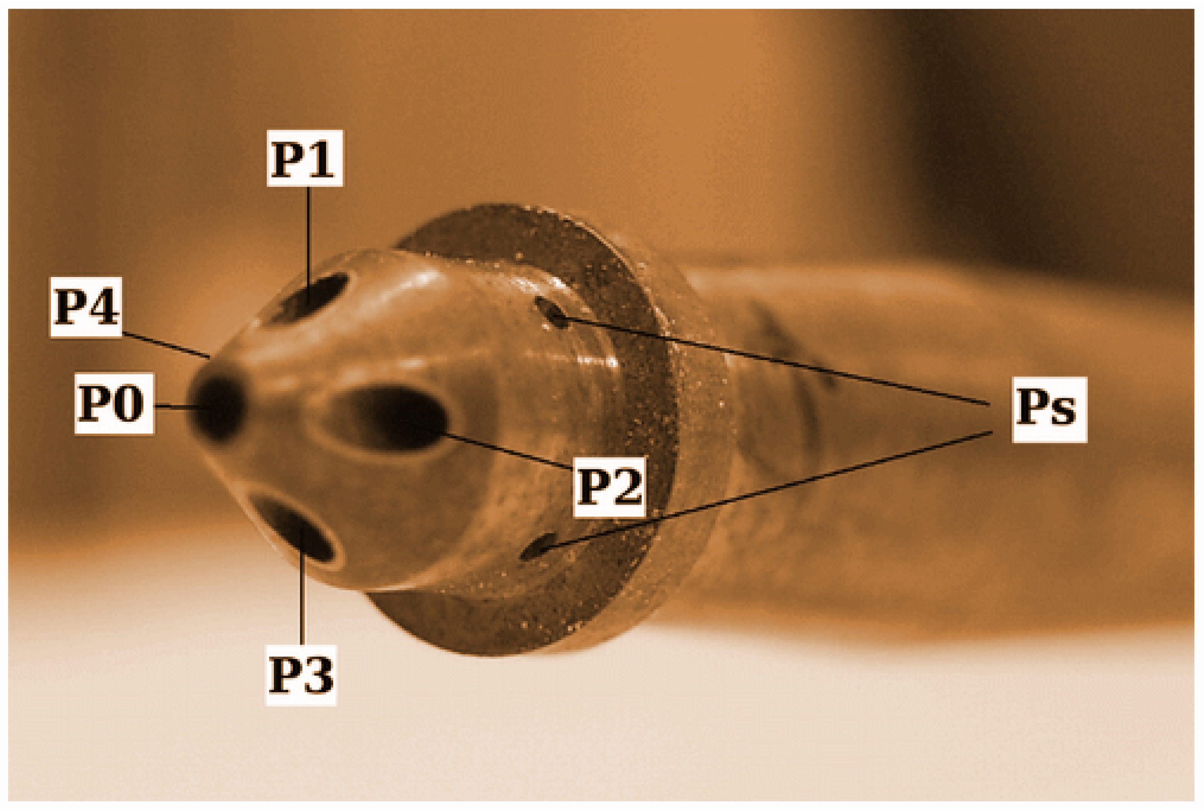
In ALADINA, a miniaturized conical multi-hole probe (MHP) deployed for other different UAS (e.g., Wildmann et al. [
10] and Martin et al. [
30]) is used to derive dynamic pressure, static pressure, sideslip angle and angle of attack to be able to determine the wind vector. This MHP and its pressure ports are shown in
Figure 6. In very humid conditions, small droplets may corrupt measurements of the MHP.
4.4.2. Vector Difference Wind Determination
Raw measurements of the multi-hole probe can be transformed to angle of attack, angle of sideslip, static and dynamic pressure using wind tunnel calibration. Combined with the measured angles of the installed INS/GNSS system, the wind vector with an accuracy of 0.5 ms
in components at a data rate of 25 Hz is derived according to the formulation shown by Lenschow [
44]. The fundamental vector difference equation is:
where
denotes the wind vector,
the flight path velocity and
the velocity vector of the aircraft with respect to the air, all three vectors in geodetic coordinates.
Different from the pressure wiring in [
8,
33], for the new setup of ALADINA, pressure differences from oppositely located holes in the cone of the MHP (
,
) are measured directly. The same setup was used by Reineman et al. [
45] and other airborne systems [
31]. To determine true airspeed, the total pressure at the front hole is measured against the static pressure port (
). Short pressure tubes (length < 200 mm) shift resonance effects towards higher, extraneous frequencies (
> 100 Hz). Using this setup, only three difference pressure sensors and one absolute pressure sensor (for the static pressure) are needed.
4.4.3. Enhanced Wind Determination Using Complete Flow Angle Calibration
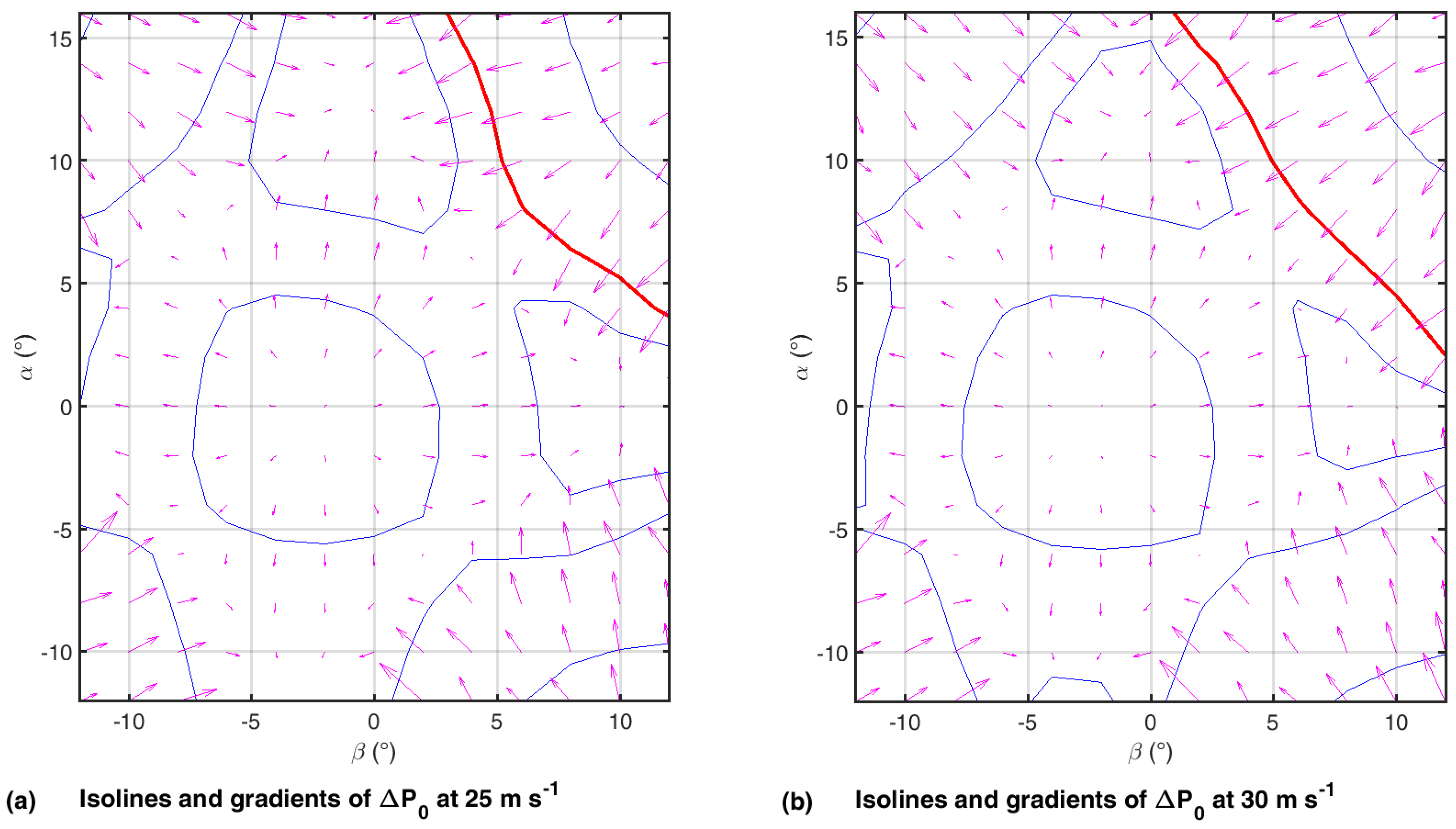
Small MHP often show discontinuities and non-linear behavior. Normalization to dimensionless pressure coefficients therefore reduces accuracy, since calibration field dependencies on dynamic pressure are neglected. An example of such a calibration field where normalization is not valid is shown in
Figure 7. In this figure, vector gradients of the calibration fields for two different calibration TAS (true air speed), 25 ms
(
Figure 7a) and 30 ms
(
Figure 7b), are shown. Since normalization does only affect gradient vectors in value, gradient vector directions have to be identical to allow normalization; this is not the case for the installed probe regarding gradient direction arrows and emphasized isoline curvature in the first quadrant of
Figure 7a,b; therefore, normalization would lead to degraded wind vector results.
Normalization reduces the three dimensions of a volumetric measurement field, e.g.,
, into a two-dimensional field
to improve the comprehension of angle measurements. Instead of deriving polynomials only dependent on two (normalized) measurements, one can also derive polynomials in a three-dimensional field. It is not mandatory to use algebraic expression over the whole definition area; a local projection between calibrated values (also known as interpolation) is adequate with respect to other uncertainties in wind vector measurements (e.g., pressure transducers, aircraft attitude). When the measured calibration volume to define the projection between angles and measured pressures (Equation (
3)):
is bijective (each element of the left-hand set is paired with exactly one element of the right-hand set and vice versa), which is satisfied by any appropriate design of a calibratable MHP (strong continuous gradients for
,
and
), it is possible to build the inverse function
. This can also be done using algebraic expressions, but much more simply by gridding data in order to generate a directly interpolatable volumetric data field as shown in Equation (
4).
The resulting subsets
, e.g.,
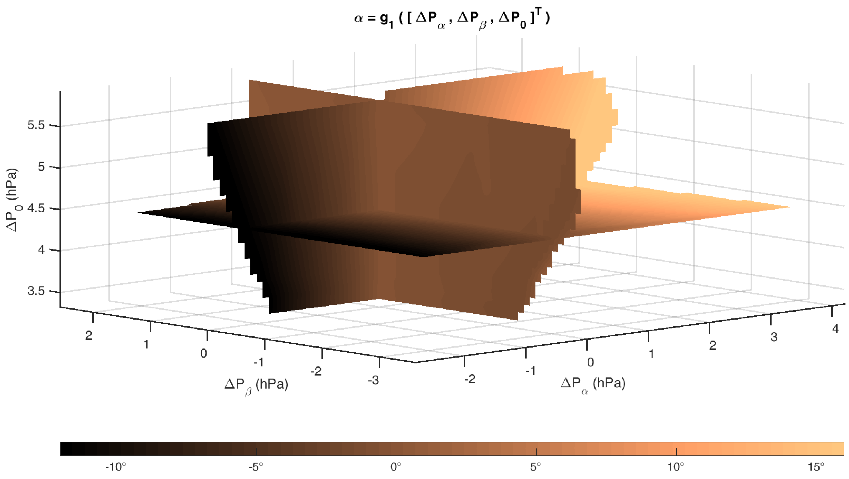
can be interpolated directly. Maximal sensitivity of this interpolation can be obtained by the gradient in each of the three directions. Thus, the maximum gradient is a representative of the maximum amplification of differential pressure measurements. The mentioned subset volume (represented by slices) to determine
is shown in
Figure 8 as one given example. It shows the dependency of the resulting angle of attack
on measured pressure differences
,
and
.
4.4.4. Validation of Wind Vectors Retrieved
The measurement strategy implicated square patterns to validate wind determination. An example of such a pattern and its retrieved wind vectors in the horizontal plane is shown in
Figure 9. Measurements during turns are excluded as the rotating flow field around the UAS does influence the calibration significantly compared to straight flight. In addition, the flight state in turn has a significant impact on the pressure field of the MHP; this effect cannot be addressed by a calibration in a wind-tunnel. Further, the retrieval of correct flight attitude out of INS/GNSS data may be subject to large errors during high dynamic maneuvers, as the navigation filter calculating the data fusion is attenuated. In [
46], it can be seen that attitude angle deviations between an INS/GNSS system of the same type as used in ALADINA compared to a reference system increase when motion changes from low dynamic to high dynamic. In addition, it is stated in [
46] that significantly varying sideslip angles will lead to deviations in roll. This is caused by the algorithm assumption, that there is no lateral velocity with respect to flight track.
Recent data analysis showed that the bottle-neck for wind uncertainty is the accuracy of the IMU [
24]. With a more precise and accurate IMU than the current MEMS-IMU (microelectromechanical systems-inertial measurement unit) in addition with more advanced strapdown calculation, wind determination would be improved noticeably.
4.4.5. Validation of Turbulence Measurements
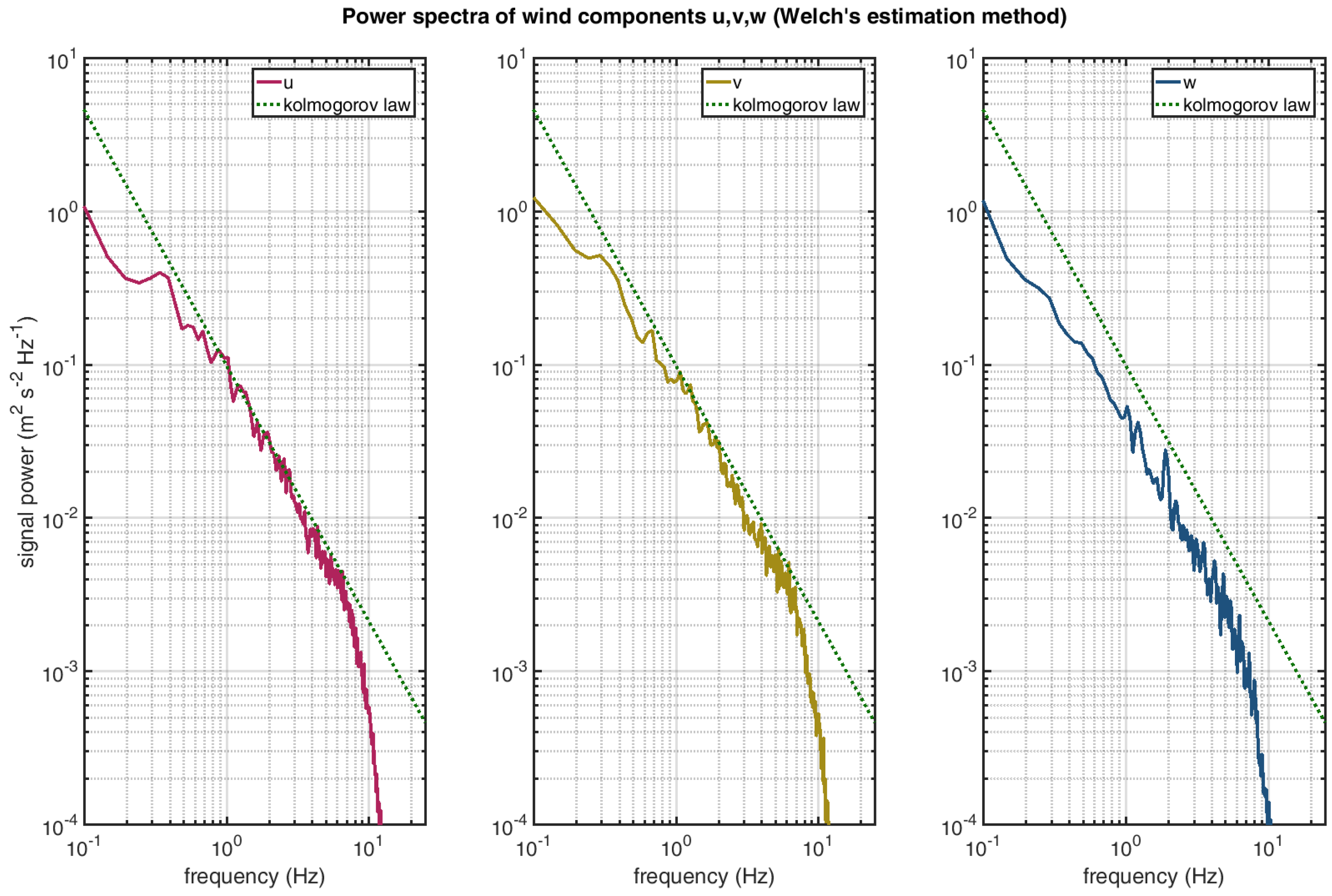
The ability to measure turbulence data is often shown by a spectral roll-off of calculated wind components.
Figure 10 shows the power spectra of the determined wind components. The power spectra were calculated using the method of Welch [
43] over three flights with a total data length of 1650 s. Data fit well to the
power law up to 7 Hz. At higher frequencies, the low-pass filter used for wind calculations attenuates the signal. In the data processing of the pressure sensors used, the authors use at least 10-times oversampling to ensure that amplitude and frequency information is not corrupted by aliasing filter effects.
4.5. Aerosol Characterization and Black Carbon Measurements
4.5.1. Sensors Installed
As presented in Altstädter et al. [
26] and Platis et al. [
21], ALADINA carries two condensation particles counters (CPCs, Model 3007, TSI Inc., St. Paul, MN, USA) and one optical particle counter (OPC, Model GT-526, Met One Instruments Inc., Washington, DC, USA) in order to classify the total aerosol particle number concentration and size distribution from ultra-fine particles up to particles belonging to the accumulation mode. The inlet is installed at the nose of ALADINA, close to the meteorological instrumentation. Two condensation particle counters of the same type with different threshold diameters are used as indicators for the total aerosol number concentration of freshly-formed particles. The hand-held instruments were miniaturized, tested and calibrated by the project partners of the Leibniz Institute for Tropospheric Research (TROPOS) in Leipzig, Germany. The lowest cut-off sizes were set during the last operation of 7 nm (
) and 12 nm (N
), respectively, by a fast resolution of 1.3 s. The OPC operates within six channels from 0.39
m–10
m in the particle diameter.
In addition, an aethalometer of the type MicroAeth® Model AE51 (AethLabs, San Francisco, CA, USA) has been installed in ALADINA to measure the BC (black carbon) mass concentration in the range of 0–1 mg m with a given resolution of 1 ng m. As the instrument is sensitive to vibrations, readings have to be low-pass filtered during post-processing. The accuracy was estimated as ±0.2 g m.
4.5.2. Validation of Aerosol Concentration and BC Measurements
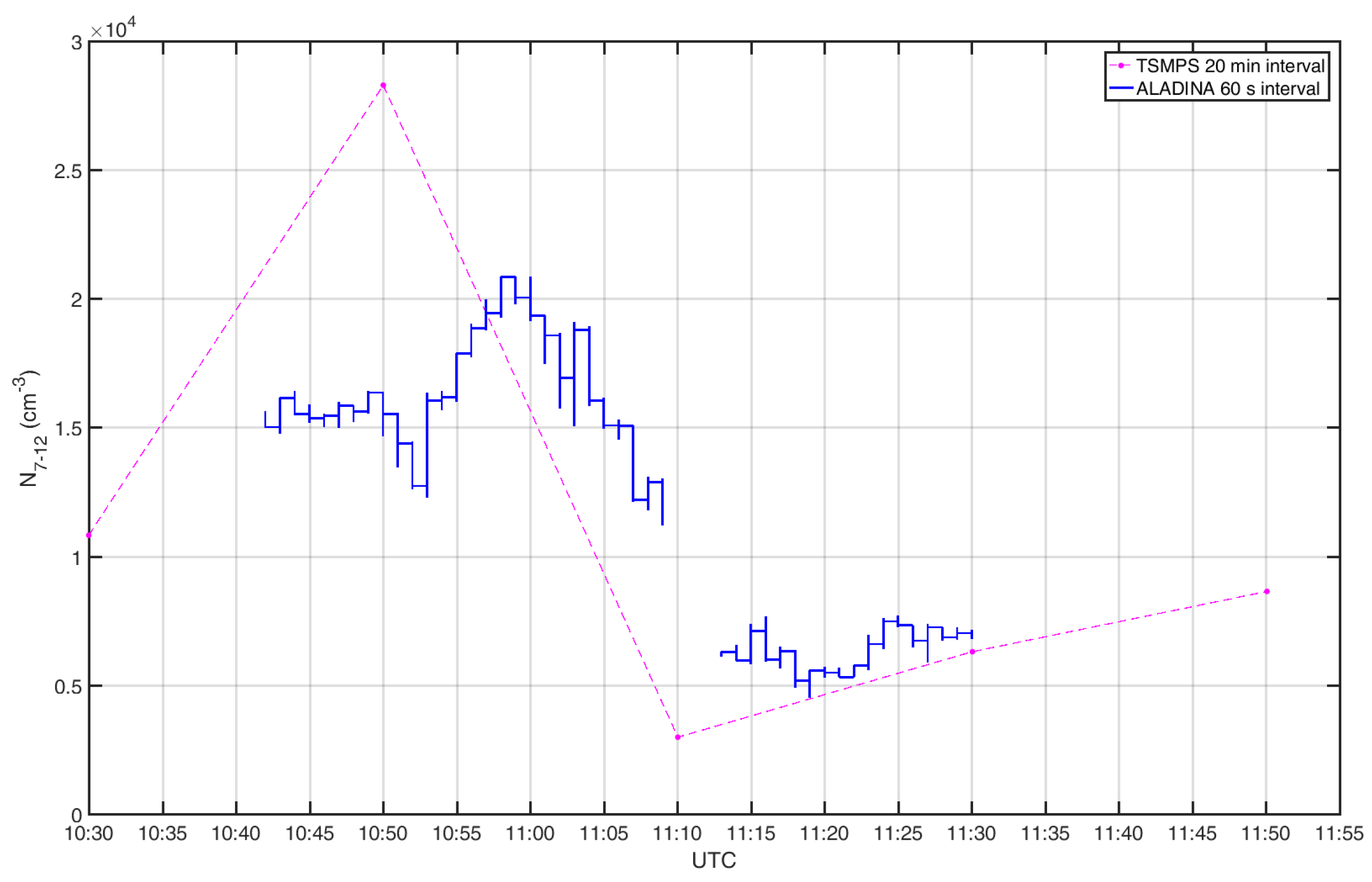
In order to show the reliability of the system to measure new particle formation,
Figure 11 is displayed. The total aerosol particle number concentration in the particle diameter between 7 and 12
m (
) measured by ALADINA is compared with a ground-based instrument (Twin Scan Mobility Particle Sizer (TSMPS) [
47]) that was mounted at the same time during a field study in Melpitz, Germany. During the time period from 10:30–11:55 UTC, four scanning intervals were performed with TSMPS (20 min average) and two measurement episodes with ALADINA from 10:41–11:09 UTC and between 11:12 and 11:30 UTC (1-min interval). During the measurement period, new particle formation occurred and can be seen in the enhanced total aerosol particle number concentration in the small diameter size between 7 and 12 nm. The total maximum of
= 2.8 ×10
was taken from the TSMPS at 10:50 UTC. The shapes are consistent; however, the CPCs underestimated the peak given by the difference on average. In total, the uncertainties are within 20%, as stated earlier from laboratory characterization.
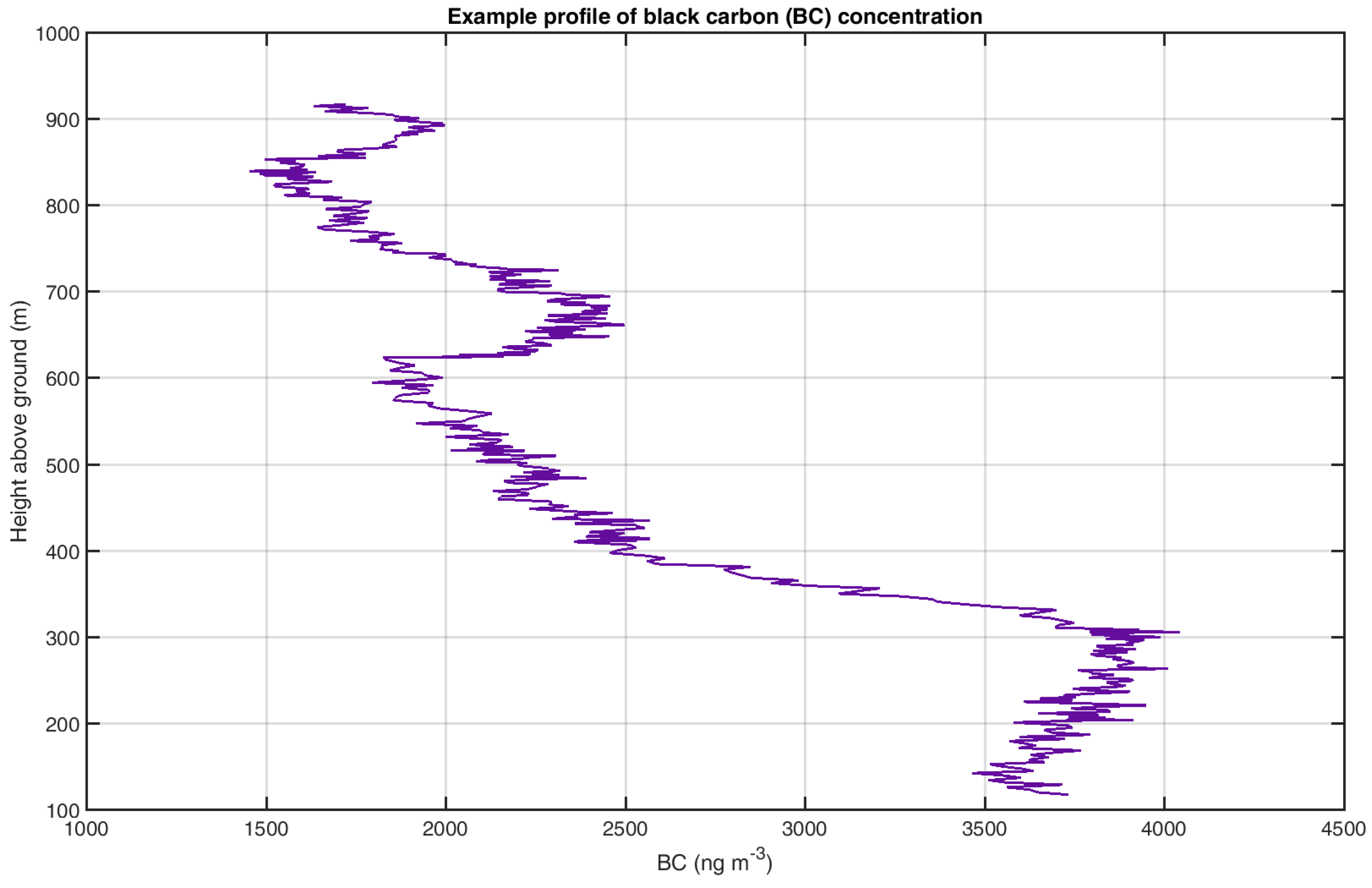
Figure 12 shows an example of the significant vertical variability of BC mass concentration, measured during the field campaign in Savè (Collines, Benin) of the DACCIWA project [
27]. BC mass concentrations are increasing to a total maximum of 4000 ng m
between the height of 100 and 300 m. Above and up to the height of 600 m, a significant decline of BC mass concentrations was observed. However, a second enhanced load was measured between the height of 610 and 800 m. The overall investigation was that enhanced BC loads were connected to nocturnal low-level jets and affected by low-level clouds. Further, BC studies influenced by different atmospheric boundary layer properties are still in process. Therefore, the intrinsic validation of BC mass concentration measurements through this likely possible profile is still weak.
During the field experiment in West Africa, harsh environmental conditions (dust, moisture of more than 90% RH, air temperatures higher than 40 °C) showed strong influences on the reliability of the aerosol instrumentation, so that in future perspectives, the sensor package will be insulated in a properly-defined environment.
4.6. Up- and Down-Welling Irradiance
4.6.1. Pyranometer for Estimating Solar Radiation
In addition to the meteorological and aerosol sensor package, silicium-based pyranometers of the type ML-01 (EKO Instruments, Tokyo, Japan) were installed on the UAS ALADINA: one downward looking and one upward looking with respect to the body-fixed coordinates. The pyranometers show the strong influence of sun incident angle (cf. datasheet) following a cosine law. The pyranometers are mainly used to identify if clouds were present, which is of importance for the interpretation of ABL conditions and aerosol properties. To retrieve shortwave downwelling irradiance, it is possible to calculate the sun incident angle on the sensor and provide a suitable estimation of irradiance values by assuming the cosine law. Since the sun is the only major directional irradiance source in clear sky, restoration of the pyranometer is more complicated on cloudy days. Partly sampled soil and scattering on aerosol particles could also be taken into account, despite their comparably low impact on the sensors.
4.6.2. Basic Correction of Sun Incident Angles on the Pyranometers
Irradiance measurements can be corrected by the angle of incidence
between the pyranometer normal axis and a vector pointing from the Sun to the pyranometers. Using such a correction, attenuated measured irradiance
caused by UAS attitude movements can be recovered to a corrected irradiance
in the direction of the Sun assuming clear skies. The correction applied follows the cosine law for a simple point source of irradiance (Sun on clear skies):
in addition to a factory calibration curve. The influence of incident angle errors increases with higher incident angles with respect to the sensor axis. The aim of the sun angle of incidence and attitude correction is a transformation of this measurement to an Earth-fixed coordinate system. With another trigonometric transformation using the solar zenith angle
, the shortwave downwelling irradiance:
can now be computed out of
.
4.6.3. Validation of Basic Irradiance Correction
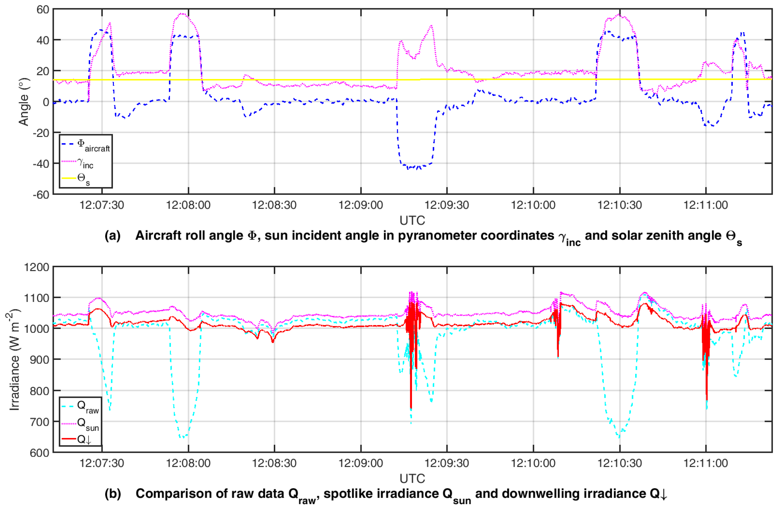
Figure 13 shows the influence of aircraft attitude in pyranometer readings and its correction through the cosine law over the incident angle of the sun with respect to the sensor axis.
Figure 13a shows the associated aircraft roll angles, the sun incident angles on the pyranometer sensor axis and the solar zenith angle. The correction of this influence was possible, since this example of measurements took place under almost clear skies. The data were obtained in Savè (Collines, Benin) during the campaign DACCIWA [
27] on 11 July 2016. In
Figure 13b. one can see a correction of approximately 400 Wm
. Residual correction errors are mainly caused by degraded attitude measurements during dynamic maneuvers (cf.
Section 4.4.4), but the tendency shows that the correlation between irradiance and aircraft attitude (mainly roll angle) can be reduced. Detailed sensor characteristics mentioned in the sensor datasheet were verified by laboratory tests. Secondary sources of errors could be partly sampled soil and scattering on aerosol particles.
4.7. Overview of the Sensor Package for Measuring ABL Properties
The sensors used on ALADINA are listed in
Table 2. Values for response time and accuracy are taken from the manuals of the manufacturers, calibrations and calculations presented in previous articles [
8,
10,
26,
32,
33].

 ,
, 


