Changes in Summer Pressure Patterns across the Late 1960s and Their Influence on Temperature Trends on the Eastern Coast of the Iberian Peninsula

Abstract

During the second half of the 20th century, in the littoral and pre-littoral areas of the Valencia region, the diurnal temperature range (DTR) registered a significant drop in summer (July and August). Meanwhile, in the same period in the lower Ebro Valley (Ebro Observatory), to the north of the Valencia region, the maximum temperature and DTR increased steeply. In order to explain the DTR drop in the coastal areas of the Valencia region, some studies have proposed an increase in the summer sea-surface temperature (SST) and others have attributed it to the urban heat island effect. Nevertheless, this drop occurred well before the current climate change was evident and therefore, before the rise of the SST. Furthermore, regarding the second proposed explanation, the drop in the DTR does not disappear when working with selected stations away from heavily urbanized areas. In this work, we propose that both the DTR rise at the Ebro Observatory and the DTR drop in the Valencia region are linked to the same process: changes in atmospheric circulation on a synoptic-scale in the North Atlantic that occurred in the late 1960s.

1. Introduction

The 20th century saw a worldwide rise in temperature of 0.89 °C [1] but this increase was not a uniform one all around the globe, neither spatially nor seasonally [2,3]. Actually, this increase was not a progressive one either and was, in fact, produced during two different phases. The first one lasted from 1910 to 1945 [4], while the second—and much more significant—phase has lasted from 1976 onward. From 1950 to the 1970s, a slightly negative trend was recorded. On the other hand, minimum temperatures increased at a faster rate than maximum temperatures during the latter half of the 20th century resulting in a significant decrease in the DTR (diurnal temperature range) for this period [5]. Furthermore, this widespread decrease in the DTR was only evident from 1950–1980 [6]; that is to say, maximum and minimum temperatures have increased roughly at the same rate from the beginning of the current period of global warming.

There are many studies which indicate that the temperature evolution in the Iberian Peninsula (IP) is analogous to the evolution of temperatures worldwide. For example, Brunet et al. [2] detected two periods of rising temperature (1901–1949 and from 1973 onward) and another period with a fall (1950–1972). In Spain, the most remarkable feature of the twentieth century was an abrupt and strong warming recorded from the early 1970s onward [7,8,9,10]. Furthermore, the results of the majority of studies regarding changes in Spanish temperatures during the 20th century show that maximum temperatures (Tx) increased at greater rates than minimum temperatures (Tn) both over the whole mainland [11,12] and over several sub-regions [13,14,15,16]. During the period 1901–2005, Tx have increased by twice as much as Tn [2] on average. However, this long-term asymmetry between maximum and minimum temperatures was clearly broken in the period 1973–2005 [2]—a result which is in agreement with the corresponding worldwide temperature behaviour for that period [6].

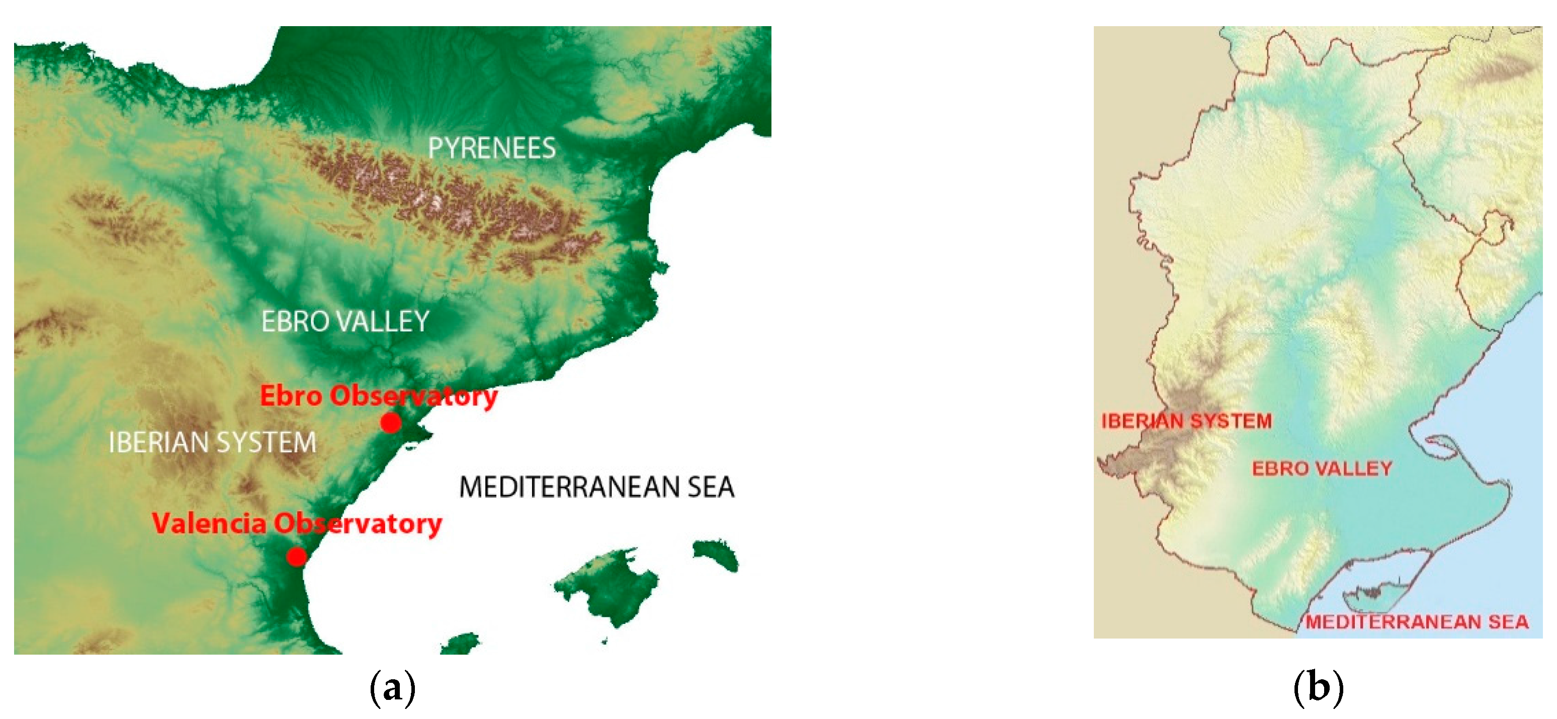
In the Valencia region (the eastern-central part of the IP, on the Mediterranean coast) Miró and Estrela [17,18], found a much more significant increase in minimum summer temperatures (July and August) compared to the increase in maximum temperatures at the coastal and pre-coastal observatories in the period 1958–2003. In their study, the authors only selected stations away from heavily urbanized areas in order to prevent the urban heat island effect. Moreover, at the inland stations, the trends of maximum and minimum temperatures evolved in a similar way. They found a stronger increase of maximum temperatures at the inland stations when compared to the increase seen at those on the coast and a notable SST (sea-surface temperature) increase in August which can be reflected in the stronger increment of temperature in August in comparison with July. The combination of this warmer sea with a greater predominance of tropical air masses has been discussed by the authors as the causes of the drop observed in the thermal oscillation in the coastal areas. However, that explanation is not entirely consistent with the fact that the main DTR drop in the littoral and pre-littoral areas occurred before 1980 (Figures 11 and 12 in Miró and Estrela [18]) well before the current period of climate change became evident. In fact, the DTR drop recorded from 1980 onwards is very small in July and negligible in August.

On the other hand, Quereda et al. [19] related the differential behaviour of Tx in comparison with Tn (i.e., the fall in DTR) seen at the main observatories of the coastal area of the Valencia region in the second half of the 20th century to urbanization because this asymmetry has not been found in the respective trends of the rural observatories’ time series. Furthermore, Quereda et al. [20] estimated that the magnitude of the urban heat island effect could account for between 70% and 80% of the recorded warming trend in Western Mediterranean cities.

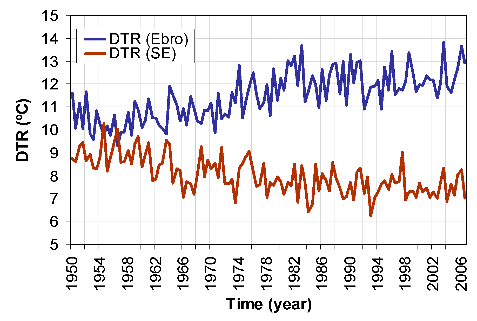
Moreover, while the DTR fell in the coastal area of the Valencia region, at the same time the DTR rose quickly at the Ebro Observatory, only a few hundred kilometres to the north. We believe that, despite the fact that the effects of urbanization on the negative trends of the DTR in the central and southern part of the Mediterranean area of the IP may be significant, this differential evolution of Tx trends in comparison with Tn trends is also related to the strong positive trend of the DTR recorded at the Ebro Observatory. Both asymmetric DTR trends can be partly explained by a different reaction—on a regional level—to changes in atmospheric circulation on a synoptic-scale in the North Atlantic.

There are various factors which can contribute to temperatures recorded in different regions evolving differently. Favà et al. [21] found a differential behaviour of Tx trends in the NW IP (positive) compared to those in the SE IP (negative) in the months of summer (July and August), which was related to the strong increase in the SNAO recorded at the end of the 1960s [22]. The SNAO is the first EOF obtained from a matrix of covariances of the North Atlantic sea level pressure anomalies [23]. The SNAO index is strongly linked to temperatures and precipitation in the north and west of Europe although its influence on southeast Europe is slightly lower and in the opposite sense. In the IP, the correlation between SNAO and precipitation is of positive sign (with the exception of the NW), as in SE Europe, Italy and the Balkans [24].

The main goal of this work is to determine, from the atmospheric circulation, the principal synoptic structures related to the increase in the Tx and DTR in the Ebro Observatory region in comparison with the same variables further south. With this aim in mind, after identifying these structures, we studied whether possible changes in their frequency can help to explain the differential behaviour of the Tx and DTR trends around the Ebro Observatory region in comparison with the east and southeast (SE) IP region.

The paper will be structured as follows. The data used and the proposed methodology are presented in Section 2. In this section, the relationship between the wind and the pressure gradient on a synoptic-scale at the Ebro Observatory is also studied to justify the sorting of data into ‘Northern days’ and ‘Southern days.’ In Section 3 we study the relationship between the relative vorticity at sea level and maximum temperatures at the Valencia Observatory. In Section 4 we propose an index based on the atmospheric circulation related to the difference between the maximum temperatures recorded at the Ebro Observatory and those of the Valencia Observatory. The results are presented in Section 5 and finally we present the discussion and conclusions.

2. Data and Methodology

2.1. Data

The following daily data were used to carry out this study:

• Data from the NCEP/NCAR (National Centres for Environmental Prediction/National Centre for Atmospheric Research [25] for a latitude-longitude resolution of 2.5° × 2.5°—specifically the mean sea level pressure (MSLP), the 500 hPa geopotential height (Z500) and the Z500–Z1000 thickness for the period 1948–2006.
• Data from the Agencia Estatal de Meteorología (AEMET—Spanish Meteorology Agency) of maximum and minimum daily temperatures at Valencia and Ebro Observatory (1948–2006) needed for a first PCA analysis.
• Daily maximum temperature data from the Spain02 dataset (1950–2007) [26].
• Wind speed and direction data from AEMET of the Ebro Observatory (1948–2006) and Valencia Observatory (1997–2011).
• Data from the Servei Meteorològic de Catalunya (Catalan Meteorological Service) (1996–2006).

We have chosen the Ebro and Valencia Observatories (Figure 1) for a first analysis as they are reference observatories for AEMET because of their good quality, comprehensive and reliable data. Both are located on the eastern coast of the IP; Valencia in the central part and Ebro about 200 km to the north. The Ebro observatory is a centennial one and atmospheric weather variables have been regularly measured there ever since its foundation [27].

2.2. Methodology

To determine the trends’ significance, we used a Monte Carlo test, following the same methodology as Turco and Llasat [28]. To compute each Bootstrap distribution, we carried out 1000 iterations. We divided the data into two groups of days according to the sign of the meridional component of the wind at ground level at the point (42.5° N, 0° E)—just over the Pyrenees [21,29]. When this component is southward (58% of the days, ‘Northern days’), the northern IP is, on average, under the influence of a northern air influx linked to the NE edge of the Azores High. On the other hand, when the meridional component of the flow is northward (42% of the days, ‘Southern days’), then the IP is in general more influenced by Mediterranean and African air masses.

In this paper, we focus on the Northern days because, as we shall see, it is during these days when the reasons for the differential behaviour in the Tx along the eastern coast of the IP becomes more evident. In this set of days, due to the orography of the area, the continental conditions in the Ebro Observatory region are in general enhanced. When the westward component of the pressure gradient in the Pyrenees is positive, the anticyclone is in the west. Then it is to be expected that the flow will have a northern component and, due to friction and the orographical effect of the Pyrenees, the flow at the Ebro Observatory will have a positive westerly component (to the sea) and when the offshore component of the synoptic wind is positive, a stronger onshore temperature gradient is needed to develop a sea breeze [30]. The Ebro Observatory is located in the pre-littoral area and that is the reason why any variation in the spatial scope of the sea breeze is well reflected in its maximum temperatures. In general, the opposite happens during the Southern days, when the sea breeze is enhanced, which is why the DTR of the Northern days has significantly higher values with respect to Southern days. Valencia observatory is located on the coast and, therefore, the influence of sea air on its temperatures is much greater and for the sea breeze to be cancelled, the westward pressure gradient must be stronger.

3. The Relative Vorticity at Sea Level and the Temperature at Valencia Observatory

After investigating which variables of the atmospheric circulation field may give us more information about the difference we can expect to find at a specific moment between the Tx and DTR anomalies of the areas around the Ebro Observatory and Valencia Observatory, we found that the relative vorticity at sea level plays a significant role in the sense that it allows us to describe easily how the surface pressure gradients will be distributed along the eastern IP coast. These pressure gradients are determining factors to shift the balance for the regional conditions of both observatories towards continental air or marine air (the Valencia one is located on the coast, while the Ebro Observatory is on the pre-coast—a little inland).

We calculated the relative vorticity (ζ) at each grid point in the window (30° W–30° E, 25° N–60° N) by firstly computing the approximate components of the theoretical geostrophic wind at sea level (u, v), setting out from the sea level pressure gradient ($\nabla p$), the Coriolis parameter (ƒ = 2Ω·sinØ, where Ω is the angular speed of rotation of the earth and Ø is the latitude) and the sea level air density (ρ) [31]:

$$u\approx -\frac{1}{\rho ·f}\frac{\partial p}{\partial y};v\approx \frac{1}{\rho ·f}\frac{\partial p}{\partial x};\zeta =\frac{\partial v}{\partial x}-\frac{\partial u}{\partial y}$$

(1)

We found that both the Tx and the DTR at both observatories—but especially at Valencia—can be related with the way the relative vorticity is distributed at sea level. At Valencia Observatory, owing to its geographical location, the (marine/continental) wind direction has a direct relation with the Tx and DTR; on average, the westerly wind due to its run over the inland IP, is warmer than the wind from the east (which has followed a marine route). At the Ebro Observatory, this relationship becomes more complex, though, partly due to the orographic conditions.

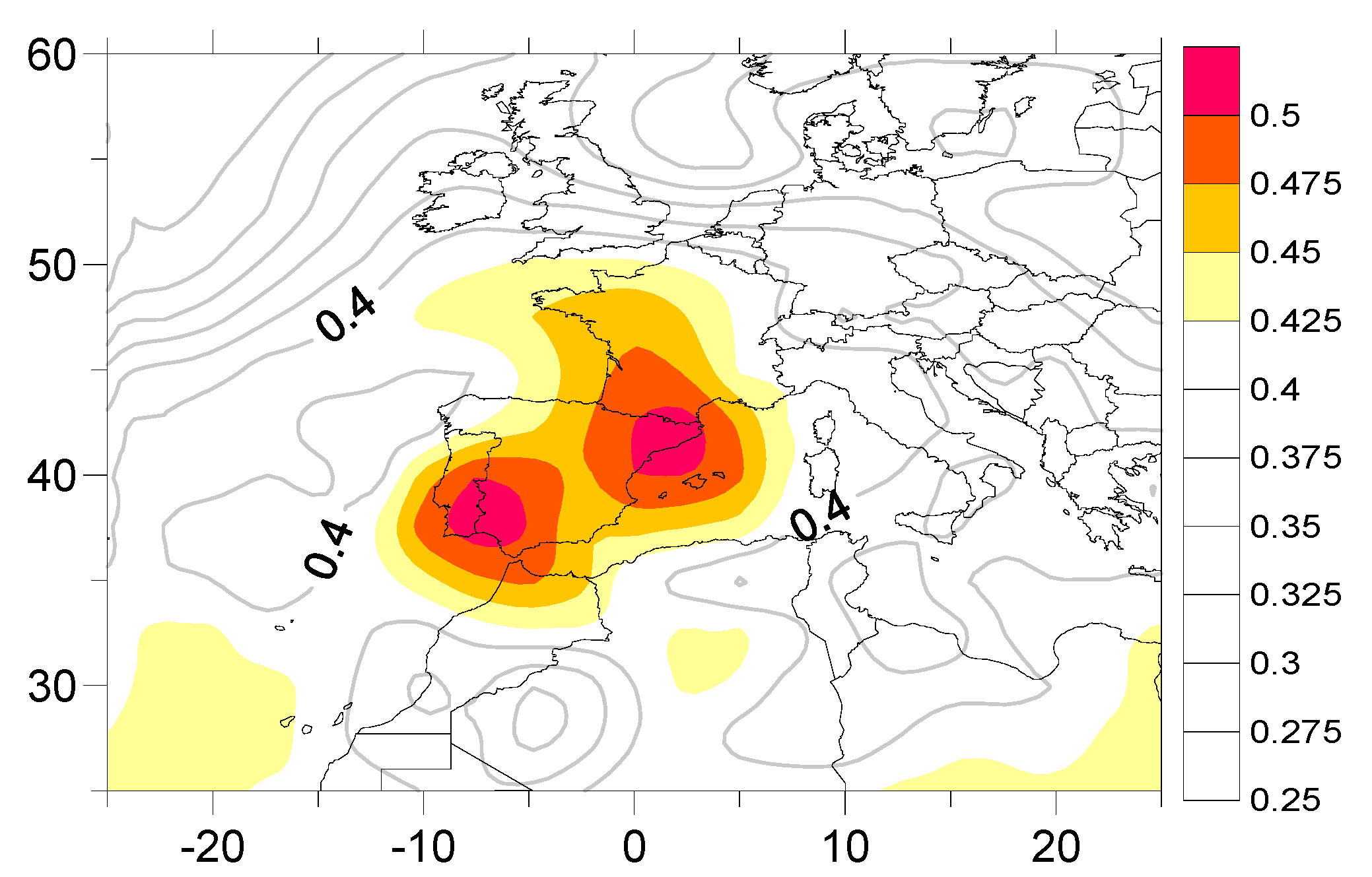
We studied how the differences between the relative vorticity of any random pair of points and the time series of Tx at the Valencia Observatory (TxValencia) correlate. The map in Figure 2 shows the spatial distribution of the maximum values of the former correlations and indicates that the pair of points for which the difference between their relative vorticity values correlate as closely as possible with TxValencia are (7.5° W, 37.5° N) and (2.5° E, 42.5° N). To draw up this map we looked at all the points, searching for the maximum possible absolute value of the correlation between the relative vorticity difference at each point with respect to any other point and the TxValencia time series. First, we calculated the sea level relative vorticity at each point; then we combined the first point with all the others in order to obtain a matrix of values corresponding to the difference of relative vorticity between the first point and all the others. Then we computed another matrix from the absolute value of the correlations between the elements of the former matrix and TxValencia. Finally, we selected from that matrix the maximum absolute value, which is the value plotted in Figure 2 corresponding to the first point. This procedure was applied to all the other points.

This map shows very high values for the correlations at most points—which is not surprising given that for any specific point it is likely that we can find another one where, when subtracting their relative vorticities, we can relate the value obtained from the subtraction with TxValencia merely by chance. However, the areas of maximum correlation have to be paired between themselves in the sense that only the points in these zones have been used to obtain such high correlation values. In these cases, the high correlation values cannot be obtained by chance due to their convergence to two well-defined spatial regions (NE IP and SW IP). There must be a physical explanation for this spatial convergence that we shall look at later.

We called the relative vorticity of the point with maximum correlation in the NE (2.5° E, 42.5° N) ‘VortNE’ and the corresponding relative vorticity in the SW (7.5° W, 37.5° N) ‘VortSW’ (the centres of the red-coloured regions of the map of Figure 2).

Wind direction is measured in degrees clockwise from the geographical north as seen in

Table 1. Wind Direction.

Wind Direction	N	E	S	W
Angle	0°	90°	180°	270°

. The wind direction of the first quadrant is between 0° and 90°, the second quadrant wind is between 90° and 180° and so on until the fourth quadrant.

4. Calculating the Synoptic Patterns Related to a Maximum Differentiation between Tx and DTR in the Ebro and Valencia Regions

Although the former relative vorticities (VortSW and VortNE) are more related to Valencia Tx than Ebro Tx, they could play a part in explaining the differential behaviour between both observatories. However, owing to their proximity, it is quite probable that most of the synoptic situations generate patterns of Tx anomalies with the same sign in both regions. For example, a warm advection centred in the eastern IP will make Tx rise all along the coast. The signal we are searching for will probably be hidden behind the kind of weather common to both areas.

To obtain the synoptic patterns we are searching for, we used a Principal Components Analysis (PCA) with the following daily variables for the period 1948–2006 corresponding to the Northern days, after eliminating the trend:

• The relative vorticities of the points with maximum correlation: VortNE and VortSW.
• Tx and DTR at Ebro and Valencia Observatories.
• Temperature at 850 hPa (T850) in the grid point closest to the Ebro Observatory and to Valencia Observatory (40° N, 0° E).

We used the NCAR Command Language [32] to compute the PCA. We included the T850 in the PCA to determine whether the anomalies obtained at both observatories have a relationship with the anomalies in temperatures at mid-levels on a synoptic scale or, on the contrary, if they are due to lower scale processes.

On the other hand, the summer IP Tx and DTR are positively correlated to the sunshine duration [33]. We found strong correlations specifically between DTR and sunshine duration at the Ebro and Valencia Observatories (r = 0.57, > 99% and r = 0.41, >99% respectively, with daily data in the period 1972–2006). However, we did not include the sunshine hours data in the set of variables selected for the PCA because we did not find any significant trend in the sunshine duration for the period 1954–1981 (when the differential behaviour of both Tx trends is at its maximum) at the Valencia Observatory and because the sunshine duration data at the Ebro Observatory is only available from 1972 onwards.

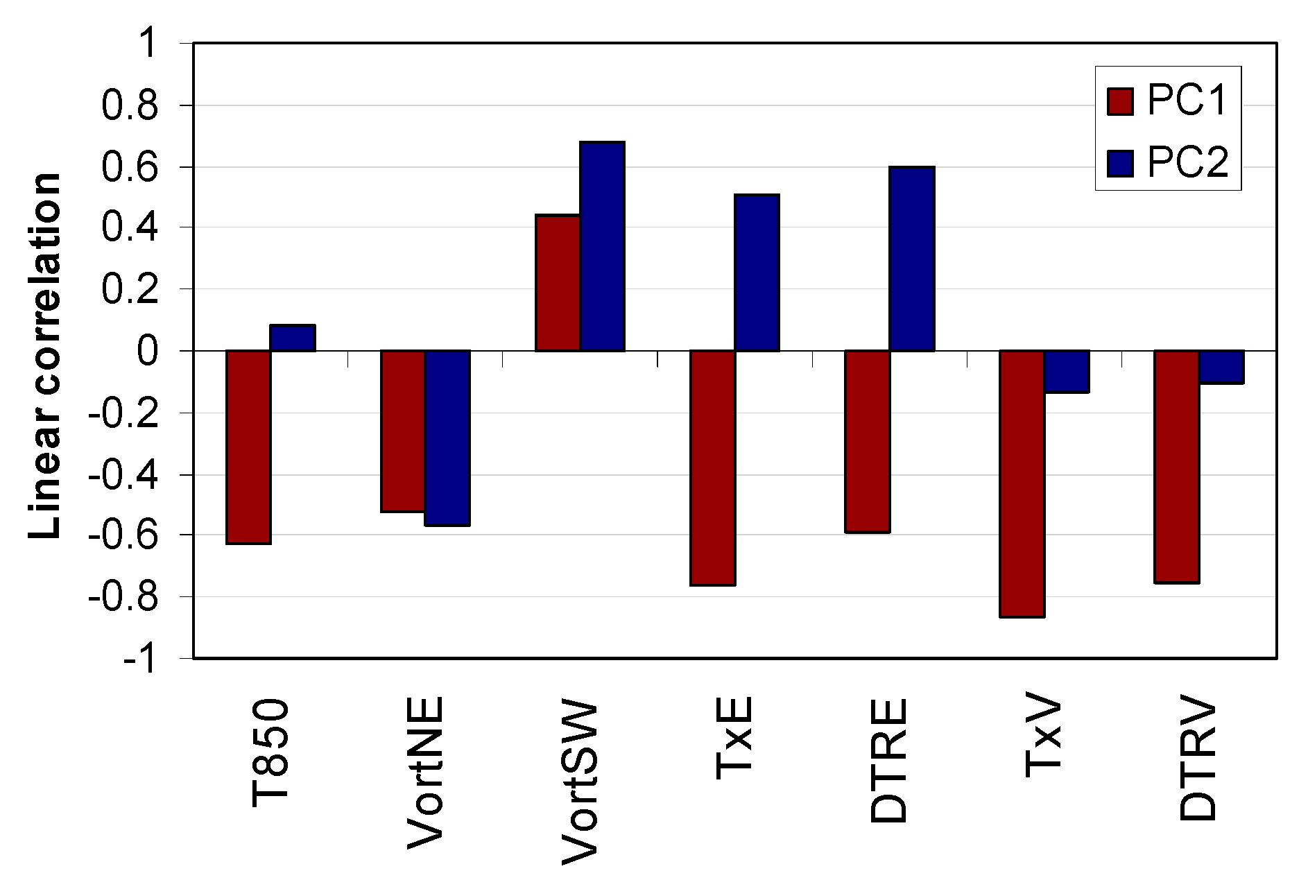
Figure 3 shows the correlations of the seven entry variables of the analysis with the first and the second principal components (PC1 and PC2, which account for 65% of the total variance of the set of the seven variables). This graph shows how the structure linked to PC1 corresponds to a weather pattern which generates a homogeneous behaviour at both observatories with respect to both the Tx anomalies and the DTR ones. Although the structure linked to PC1 explains the greater proportion of variation (44%), we focused on the structure linked to PC2 as it adjusts exactly to what we are searching for: changes in vorticities (VortNE, VortSW) linked to a considerable increase in the Tx and DTR at the Ebro Observatory and at the same time to a discrete drop in the Tx and DTR at the Valencia Observatory. Therefore, PC2 is related to a weather pattern linked to important deviations in Tx and DTR anomalies at both observatories. The correlation obtained between PC2 and the difference TxEbro–TxValencia is very significant (r = 0.72, >99%).

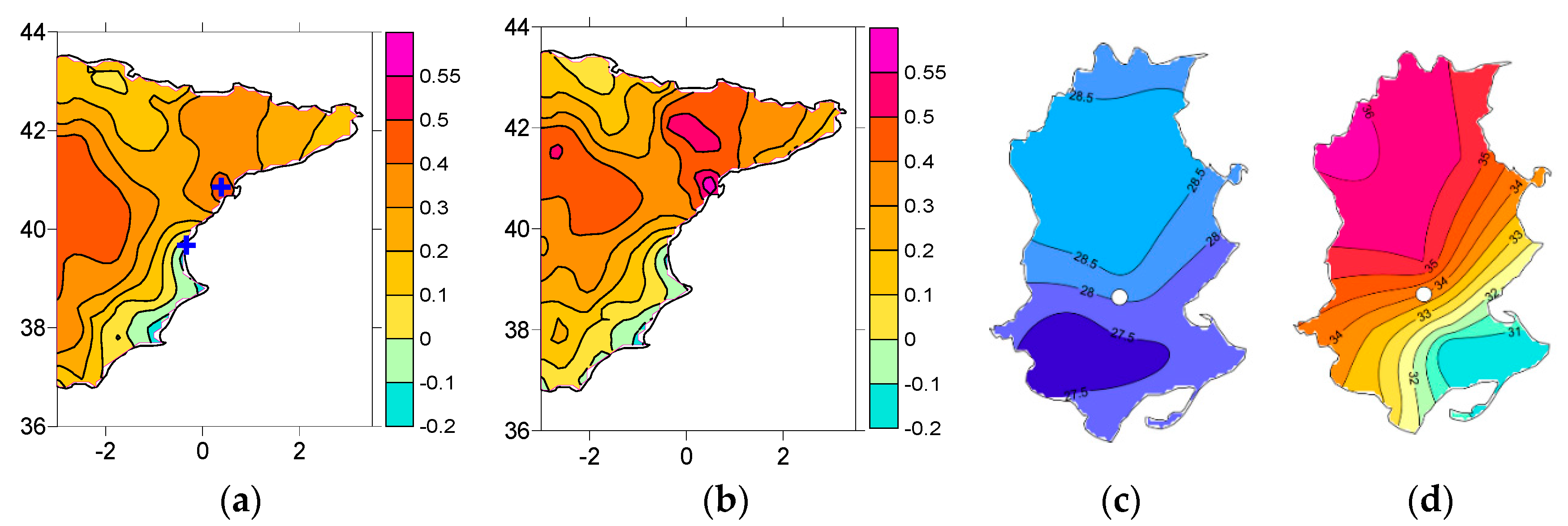
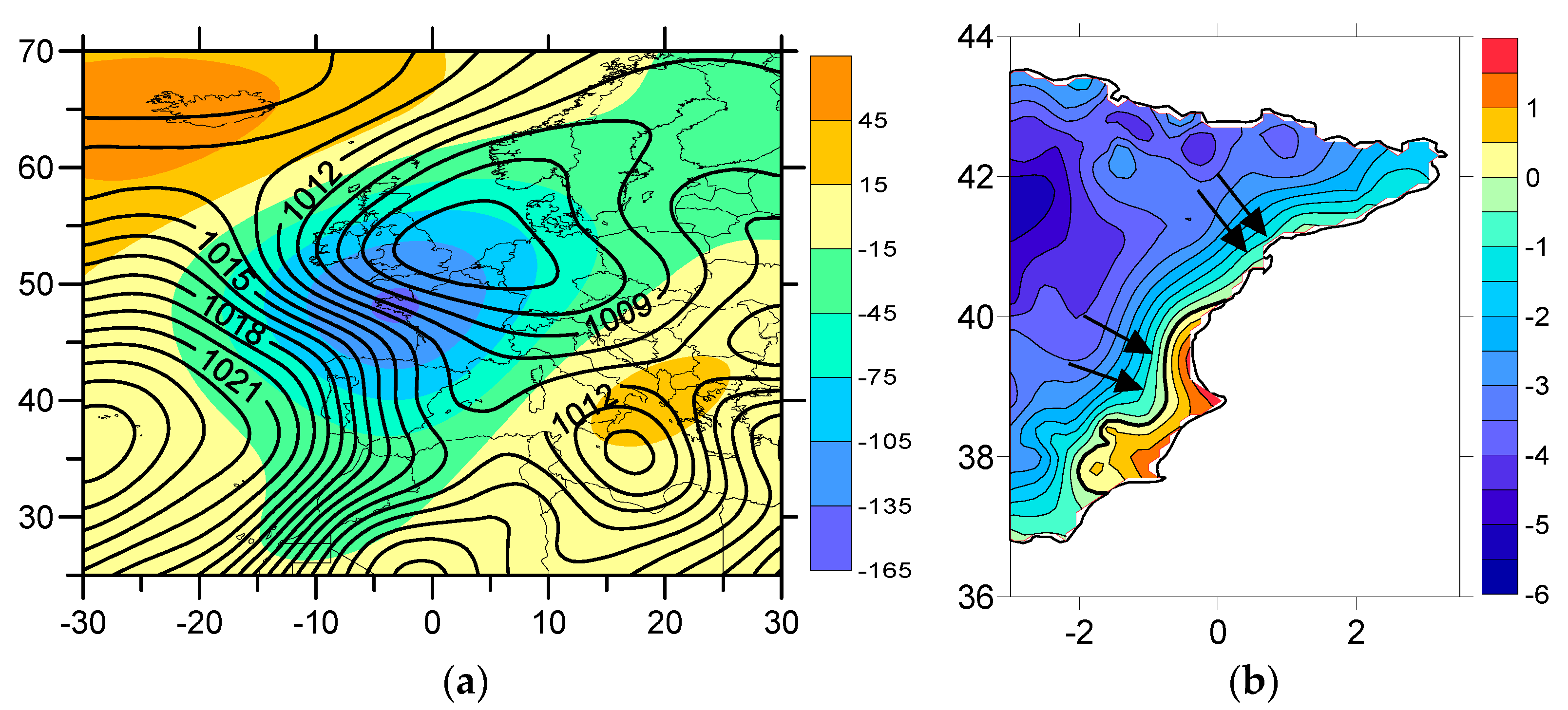
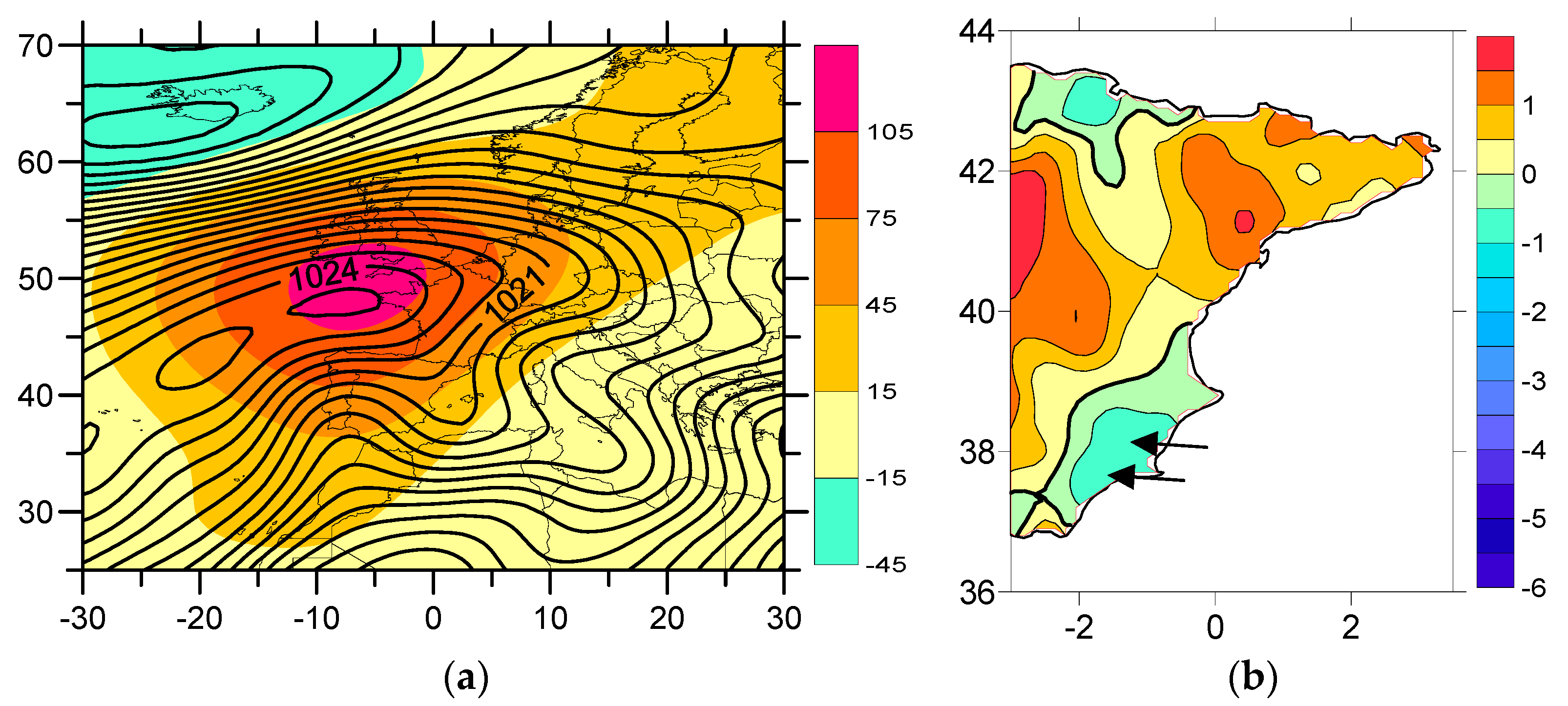
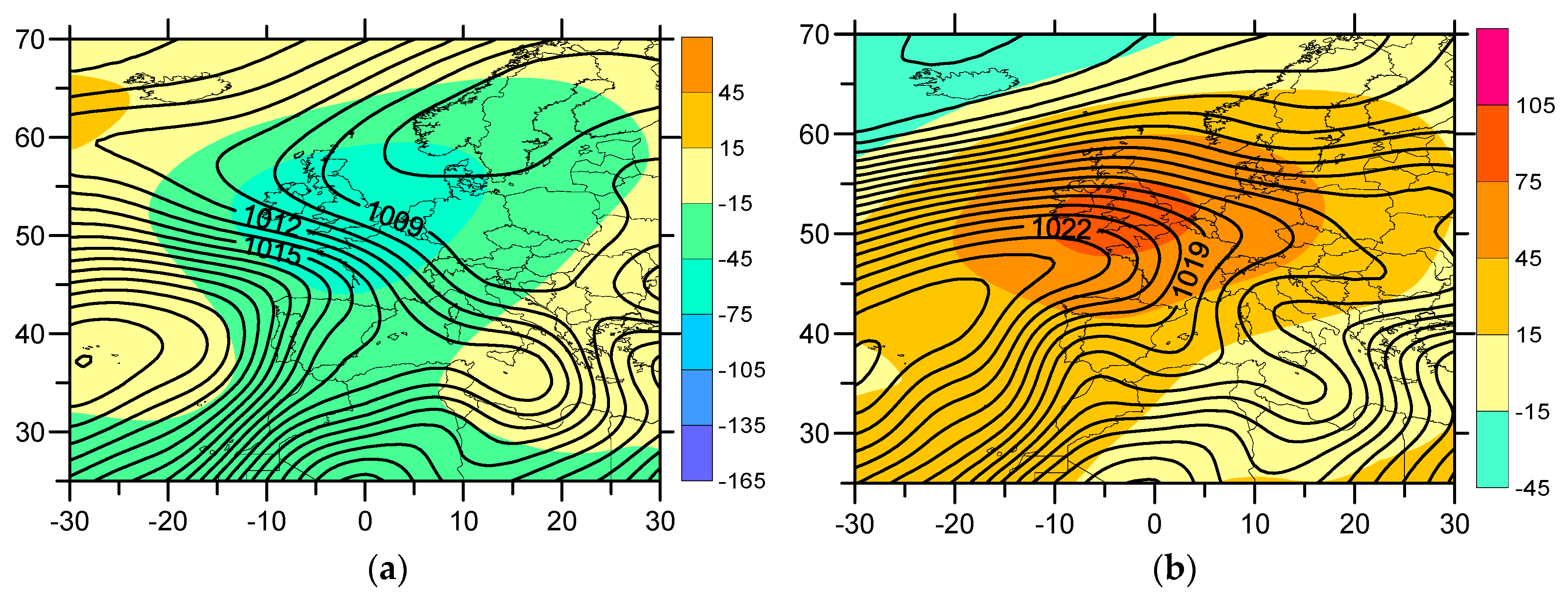
The correlation map of Figure 4a shows the spatial distribution of correlations between Tx and PC2 and the corresponding map of Figure 4b shows the correlations between DTR and PC2. On days when the PC2 reaches very negative values, the Tx of the lower Ebro Valley are low and there is a weak cross-shore temperature gradient (Figure 4c) owing to the homogenizing effect of the cold northerly wind which, as we shall see, is linked to the negative phase of the PC2. On the contrary, for high values of PC2, both the Tx and the towards-inland cross-shore temperature gradient experience much higher values (Figure 4d).

The result of this PCA shows structures which combine anomalies obtained directly from the observation in both regions with anomalies of variables of the atmospheric circulation field on a large scale and therefore these structures have to be seen on a synoptic-scale. On the other hand, an important difference to be pointed out between the two structures we find is that, in the case of the first one (EOF1), the Tx and DTR at both stations share the same behaviour and also have the same behaviour with respect to T850. This confirms that the positive (negative) anomalies are in this case due to a large scale synoptic situation associated with a warm (cool) advection and that this probably affects all the eastern IP area. In the case of the structure linked to PC2, though, the T850 does not show any correlation, which suggests that the Tx and DTR anomalies in this case are due to a process with a more regional scope.

Another important conclusion that can be inferred from the PCA is the fact that, while at the Ebro Observatory it is possible to find synoptic structures related to high absolute values of Tx and DTR regardless of the sign of the difference (VortNE-VortSW), this is not the case for the Valencia Observatory. In general, the main way to find significant positive (negative) anomalies of DTR and Tx at the Valencia Observatory is when the difference VortNE-VortSW is positive (negative). This is a result of the geographical location of Valencia: when VortNE-VortSW is positive, the direction of the wind to be expected is from the fourth quadrant, which is warmer than on average because of the air heating related to its crossing of the IP under high insolation conditions and to the adiabatic compression due to the loss of altitude. When VortNE-VortSW is negative, the opposite effect occurs: then the direction of the wind to be expected is from the second quadrant, which, in general, is cooler than on average as a result of the mild sea air. This is true not only for Valencia but for all the SE coast in general. This singularity of the Tx in the Valencia region with regard to the relative vorticity explains the correlations map of Figure 2.

Our aim is to study the time series of PC2 so as to evaluate its possible relationship with the differential behaviour of the Tx along the east IP coast. Also, we are interested in the time series of PC1, because it is the leading principal component and, hence, a large percentage of variance is linked to it. However, the time series of PC1 and PC2 contain direct information regarding the Tx and DTR of both stations (Ebro and Valencia) and it would not make sense to try to explain the increase of the Ebro DTR and the decrease of the Valencia DTR, from indices which already contain direct information about these variables. For this reason, we calculated two new indices (iPCN1 and iPCN2) from data which only come from the NCEP reanalysis: Z500, MSLP, Z500-Z1000 and sea level relative vorticity.

On the other hand, it is important that the new indices ‘inherit’ the links of the original indices with the PCA entry variables (Figure 3) (VortNE, VortSW, TxE, DTRE, TxV, DTRV); this way, the information obtained from the PCA will be preserved as much as possible. With the aim of achieving the maximum possible correlation between the new indices (iPCN1, iPCN2) and the original ones (PC1, PC2), we calculated the new indices by using the same procedure as Favà et al. [29].

The time series of these new two indices (iPCN1 and iPCN2) are computed exclusively from reanalysis and correspond to well-defined spatial structures. In order to compute the iPCN1 index, we selected the days with extreme values (higher than the 90th percentile) corresponding to the positive phase of PC1. Using this days, we then calculated the patterns of normalized anomalies corresponding to the fields of sea level pressure (MSLP), geopotential height 500 hPa (Z500), thickness (Z500–Z1000) and sea level relative vorticity in the window (30° W–30° E, 35° N–60° N). In this study, the relative vorticity field is needed because, as we have seen, it is closely related to the Tx and DTR at Valencia Observatory.

In order to calculate the normalized anomalies, for each field, we calculated the average value and standard deviation at every grid point (for the study period). Then we calculated the normalized daily anomalies for each point by subtracting the average value of the field at that point from the daily value of the field at that point (one per day) and dividing the result by the standard deviation at that point.

The four patterns of average anomalies corresponding to PC1 were obtained by selecting those days with PC1 values higher than the 90th percentile (n days) and calculating for this set of days, the average values of the anomalies at each point (p) for each of the four fields (Z500, Z500–Z1000 (thickness), MSLP and sea level relative vorticity):

$$\mathrm{Z}500\_\mathrm{P}\mathrm{C}1(p)=\frac{1}{n}{\displaystyle \sum _{t=1}^{t=n}\mathrm{Z}500\_(p,t)}thickness\_\mathrm{PC}1(p)=\frac{1}{n}{\displaystyle \sum _{t=1}^{t=n}thickness\_(p,t)}$$

(2)

$$\mathrm{M}\mathrm{S}\mathrm{L}\mathrm{P}\_\mathrm{P}\mathrm{C}1(p)=\frac{1}{n}{\displaystyle \sum _{t=1}^{t=n}\mathrm{M}\mathrm{S}\mathrm{L}\mathrm{P}\_(p,t)}vort\_\mathrm{PC}1(p)=\frac{1}{n}{\displaystyle \sum _{t=1}^{t=n}vort\_(p,t)}$$

(3)

We obtained the new index iPCN1 by projecting the four former patterns onto the normalized daily field anomalies of MSLP, Z500, Z500–Z1000 (thickness) and sea level relative vorticity in the window (30° W–30° E, 35° N–60° N) (corresponding to 275 grid points) and finally by adding the four obtained values.

$$\begin{array}{l}\mathrm{iPCN}1(\mathrm{t})={\displaystyle {\sum }_{p=1}^{p=275}\mathrm{Z}500(p,t)\times \mathrm{Z}500\_\mathrm{P}\mathrm{C}1(p)}+{\displaystyle {\sum }_{p=1}^{p=275}thickness(p,t)\times thickness\_\mathrm{P}\mathrm{C}1(p)}\\ +{\displaystyle {\sum }_{p=1}^{p=275}\mathrm{M}\mathrm{S}\mathrm{L}\mathrm{P}(p,t)\times \mathrm{M}\mathrm{S}\mathrm{L}\mathrm{P}\_\mathrm{P}\mathrm{C}1(p)}+{\displaystyle {\sum }_{p=1}^{p=275}2\times vort(p,t)\times vort\_\mathrm{P}\mathrm{C}1(p)}\end{array}$$

(4)

The ‘normalized daily field anomalies’ refers to the set of daily values of normalized anomalies corresponding to each of the four fields. For each field, there is a normalized anomaly for each grid point on each of the days of the selected period.

The index iPCN2 was calculated in the same way that iPCN1 but the four patterns of average anomalies corresponding to PC2 were obtained by selecting those days with PC2 values lower than the 10th percentile. We found the best correlations between PC1 and iPC1 and between PC2 and iPC2 projecting onto the normalized anomaly fields the cold phase of the two indices (PC1 and PC2), hence we selected the days with PC1 values higher than the 90th percentile (the cooler days in the IP) and the days with PC2 values lower than the 10th percentile (the cooler days in the IP). By giving more weight to the vorticity (doubling it), we were able to maximize the correlations between these new indices (iPCN1 and iPC2N) and the former ones (0.74 and 0.73 respectively).

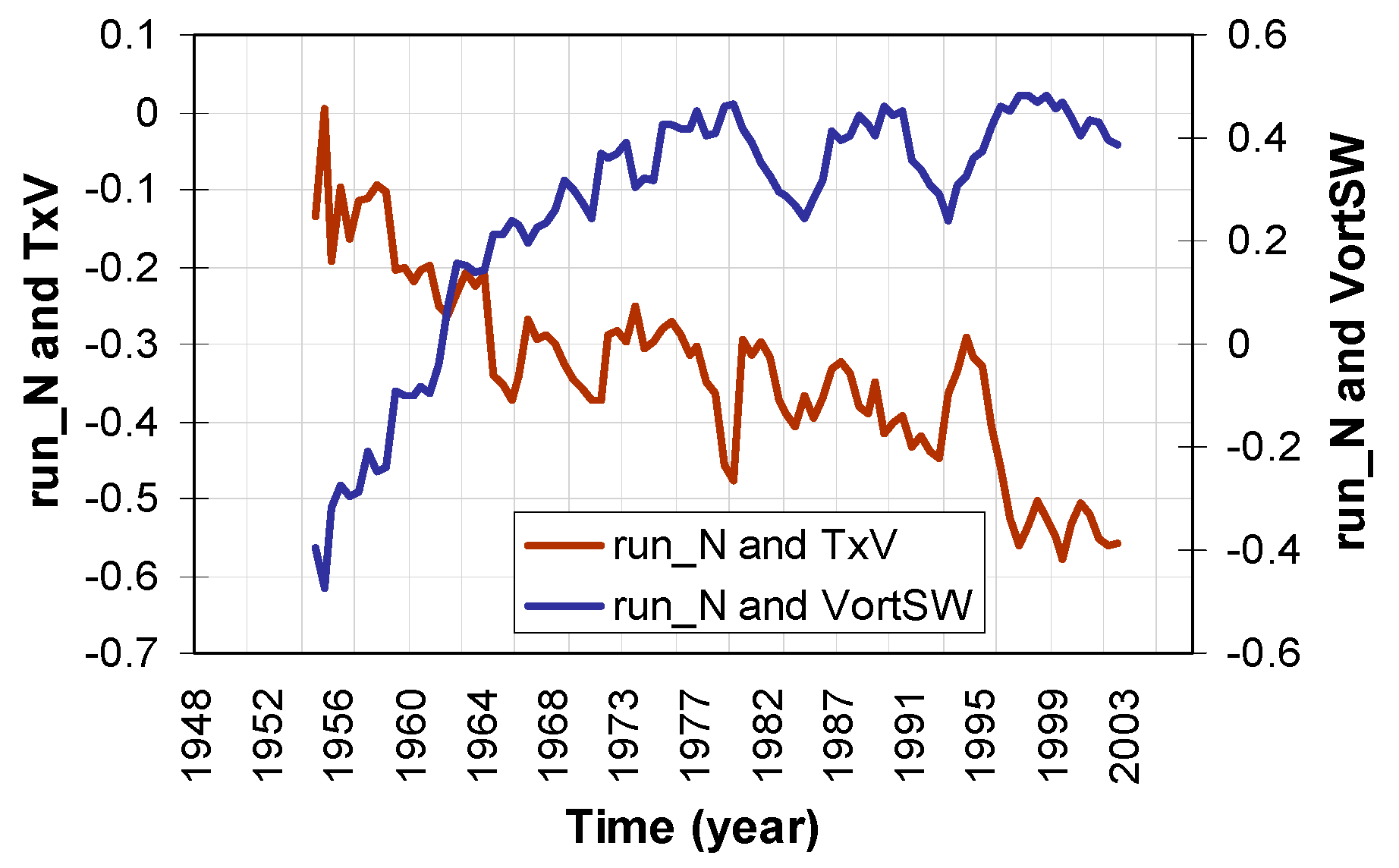
In order to check whether the links between the set of PCA entry variables and the new indices we calculated (iPCN1 and iPCN2) are preserved, we calculated the correlations between them and VortSW, VortNE, Tx, Tn and DTR at the Ebro and Valencia Observatories for the period 1948–2006 after removing the trends from all the time series (

Table 2. Linear Correlations (1948–2006).

Index/Variable	TxE	TnE	DTRE	TxV	TnV	DTRV	VortSW	VortNE	TxEV	DTREV
iPCN2	0.32 **	0	0.44 **	−0.2 *	0.1	−0.32 **	0.64 **	−0.16	0.61 **	0.56 **
iPCN1	−0.61 **	−0.65 **	−0.1	−0.64 **	−0.58 **	−0.19 *	0.5 **	−0.49 **	0.1	0.12

* (>95%) **(>99%).

).

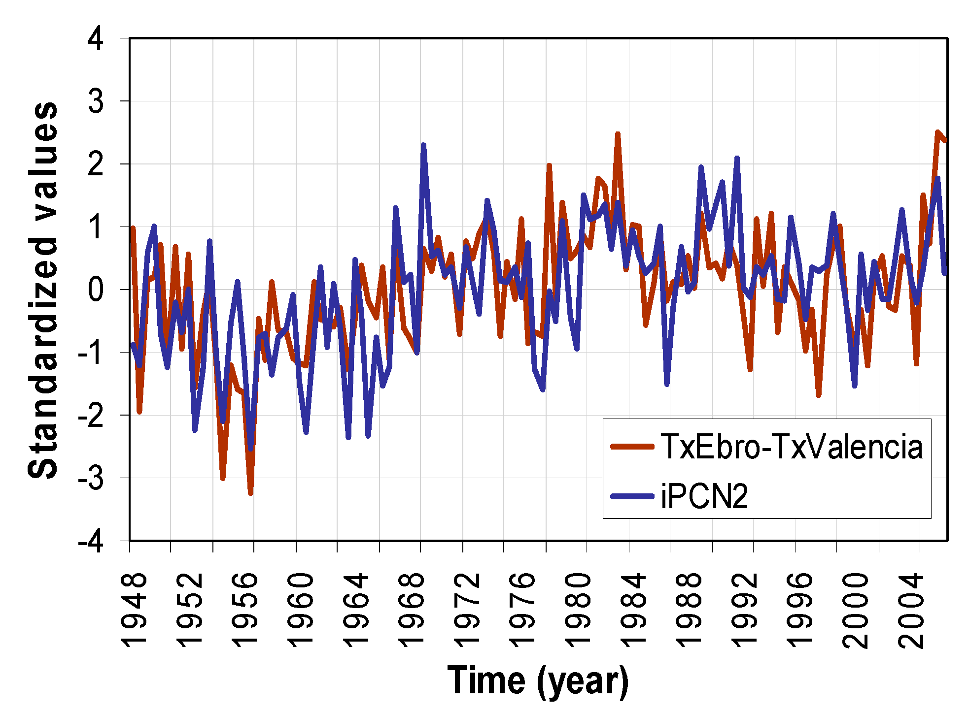
We also calculated the correlations between the indices iPCN1 and iPCN2 and the difference between the Tx and DTR at both observatories (TxEV, DTREV) (Table 2). As expected, the index iPCN2 correlates well with TXEV and DTREV (in contrast to iPCN1) and also with DTRE and DTRV. The time series of both iPCN2 and TXEV are close related (Figure 5).

5. Results

5.1. Synoptic Patterns Linked to iPCN2

The maps of Figure 6a,b show, for 10% of the Northern days with the lowest values of iPCN2 respectively, the spatial distribution of mean values for MSLP and Z500 anomalies and the Tx anomalies of the eastern IP. The negative SNAO signal becomes evident in the large area of low pressure in north Europe. From the strong westward pressure gradient over the IP we can expect a significant northerly wind (especially at the Ebro Observatory, thanks to its orographical conditions). The area of negative Z500 anomalies centred to the north of the Cantabrian Sea, which affects the northern part of the Iberian Peninsula, indicates the presence of cold air at high levels. Due to this, we can expect a reduction in the temperatures over the northern part of the IP.

On the contrary, the days with highest iPCN2 values (Figure 7) show how the Azores High expands over most of northern Europe—an indicator of a positive SNAO (the correlation between SNAO and iPCN2 is very significant (r = 0.52, >99%)). In this set of days, the positive Z500 anomalies over the IP are related to the presence of warm air at high levels. From these high Z500 values we can expect to see a rise in temperatures over the IP.

In the days with very negative values of iPCN2 (Figure 6a), the relative vorticity in the SW IP (VortSW) is slightly anticyclonic (slightly negative, with clockwise spin over the region around the grid point (7.5° W, 37.5° N)). Under these conditions, the flow in the Valencia area has western and north-western components and positive anomalies are recorded at Valencia and in the SE IP (Figure 6b), not just because of the summer sunlight but also due to the adiabatic compression the air is forced into as it descends from the high lands of inland IP. On the other hand, the area around the Ebro Observatory is more influenced by the negative anomalies of Z500 centred over the north of the Cantabrian Sea and the wind (relatively strong thanks to the steep westward pressure gradient) has a NW component and is linked to negative Tx anomalies (Figure 6b).

The opposite happens with high values of iPCN2 (Figure 7a). In this case, the relative vorticity (VortSW) is strongly positive and with counter-clockwise spin. The flow we expect to see in the SE IP is one from the second quadrant (Figure 7b), with a maritime route. This leads to a certain regulation of the maximum temperatures and also a slight increase in minimum temperatures, as seen in Table 2.

We calculated the average MSLP and Z500 anomalies (Figure 8) corresponding to the five months with the most negative values of iPCN2 for all the period 1948–2006 (August 1952, 1954, 1956, 1960 and 1963) and the five months with highest iPCN2 values (July 1969, 1989, 2006 and August 1991, 1998). We must pay attention to the sign of the average relative vorticity in the SW IP (VortSW). In the set of months with negative values of iPCN2 (all concentrated in the 1950s and 1960s), this relative vorticity was slightly anticyclonic; the opposite to what happened in the months with high values of iPCN2. As we can see, the influence of the iPCN2 index is sufficiently significant so as to leave a clearly-marked spatial ‘print’ on the average of several months. That is, it shows that the effects of iPCN2 are not only limited to specific days but that they are reflected in the average monthly values of several months.

5.2. Wind and Temperature at Ebro and Valencia Observatories with Respect to iPCN2 Index

So far, we have not used observational data relating to wind speed or direction. However, theoretical wind directions and speeds can be derived from the synoptic patterns we calculated corresponding to iPCN2 (Figure 6a and Figure 7a). Given the importance of the dominant wind direction on the Tx and DTR in our study area and since we also have observational meteorological data of wind direction and velocity at our two reference observatories (Ebro and Valencia), we shall now check, in an experimental way, the theoretical relationship we have calculated between the iPCN2 index and the wind velocity and direction in the areas around the two observatories.

At the Ebro Observatory, generally, the summer northerly wind is stronger at night and weaker around midday, contrary to the second quadrant wind. However, in the negative phase of iPCN2, the whole IP is under the influence of a strong westward pressure gradient (Figure 6a) and at the Ebro Observatory the northerly wind run (Figure 9a, blue line) is relatively strong during daytime hours (though less than at night), with similar values (on average) to the second quadrant wind (Figure 9a, blue dashed line). This also happens, though to a lesser degree, at Valencia (Figure 9b), which makes the daily wind run from the second quadrant decrease at both observatories (Figure 9b, blue dashed line).

Under these conditions, the maximum temperatures are low in the lower Ebro Valley (under the influence of negative Z500 anomalies centred over the north of the Cantabrian Sea) and therefore the cross-shore temperature gradient is very weak. As the cross-shore wind component towards the sea derived from the synoptic-scale conditions and enhanced by the orography of the lower Ebro Valley is very significant, the sea breeze will only reach the Ebro area on some days. On the other hand, in this case, the northerly wind is cool at the Ebro Observatory but warmer to the south of the coast, generating positive anomalies in maximum temperatures in the Tx along most of the coastline and pre-coastline of the SE IP (Figure 6b).

In the positive phase of iPCN2, the hourly wind run of the second quadrant at the Valencia Observatory is very close to its average value until midday. From then on, it is significantly higher than the average value (Figure 9b, black dotted line). This stronger evening breeze probably contributes to moderating the Tx. In this context, we found a good correlation between the Valencia Observatory DTR and the monthly frequency of sea breeze days (r = −0.27, >99%) (we considered breeze days to be only those in which a second quadrant wind was registered at midday but not in the early morning). The positive values of iPCN2 are linked to positive values of VortSW which is also linked to the frequency of sea breeze days (r = 0.31, >99%). Thus, when the iPCN2 index increases, so does the VortSW and with it the probability of the sea breeze reaching the Valencia Observatory, thus reducing the DTR.

However, at the Ebro Observatory, in the positive phase of iPCN2, the hourly wind run of the second quadrant (Figure 9a, black dashed line) is much weaker than the Southern days’ average, when the synoptic scale-pressure gradient enhances the sea breeze (Figure 9a, orange dashed line). This is so because in the early morning of the days with highly positive iPCN2 values, the wind from inland up the Ebro Valley, which blows in the night, is still active (Figure 9a, black line) owing to the favourable pressure gradient on a synoptic-scale and due to the channelling effect of the lower Ebro Valley’s orography. The synoptic pattern in this case, though, corresponds to a warm anticyclonic situation which will make daytime temperatures rise significantly. Only when these temperatures have reached relatively high values, will an increase in the wind from the second quadrant corresponding to the sea breeze be recorded. Only when there is a sufficiently strong cross-shore temperature gradient towards inland, will the resistance owing to the opposing synoptic-scale cross-shore wind component (towards the sea) be cancelled out [30] and will the Ebro Observatory be within the range of the sea breeze. In this case, the positive Tx anomalies spread throughout the northern part of the lower Ebro Valley and a little further northward of the Ebro Observatory, the temperature gradient almost disappears (Figure 4d), thus suggesting that, under these conditions, there is only a relatively weak penetration inland of the sea breeze (close to 25 km).

As it is in the pre-littoral area and in a valley whose orographical conditions strengthen both winds with northern components and those from the south, the relationship between wind and temperature at the Ebro Observatory is very complicated. One example of this is that, contrary to what we might expect, at the Ebro Observatory the Northern days are, on average, warmer than the Southern days. On the other hand, if we took into account only the cross-shore temperature gradient, we would expect on average, a stronger breeze on Northern days (at least on the warmest days) than on Southern days but in fact the opposite case occurs (Figure 9a: the run_2q is stronger on the Southern days than on the warmer days with iPCN2 values higher than 90th percentile). This is so, because during Southern days, the eastward pressure gradients, which are often related to the Iberian Peninsula thermal low, favour the influx of sea air and a fall in Tx and DTR. During Northern days, the opposite is true—large scale pressure gradients favour more the wind flow coming from inland, which can be very warmer (like in the positive phase of iPCN2) and makes the Tx and DTR increase significantly.

To sum up (

Table 3. Relation between iPCN2 and wind and Tx.

Index/Variable	Ebro Observatory			Valencia Observatory
	run_N	run_2q	TxE	run_N	run_2q	TxV
iPCN2PC10	$\uparrow \uparrow$	$\downarrow \downarrow$	$\downarrow \downarrow$	$\uparrow$	$\downarrow$	$\uparrow$
iPCN2PC90	$\uparrow$	$\downarrow$	$\uparrow \uparrow$	$\to$	$\uparrow$	$\downarrow$

): low iPCN2 values are related to a cold advection in the north IP which enhances the northerly wind in the lower Ebro Valley and makes the maximum temperatures fall, while positive anomalies are recorded at Valencia and in the SE IP. During the positive phase of iPCN2, the synoptic-scale conditions correspond to a warm anticyclone that favours the northerly flux in the Ebro Observatory, especially in the night and only when the cross-shore temperature gradient is high enough, will the sea breeze reach the Ebro Observatory (which means Tx and DTR increases); at the same time these conditions will favour a strengthened breeze at Valencia after midday which will stop the rise of Tx.

We focused on the wind run rather than on the average velocity because the wind run accounts not only for the strength with which the wind has been blowing from one specific direction but also for the duration of time the wind was blowing from that direction. The ‘average hourly wind run’ (Figure 9) refers to the average value obtained for each hour from the ‘wind run’ values corresponding to this hour for a specific set of days. For example, if on a specific day at a specific time, the wind does not blow with a positive northerly component, then the ‘run_N’ corresponding to this hour will be null, which would lower the average hourly ‘run_N’ for this hour.

5.3. Relationship between the Northerly Wind at Ebro Observatory and VortSW and the Tx in Valencia Region

The run_N measured at the Ebro Observatory has a very high sensitivity to large scale atmospheric conditions. One way to monitor some of the changes linked to the increase in the SNAO [21,29] and iPCN2 (Figure 5) and therefore, some of the effects of the progressive shift of the Azores High towards the north of Europe from the late 1960s onwards is by evaluating how the relationships between the northerly wind at the Ebro Observatory (run_N) and some significant variables such as the relative vorticity VortSW have changed with time. Studying how the relationship between the northerly wind and VortSW has changed over time can give us information on how the dominant direction of the northerly wind, which is related to the prevalence of certain synoptic patterns, has evolved over time in the SE of the IP and this is relevant given that, as we have seen, this direction influences decisively the Tx of this area.

On average, during the days with the most negative values of iPCN2 a cool northerly wind blows during the daytime at Ebro Observatory, while for very positive values of iPCN2, the wind only blows at night as it is substituted by a relatively weak and warm sea breeze in the daytime. Therefore, we should find negative correlations between iPCN2 and run_N on a daily level (r = −0.26, >99%). However, if we work with monthly values, we must bear in mind that there may be other kinds of synoptic patterns related to run_N which are different from those linked to iPCN2. In this case, the correlations obtained with monthly data will thus depend on the relative weight of iPCN2 within the total monthly run. In this sense, we must point out the good correlation between run_N and iPCN2 and SNAO (significative to 99%) in the period 1948–1967 (

Table 4. Linear correlations (monthly data).

Wind Run/Index	iPCN2	SNAO
run_N (1948–1967)	−0.59 **	−0.42 **
run_N (1968–2006)	−0.17	0

** (>99%)

), which indicates that in this period the episodes of northerly wind at the Ebro Observatory were linked more often to synoptic situations with very negative values of iPCN2 and SNAO. However, owing to the increase in the SNAO and iPCN2 indices, and to the dramatic drop in frequency of the situations with negative values of iPCN2 (and negative SNAO) from the end of the 1960s onward, the synoptic patterns related to cold advections and northerly winds were more and more often linked to positive values of the SNAO. For this reason, the correlation (using monthly data) between run_N and iPCN2 and between run_N and SNAO in the last decades of the 20th century became much weaker (Table 4).

The relation between run_N and VortSW on a monthly level is relevant as it gives us information regarding the kinds of synoptic patterns more often associated to the northerly wind at the Ebro Observatory, the possibility to see how these synoptic patterns have changed over time and the possibility to be able to contrast this changes in the context of the sharp rise of the index iPCN2 from the 1950s.

In the 1950s and 1960s, the northerly wind at the Ebro Observatory was linked to a decrease in VortSW (Figure 10), which is coherent with the strong negative correlation between iPCN2 and run_N in this period. From the end of the 1960s onward, the synoptic situations associated with the Ebro Observatory northerly wind were different as situations of negative iPCN2 and negative SNAO became less and less common. Owing to the strong increase in SNAO, the cold advections were more and more often linked to positive SNAO situations—characterized by having positive VortSW values in general [29]. This explains the positive correlation between VortSW and northerly wind in the last decades of the 20th century. Figure 10 shows how the correlation between run_N and VortSW changed throughout the second half of the 20th century from very significant values with a negative sign (r = −0.47, >99%) to positive values (r = 0.4, >95%). The change in sign of this correlation over time is a “footprint” of the changes which occurred during the second half of the 20th century. We can state that the correlation is significant, not just because of the wind itself but also due to the information it gives about the prevalence over time of certain atmospheric patterns.

In the 1950s and early 1960s, the run_N was linked to negative values of SNAO and iPCN2 and, therefore, to low values of the relative vorticity of the SW IP. This contributes to explain why, during this period, its relationship with the Tx at Valencia was weak (Figure 10). Although the northerly wind is cool, as it reaches the SE IP with a western component, the negative anomalies are weak, or even of positive sign. However, in the following decades, with the increase in SNAO and iPCN2, the atmospheric patterns linked to run_N became more and more associated to higher values of relative vorticity in the SW and, therefore, their capacity for making Tx fall in the SE was increased owing partly to the change in the wind route from a continental one to a marine route.

We must point out that the period during which the correlation between run_N and VortSW changed sign (from the 1950s to the beginning of the 1980s) (Figure 10) coincided with a change in the iPCN2 index (from negative to positive) (Figure 5), a change in the SNAO index (from negative to positive [21]), a large increase in the difference between the Ebro Observatory Tx with respect to those of the Valencia Observatory (Figure 5), a large increase in the Ebro Observatory DTR and a large fall in the Valencia Observatory DTR (Figure 11).

5.4. Estimation of DTR Trend (1954−1981) in the Ebro Region and the SE IP from the Indices iPCN1 and iPCN2

As the iPCN2 index experienced a strong increase between the mid 1950s and early 1980s (Figure 5), we should ask whether, from this increase, a statistically significant increase in the DTR of the Ebro Observatory region and a statistically significant decrease in the DTR of the SE IP can be inferred. Nevertheless, to explain these asymmetric trends from changes in atmospheric circulation, we cannot ignore the possible contribution of iPCN1, given its high statistical weight (it has been derived from the leading principal component PC1). With this aim, we calculated two linear regressions (with the 1948–2006 data) where the independent variables are iPCN1 and iPCN2 and the dependent variables are the average monthly values of the DTR of the Ebro Observatory region and the DTR of a region of the SE IP. We defined these two regions in such a way that the correlations obtained between the PC2 index and the DTR of each corresponding grid point of the Spain02 dataset (Figure 4b) are at maximum absolute values; this is a way to optimize the results as we have selected the areas where the relationship between DTR and PC2 is at its maximum. We use PC2 instead of iPCN2 because the spatial distribution of the correlations between DTR and PC2 has a better resolution than that corresponding to DTR and iPCN2. In this way, the Ebro Observatory region is defined as the set of grid points where the former correlation is over the +0.55 threshold (around the Ebro Observatory, Figure 4b). To select the SE IP and Valencia region close to the coast we chose the grid points with correlation values below the −0.1 threshold (the ones closest to the coast, Figure 4b).

We calculated the regressions after eliminating the trends in all the time series:

DTR(detrended) = a × iPCN1(detrended) + b × iPCN2(detrended) + c

(5)

Then, we calculated the ‘trended’ values of DTR with the previously calculated coefficients using the ‘trended’ indices:

DTR(trended) = a × iPCN1(trended) + b × iPCN2(trended) + c

(6)

We focused on the period 1954–1981 because from the early 1980s onward, both DTR trends were more synchronised and there was not such an important difference between them (Figure 11). From the calculation of both regressions, we found significant DTR trends (>95%) with reverted signs in both regions: positive in the Ebro region, which could account for 55% of the observed trend (0.8 °C/decade) and negative in the SE region closest to the coast which could account for 47% of the observed trend (−0.6 °C/decade). On the other hand, we saw that the contribution of iPCN1 to the DTR trend in the Ebro region is very small and in the SE region its effect is in the opposite direction in comparison with that of iPCN2, that is, it contributes to a positive DTR trend. If we only took into account the effects of iPCN2, then we could explain for 68% of the observed trend in the SE region close to the coast.

Hence, we conclude that the variations of the iPCN2 index during the second half of the 20th century (1954–1981) may contribute to explaining a significant part of the differential trend of the DTR in the Ebro Observatory region with respect to the SE IP region closest to the coast.

On the other hand, there could be other processes responsible for explaining the remaining percentages of the observed trends, apart from those derived from the possible influence of the heat island effect on temperatures on the littoral areas of SE IP [20]. However, it is also possible that the changes in atmospheric circulation described by these indices are more significant than the trends that we have calculated. Our calculations are only based on four sets of large-scale variables (Z500, Z500–Z100, MSLP and sea level relative vorticity) and their capacity to describe processes on a mesoscale level is limited.

6. Discussion and Conclusions

We carried out an initial classification between ‘Northern days’ and ‘Southern days’ setting out from regional aspects regarding the kind of wind to be expected in the region around the Ebro Observatory. This classification is also applicable on a larger scale—particularly over the Iberian Peninsula [21,29].

We calculated a PCA from a set of variables which come from the NCEP reanalysis (T850, VortSW, VortNW) and from observation data (Tx and DTR of Ebro and Valencia Observatories) and then we obtained the indices iPCN1 and iPCN2 from reanalysis data (MSLP, Z500, Z500–Z1000 and sea level relative vorticity).

In the positive phase of iPCN2, the north-westerly flow makes the Tx and DTR increase in the lower Ebro valley as it corresponds to a warm anticyclonic situation with clear skies and warm air at high levels. Under these conditions, the Tx in the inland IP increase significantly which make the Ebro Observatory Tx increase as the flow displaces the continental air mass near the coast. But these conditions are, in turn, responsible for a slight fall in the same variables on the SE coast of the IP due to a greater exposure there to northerly air with a maritime route.

The opposite case happens in the negative phase of iPCN2. Here, the temperatures tend to fall inland as these conditions are not anticyclonic ones but correspond to an influx of air from higher latitudes at high levels in combination with northerly wind at low levels due to the presence of a strong westward pressure gradient. This air is much colder than on average at high levels and prevents the maximum temperatures from increasing—especially in the northern part of the IP but not on the SE and Valencia coast where this wind comes from inland (‘ponent’) and is therefore warmer, due to its crossing of the IP under high insolation conditions and to the adiabatic compression due to the loss of altitude. Accordingly, we found at the Valencia Observatory, very significant correlations between the daily westerly wind run (direction from the third and fourth quadrant) and the iPCN2 index and VortSW (r = −0.41, >99% and r = −0.42, >99%, respectively) in the period (1997–2006). The days with westerly wind can register very high temperature levels in the SE IP and Valencia region coast. This explains why we also found a significant correlation (r = −0.21, >99%) between the iPCN2 index and the frequency of days with Tx > Tx90 (90th percentile of the Tx of each station) in the stations of this area.

In the 1950s and early 1960s, during the Northern days (the frequency of which was significantly higher than usual [29]), the iPCN2 and the SNAO values were frequently negative, restraining maximum temperatures in northern IP due to the northerly flow linked to a marked westward pressure gradient and maintaining a reduced DTR in the area around the Ebro Observatory. However, in the same period, these negative values of iPCN2 and the consequent negative values of the relative vorticity in the SW IP contributed to increasing the Tx and DTR in the area around the SE IP and Valencia region close to the coast and also increased the frequency of days with westerly winds (‘ponentades’). So, we can conclude that in the 1950s and early 1960s, the atmospheric circulation enhanced the frequency of westerly flow and the probability of extreme temperatures in that region. In the 1950s and early 1960s, therefore, the maximum temperatures and DTR at the Ebro and Valencia Observatories showed a certain convergence.

The increase detected in the iPCN2 index from the late-1960s onward contributes to explaining why, from the late 1960s to about 1980, the Tx and the DTR in both regions (Ebro Observatory and Valencia and the SE area close to the coast) showed a greater and greater divergence. The subsequent increase in the relative vorticity in the SW IP decreased the influence of inland winds at the Valencia Observatory and in the SE IP closest to the coast and enhanced the frequency of sea breezes but at the same time the enhanced anticyclonic conditions contributed to increasing the Tx and DTR in the area around the Ebro Observatory. Thus, the general increase in Tx seen at the end of the 20th century related to the current climate change was strengthened in the lower Ebro Valley owing to the shift of the Azores High towards the NE and, at the same time, it was weakened in the littoral and pre-littoral areas of the SE IP.

There are several studies [17,18] that show a decrease of the DTR in the SE of the IP in the second part of the 20th century but we disagree with their proposed explanation—in particular due to the fact that the decrease occurs mainly between the 1950s and early 1980s, before the current climate change. These studies assume that the DTR drop could be explained from a rise in the minimum temperatures but we checked that the DTR drop from the late-1960s to around 1980 in the SE IP closest to the coast in summer, is mainly due to a steeper drop in the maximum temperatures than in the minimum ones. Thus, from the 1980s to the beginning of the 21st century, the DTR does not show a significant trend, which is in line with what happens globally [6].

The steep rise of the iPCN2 and SNAO indices (highly correlated during the period 1948–2006, r = 0.52, >99%) of the late 1960s had two important cumulative effects on the maximum temperatures of the Valencia region and the SE IP: on the one hand, there was a drop in the frequency of days with westerly wind and, on the other, the northern cold advections in summer tended to be more centred on the eastern IP [29]. The cold advections in the eastern IP are related to blocking situations in northern Europe, which force air at higher latitudes to move to lower latitudes. These blockings are usually related to strongly positive values of the SNAO index. One specific case is that of the cold advections over the Gulf of Lion [29]. Furthermore, these cold advections were frequently related to an increase in the total cloud cover in the SE of the Iberian Peninsula [29] which probably also contributed to lowering the Tx in the SE IP and Valencia region. All this contributes to explaining why some studies have emphasised the relatively low rise of maximum temperature seen in the eastern and SE Mediterranean area of the IP in the second half of the 20th century after removing urbanization effects [20,34].

References

1. Intergovernmental Panel on Climate Change (IPCC). Climate Change 2013: The Physical Science Basis. Contribution of Working Group I to the Fifth Assessment Report of the Intergovernmental Panel on Climate Change; Stocker, T.F., Qin, D., Plattner, G.-K., Tignor, M., Allen, S.K., Boschung, J., Nauels, A., Xia, Y., Bex, V., Midgley, P.M., Eds.; Cambridge University Press: Cambridge, UK; New York, NY, USA, 2013. [Google Scholar]
2. Brunet, M.; Jones, P.D.; Sigró, J.; Saladié, O.; Aguilar, E.; Moberg, A.; Della-Marta, P.M.; Lister, D.; Walther, A.; López, D. Temporal and spatial temperature variability and change over Spain during 1850–2005. J. Geophys. Res. 2007, 112, D12117. [Google Scholar] [CrossRef]
3. Jones, P.D.; New, M.; Parker, D.E.; Martin, S.; Rigor, I.G. Surface air temperature and its changes over the past 150 years. Rev. Geophys. 1999, 37, 173–199. [Google Scholar] [CrossRef]
4. Zwiers, F.W.; Weaver, A.J. The Causes of 20th Century Warming. Science 2000, 290, 2081–2083. [Google Scholar] [CrossRef] [PubMed]
5. Easterling, D.R.; Horton, B.; Jones, P.D.; Peterson, T.C.; Karl, R.R.; Parker, D.E.; Salinger, M.J.; Razuvayev, V.; Plummer, N.; Jamason, P.; et al. Maximum and minimum temperature trends for the globe. Science 1997, 277, 364–367. [Google Scholar] [CrossRef]
6. Vose, R.S.; Easterling, D.R.; Gleason, B. Maximum and minimum temperature trends for the globe: An update through 2004. Geophys. Res. Lett. 2005, 32, L23822. [Google Scholar] [CrossRef]
7. Brunet, M.; Aguilar, E.; Saladié, O.; Sigró, J.; López, D. Warming phases in long term Spanish temperature change. In Proceedings of the American Meteorological Society 13th Symposium on Global Change and Climate Variations, Orlando, FL, USA, 13–17 January 2002. [Google Scholar]
8. Esteban-Parra, M.J.; Pozo-Vazquez, D.; Rodrigo, F.S.; Castro-Diez, Y. Temperature and precipitation variability and trends in Northern Spain in the context of the Iberian Peninsula climate. In Mediterranean Climate: Variability and Trends; Bolle, H.J., Ed.; Springer: New York, NY, USA, 2003; pp. 259–276. [Google Scholar]
9. Oñate, J.J.; Pou, A. Temperature variations in Spain since 1901: A preliminary analysis. Int. J. Climatol. 1996, 16, 805–816. [Google Scholar] [CrossRef]
10. Rodríguez-Puebla, C.; García-Casado, L.A.; Frías, M.D. Trend and interannual variations in air temperature over Iberian Peninsula. In Proceedings of the American Meteorological Society 13th Symposium on Global Change and Climate Variations, Orlando, FL, USA, 13–17 January 2002. [Google Scholar]
11. Brunet, M.; Sigró, J.; Saladié, O.; Aguilar, E.; Jones, P.D.; Moberg, A.; Walther, A.; López, D. Spatial patterns of long-term Spanish temperature change. Geophys. Res. Abstr. 2005, 7, 04007. [Google Scholar]
12. Brunet, M.; Saladié, O.; Jones, P.D.; Sigró, J.; Aguilar, E.; Moberg, A.; Walther, A.; Lister, D.; López, D.; Almarza, C. The development of a new daily adjusted temperature dataset for Spain (1850–2003). Int. J. Climatol. 2006, 26, 1777–1802. [Google Scholar] [CrossRef]
13. Abaurrea, J.; Asín, J.; Erdozain, O.; Fernández, E. Climate variability analysis of temperature series in the Medium Ebro River Basin. In Detecting and Modelling Regional Climate Change; Brunet, M., López, D., Eds.; Springer: New York, NY, USA, 2001; pp. 109–118. [Google Scholar]
14. Galan, E.; Cañada, R.; Fernández, F.; Cervera, B. Annual temperature evolution in the southern plateau of Spain from the construction of regional climatic time series. In Detecting and Modelling Regional Climate Change; Brunet, M., López, D., Eds.; Springer: New York, NY, USA, 2001; pp. 119–131. [Google Scholar]
15. Horcas, R.; Rasilla, D.; Fernández, F. Temperature variations and trends in the Segura River Basin. An exploratory analysis. In Detecting and Modelling Regional Climate Change; Brunet, M., López, D., Eds.; Springer: New York, NY, USA, 2001; pp. 133–142. [Google Scholar]
16. Morales, C.G.; Ortega, M.T.; Labajo, J.L.; Piorno, A. Recent trends and temporal behavior of thermal variables in the region of Castilla-Leon (Spain). Atmósfera 2005, 18, 71–90. [Google Scholar]
17. Miró, J.; Estrela, M.J. Tendencia de la temperatura en los meses de julio y agosto en la comunidad Valenciana en las últimas décadas: Cambios en la frecuencia de días calurosos. In El Clima Entre el Mar y la Montaña; García, J.C., Liaño, C., de Arróyabe, P.F., Garmendia, C., Rasilla, D., Eds.; Serie A, No. 4; Publicaciones de la Asociación Española de Climatología (AEC); Universidad de Cantabria: Santander, Spain, 2004. [Google Scholar]
18. Miró, J.; Estrela, M.J.; Millan, M. Summer temperature trends in a Mediterranean area (Valencia region). Int. J. Climatol. 2006, 26, 1051–1073. [Google Scholar] [CrossRef]
19. Quereda, J.; Montón, E.; Escrig, J. Las tendencias climáticas de la región mediterránea ¿cambio o estabilidad? Revista Valenciana d’Estudis Autonòmics 1999, 27, 117–152. [Google Scholar]
20. Quereda, J.; Montón, E.; Quereda, V.; Mollá, B. Significant Climate Warming (1950–2013) in the Spanish Mediterranean: Natural Trend or Urban Heat Island (UHI). Tethys 2016, 13, 11–20. [Google Scholar]
21. Favà, V.; Curto, J.J.; Llasat, M.C. Relationship between the summer NAO and maximum temperatures for the Iberian Peninsula. Theor. Appl. Climatol. 2015, 126, 77–91. [Google Scholar] [CrossRef]
22. Hurrell, J.W.; Folland, C.K. A Change in the Summer Circulation over the North Atlantic; CLIVAR Exchanges No. 25; International CLIVAR Project Office: Southampton, UK, 2002; pp. 52–54. [Google Scholar]
23. Folland, C.K.; Knight, J.; Linderholm, H.W.; Fereday, D.; Ineson, S.; Hurrell, J.W. The Summer North Atlantic Oscillation: Past, present and future. J. Clim. 2009, 22, 1082–1103. [Google Scholar] [CrossRef]
24. Bladé, I.; Liebmann, B.; Fortuny, D.; van Oldenborgh, G.J. Observed and simulated impacts of the summer NAO in Europe: Implications for projected drying in the Mediterranean region. Clim. Dyn. 2011, 39, 709–727. [Google Scholar] [CrossRef]
25. National Centers for Environmental Prediction/National Weather Service/NOAA/U.S. Department of Commerce; Research Data Archive at the National Center for Atmospheric Research, Computational and Information Systems Laboratory. NCEP/NCAR Global Reanalysis Products, 1948-Continuing. Updated Monthly; 1994. Available online: http://rda.ucar.edu/datasets/ds090.0/ (accessed on 6 September 2013).
26. Herrera, S.; Gutiérrez, J.M.; Ancell, R.; Pons, M.R.; Frías, M.D.; Fernández, J. Development and analysis of a 50-year high-resolution daily gridded precipitation dataset over Spain (Spain02). Int. J. Climatol. 2012, 32, 74–85. [Google Scholar] [CrossRef] [Green Version]
27. Curto, J.J.; Also, E.; Pallé, E.; Solé, J.G. Sunshine and synoptic cloud observations at Ebro Observatory, 1910–2006. Int. J. Climatol. 2009, 29, 2183–2190. [Google Scholar] [CrossRef]
28. Turco, M.; Llasat, M.C. Trends in indices of daily precipitation extremes in Catalonia (NE Spain), 1951–2003. Nat. Hazards Earth Syst. Sci. 2011, 11, 3213–3226. [Google Scholar] [CrossRef] [Green Version]
29. Favà, V.; Curto, J.J.; Llasat, M.C. Regional differential behaviour of maximum temperatures in the Iberian Peninsula regarding the Summer NAO in the second half of the twentieth century. Atmos. Res. 2016, 182, 319–334. [Google Scholar] [CrossRef]
30. Miller, S.; Keim, B. Synoptic-scale controls on the sea breeze of the Central New England Coast. Weather Forecast. 2002, 18, 236–248. [Google Scholar] [CrossRef]
31. Holton, J.R. An Introduction to Dynamic Meteorology, 3rd ed.; International Geophysics Series; Academic Press: Cambridge, MA, USA; Elsevier Science: New York, NY, USA, 1992; Volume 48. [Google Scholar]
32. The NCAR Command Language (Version 6.1.1) [Software]. UCAR/NCAR/CISL/VETS: Boulder, Colorado. Available online: http://dx.doi.org/10.5065/D6WD3XH5 (accessed on 29 January 2012).
33. Sánchez-Lorenzo, A.; Sigró, A.; Calbo, J.; Martin-Vide, J.; Brunet, M.; Aguilar, E.; Brunetti, M. Efectos de la nubosidad e insolación en las temperaturas recientes de España. In Cambio Climático Regional y Sus Impactos; Sigró, J., Brunet, M., Aguilar, E., Eds.; Serie A, No. 6; Publicaciones de la Asociación Española de Climatología (AEC); Universitat Rovira i Virgili: Tarragona, Spain, 2008; pp. 273–284. ISBN 978-84-612-6051-5. [Google Scholar]
34. Quereda, J.; Montón, E.; Escrig, J. El Cambio Climático en las Regiones de Valencia y Murcia: La Sombra Analítica de un Auténtico Troyano; Investigaciones Geográficas; Instituto Universitario de Geografía, Universidad de Alicante: Alicante, Spain, 2009; Volume 49, pp. 109–127. ISSN 0213-4691. [Google Scholar]
Figure 1. (a) Position of the two observatories. Ebro (40.82° N, 0.49° E) and Valencia (39.49° N, 0.47° W); (b) Relief map of the lower Ebro Valley.
Atmosphere 09 00042 g001
Figure 2. Maximum absolute values of the correlations between TxValencia and the relative vorticity difference between two points (daily data).
Atmosphere 09 00042 g002
Figure 3. Correlations of the variables with PC1 and PC2 (daily data 1948–2006).
Atmosphere 09 00042 g003
Figure 4. (a) Daily correlations between Tx and PC2 (top blue cross—Ebro Observatory, bottom blue cross—Valencia Observatory); (b) Daily correlations between DTR and PC2; (c) Average value of maximum temperatures in lower Ebro Valley (PC2 < 10th percentile) (1996–2006); (d) Average value of maximum temperatures in lower Ebro Valley (PC2 > 90th percentile) (1996–2006). White point indicates the location of the Ebro Observatory, to the NW of the Ebro delta.
Atmosphere 09 00042 g004
Figure 5. Time series of TxEbro-TxValencia (brown) and iPCN2 (blue).
Atmosphere 09 00042 g005
Figure 6. (a) MSLP (hPa) and Z500 (gpm) anomalies (iPCN2 < 10th percentile); (b) Average value of the Tx anomalies in the east IP (iPCN2 < 10th percentile). The positive Tx anomalies of the SE IP are to the right of the thick line. Black arrows represent the direction of the air flux.
Atmosphere 09 00042 g006
Figure 7. (a) MSLP (hPa) and Z500 (gpm) anomalies (iPCN2 > 90th percentile); (b) Average value of the Tx anomalies in the east IP (iPCN2 > 90th percentile). The negative Tx anomalies of the SE IP are to the right of the thick line. Black arrows represent the direction of the air flux; in the Ebro region, it depends a lot on the distance from the coast since the sea breeze arrives to sites near the coast but inland up the Ebro valley we can find wind blowing from the northwest.
Atmosphere 09 00042 g007
Figure 8. (a) MSLP (hPa) and Z500 (gpm) anomalies for the 5 months with the most negative values of iPCN2; (b) MSLP (hPa) and Z500 (gpm) anomalies for the 5 months with the most positive values of iPCN2.
Atmosphere 09 00042 g008
Figure 9. (a) For Ebro Observatory, average hourly wind run for iPCN2 < 10th percentile (run_N in blue line and run_2q in blue dashed line) and for iPCN2 > 90th percentile (run_N in black line and run_2q in black dashed line. Run_N corresponds to the wind run of the wind with positive northerly component and run_2q to the wind run of the second quadrant wind), average run_2q in Southern days (orange dashed line) and average run_2q in Northern days (orange line). The average hourly wind run was computed by dividing for each hour, the integration of the wind run from one specific direction throughout the days of each sample and the number of days of that sample. (b) The same for Valencia but here it is shown the average run_2q (orange dashed line) of the whole set of days.
Atmosphere 09 00042 g009
Figure 10. Correlation between run_N and TxValencia and VortSW (28-month window).
Atmosphere 09 00042 g010
Figure 11. Time series of DTR at Ebro (blue) and SE close to the coast (brown).
Atmosphere 09 00042 g011