Assessing the Skill of Convection-Allowing Ensemble Forecasts of Precipitation by Optimization of Spatial-Temporal Neighborhoods

1
College of Meteorology and Oceanography, National University of Defense Technology, Nanjing 211101, China
2
The office of Nanjing Joint Center of Atmospheric Research (NJCAR), Nanjing 210009, China
3
PLA Troop 92664, Haiyang 265100, China
*
Author to whom correspondence should be addressed.
Atmosphere 2018, 9(2), 43; https://doi.org/10.3390/atmos9020043
Submission received: 18 December 2017
/
Revised: 17 January 2018
/
Accepted: 25 January 2018
/
Published: 27 January 2018
(This article belongs to the Section Meteorology)
Abstract
:The current neighborhood probability (NP) method mainly considers the spatial displacement error in high-resolution precipitation forecasts, but the problem of the forecast time exceeding or lagging behind the observed field has not been properly solved. Therefore, a temporal factor was introduced into the NP method in this paper, and precipitation forecasts were evaluated in different spatial-temporal neighborhoods based on the improved NP method and fractions skill score (FSS), combined with the relative operating characteristic (ROC) curve. The results indicated that the forecasting accuracy of the ensemble forecast was higher than the control forecast. The neighborhood ensemble probability (NEP) and probability matched mean (PMM) methods were superior to the traditional ensemble mean (EM) method in forecasting heavy rainfall, which compensated for the limitations of the heavy rainfall forecasting ability of EM. For such squall line processes, a spatial scale of 15–45 km neighborhood radius could effectively rectify the displacement error of precipitation. There was a corresponding relationship between temporal scale and rainfall intensity in convective-scale precipitation forecast, so the temporal uncertainty of different levels of precipitation could be captured by different temporal scales. The spatial and temporal scales had interdependent influences on precipitation forecast effects, which could be affected by the intrinsic spatial-temporal scale of convective-scale weather systems. The improved NP method could simultaneously reflect the spatial and temporal uncertainties of convective-scale precipitation forecasts in high-resolution models, achieving a comprehensive assessment of spatial-temporal scale and providing probabilistic forecast results that match different levels of precipitation.
1. Introduction
As the demand for accurate forecasting of extreme weather is constantly increasing, convective-scale weather forecasting is becoming increasingly important. The refined convective-scale weather forecast is facing notable challenges due to its small spatial-temporal scale and the high non-linearity of the dynamic and physical processes. Therefore, it is of vital importance to develop high-resolution convection-allowing ensemble forecasts. In recent years, the UK Met Office [1] has conducted convection-allowing ensemble forecast experiments using downscaling and short perturbation rapid cycling methods. In Germany, scholars used the Consortium for Small Scale Modeling (COSMO) model to conduct some convection-allowing ensemble forecast experiments [2,3]. In America, the National Center for Atmospheric Research (NCAR) and the Center for Analysis and Prediction of Storms (CAPS) conducted a series of convection-allowing ensemble forecast experiments [4,5,6,7,8,9,10] focusing on the evaluation of precipitation and extreme weather indications, which aroused interest in the study of convection-allowing ensemble forecasts. NCAR carried out continuous convection-allowing ensemble forecast experiments and case studies over the Conterminous United States (CONUS) with an inner 3-km resolution, and had a preliminary analysis on the forecast results [4,5]. CAPS constructed the ensemble forecast system with 4 km-resolution ensemble members produced by initial conditions (IC), physical process and model perturbations, and carried out sensitivity tests and verifications related to the physical process and post-processing methods [6,7,8,9,10]. These studies indicated that convection-allowing ensemble forecasts could improve forecasting accuracy to a certain extent, and provide useful guidance for high-impact convective weather events. In China, Li et al. [11], Zhuang et al. [12], and Cai et al. [13] also conducted convection-allowing ensemble forecasts using different methods of IC perturbations and physical process perturbations, which provided theoretical evidence for the further development of perturbation techniques applicable to convection-allowing ensemble forecasts.
Further, the evaluation of high-resolution model forecasts is of great significance. As resolution is continuously increasing, the traditional skill scores used to test the performance of coarse-resolution models face problems in the evaluation of high-resolution models. Firstly, the traditional skill scores usually require correspondence between forecasted and observed events on a grid scale. However, the lack of dense spatial observations results in the subjectivity of the high-resolution model assessments produced by the traditional skill scores [14]. Secondly, high-resolution convection-allowing forecast models usually produce small displacement errors in precipitation for physical processes, and the parametric schemes in convective-scale weather are not entirely clear. When the traditional point-to-point verification methods are applied to high-resolution forecast result assessments, ignoring the displacement errors will result in poor objectiveness scores [15]. Therefore, traditional skill scores are defective when evaluating the forecasting capability for precipitation in high-resolution models. There is a dilemma in that, although it reveals the spatial-temporal structure information of convective weather systems, the scoring of high-resolution models is even poorer than that of coarse-resolution ones [16].
For the above problems, Ebert [17] proposed a neighborhood post-processing approach, and elaborated the basic framework for high-resolution precipitation verification. With respect to post-processing, to improve the forecasting accuracy of convective precipitation events with high-resolution models, Roberts and Lean [18] proved that more skillful precipitation forecasts could be produced by selecting an appropriate spatial scale based on the neighborhood method. Weusthoff et al. [19] used the neighborhood method to assess the performance of the high-resolution model and its corresponding low-resolution model at different spatial scales, showing that the high-resolution model had a better forecasting capability. On the topic of verification, Schwartz et al. [15] applied the neighborhood method to generate the results of probabilistic quantitative precipitation forecasts (QPFs) using the CAPS high-resolution ensemble forecast dataset, and verified its effect on probabilistic forecasts at different spatial scales. Clack et al. [20] used the area under the relative operating characteristic (ROC) curves at different spatial scales to measure the probabilistic QPFs. Pan et al. [21] evaluated the forecasting capability of three models at different spatial scales with the neighborhood method, and found that it was not reasonable to use a large neighborhood range to assess local precipitation. The forecast time ahead or lag of the convective-scale weather is as important as the spatial displacement error, however, there has been little previous work focusing on the temporal-scale effect of precipitation forecasts in high-resolution models.
Therefore, this study introduced the temporal factor into the neighborhood probability (NP) method, and conducted a convection-allowing ensemble forecast for a strong squall line. To optimize precipitation forecasts and improve forecasting accuracy of convective precipitation events, the precipitation forecasts were evaluated in different spatial-temporal neighborhoods based on the improved NP method and fractions skill score (FSS), combined with the ROC curves. Section 2 describes the convective-scale weather case and the design of the experiment. Section 3 introduces the experimental methods, especially the improved NP method and FSS. Section 4 briefly analyzes the results of the deterministic precipitation forecast. Section 5 presents the analysis of the probabilistic forecast results of different spatial-temporal neighborhoods. The summary and discussion are given in Section 6.
2. Case and Experimental Design
A wide-range severe convective weather process occurred over the Jianghuai region of China from 30 July to 31 July 2014. Affected by the weather process, Henan, Anhui, and Jiangsu provinces suffered thunderstorms, gales, and other short (but strong) convective weather conditions. The gales led to numerous houses being damaged or collapsed, and caused deaths in Henan Province. Some areas of Jiangsu Province suffered severe and local waterlogging due to the rainstorm. A strong east–westward squall line swept from north to south over the north-central part of Jiangsu and Anhui provinces, from 0600 UTC to 1100 UTC, 30 July 2014, which caused gusts of more than 14 m/s in Mingguang City and heavy rain in Changfeng Town (with hourly precipitation reaching 75 mm).
The experiment was conducted with the mesoscale nonhydrostatic model WRFV3.6 (developed by National Center for Environmental Prediction, NCEP, College Park, MD, USA), adopting a bidirectional dual nesting scheme. The domain setting is shown in Figure 1, encompassing approximately two-thirds of China. The nesting grid resolutions were 9 km and 3 km, respectively, and the internal domain met the high-resolution requirements of the convection-allowing forecast model. The center was located at 35° N, 115° E, and the horizontal grid points were 367 × 268 in the outer domain (d01) and 292 × 256 in the nest (d02). The vertical direction was non-equidistantly divided into 42 levels at both domains. Table 1 lists the Weather Research Forecasting (WRF) model’s basic physical parameterizations that were shared by all ensemble members. The outer and inner domains used the same physical schemes, except that cumulus parameterization was turned off in the inner domain.
The experiment included the breeding and forecasting phase. In the breeding phase, the model was operated from 1800 UTC, 28 July 2014 to 1800 UTC, 29 July 2014, only in the outer domain (d01) with 35 IC perturbation members generated by the breeding growth modes (BGM) method with a 6-h breeding cycle. To obtain the IC perturbation, the root-mean-square error (RMSE) between the forecast and analysis was calculated. Random numbers, which were distributed uniformly between 0 and 1, were added to this RMSE to obtain the initial perturbations. After one breeding cycle finished, a Global Forecast System (GFS) analysis in the current moment was introduced as the background field to rescale the perturbations by dynamic adjustments [11]. After the breeding finished, the ensemble forecast with the IC perturbation members applied the bidirectional dual nesting scheme over the whole domain (Figure 1). The forecast was initialized at 1800 UTC, 29 July 2014, and valid at 0000 UTC, 31 July 2014. The control forecast was initialized without perturbations.
The model was driven with the NCEP GFS 0.5° × 0.5° grid analysis data. They were used for both the initial conditions at 1800 UTC, 28 July 2014, and the boundary conditions throughout. Notably, the use of analyses for boundary conditions was to enable a more accurate forecast, and then for a more thorough discussion of the improvements provided by the methods (Section 3) for precipitation forecasts, especially for heavy rainfall. The China Hourly Merged Precipitation Analysis 0.1° × 0.1° grid data from the National Meteorological Information Center (NMIC) was used as the observed field for comparison.
3. Methods
3.1. Probability Matched Mean (PMM) Method
As a traditional post-processing method for the results of ensemble forecasts, the ensemble mean (EM) method can integrate the information of all the ensemble members. However, previous studies [21,22] have shown that after simple averaging, the forecast values at heavy rainfall thresholds are smoothed out. As a result, the EM method tends to eliminate heavy precipitation and indicates relatively light rainfall. Therefore, the probability matched mean (PMM) method [23] was used to synthesize the results of the ensemble forecast in this study. As an improved EM method, the PMM takes into account the characteristics of rapid spatial-temporal changes in the convective-scale weather system, synthesizes the grid-point forecast values of all the ensemble members, emphasizes the forecast information at heavy rainfall thresholds, and also ensures the basic structure of the traditional EM field [7,23,24,25,26]. The PMM precipitation forecasting field was generated as follows:
- (1)
- The grid-point precipitation values of all the ensemble members (Nm) are sorted into a monotonically decreasing order, named sequence 1.
- (2)
- The forecast values are selected at every Nm interval from sequence 1 to obtain sequence 2, of which the grid-point number is the same as the total number of grid points in the study area. There are altogether Nm kinds of equal probability cases in sequence 2. The authors chose the ith case randomly, where i = 1, 2, 3, ···, Nm.
- (3)
- The forecast values in the EM field are ranked from highest to lowest to obtain sequence 3, with the location of each value stored along with its rank.
- (4)
- The largest precipitation value from sequence 2 is reassigned to the grid-point location of the corresponding largest EM value from sequence 3, and so on, until the lowest value from sequence 2 is reassigned to the last location of the minimum EM value from sequence 3. Finally, the PMM precipitation forecasting field is obtained. Here, sequence 3 plays a bridge role in providing the location of each value for the PMM sequence.
3.2. NP Method with Temporal Factors
In general, ensemble forecasts provide probabilistic QPFs based on the precipitation information for each grid point of all the ensemble members. In this original method, each grid-point value is considered as independent, regardless of the continuity of the precipitation’s spatial-temporal distribution. Considering the high non-linearity of convective-scale weather systems and small-scale spatial-temporal uncertainties produced by high-resolution forecast models, the interaction between grid points cannot be neglected. Therefore, the NP method [15,27,28] is introduced to post-process the ensemble forecast results, integrating all the precipitation values in the neighborhood range, and producing a more reasonable distribution of the precipitation probability. Figure 2 shows the schematic diagram used to obtain the precipitation probability produced by the NP method.
First, let denote an event threshold (e.g., q = 1.0 mm/h) and the deterministic forecast at each grid point (, where represents the grid point of longitude and represents the grid point of latitude) for each ensemble member. Then, the binary probability (BP) of event occurrence at the () grid point is simply:
The observed field is similar to Equation (1), which is true for all the deterministic forecast.
After creating binary fields (Figure 2), the BP values in the neighborhood range (e.g., r = 15 or 30 km) are averaged to obtain the NP field, as shown in Equation (2).
represents the number of grid points contained in the radius of neighborhood (r). Figure 2 shows that the neighborhood range consists of 21 boxes and has 9 shaded boxes that exceed the specified threshold, so = 42.86%, at the central grid box in this example. Therefore, the NP method can be applied to produce the probability fields of every ensemble member, control forecast, and observed precipitation, and to compare their results directly.
The current research studies on the neighborhood method mainly focus on the spatial neighborhood, and less on the temporal neighborhood. However, it is equally crucial to predict the time of heavy precipitation for catastrophic convective precipitation events. Therefore, the phenomenon of forecast time ahead or lag should be taken into consideration. The study introduced the temporal factor into the NP method, considered the temporal difference of precipitation, and produced more reasonable probability forecast results. The proposed temporal neighborhoods were 3 h and 5 h (taking the occurrence moment as an example, considering the moment and ), because a longer temporal neighborhood would obscure the research significance of short and heavy precipitation in convective-scale weather systems. Then, the neighborhood probability of the grid point should be rewritten. Equation (2) becomes
Here, represents the number of considered times, and selects 1, 3, and 5 in Equation (3). The remaining symbols are the same as Equation (2).
At the same time, the neighborhood ensemble probability (NEP), generated by averaging the neighborhood probabilities of all the ensemble members, is one of the important indexes for comprehensively examining the performance of the ensemble forecast system and NP method.
3.3. FSS with Temporal Factors
Roberts et al. [18] defined the FSS for the NP method. The forecast assessment of this score included spatial-scale information, but not temporal-scale information. This paper introduced the temporal-scale information into the formula for the score to produce an improved FSS, which can simultaneously consider the spatial and temporal scales information.
Firstly, the neighborhood probabilities of each grid point in the forecast field and observed field are calculated by the NP method at the radius of neighborhood () and the time (), and then the mean square error (MSE) of forecast and observed fields is defined as the fractions Brier score (FBS) in Equation (5).
when the temporal neighborhoods are 1 h, 3 h, and 5 h, the corresponding forecast times are , , and , respectively. However, the observed time remains for the verification of the forecast performance considering temporal uncertainties.
Next, because FBS is a negative score index, the smaller the FBS value, the better the probabilistic forecast technique. If the neighborhood probabilities of forecasted and observed fields do not overlap spatially at any time, the MSE is maximized. Therefore, the effect of the probabilistic forecast is the worst in Equation (6).
Lastly, the FBS is converted to the FSS to eliminate the effect of no precipitation grid points in Equation (7). The FSS ranges continuously between 0 and 1, and the probabilistic forecast technique is optimal when the FSS = 1.
4. The Deterministic Forecast Results
4.1. Domain Total Precipitation
Figure 3 shows the evolution of total hourly precipitation in the internal domain (d02) over the forecast time. The first three hours represented the spin-up time of the model, therefore the precipitation was less than observed. In terms of precipitation tendency, the ensemble forecast was in fairly good agreement with the observation and produced a rather good simulation regarding the peak period of precipitation (13–17th h), with only a two hour delay in predicting the maximum precipitation. The orange (EM) and red (PMM) lines completely overlapped, which meant that the EM and PMM have an equal effect when considering the domain total precipitation. Overall, the precipitation of the control forecast was heavier, and the EM and PMM methods produced the same total precipitation, which were both closer to the observed value than the control forecast. The ensemble members could reflect the precipitation intensity and were closer to the observed precipitation than the control forecast.
4.2. Grid Coverage
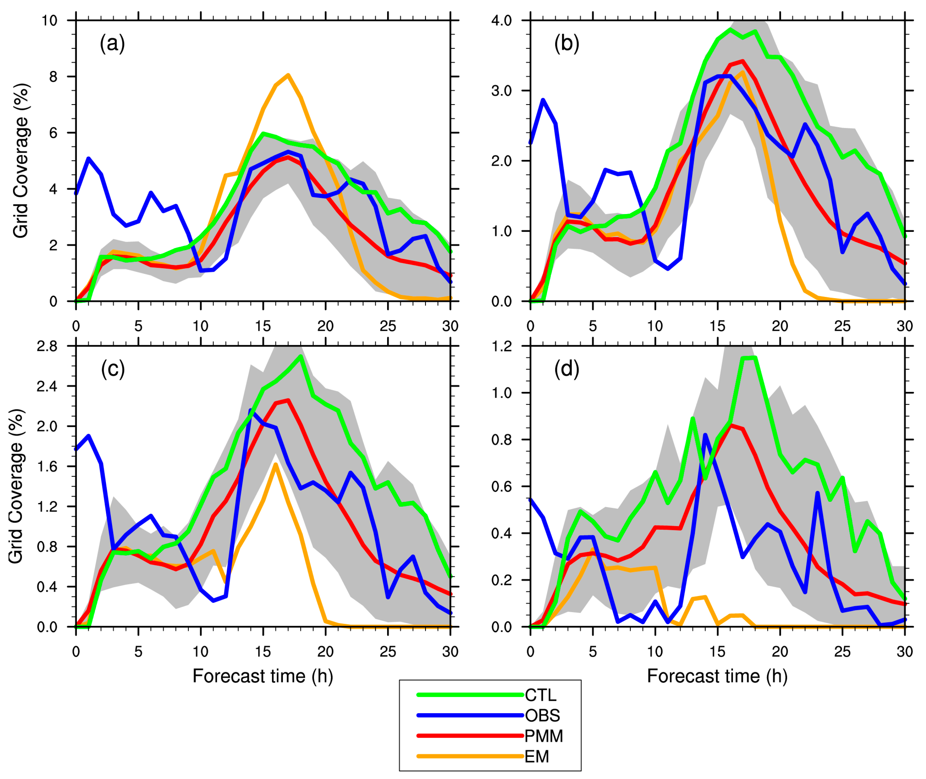
The evolution of grid coverages exceeding different rainfall thresholds over the forecast time is depicted in Figure 4, which reflects the ability to forecast different levels of precipitation. When the precipitation exceeded 1.0 mm/h (Figure 4a), the grid coverage produced by the PMM method was closer to the observations in terms of both the sizes and trends of the values. However, the grid coverages of the control forecast and EM method were higher than observed. When the precipitation exceeded 5.0 mm/h (Figure 4b), the grid coverages of the EM and PMM methods were similar to the observation values regarding both precipitation quantity and tendency, but the result for the control forecast was still higher. When the rainfall thresholds were 10.0 mm/h and 16.0 mm/h (Figure 4c,d), the grid coverages produced by the EM method were significantly reduced after the rainfall enhancement (after the 13th h), and decreased with an increasing rainfall threshold. At the level of rainstorms (q = 16.0 mm/h) the grid coverage produced by the EM method gradually became zero in the precipitation period, suggesting that the traditional EM method had poor forecasting capability for heavy rain. At the same time, the result for the control forecast was still higher, while the PMM method was closer to the observations. In general, the grid coverages of the EM method were better than those for the control forecast. The EM method had a better forecasting capability for the middle level of precipitation. The PMM method had the closest forecast result to the actual observed value at high magnitudes of precipitation. Therefore, in heavy precipitation cases, the PMM method should be applied to process the ensemble members, thus the limitation of the traditional EM method for predicting extreme precipitation could be remedied.
5. The Probabilistic Forecast Results
5.1. The Results of Spatial Neighborhood
5.1.1. Distribution of Spatial Neighborhood Probability
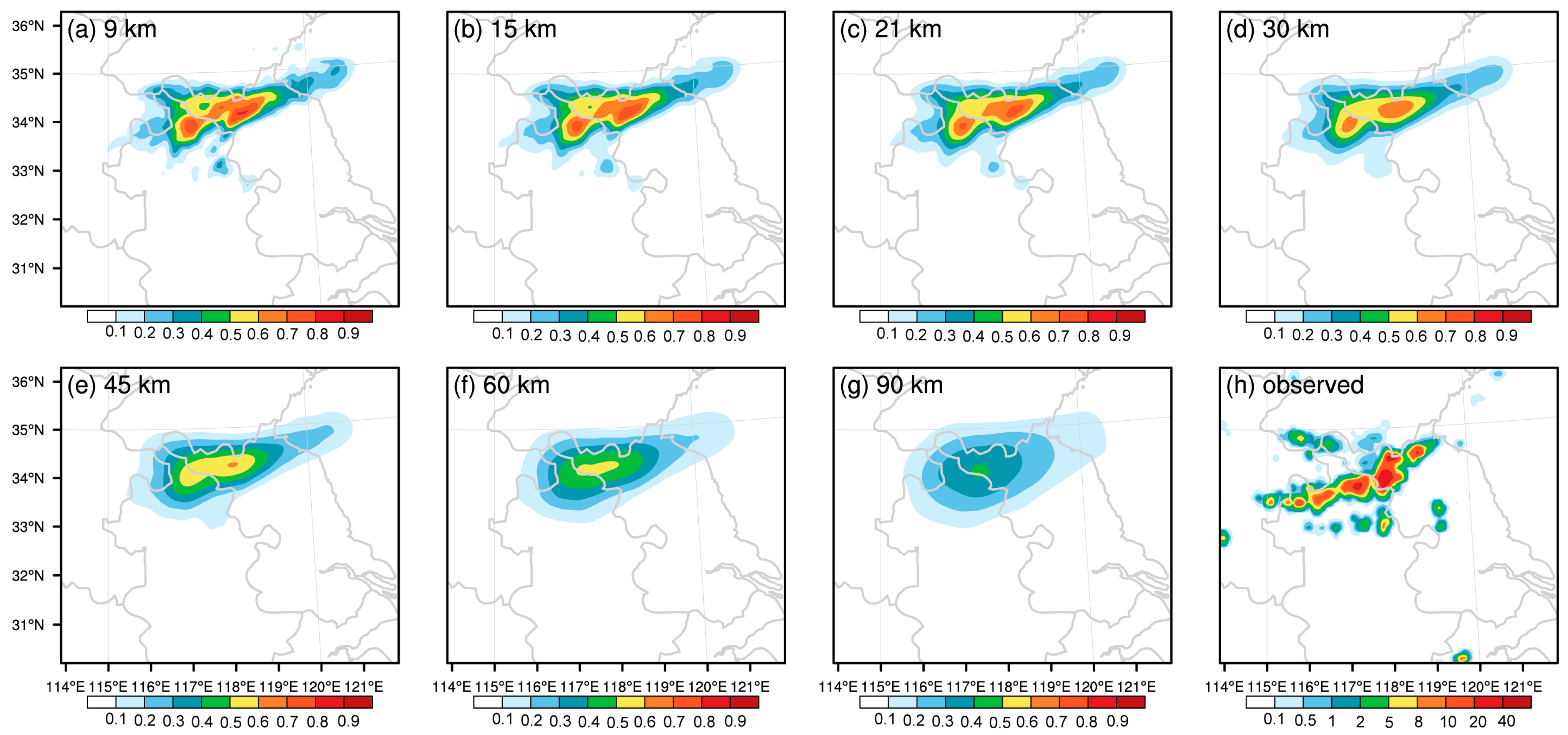
To demonstrate the characteristics of the NP products, Figure 5a–g shows the NP distribution at the time of the heaviest precipitation (14th h) under different neighborhood radii produced by the NEP method, focusing on the 1.0 mm/h rainfall threshold. The observed precipitation distribution at 0800 UTC, 30 July (14th h), is correspondingly depicted in Figure 5h for comparison. It can be seen from Figure 5h that the precipitation was an east to west zonal distribution and heavy precipitation centers were located at the Suqian and Suzhou areas, indicating the basic situation of the squall line process. Compared to the observed precipitation distribution, the NP distributions could give guiding probabilistic forecast results. The NP distributions tended to be smoother as the neighborhood radius increased, yet the probabilistic values tended to be smaller. The reason is that with the increase of the neighborhood range, the region outside the convective precipitation may be taken into consideration. Therefore, it is an issue worth exploring to determine the manner in which to select the neighborhood radius of appropriate spatial scale in order to produce the most reasonable probabilistic forecast results. When the neighborhood radius was under 45 km (Figure 5a–d), the probabilistic forecast produced relatively accurate results for not only the probabilistic range of precipitation exceeding 1.0 mm/h, but also the corresponding locations of high probability centers and two observed precipitation cells, showing that the spatial scale of 45 km could synthesize the light rainfall information and provide an indication for the occurrence of heavy precipitation. When the neighborhood radius exceeded 45 km (Figure 5f,g), the probabilistic center could still give some guidance for the prediction of precipitation events despite the small precipitation probability.
5.1.2. FSS of Spatial Neighborhood
Due to the highly non-linear characteristics of convective-scale weather systems, there were local spatial differences in the high-resolution convective-scale precipitation forecasts. Thus, an objective verification method should be adopted to determine the extent to which the spatial scale can characterize the spatial differences of convective-scale weather systems and their convective precipitation.
Figure 6 depicts the evolution of FSS over different neighborhood radii in the strongest rainfall (14th h). The figure shows that at all the rainfall thresholds, FSS values increased as the neighborhood radius increased, then slowed down at the radius of 45 km, and almost remained the same, indicating that the spatial scale of 45 km basically contained the local-scale information of such convective-scale weather systems. However, a larger spatial scale resulted in an artificial reduction of spatial resolution, and smoothed out some small-scale information, which was unable to meet the refinement requirements of the high-resolution convective-allowing ensemble forecast. At the rainstorm level, the FSS values reached their maximum at the neighborhood radius of 15–30 km (Figure 6d).
Furthermore, the FSS values tended to decrease with the increase of rainfall thresholds. When q = 1.0 mm/h (Figure 6a), the FSS of the NEP and PMM methods reached the highest, and the FSS of EM method was also obviously higher than that of the control forecast. When q = 5.0 mm/h (Figure 6b), the FSS value of the EM method was significantly reduced, while the FSS of the NEP method was still the highest. When q = 10.0 mm/h and q = 16.0 mm/h (Figure 6c,d), the FSSs of the PMM and NEP methods were better than those of the control forecast. Noticeably, the FSS obtained by the EM method was very small, notably, the score for heavy rainfall was almost zero in Figure 6d, indicating that the traditional EM method had a poor capability for predicting extreme precipitation. Therefore, the FSS verifications of the PMM and NEP methods were superior to that of the control forecast. The EM method was better than the control forecast in the verification of light rainfall, but the worst at predicting extreme precipitation. In addition, it was shown from the shaded portion that ensemble members had a good predicting capability for precipitation. The forecast results of some members should be taken into consideration when analyzing the results of ensemble forecasts.
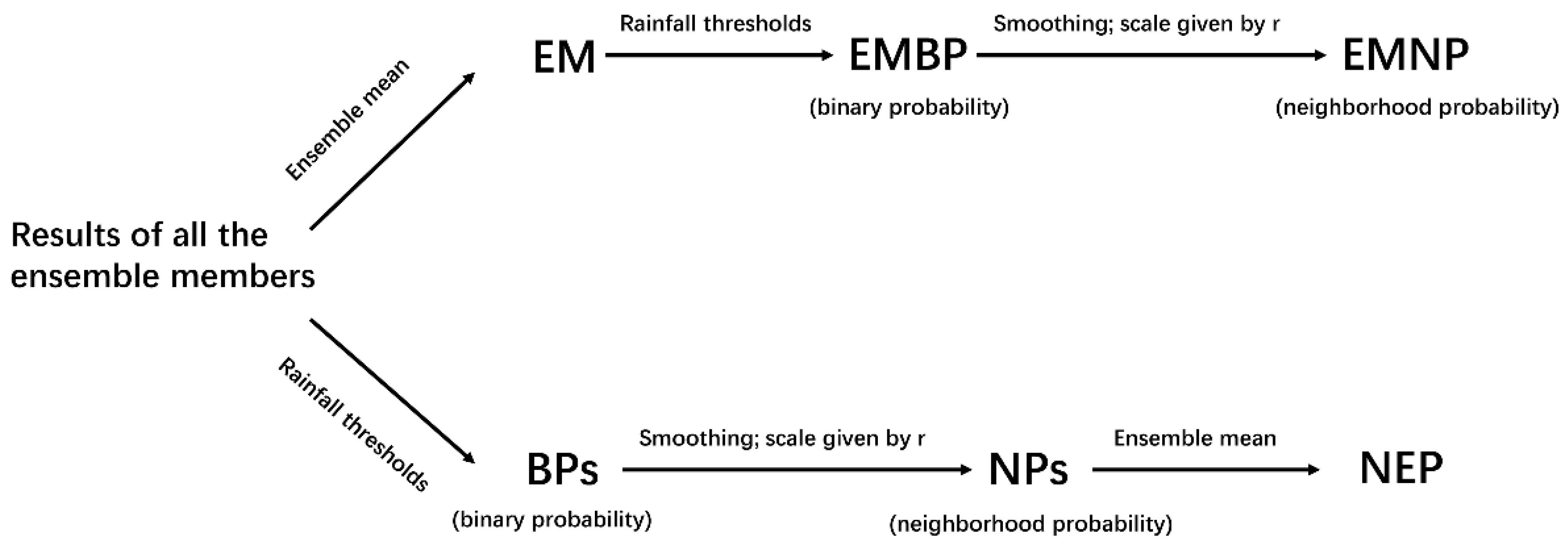
In particular, ensemble-mean neighborhood probability (EMNP) and neighborhood ensemble probability (NEP) differ only by the order of generation of the arithmetical averaging and the binary probability, whereas in Figure 6d, FSSs of NEP were much larger than those of EMNP. Regarding this phenomenon, a schematic diagram to generate EMNP and NEP was given to explain the possible causes of the phenomenon (Figure 7).
The EMNP is first averaged by the forecasting fields of all the ensemble members to obtain the EM field. Then, the EM field is calculated by Equation (1) to obtain the binary probability EM field (EMBP) at different rainfall thresholds. Finally, the EMBP is smoothed by different neighborhood radii to generate the EMNP. In the first step, the original precipitation information is simply averaged as a whole without distinguishing rainfall thresholds, which reduces the forecasting value for heavy precipitation. Therefore, the EMNP is generally small in heavy precipitation, which leads to a smaller FSS value in Figure 6c,d, especially with the score of heavy rainfall being almost zero. However, the NEP is first calculated by different rainfall thresholds to produce the binary probability fields of all the ensemble members (BPs). Next, the BPs are smoothed by different neighborhood radii to generate the NP of all the members (NPs). Lastly, the NPs are calculated by Equation (4) to get the NEP at different rainfall thresholds. Because NEP takes into full account the original information in heavy precipitation at the first step, the ensemble mean here is not as obvious as the smoothing effect of EMNP in heavy rainfall. As a result, NEP is larger than EMNP at the heavy rainfall threshold, resulting in much larger FSS values of the NEP method than those of the EM method.
However, the FSS values of the PMM method were similar to those of the NEP method in heavy precipitation. It is because the PMM method not only synthesizes the precipitation forecast values of all the ensemble members, but also highlights heavy rainfall information. Therefore, the PMM method has a higher forecasting skill for heavy precipitation.
5.1.3. ROC Curves of Spatial Neighborhood
ROC curves are used to evaluate the results of probabilistic forecasts at a certain rainfall threshold, reflecting the relationship between the probability of detection (POD) and the probability of false detection (POFD). When the forecast results are verified by the corresponding observed results, they are divided into four events in Table 2. The event of a hit is marked as a, the event of a false alarm is marked as b, the event of a missing forecast is marked as c, and the event that does not occur and is not forecast is marked as d. Then, the probability of detection (POD = a/(a + b)) and the probability of false detection (POFD = b/(b + d)) are calculated for each probabilistic threshold (thresholds of 0 to 100%, at 5% intervals). The ROC curve is formed by plotting the POFD against the POD over the range of probabilistic thresholds [15,20]. When the ROC curve is above the diagonal, it indicates a positive forecasting technique. In contrast, when the curve is below the diagonal, it indicates no forecasting skill.
Figure 8 shows the ROC curves exceeding 1.0 and 16.0 mm/h at the time of heaviest precipitation (14th h). As shown in Figure 8a, all dashed lines (45 km) were above the solid lines (15 km) of the corresponding color. The probabilistic forecast using the EM method performed the best in terms of predicting light rainfall events, and probabilistic forecasting skills of the 45 km spatial neighborhood were better than that of the 15 km neighborhood. For extreme precipitation (Figure 8b), the forecasting skills of the PMM and NEP methods were superior to those of EM and control forecast, and the spatial neighborhood of 15 km was more skillful than the 45 km spatial neighborhood. The results further confirmed that for the precipitation at different thresholds, the neighborhood radius that matches their spatial scales should be selected to generate a more reasonable probabilistic forecast.
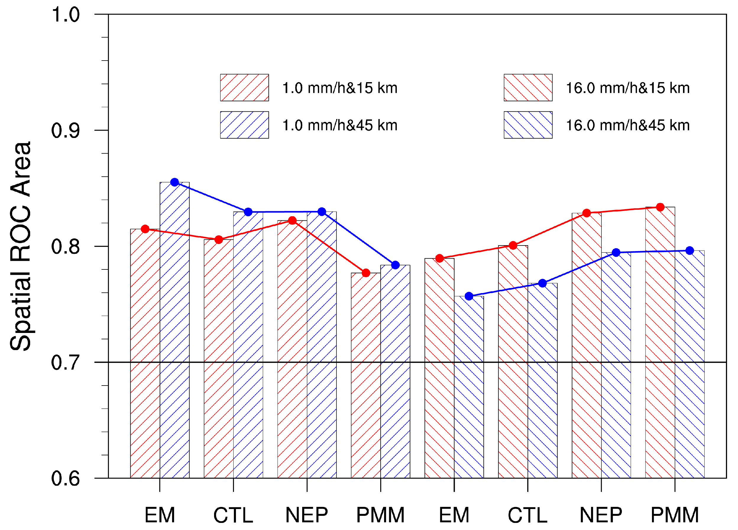
The area under this curve is the ROC area, and forecasting systems with a ROC area greater than 0.7 are considered useful [29]. The ROC areas in Figure 9 clearly showed that for light rainfall, the polyline of the 45 km neighborhood was above the polyline of the 15 km neighborhood. While the result of heavy precipitation was the opposite, in that the polyline of the 15 km neighborhood was above the polyline of the 45 km neighborhood, indicating that the spatial neighborhood of 15 km was more skillful than the 45 km neighborhood. Using a ROC area of 0.7 as a threshold to determine forecast effect, all neighborhood probability results could produce useful forecasts. Meanwhile, the NEP results of different rainfall thresholds all had higher forecasting skills.
5.2. The Results of Temporal Neighborhood
5.2.1. FSS of Temporal Neighborhood Included
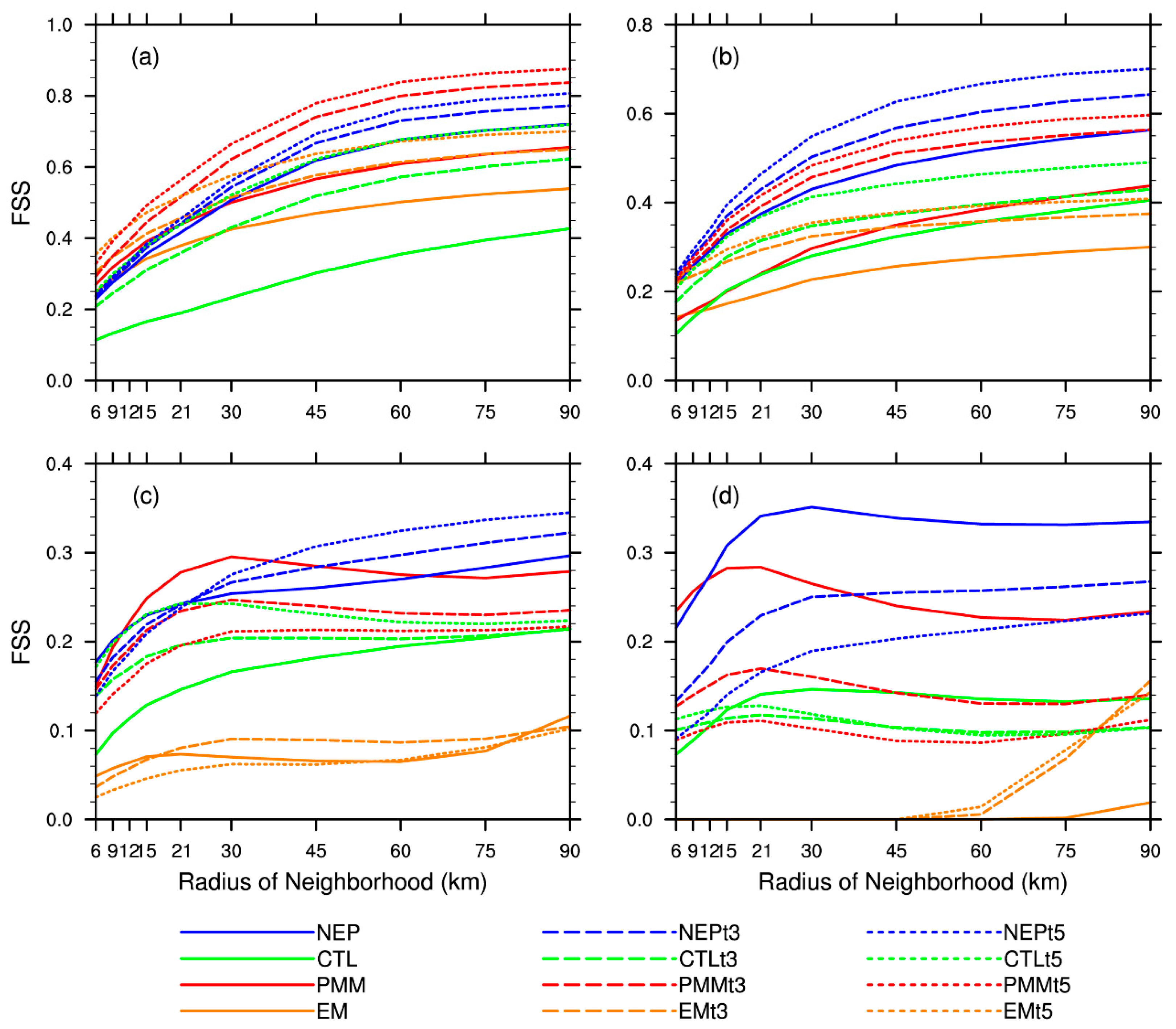
Figure 10 shows the FSS evolution of three temporal neighborhoods over the radius of the neighborhood. It could be seen that the FSS evolution with respect to spatial scale was basically consistent with the previous section. The focus of this section is the comparison of the influences of different temporal neighborhoods to the FSS, and the discussion of the temporal scales that can characterize the temporal differences of convective-scale weather systems and their convective precipitation.
When q = 1.0 mm/h and q = 5.0 mm/h (Figure 10a,b), the FSS values increased with the increasing temporal scale, suggesting that if we take temporal uncertainty out of consideration, the forecast capability for light rainfall would be underestimated. When q = 10.0 mm/h (Figure 10c), the FSS values of the EM method manifested as 3 h > 1 h > 5 h of temporal neighborhood, and the FSS of the PMM method as 1 h > 3 h > 5 h (i.e., the FSS was increasing as the temporal scale decreased). As the threshold increased to 16.0 mm/h (Figure 10d), compared to 10.0 mm/h, the temporal scale at 1 h was far larger than that of 3 h and 5 h by the PMM method (i.e., the FSS was increasing faster as the temporal scale decreased). The FSSs of the NEP method and control forecast were also increasing as the temporal scale decreased.
Therefore, for the light rainfall forecast, the larger the temporal scale, the larger the FSS value. With the increase of rainfall threshold, the FSS value of the 3 h temporal scale was larger than that of 1 h and 5 h. With a further increase of the rainfall threshold, the smaller the temporal scale, the larger the FSS value. This was because the 5 h temporal scale contained the uncertainty of light rainfall in convective-scale precipitation events. As the rainfall threshold increased, the temporal distribution of precipitation was also more concentrated, thus the corresponding temporal scale decreased as well. When the precipitation reached rainstorm level, a smaller temporal scale could reduce the temporal difference of precipitation so as to produce a better forecast effect. In this study, the minimum temporal scale was 1 h, reaching the largest FSS value in heavy rainfall. If the temporal resolution could increase to the minute level, a smaller temporal scale would be obtained and thus a larger FSS value would be obtained for the rainstorm.
5.2.2. Distribution of Temporal Neighborhood Probability
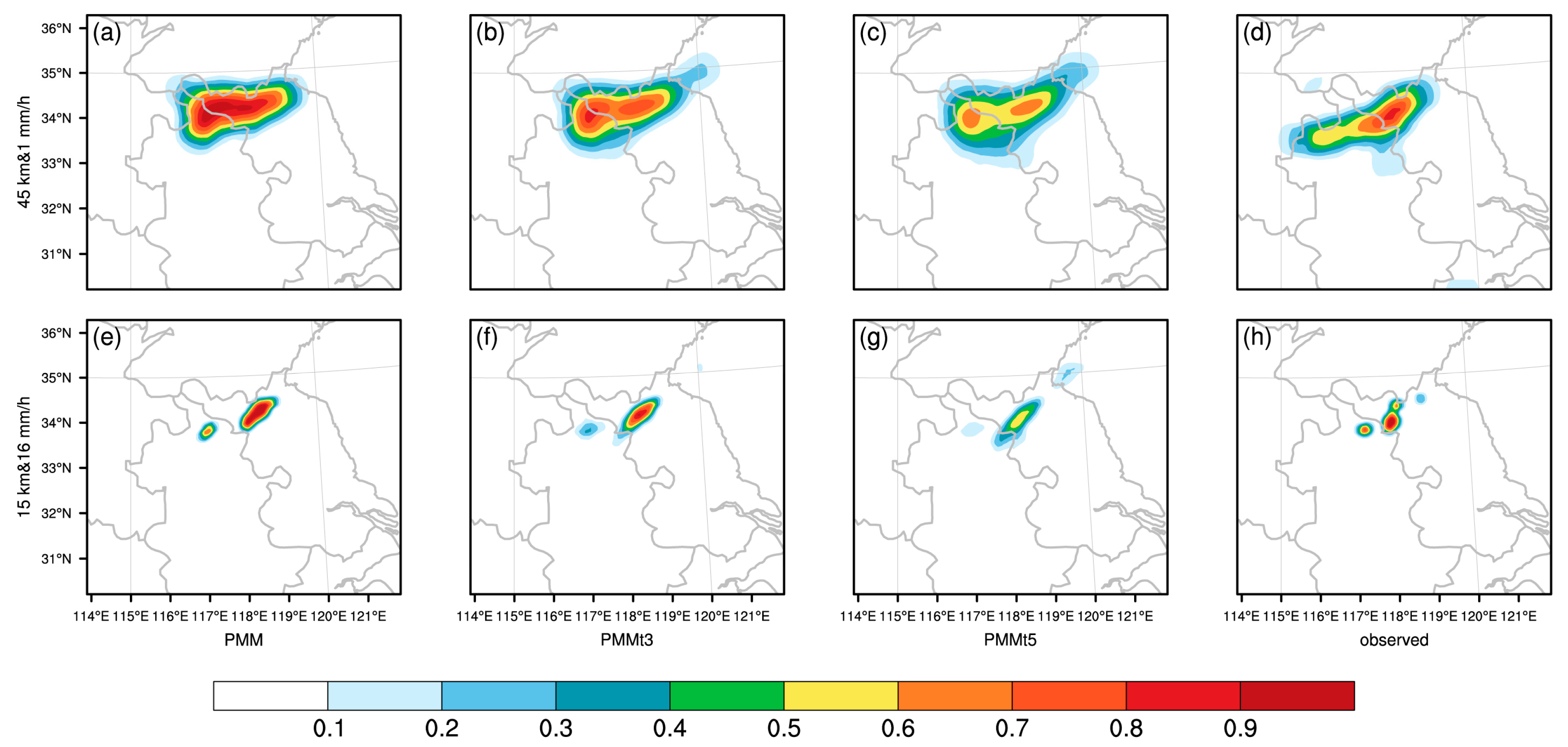
Selecting the representative combinations of 45 km and 1.0 mm/h and 15 km and 16.0 mm/h, the distributions of temporal neighborhood probability obtained by the PMM method, which had the most prominent changes of FSS in the different temporal neighborhoods, were taken as an example to reveal the influence of different temporal scales on probabilistic forecast results by comparing the observed and neighborhood probabilistic precipitation. The comparison of the heaviest rainfall (14th h) is shown in Figure 11.
With a 1.0 mm/h rainfall threshold and 45 km spatial scale, the NP distributions were basically in line with the observations (Figure 11a–d). In contrast, the distribution patterns of 5 h and 3 h temporal scales were closer to the observations than those of 1 h. When the rainfall threshold was 16.0 mm/h and the neighborhood radius was 15 km (Figure 11e–h), which is classed as a rainstorm, it could be seen that the smaller the temporal scale was, the closer the probabilistic distribution and value were to the observation. This was in agreement with the analysis in Section 5.2.1. The conclusion was also applicable to other times. Of course, when the location of forecasting precipitation systems matches that of the observed field, the improved NP method may produce better forecast results. However, when they do not match, the improved NP method may not be very helpful.
5.2.3. ROC Curves of Temporal Neighborhood
The ROC curves included in three temporal neighborhoods are shown in Figure 12. For the light rainfall, the probabilistic forecasting skill of 3 h and 5 h temporal neighborhoods were better than that of 1 h, and the forecasting skill of the 45 km spatial scale was better than the 15 km forecasting skill of all the temporal scales, as shown in Figure 12a. For heavy rainfall, the forecasting skill of the two spatial scales both increased with decreasing temporal scales, as seen in Figure 12b. This indicated that spatial neighborhood was more significant in light precipitation events, while temporal neighborhood was more influential in heavy rainfall events due to their short-lived nature.
Figure 13 shows the ROC areas from the curves in Figure 12, more intuitively showing that the forecasting skills of light rainfall increased with the increasing temporal scale, and the skills of heavy rainfall increased with the decrease of temporal scale. However, the use of the 5-h temporal scale, where the ROC areas were less than 0.7, could not produce useful forecast for heavy rainfall. This further indicated that temporal neighborhood was more sensitive to heavy precipitation events.
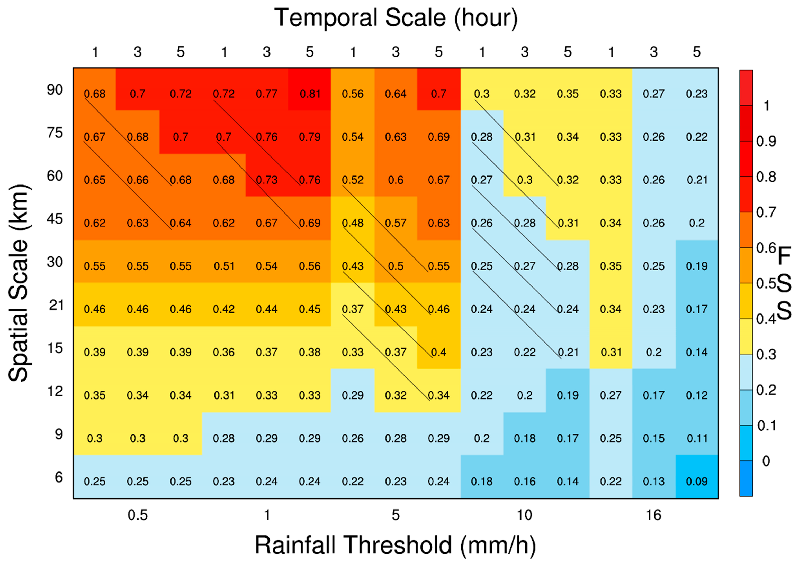
5.3. Comprehensive FSS of Spatial-Temporal Scales
The above two sections have considered the influence of spatial and temporal differences respectively on high-resolution convective-scale precipitation. In this section, the temporal scale is introduced into a threshold-scale diagram of FSS to explore the overall forecast effects of spatial-temporal neighborhoods. Figure 14 shows this threshold-scale diagram with temporal scales using FSSs of the NEP method at the 14th h. The conclusion could be drawn more directly that the FSS varied with rainfall thresholds, and spatial and temporal scales, respectively. Meanwhile, the spatial scale of 15–30 km neighborhood radius resulted in the highest FSS score when q = 16.0 mm/h and the temporal scale was 1 hour, which is consistent with the result of the spatial-neighborhood analysis in Section 5.2.
Further analysis could prove the existence of FSS constant lines (typical ones were lined out in Figure 14) with an approximate slope of 15–30 km/4 h in the spatial-temporal planes. These constant lines illustrate that the FSS values of smaller spatial scales and larger temporal scales were almost equal to those of larger spatial scales and smaller temporal scales. For example, FSSs of 90 km and 1 h and 60 km and 5 h, 75 km and 1 h and 45 km and 5 h, 60 km and 1 h and 30 km and 5 h, 30 km and 1 h and 15 km and 5 h, were similar. This fact suggested that the two neighborhood factors of spatial and temporal scales were interrelated for the precipitation forecast effects. For forecasters, selecting the combination of spatial and temporal resolution at the constant line is helpful. For example, for light rainfall events, forecasters can choose the 45 km and 3–5 h combination. For heavy precipitation, they can choose 15–30 km and 1 h combinations. We will try to increase the temporal and spatial resolution in order to provide more accurate and concrete combinations for forecasters.
In the case of light rainfall, FSS constant lines were concentrated at a larger spatial-scale area with a slope of approximately 30 km/4 h. As the rainfall threshold increased, the constant lines also showed up in a smaller spatial-scale area with a slope of 15–30 km/4 h. However, when the rainfall threshold was increased to rainstorm level, the constant lines did not exist. This was because the temporal neighborhood considered for heavy precipitation was relatively smaller, yet the constant lines may correspond to a smaller temporal scale as well. This indicated that there was an intrinsic relationship between the rainfall intensity, spatial scale, and temporal scale. That is, the slope of FSS constant lines under different rainfall thresholds may be affected by the inherent spatial-temporal scales of convective-scale weather systems.
6. Discussion and Conclusions
This study conducted a convection-allowing ensemble forecast experiment combined with a strong squall line process, using the PMM method to focus on extreme precipitation. The temporal dimension was introduced into the NP method, and the probabilistic forecast field was produced by the improved NP method. The forecast results were assessed by FSS and ROC curves analysis of different spatial-temporal neighborhoods to confirm the appropriate spatial and temporal scales of optimized high-resolution convective precipitation forecasts. The conclusions are as follows:
(1) Whether in the deterministic forecast, probabilistic forecast, or verification, the forecasting accuracy of ensemble forecast is basically higher than that of control forecast, which could improve forecasting skills.
(2) The NEP method, based on all ensemble members, could consider the precipitation information in a comprehensive and reasonable way, discriminatively processing the original data according to different rainfall thresholds. The PMM method focused on the information of heavy precipitation, which made the FSS and ROC curves of the NEP and PMM methods higher than those of the EM method in extreme precipitation events. The limitation of the EM method in extreme precipitation was remedied by the other two methods.
(3) The spatial scale with a neighborhood radius of 15 to 45 km could effectively rectify the precipitation error, which is a visual representation of spatial uncertainty. The neighborhood radius of 15–30 km produced more accurate probabilistic forecast results for heavy precipitation events at a smaller spatial scale. For light rainfall, the forecast effect became better as the temporal scale grew. For heavy rainfall, the forecast capability was improved as the temporal scale decreased. There was a corresponding relationship between temporal scale and rainfall intensity, so the temporal uncertainty of different levels of precipitation could be captured by different temporal scales, and a better forecast was thus produced.
(4) The spatial neighborhood is more significant in light precipitation events, while the temporal neighborhood is more influential for heavy precipitation events due to the short-lived nature of heavy rainfall events. In the threshold-scale diagram there exists FSS constant lines. These suggest that the influences of spatial and temporal scales on the precipitation forecast effect were interdependent, and could possibly be affected by the intrinsic spatial-temporal scale of convective-scale weather systems.
(5) The improved NP method could reflect the spatial and temporal uncertainties of convective-scale precipitation forecasts by high-resolution model synchronically, providing results that match different levels of precipitation. The findings were highly instructive for improving the skill of convective-scale precipitation forecasts.
The introduction of the temporal dimension into the concept of neighborhood enabled a comprehensive assessment of convective-scale precipitation forecasts at spatial and temporal scales. However, this study only conducted a preliminary investigation of one case. In our future work, experiments combined with more cases will be conducted in order to test the applicability of the improved NP method to arrive at a more general conclusion.
Acknowledgments
Thanks to the NCEP and NMIC for providing the relevant data. This paper was sponsored by the National Natural Science Foundation of China (No. 41205073 and No. 41275012) and Natural Science Foundation of Nanjing Joint Center of Atmospheric Research (NJCAR2016MS02).
Author Contributions
The work was a collaboration among all authors. Chaohui Chen designed the experiments and outlined the methods used. Shenjia Ma and Dan Wu performed the experiments and wrote the manuscript. Hongrang He and Chenxi Zhang modified the manuscript.
Conflicts of Interest
The authors declare no conflict of interest.
References
- Tennant, W. Improving initial condition perturbations for MOGREPS-UK. Q. J. R. Meteorol. Soc. 2015, 141, 2324–2336. [Google Scholar] [CrossRef]
- Bentzien, S.; Friederichs, P. Generating and calibrating probabilistic quantitative precipitation forecasts from the high-resolution NWP model COSMO-DE. Weather Forecast. 2012, 27, 988–1002. [Google Scholar] [CrossRef]
- Kühnlein, C.; Keil, C.; Craig, G.C.; Gebhardt, C. The impact of downscaled initial condition perturbations on convective-scale ensemble forecasts of precipitation. Q. J. R. Meteorol. Soc. 2014, 140, 1552–1562. [Google Scholar] [CrossRef]
- Schwartz, C.S.; Romine, G.S.; Weisman, M.L.; Sobash, R.A.; Fossell, K.R.; Manning, K.W.; Trier, S.B. A Real-Time Convection-Allowing Ensemble Prediction System Initialized by Mesoscale Ensemble Kalman Filter Analyses. Weather Forecast. 2015, 30, 1158–1181. [Google Scholar] [CrossRef]
- Schwartz, C.S.; Romine, G.S.; Sobash, R.A.; Fossell, K.R.; Weisman, M.L. NCAR’s Experimental Real-Time Convection-Allowing Ensemble Prediction System. Weather Forecast. 2015, 30, 1645–1654. [Google Scholar] [CrossRef]
- Xue, M.; Kong, F.; Weber, D.; Thomas, K.W.; Wang, Y.; Brewster, K.; Droegemeier, K.K.; Kain, J.S.; Weiss, S.J.; Bright, D.R.; et al. CAPS Realtime Storm-scale Ensemble and High-resolution Forecasts as Part of the NOAA Hazardous Weather Testbed 2007 Spring Experiment. In Proceedings of the 22th Conference on Weather Analysis and Forecasting, 18th Conference on Numerical Weather Prediction, Park City, UT, USA, 25–29 June 2007. [Google Scholar]
- Kong, F.; Xue, M.; Thomas, K.W.; Droegemeier, K.K.; Wang, Y.H.; Brewster, K.; Gao, J.D. Real-time storm-scale ensemble forecast experiment—Analysis of 2008 spring experiment data. In Proceedings of the 24th Conference on Several Local Storms, Savannah, GA, USA, 27–31 October 2008. [Google Scholar]
- Kong, F.; Xue, M.; Thomas, K.W.; Wang, Y.H.; Brewster, K.; Gao, J.D.; Droegemeier, K.K. A realtime storm-scale ensemble forecast system: 2009 spring experiment. In Proceedings of the 23th Conference on Weather Analysis and Forecasting, 19th Conference on Numerical Weather Prediction, Omaha, NE, USA, 1–5 June 2009. [Google Scholar]
- Xue, M.; Kong, F.; Thomas, K.W.; Wang, Y.H.; Brewster, K.; Gao, J.D.; Wang, X.G.; Weiss, S. CAPS Realtime Storm Scale Ensemble and High Resolution Forecasts for the NOAA Hazardous Weather Testbed 2010 Spring Experiment. In Proceedings of the 25th Conference on Several Local Storms, Denver, CO, USA, 11–14 October 2010. [Google Scholar]
- Clark, A.J.; Weiss, S.J.; Kain, J.S.; Jirak, I.L.; Coniglio, M.; Melick, C.J. An Overview of the 2010 Hazardous Weather Testbed Experimental Forecast Program Spring Experiment. Bull. Am. Meteorol. Soc. 2012, 93, 55–74. [Google Scholar] [CrossRef]
- Li, X.; He, H.; Chen, C.; Miao, Z.; Bai, S. A Convection-allowing ensemble forecast based on the breeding growth method and associated optimization of precipitation forecast. J. Meteorol. Res. 2017, 31, 955–964. [Google Scholar] [CrossRef]
- Zhuang, X.R.; Min, J.Z.; Wang, S.Z.; Zhou, K.; Cai, Y.C. A blending method for storm-scale ensemble forecast and its application to Beijing extreme precipitation event on July 21, 2012. Chin. J. Atmos. Sci. 2017, 41, 30–42. [Google Scholar] [CrossRef]
- Cai, Y.C.; Min, J.Z.; Zhuang, X.R. Comparison of different stochastic physics perturbation schemes on a storm-scale ensemble forecast in a heavy rain event. Plateau Meteorol. 2017, 36, 407–423. [Google Scholar] [CrossRef]
- Baldwin, M.E.; Kain, J.S. Sensitivity of Several Performance Measures to Displacement Error, Bias, and Event Frequency. Weather Forecast. 2006, 21, 636–648. [Google Scholar] [CrossRef]
- Schwartz, C.S.; Kain, J.S.; Weiss, S.J.; Xue, M.; Bright, D.R.; Kong, F.Y.; Thomas, K.W.; Levit, J.J.; Coniglio, M.C.; Wandishin, M.S. Toward Improved Convection-Allowing Ensembles: Model Physics Sensitivities and Optimizing Probabilistic Guidance with Small Ensemble Membership. Weather Forecast. 2010, 25, 263–280. [Google Scholar] [CrossRef]
- Mittermaier, M.P.; Roberts, N.M. Intercomparison of Spatial Forecast Verification Methods: Identifying Skillful Spatial Scales Using the Fractions Skill Score. Weather Forecast. 2010, 25, 343–354. [Google Scholar] [CrossRef]
- Ebert, E.E. Fuzzy verification of high-resolution gridded forecasts: A review and proposed framework. Meteorol. Appl. 2008, 15, 51–64. [Google Scholar] [CrossRef]
- Roberts, N.M.; Lean, H.W. Scale-Selective Verification of Rainfall Accumulations from High-Resolution Forecasts of Convective Events. Mon. Weather Rev. 2008, 136, 78–97. [Google Scholar] [CrossRef]
- Weusthoff, T.; Ament, F.; Arpagaus, M.; Rotach, M.W. Assessing the Benefits of Convection-Permitting Models by Neighborhood Verification: Examples from MAP D-PHASE. Mon. Weather Rev. 2010, 138, 3418–3433. [Google Scholar] [CrossRef]
- Clark, A.J.; Kain, J.S.; Stensrud, D.J.; Xue, M.; Kong, F.Y.; Coniglio, M.C.; Thomas, K.W.; Wang, Y.H.; Brewster, K.; Gao, J.D.; et al. Probabilistic Precipitation Forecast Skill as a Function of Ensemble Size and Spatial Scale in a Convection-Allowing Ensemble. Mon. Weather Rev. 2011, 139, 1410–1418. [Google Scholar] [CrossRef]
- Pan, L.J.; Zhang, H.F.; Chen, X.T.; Wang, J.P.; Chen, F.J. Neighborhood-based precipitation forecasting capability analysis of high-resolution models. J. Trop. Meteorol. 2015, 31, 632–642. [Google Scholar] [CrossRef]
- Kong, F.Y.; Droegemeier, K.K.; Hickmon, N.L. Multiresolution Ensemble Forecasts of an Observed Tornadic Thunderstorm System. Part I: Comparsion of Coarse- and Fine-Grid Experiments. Mon. Weather Rev. 2006, 134, 807–833. [Google Scholar] [CrossRef]
- Clark, A.J.; Gallus, W.A.; Xue, M.; Kong, F.Y. A comparison of precipitation forecast skill between small convection-allowing and large convection-parameterizing ensembles. Weather Forecast. 2009, 24, 1121–1140. [Google Scholar] [CrossRef]
- Ebert, E.E. Ability of a Poor Man’s Ensemble to Predict the Probability and Distribution of Precipitation. Mon. Weather Rev. 2001, 129, 2461–2480. [Google Scholar] [CrossRef]
- Berenguer, M.; Surcel, M.; Zawadzki, I.; Xue, M.; Kong, F.Y. The Diurnal Cycle of Precipitation from Continental Radar Mosaics and Numerical Weather Prediction Models. Part II: Intercomparison among Numerical Models and with Nowcasting. Mon. Weather Rev. 2012, 140, 2689–2705. [Google Scholar] [CrossRef] [Green Version]
- Schwartz, C.S.; Romine, G.S.; Smith, K.R.; Weisman, M.L. Characterizing and Optimizing Precipitation Forecasts from a Convection-Permitting Ensemble Initialized by a Mesoscale Ensemble Kalman Filter. Weather Forecast. 2014, 29, 1295–1318. [Google Scholar] [CrossRef]
- Ebert, E.E. Neighborhood Verification: A Strategy for Rewarding Close Forecasts. Weather Forecast. 2009, 24, 1498–1510. [Google Scholar] [CrossRef]
- Schwartz, C.S.; Kain, J.S.; Weiss, S.J.; Xue, M.; Bright, D.R.; Kong, F.Y.; Thomas, K.W.; Levit, J.J.; Coniglio, M.C. Next-Day Convection-Allowing WRF Model Guidance: A Second Look at 2-km versus 4-km Grid Spacing. Mon. Weather Rev. 2009, 137, 3351–3372. [Google Scholar] [CrossRef]
- Stensrud, D.J.; Yussouf, N. Reliable Probabilistic Quantitative Precipitation Forecasts from a Short-Range Ensemble Forecasting System. Weather Forecast. 2007, 22, 3–17. [Google Scholar] [CrossRef]
Figure 1.
The Weather Research Forecasting (WRF) model domain settings.

Figure 2.
A schematic diagram of the neighborhood probability (NP) method. Precipitation exceeds the threshold in the shaded boxes and is marked as “1”, otherwise it is marked as “0” in white boxes, and a radius of 2.5 times the grid length is specified.
Figure 2.
A schematic diagram of the neighborhood probability (NP) method. Precipitation exceeds the threshold in the shaded boxes and is marked as “1”, otherwise it is marked as “0” in white boxes, and a radius of 2.5 times the grid length is specified.
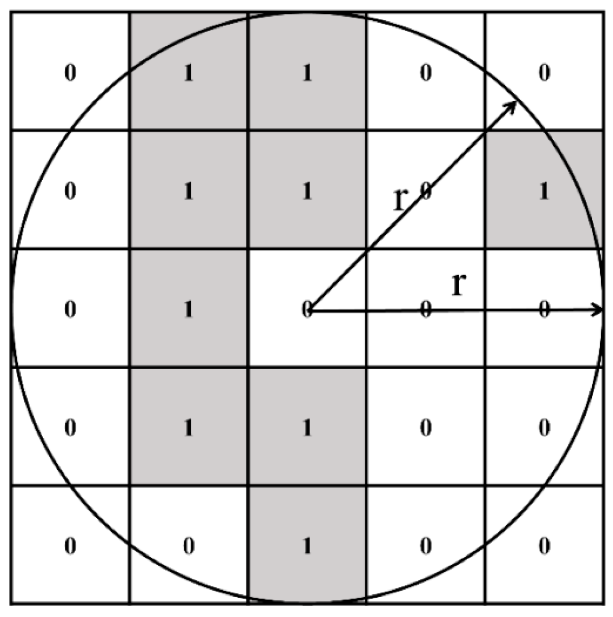
Figure 3.
The evolution of total hourly precipitation in domain 02 over the forecast time. The blue, orange, red, and green lines represent the observation (OBS), the ensemble mean (EM), the probability matched mean (PMM), and the control forecast (CTL), respectively. The shaded portion indicates the forecast range of all the ensemble members.
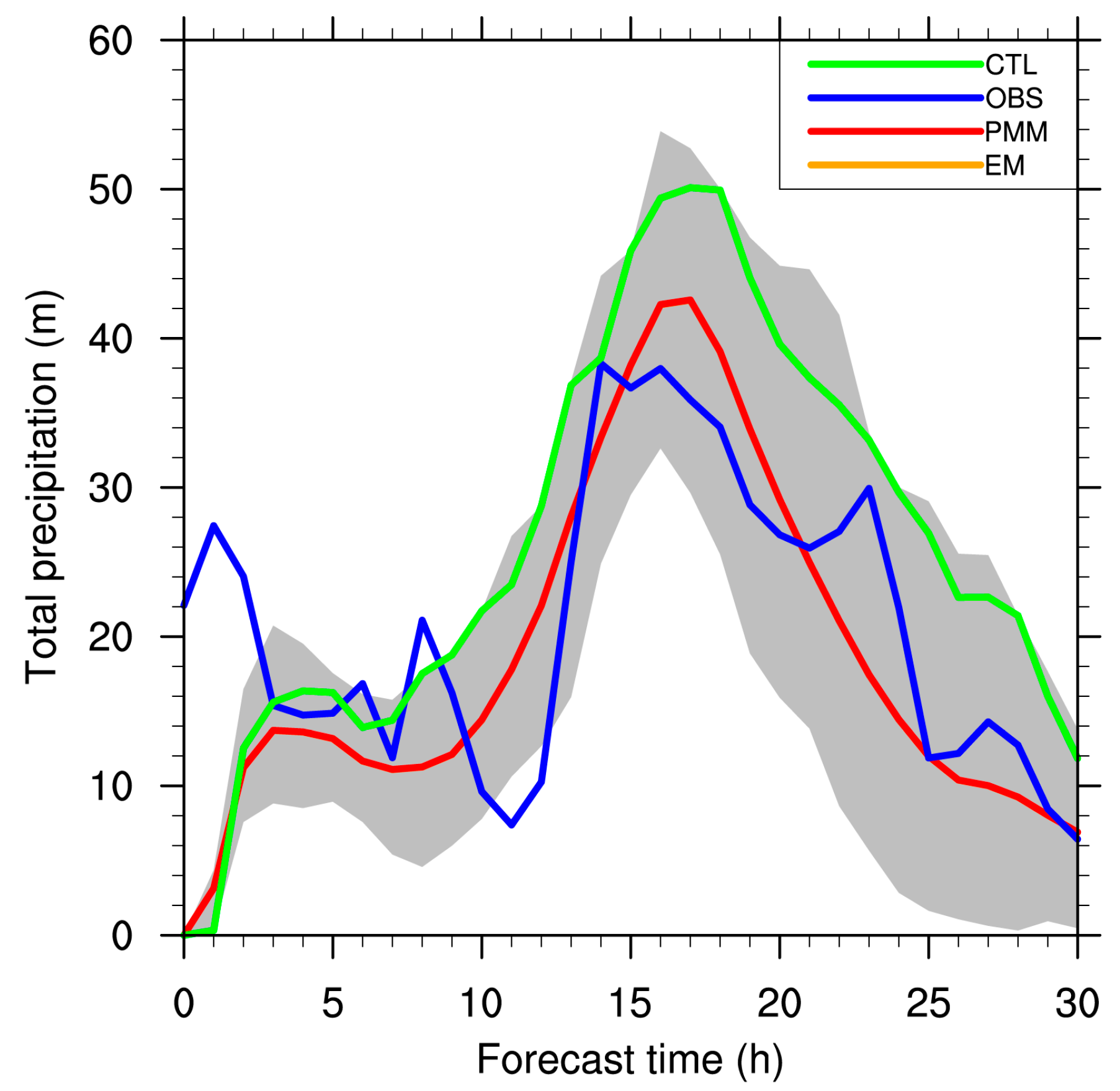
Figure 4.
The evolution of grid coverage of hourly precipitation exceeding (a) 1.0, (b) 5.0, (c) 10.0, and (d) 16.0 mm/h over the forecast time. The line descriptions are the same as in Figure 3.
Figure 4.
The evolution of grid coverage of hourly precipitation exceeding (a) 1.0, (b) 5.0, (c) 10.0, and (d) 16.0 mm/h over the forecast time. The line descriptions are the same as in Figure 3.

Figure 5.
The neighborhood ensemble probability distribution of precipitation exceeding 1.0 mm/h at the 14th h. The neighborhood radii (a–g) in turn are 9 km, 15 km, 21 km, 30 km, 45 km, 60 km, and 90 km, and panel (h) represents the observed precipitation distribution (units: mm).
Figure 5.
The neighborhood ensemble probability distribution of precipitation exceeding 1.0 mm/h at the 14th h. The neighborhood radii (a–g) in turn are 9 km, 15 km, 21 km, 30 km, 45 km, 60 km, and 90 km, and panel (h) represents the observed precipitation distribution (units: mm).

Figure 6.
The fractions skill score (FSS) of precipitation exceeding (a) 1.0, (b) 5.0, (c) 10.0, and (d) 16.0 mm/h at the 14th h over the radius of neighborhood. The green line is the control forecast (CTL), the blue, orange, and red lines represent neighborhood ensemble probability (NEP), EM, and PMM methods, respectively. The shaded portion indicates the forecast range of all the ensemble members.
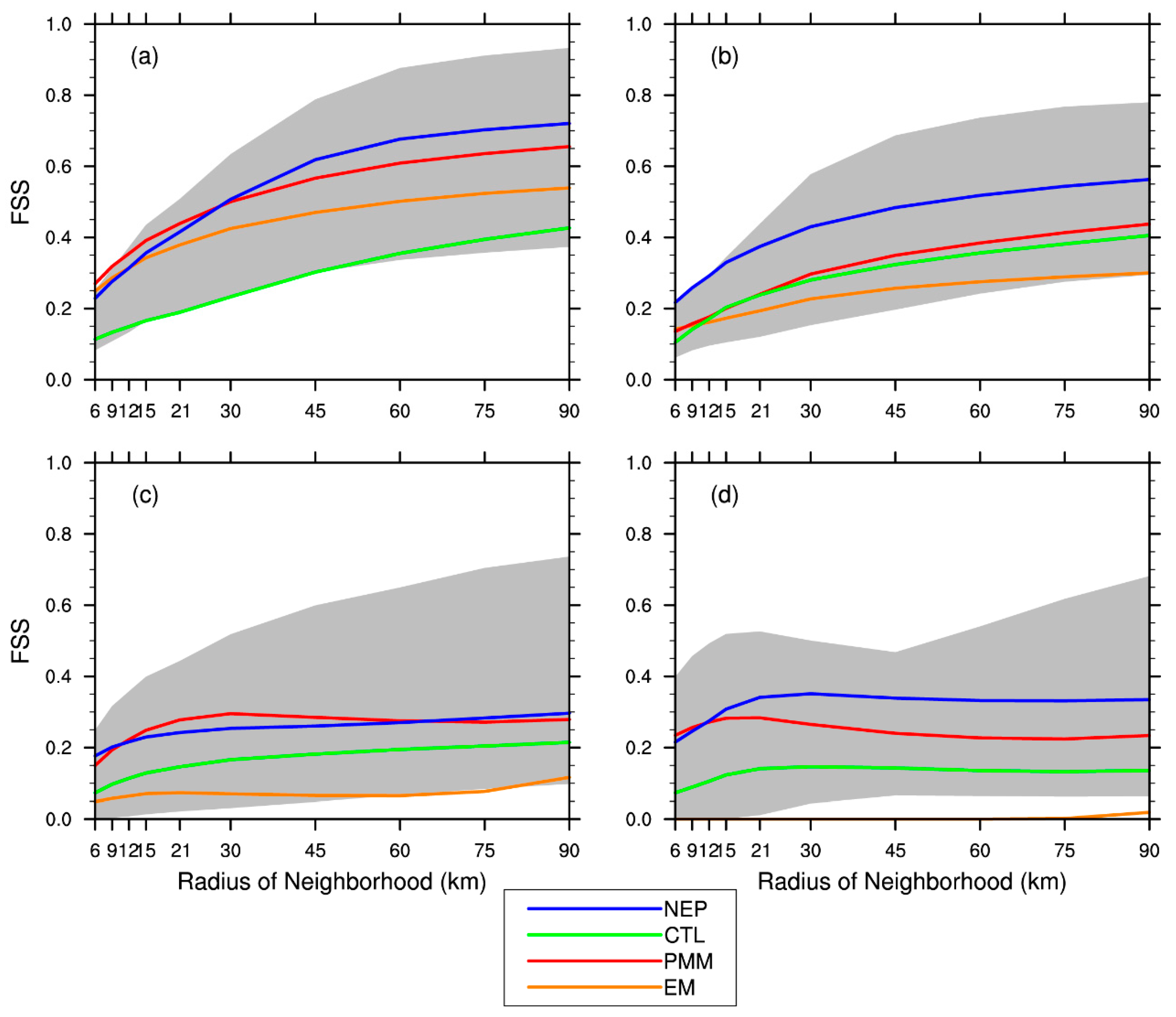
Figure 7.
The steps to generate ensemble-mean neighborhood probability (EMNP) and NEP. EMBP: binary probability EM field.
Figure 7.
The steps to generate ensemble-mean neighborhood probability (EMNP) and NEP. EMBP: binary probability EM field.

Figure 8.
Relative operating characteristic (ROC) diagrams of precipitation exceeding (a) 1.0 and (b) 16.0 mm/h at the 14th h. The solid and dashed lines represent the spatial neighborhood radius of 15 km and 45 km, respectively, and the colors are the same as in Figure 6. POD: probability of detection; POFD: probability of false detection.
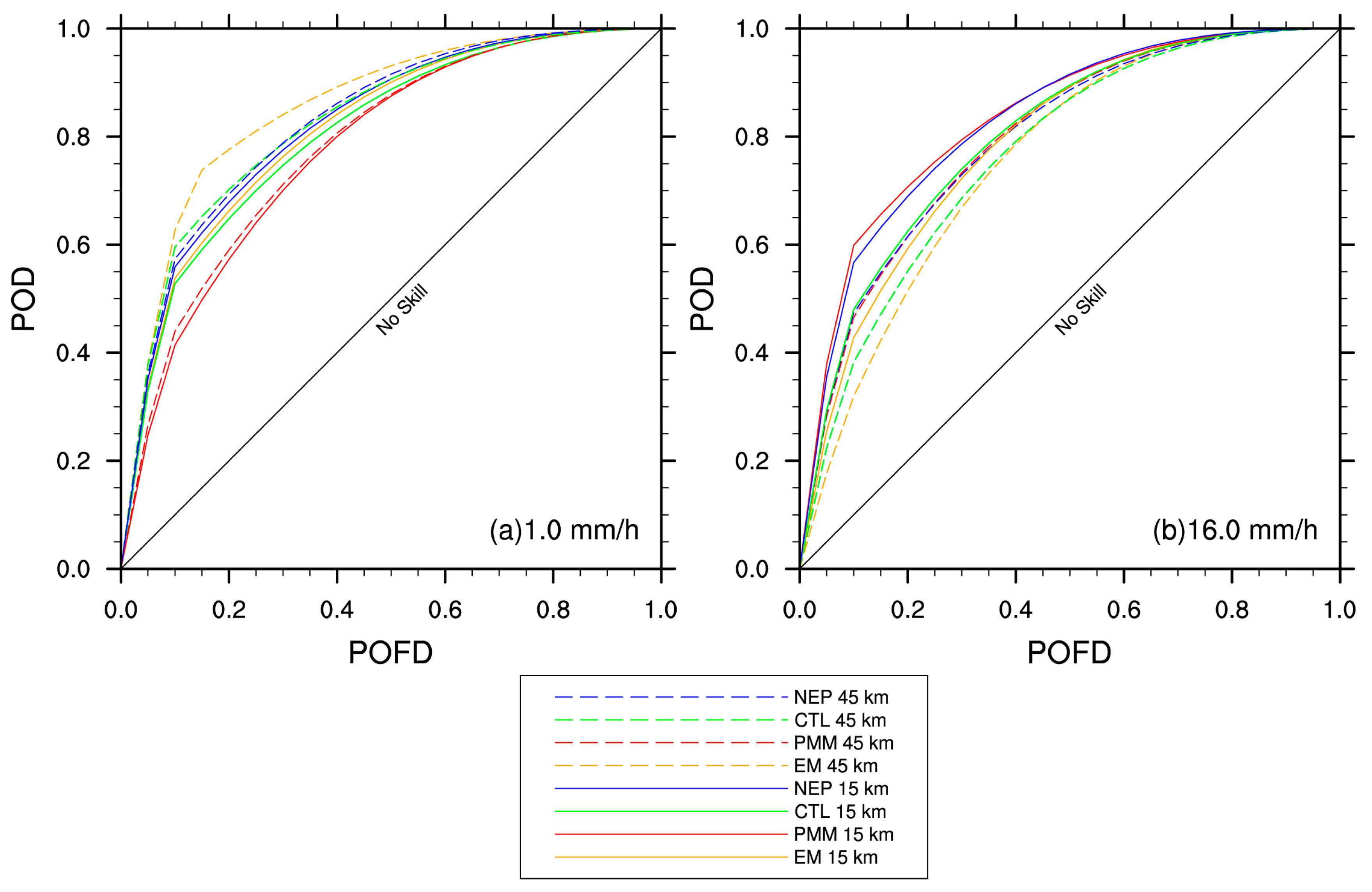
Figure 9.
The histogram superimposed polyline chart of the ROC areas from ROC curves in Figure 8. The red and blue lines represent the spatial neighborhood radius of 15 km and 45 km, respectively.
Figure 9.
The histogram superimposed polyline chart of the ROC areas from ROC curves in Figure 8. The red and blue lines represent the spatial neighborhood radius of 15 km and 45 km, respectively.

Figure 10.
Three temporal-neighborhood FSSs of precipitation exceeding (a) 1.0, (b) 5.0, (c) 10.0, and (d) 16.0 mm/h at the 14th h over the radius of neighborhood. The solid, long dashed, and short dashed lines represent 1 h, 3 h, and 5 h temporal neighborhoods, respectively, and the colors are the same as in Figure 6.

Figure 11.
The NP distribution of three temporal neighborhoods and observation at the 14th h. Panels (a–d) represent 1 h, 3 h, 5 h temporal neighborhood and observation using a radius of 45 km and exceeding 1.0 mm/h, respectively, and panels (e–h) represent using a radius of 15 km and exceeding 16.0 mm/h, respectively.

Figure 12.
ROC diagrams of precipitation exceeding (a) 1.0 and (b) 16.0 mm/h at the 14th h. The solid and dashed lines represent the 15 km and 45 km neighborhood radii, respectively, and the blue, red, and green lines represent 1 h, 3 h, and 5 h temporal neighborhoods, respectively.
Figure 12.
ROC diagrams of precipitation exceeding (a) 1.0 and (b) 16.0 mm/h at the 14th h. The solid and dashed lines represent the 15 km and 45 km neighborhood radii, respectively, and the blue, red, and green lines represent 1 h, 3 h, and 5 h temporal neighborhoods, respectively.
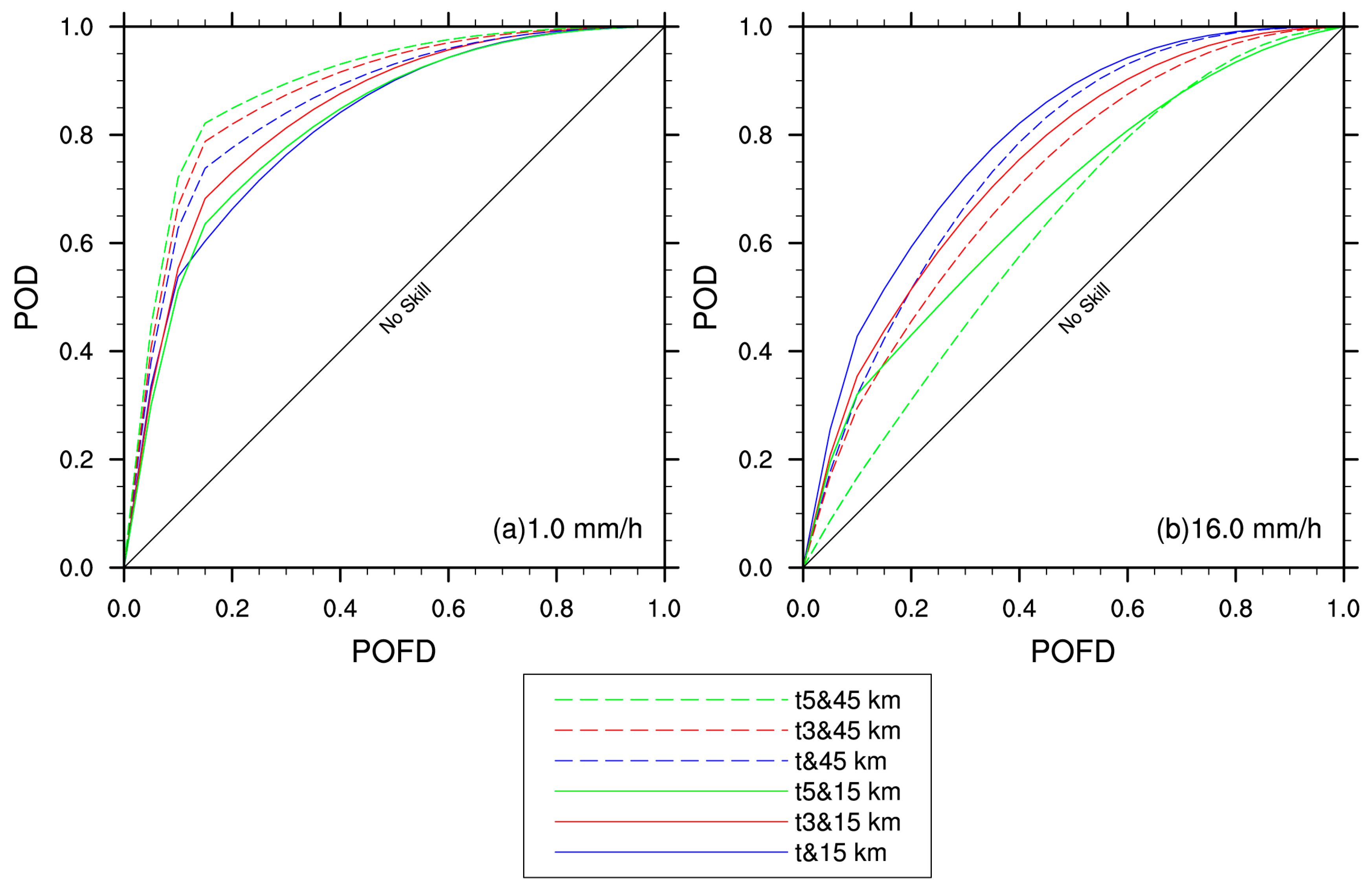
Figure 13.
Same as Figure 9, but the ROC areas from ROC curves in Figure 12. The red and blue lines represent the spatial neighborhood radius of 15 km and 45 km, respectively.
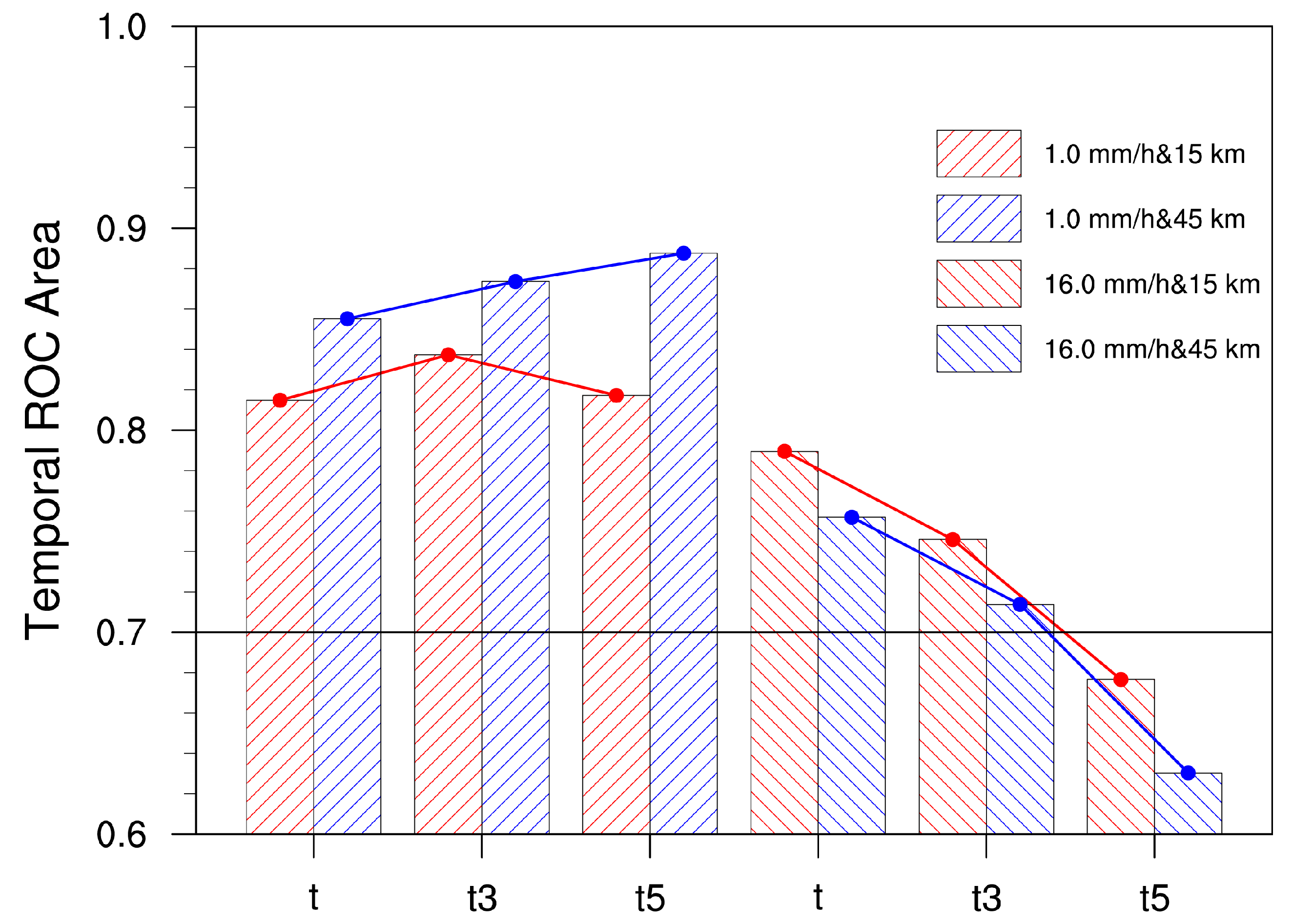
Figure 14.
Threshold-scale diagram with temporal scales at the 14th h. The bottom of the horizontal axis represents rainfall threshold, the top of the horizontal axis represents temporal scales corresponding to different rainfall thresholds, the vertical axis represents different spatial scales, and the value in each box is FSS. The diagonal lines represent FSS constant lines.


Table 1.
Basic physical parameterization settings.
| Physical Parameterization | Outer Domain (d01) | Inner Domain (d02) |
|---|---|---|
| Cumulus | Grell-Freitas scheme | None |
| Microphysics | Morrison double-moment scheme | |
| Longwave radiation | Rapid Radiative Transfer Model scheme (RRTM) | |
| Shortwave radiation | Dudhia scheme | |
| Planetary boundary layer | Yonsei University scheme | |
| Land surface | Noah land surface model | |
Table 2.
Standard 2 × 2 contingency table for dichotomous events.
| Observed | ||||
| Yes | No | |||
| Forecast | Yes | a | b | a + b |
| No | c | d | c + d | |
| a + c | b + d | |||
© 2018 by the authors. Licensee MDPI, Basel, Switzerland. This article is an open access article distributed under the terms and conditions of the Creative Commons Attribution (CC BY) license (http://creativecommons.org/licenses/by/4.0/).
Share and Cite
MDPI and ACS Style
Ma, S.; Chen, C.; He, H.; Wu, D.; Zhang, C. Assessing the Skill of Convection-Allowing Ensemble Forecasts of Precipitation by Optimization of Spatial-Temporal Neighborhoods. Atmosphere 2018, 9, 43. https://doi.org/10.3390/atmos9020043
AMA Style
Ma S, Chen C, He H, Wu D, Zhang C. Assessing the Skill of Convection-Allowing Ensemble Forecasts of Precipitation by Optimization of Spatial-Temporal Neighborhoods. Atmosphere. 2018; 9(2):43. https://doi.org/10.3390/atmos9020043
Chicago/Turabian StyleMa, Shenjia, Chaohui Chen, Hongrang He, Dan Wu, and Chenxi Zhang. 2018. "Assessing the Skill of Convection-Allowing Ensemble Forecasts of Precipitation by Optimization of Spatial-Temporal Neighborhoods" Atmosphere 9, no. 2: 43. https://doi.org/10.3390/atmos9020043
Note that from the first issue of 2016, this journal uses article numbers instead of page numbers. See further details here.