Megacity-Induced Mesoclimatic Effects in the Lower Atmosphere: A Modeling Study for Multiple Summers over Moscow, Russia

Abstract

Urbanization leads to distinct meteorological features of urban environments, and one the best-known is the urban heat island (UHI) effect. For megacities, these features become mesoscale phenomena (scale ≥ 10 km) that are amplified by the tropospheric feedbacks, and have substantial implications on human well-being. For the first time, a three-dimensional statistical description of the megacity-induced meteorological effects extending towards the lower troposphere for summer is acquired on a quasi-climatological timescale (a decade) based on high-resolution (1 km) simulations for Moscow with the COSMO-CLM model with and without its urban canopy model TERRA_URB. Our results confirm the features from previous observational and modeling studies, including the UHI itself, the cooling effect above established by the cross-over effect, the urban dry/moist islands and the urban breeze circulation. Particularly, the UHI shows a strong diurnal variation in terms of intensity and vertical extent between daytime (≈0.5 K/≈1.5 km) and nighttime (>3 K/≈150 m). We have discovered a systematic veering in the downwind shift of the UHI spatial pattern established by the Coriolis effect, and an enhanced stable stratification of the rural surroundings established by the urban plumes further downwind. Finally, extending the analysis to multiple summers demonstrates a substantial increase in summer precipitation (up to +25%) over the city center and its leeward side. These urban-caused mesoclimatic effects need to be taken into account in weather and climate services, including the design of future megacities.

1. Introduction

Essential features of urban climate are deviations of the temperature and humidity from surrounding rural environment, known as urban heat island (UHI) and urban dry/moisture islands (UDI/UMI). Investigation of these effects and taking them into account within the framework of different weather and climate services is especially important due to their significant environmental and social impacts. In general, such impacts are considered as negative due to urban-caused acceleration of climate warming in the cities [1,2,3] and amplification of the heat waves [4,5] and related heat stress [6,7] affecting the human health and even mortality rates [8,9,10]. The drivers of urban–rural temperature and humidity differences and their near-surface climatology are well-studied for a big variety of cities all over the world (see classic studies [11,12] and review papers [13,14]). UDI and UMI effects are described, e.g., in [15,16,17,18].

The micro-climatological features established by the local urban environment (street canyons, parks, etc.) are generally limited to the urban canopy itself spanning in the air up to the roof level. However, for medium-sized urban areas and megacities, influence of surface parameters that differ from surrounding rural areas (in terms of albedo, roughness, thermal structure, evaporative cooling, etc.) is accumulated over the whole urban area reaching spatial extent of tens of kilometers or even more. In turn, these distinct surface features result in meteorological features of temperature, humidity and wind speed at similar spatial scales. According to the classification of atmospheric processes by scale (e.g., [19]), such features can be considered as mesoscale phenomena.

These “urban-caused mesoclimatic phenomena” involve interactions with the troposphere aloft by changing the size and properties of the atmospheric boundary layer (ABL) [20] particularly leading to the “boundary-layer urban heat island” (e.g., [21,22]) and urban-induced mesoscale circulations [23,24,25]. They further affect other tropospheric features such as the presence of cumulonimbus clouds and convective precipitation [26,27,28] through the changes in the triggering of moist-convection [29]. The urban-caused mesoclimatic phenomena interacting with the troposphere play the key role in the climate of the entire urban agglomerations: they do not only involve the “bottom-up” urban forcing affecting the troposphere that scales with the city extent as described above, but also the “top-down” tropospheric feedbacks that further amplify the distinct climatic conditions in the urban canopy. Examples of the latter are the advection of hot air between urban neighborhoods resulting in an UHI intensification with city sizes [7,30,31], the down-mixing of hot air due to the cross-over effect [21,32,33], and cascade effects such as the changes in radiation and rain hitting the cities that lead to an additional modulation of the surface energy and water balance.

The number of studies devoted to urban-caused climate phenomena that consider the lower troposphere is much smaller than those focusing only on the near-surface climate features. This could be explained by three reasons: (1) interest in layer in which we live; (2) difficulties of making continuous observations above the roof level; and (3) significantly higher complexity of three-dimensional atmospheric processes in ABL and lower troposphere, especially for coastal and mountain cities.

As such, most existing studies considering the urban–tropospheric interactions listed above are based only on episodic observations (the case studies), which have the insufficient timespan for making conclusions on urban–climate statistics. Moreover, various urban-induced tropospheric effects are studied by different methods and for cities located in different climatic zones and terrain types, which makes the understanding of the overall picture especially difficult. Therefore, quantitative and even qualitative estimates of such urban effects vary strongly. For example, estimations of the vertical extent of the UHI over big cities vary from 100–300 m [21,22,34] to 1–2 km [1,33,35,36] in dependence from the day time and season. The estimates of climatological or seasonal means also vary significantly. Understanding of urban effects on precipitation [28], cloudiness and wind regime is even more complicated.

Recent developments in field of modeling of atmospheric dynamics and computation techniques have opened new opportunities to study these urban-induced mesoscale atmospheric processes and feedbacks with a high detail in a systematic way towards the climatological timescale. Modern limited-area atmospheric models are possible to simulate meteorological regime over wide areas (from hundreds to thousands of kilometers) with horizontal grid spacing of few kilometers and even less, which allows directly resolving most mesoscale processes. In addition, models allow running various sensitivity experiments for in depth investigation of urban–atmospheric interactions.

In this study, we consider the result of application of such modeling approach, based on numerical experiments with COSMO-CLM regional climate model, to study the urban-caused mesoclimatic features of Moscow megacity, which is the biggest monocentric agglomeration in Europe and a promising place for urban climate studies (see Section 2.1).

The aim of this paper is to investigate the influence of a big urban agglomeration on the meteorological regime of the lower troposphere in terms of the temperature, humidity, wind and precipitation within similar methodology and compare results with existing studies based on various observations. In contrast to several similar modeling studies, based on simulations for short periods (few days, e.g. [24,32]), we consider simulations conducted at a quasi-climatological time scale (a decade). Study is focused on summer due to: (1) higher probability of cases with anticyclonic weather and intensive UHI; (2) higher relevance of urban climate studies firstly because of urban-induced heat stress during heat waves [4,5,6]; and (3) existing problems for simulations winter-time meteorological regime within considered modeling framework [37].

2. Methods

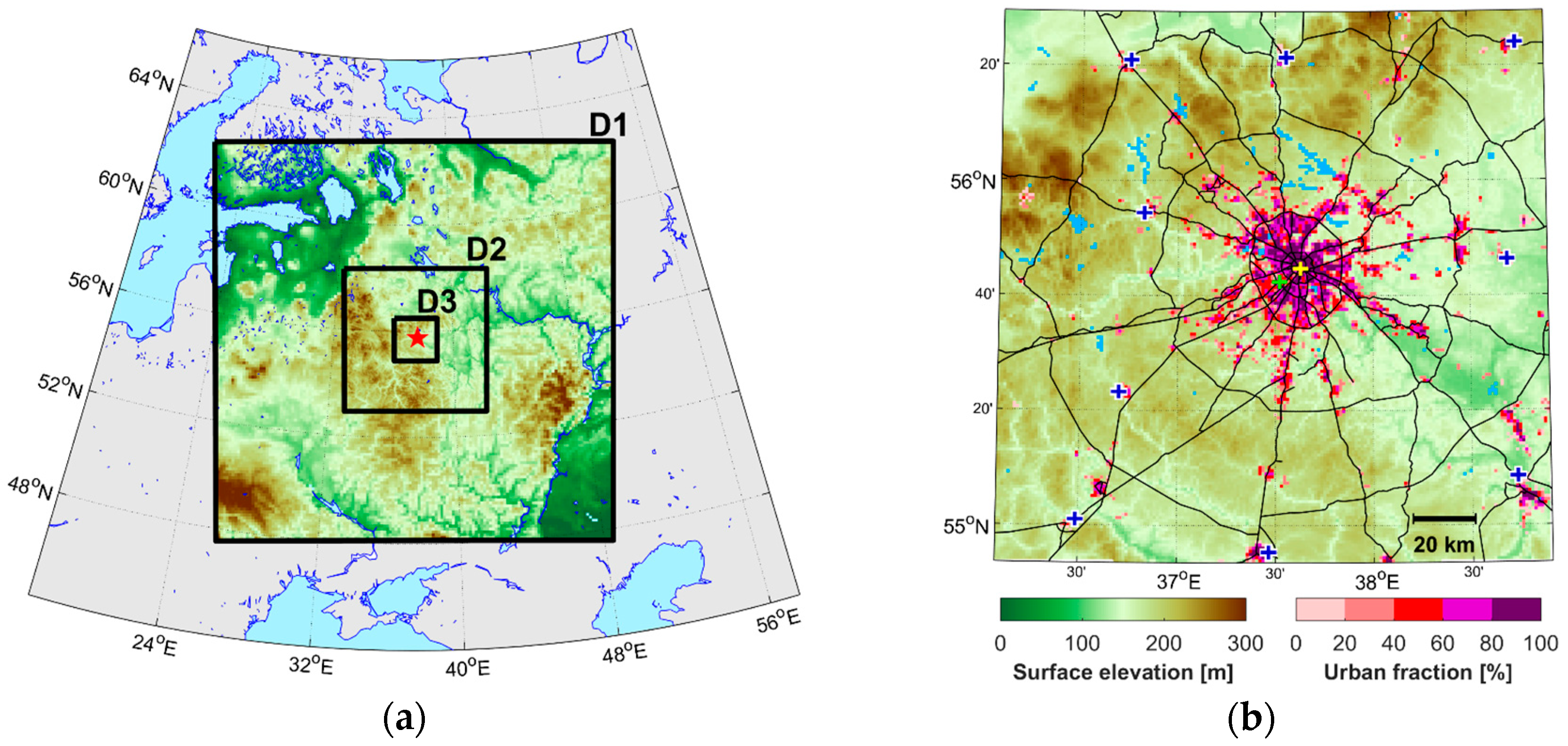
2.1. The Study Area

Moscow megacity is the biggest monocentric agglomeration in Europe. The population of the administrative unit is about 12 million people, while population of whole urban agglomeration is 16–17 million people [38]. The population of Moscow is rapidly increasing: since 1970, it has grown by more than 60%. The area of Moscow (the administrative unit) is ≈2500 km², however it includes a wide area known as “New Moscow”, which was joined to the city in 2011, but remains practically unbuilt. The actual area of the city (excluding the suburbs and satellite cities) is about 1000 km². Unlike most European and American cities, Moscow is densely built by the midrise and high-rise block-houses, while private low-rise houses are practically absent. According to the classification of Stewart and Oke [39], the prevailing types of local climate zones in Moscow are 2 (compact midrise), 4 (open high-rise) and 5 (open midrise) [40].

The Köppen Climate Classification subtype for Moscow is “Dfb” (Warm Summer Continental Climate). The mean annual rural temperature (according to observations at nine rural stations, see Figure 1) for recent WMO standard period (1981–2010) is 5.1 °C, mean summer (JJA) temperature is 17.2 °C and mean winter (DJF) temperature is −7.2 °C. The mean annual precipitation amount is about 700 mm [41] with a typical summer maximum. Due to the size and listed climate and building features, Moscow forms an intensive UHI with a mean annual intensity value equal to 2 K (for Balchug weather station at the city center, see Figure 1) and its maximum values up to 12–13 K [41]. Such values of mean annual UHI intensity are higher than those for a number of other big megacities including London (≈1 K [42,43]), Beijing (1.5–2 K [44,45,46]), and Shanghai (≈1 K [47]).

The city is located within a flat and homogeneous terrain of the East-European plain, far away from big water bodies and mountain ranges (Figure 1). In addition to the compact and relatively symmetric shape of the city, such terrain features enable us to investigate the pure urban–atmosphere interactions by minimizing the interference of other mesoscale features induced by non-urban surface properties. Finally, Moscow has a unique record of long-term urban-climate observations [1,41] and new networks of detailed intra-urban observations [30,48]. All of this makes Moscow a promising and interesting megacity for urban climate studies.

2.2. Regional Climate Model

This study is based on numerical simulations with the regional climate model COSMO-CLM (Climate Limited-area Modeling community) [49,50]. It is a special version of COSMO model (COnsortium for Small scale MOdeling), a non-hydrostatic mesoscale numerical weather prediction system, which is adapted for long-term numerical experiments. This model was applied for a three-step dynamic downscaling of ERA-Interim reanalysis [51] data (with longitude and latitude grid steps of 0.75°). For the first step of downscaling, 6-hourly reanalysis data were used as the initial and boundary conditions for running the model for a “basic” domain D1 covering the central part of European Russia with a size of approximately 1700 km × 1700 km and a 12-km horizontal grid step, 140 × 140 grid cells (Figure 1a). In addition, to ensure a more reliable binding of the internal model mode to the real atmospheric dynamics, the spectral nudging technique [52] was applied, which is important for such studies [53,54].

Modeling results for D1 were used as the initial and boundary conditions for intermediate domain D2 with a size of 600 km × 600 km (200 × 200 grid cells) and a 3-km grid spacing covering the Moscow region and the neighboring regions of Russia. Then, the same procedure was repeated for domain D3 with a size of 180 km × 180 km with a 1-km grid spacing. The final 1-km step was selected to resolve urban–atmosphere interactions and the consequential urban-caused mesoscale features. Configuration of the model was optimized to minimize the known problems of overestimation of nocturnal temperatures by COSMO model [48,55,56,57] and problems of temperature overestimation during summer heat waves reported in [58]. Such optimization included the tuning of the turbulent diffusion scheme as suggested in [55], using the new vegetation-skin temperature formulation [59] and other modifications, see the study of Varentsov et al. (2017) [30] for more details.

2.3. Urban Canopy Model

The bulk urban canopy model (UCM) called TERRA_URB [60,61] coupled to COSMO-CLM was used to simulate the urban climate. To take into account the urban physics in terms of surface energy exchanges including the influence of street-canyon geometry, TERRA_URB provides corrections of the surface parameters (roughness length, albedo, emissivity, heat capacity, etc.) using the semi-empirical urban canopy dependencies [61]. Instead of explicitly calculating the urban physical processes (e.g., the reduced-albedo effect from multiple-reflections inside a street canyon), they are implicitly taken into account in the land–surface parameters in accordance to detailed observational studies, modeling experiments and available parameter inventories. This way, TERRA_URB bridges the gap between previous bulk schemes (e.g., URBCLIM [62], Noah/Urban [63] or IUM [64]) and explicit-canyon schemes (e.g., CLM-U [65], BEP [66], TEB [67] or SLUCM [63]), hence provides canopy-dependent urban physics with a low computational cost.

It further parameterizes the moisture balance of impervious surfaces considering a distribution of water puddles, which provides a better representation of the magnitude and duration of evaporation after rainfall for different cities compared to previous water-storage parameterizations [60,68]. The anthropogenic heat flux (AHF) is parameterized according to Flanner (2009) [69] taking the annual-mean value into account together with its typical diurnal and annual variation and the dependence of its annual amplitude on the latitude.

To describe the heterogeneity of the urban surface, TERRA_URB implements the so-called tile approach for which urbanized and natural parts can coexist in each model grid cell. Calculation of the resulting fluxes from the model cells to the atmosphere accounts the urban fraction parameter (UF), which could be defined individually for each model cell. In addition, TERRA_URB allows defining a heterogeneous distribution of the AHF and urban canopy parameters (building height H, roof area fraction RF and street canyon aspect ratio H/W), which are used for resulting semi-empirical corrections of the surface parameters.

The definition of the urban canopy parameters is an important methodological problem of mesoscale modeling for urban areas. A popular approach, used, e.g., in well-known WRF model [70], is based on the classification of the urban area to a number of land-use classes, each characterized by specific values for urban canopy parameters. In our study, we used another approach. All of the required parameters (UF, AHF, H, RF, and H/W) were calculated individually for each model cell with the original technology of GIS-processing of open-access OpenStreetMaps data [71]. This technology converts the elementary map units (buildings, roads segments, land-use polygons, etc.) to specific parameters of the urban canopy, averaged over the given model cells. Partially, it identifies street canyons between the real buildings and calculates their statistical parameters.

For the annual mean AHF, the existing estimate of its average value over urban areas as 75 W/m² made by Stewart and Kennedy [72] was used. Following the annual cycle of the AHF considered in TERRA_URB, this gives about 30 W/m² for the summer months. Spatial distribution of the AHF was obtained considering the values of UF, H and RF (for more details, see [30]). The spatial distribution of resulting values (UF, AHF, H, RF, and H/W) used in the study is shown in Figure S1; the UF is also shown in Figure 1b.

2.4. Configuration of the Numerical Experiments and Timespan of the Study

The TERRA_URB scheme was used only for D3 domain in the “URB” model runs. In addition, “noURB” runs with TERRA_URB switched off were conducted. All numerical experiments were initialized on 1 May and were run until 31 August. The first month (May) was considered as a spin-up period required for the adaptation of the model to the meteorological regime. Such experiments were performed for ten summer seasons 2007–2016. Despite obvious changes of the land-use and urban canopy parameters during this period, their values (calculated for conditions of 2015) were considered unchanged, because the simulations for multiple summers were aimed only to obtain more accurate statistical features of urban-caused meteorological effects over the 10 summer seasons. Hereby, it is considered that the additional urban expansion during the 10-year period is small compared to the urban extent of Moscow itself. Temporal resolution of model output is 1 h.

The detailed analysis of three-dimensional structure of urban-caused meteorological effects is shown for summer 2014, which is characterized by the higher probability of anticyclonic weather with intensive UHI. To enforce the signal, we consider results for the selection of days with pronounced UHI (with daily maximum of canopy-layer UHI intensity >4 K) which gives 78% of all summer days, or for the smaller sub-selections described in the text. The urban effects on cloudiness and precipitation are studied according to simulations for all the 10 summer seasons.

2.5. The Definition of Urban-Induced Meteorological Effects and Their Magnitude in This Study

The key strength of the modeling approach to study urban climate features is the opportunity to consider them as the model responses to land-use changes (rural to urban), modulated by switching on and off the UCM. This approach has been used in urban climatology only recently (e.g., [24,32,33]). Accordingly, in this study (except in Section 3.1), we analyze the urban-induced meteorological effects as model responses to switching on the TERRA_URB UCM (hereafter, called just responses), defined as differences between the results of “URB” and “noURB” simulations. For example, to analyze the UHI intensity, we consider temperature response $\Delta T$, defined for any given point in space in time as:

$$\Delta T=T_{URB}-T_{noURB}$$

(1)

Similar values are used to characterize other urban-induced effects in fields of the lapse rate ($\Delta \gamma$), specific humidity $(\Delta q)$, wind speed and direction $(\Delta \overline{V})$, precipitation amounts $(\Delta P)$, and cloudiness $(\Delta N)$. For the conditions of the relatively flat and homogenous landscapes of Moscow region, the observed urban climate features are mostly driven by the influence of the megacity. This is further supported by the good agreement between various observations and modeling results (see below) that could only be reproduced when including the UCM. This justifies that such model responses could represent the urban-caused meteorological effects at least qualitatively.

2.6. Observations Used for Model Verification

For the purpose of model verification (Section 3.1), we used the data of meteorological stations located in the Moscow region (Figure 1b). Balchug station (WMO id 27605) is located in the city center, 600 m from the Kremlin [41], and characterizes the conditions of densely build urban environment. Its location is considered as geometric city center for analysis of modeling results in the following sections (from Section 3.2). Another urban station used for verification is meteorological observatory of Lomonosov Moscow State University (MSU), located in the park zone 8 km to the southwest from the city center [73].For rural conditions, we use the data from nine stations surrounding the city (Figure 1b). Even though all of them are marked near the smaller towns, all of them are actually located far away from the built environment and could be considered as representative for rural environment. More details about these station are shown in [30,36,41,48].

3. Results

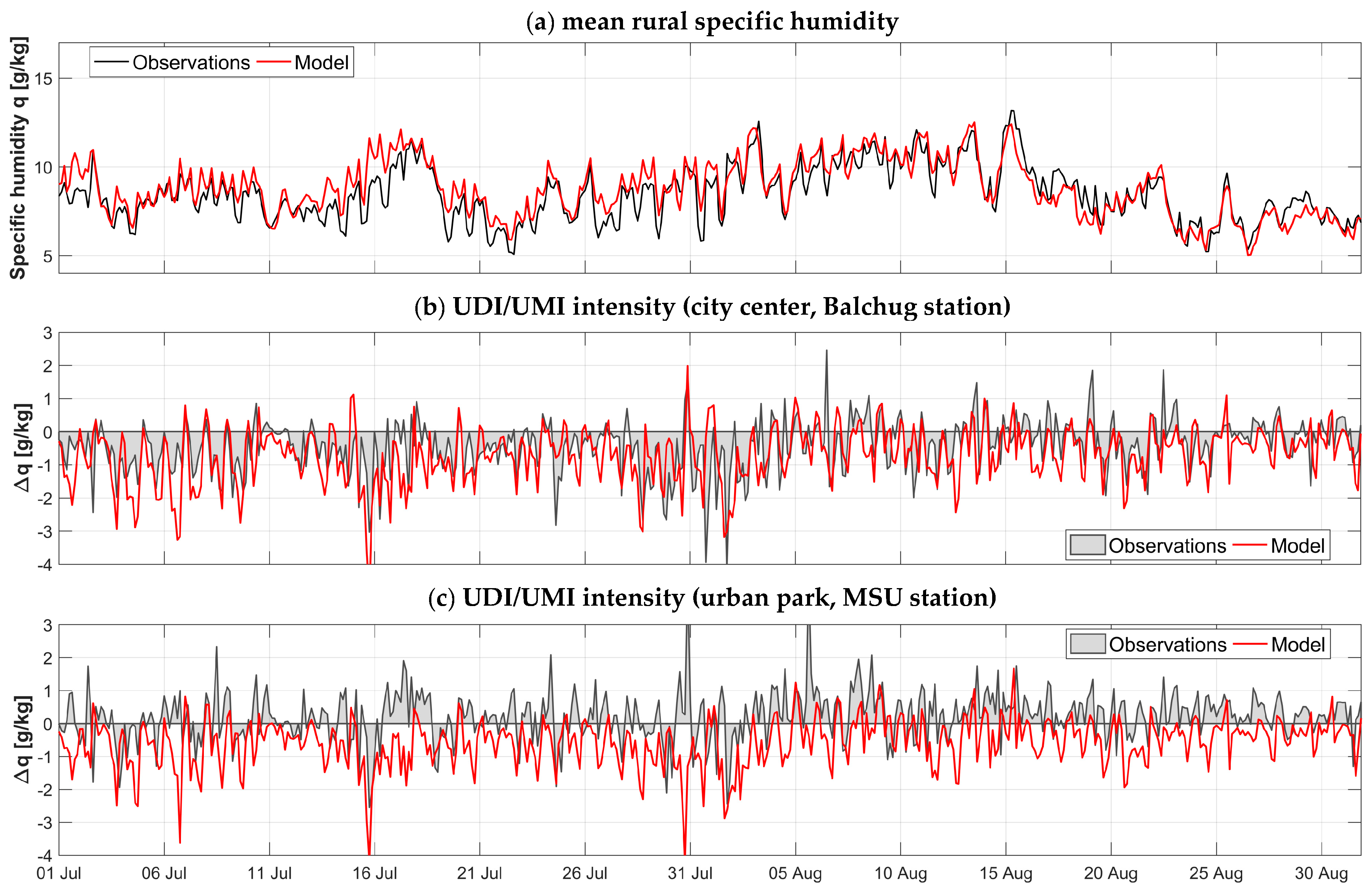
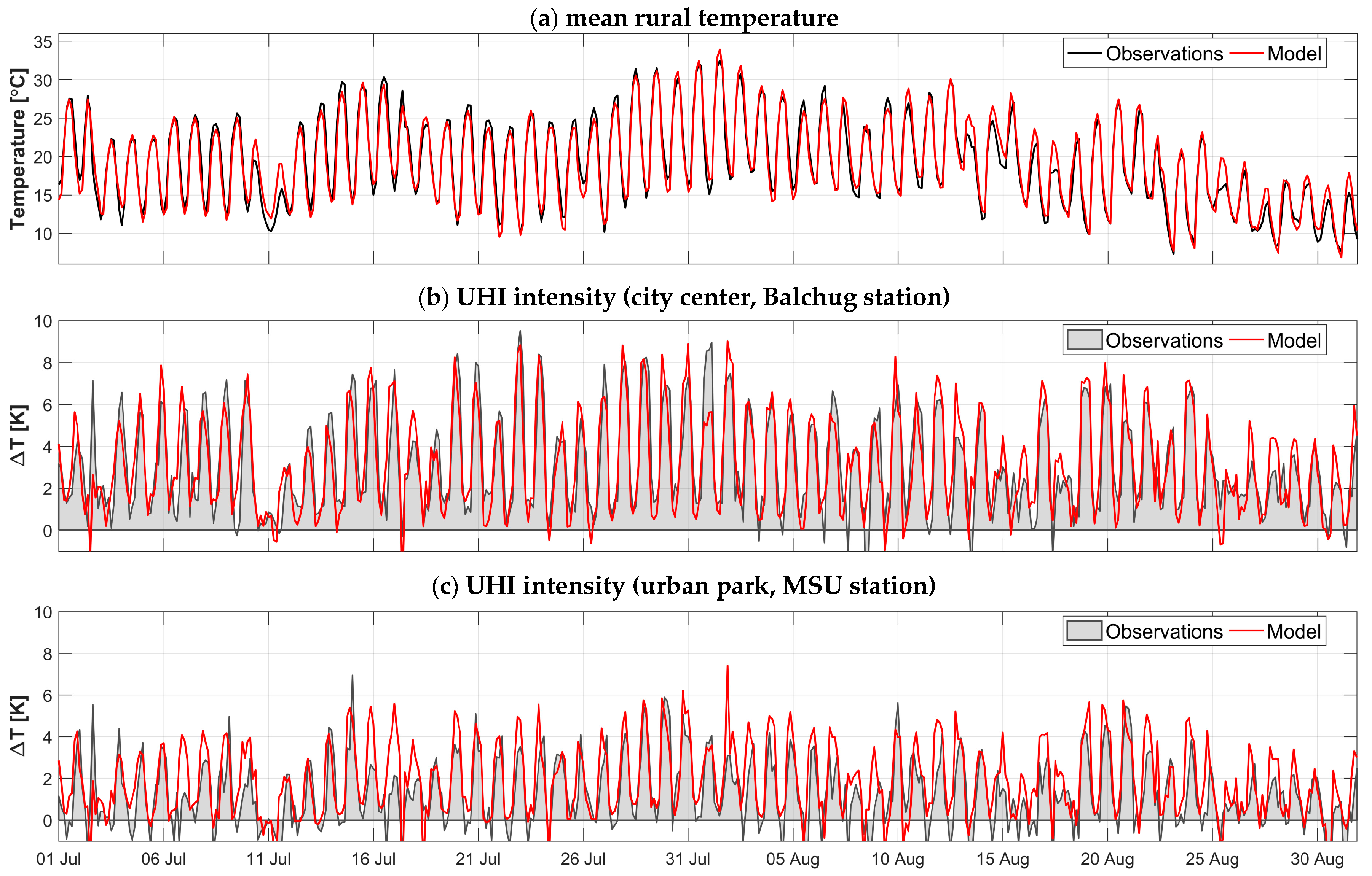
3.1. Model Verification Based on Canopy-Layer Observations

Verification of the model ability to simulate the key features of investigated phenomena is an essential part of modeling studies. Since the canopy-layer UHI and UDI/UMI intensities are considered as important for most of the studied features of urban climate, model-to-observations comparison was performed for this variables in addition to rural values of near-surface (2 m) air temperature and specific humidity. The observed canopy-layer UHI and UDI/UMI intensities were defined as deviations from the mean temperature and humidity over nine rural stations (for humidity, positive deviation indicates UMI while negative deviation indicates UDI). Such values were calculated separately for the city center (Balchug station) and the urban park (MSU). Modeled values for such comparison were calculated in the same way based on the “URB” simulations for the corresponding model cells, selected among the nine nearest cells around each of the weather stations. For Balchug station, we used the temperature and humidity values that were modeled for the urban tile in the nearest densely built urban cell. For MSU station, we used such values for the natural tile of the nearest semi-urban cell (UF ≈ 50%), and for the rural stations the values for the nearest non-urban cells were used.

Figure 2 shows the model-to-observation comparison for mean rural temperature and UHI intensity for two urban sites, while Figure 3 shows the same for the rural specific humidity and UDI/UMI intensity. Such comparison indicates a good agreement between modeled and observed values in terms of temporal variation (on diurnal and day-to-day timescales), average values and typical extremes, including high UHI intensity values reaching up to 10 K. The only significant bias is a systematic underestimation of the urban–rural moisture difference (an overestimation of the daytime UDI intensity and underestimating of the nocturnal UMI intensity), which is discussed in Section 3.4.

We would like to highlight that such a good quality of replication of observations by the model was achieved using the optimized model configuration described in [30]. In addition, that study reports the good agreement between the modeling results and observations for Moscow for other summer seasons in terms of the temperature, UHI intensity and summer precipitation amounts. Additionally, it proves the adequacy of the simulations of the UHI spatial structure based on comparison between modeling results and data of the newest detailed observational networks.

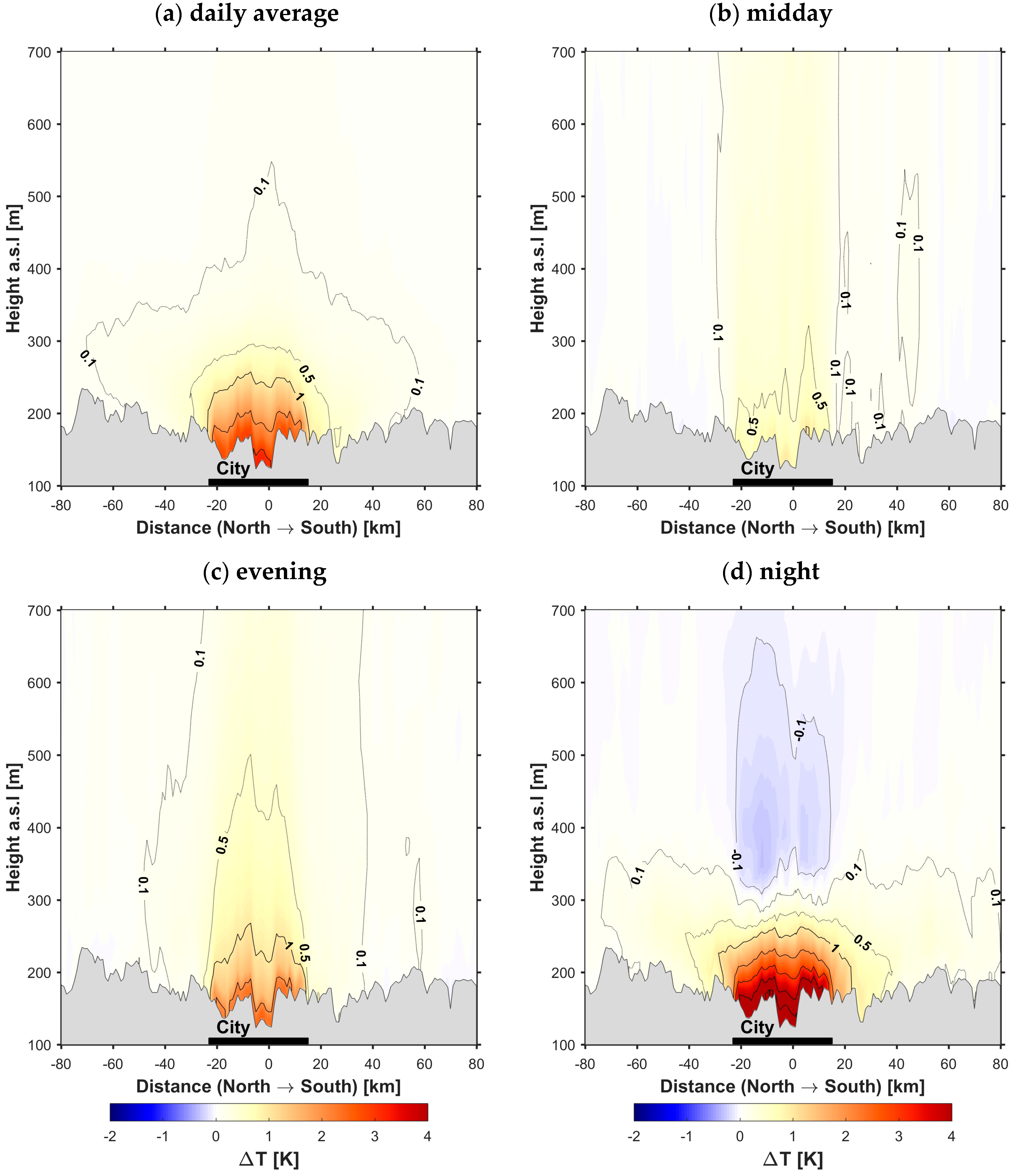
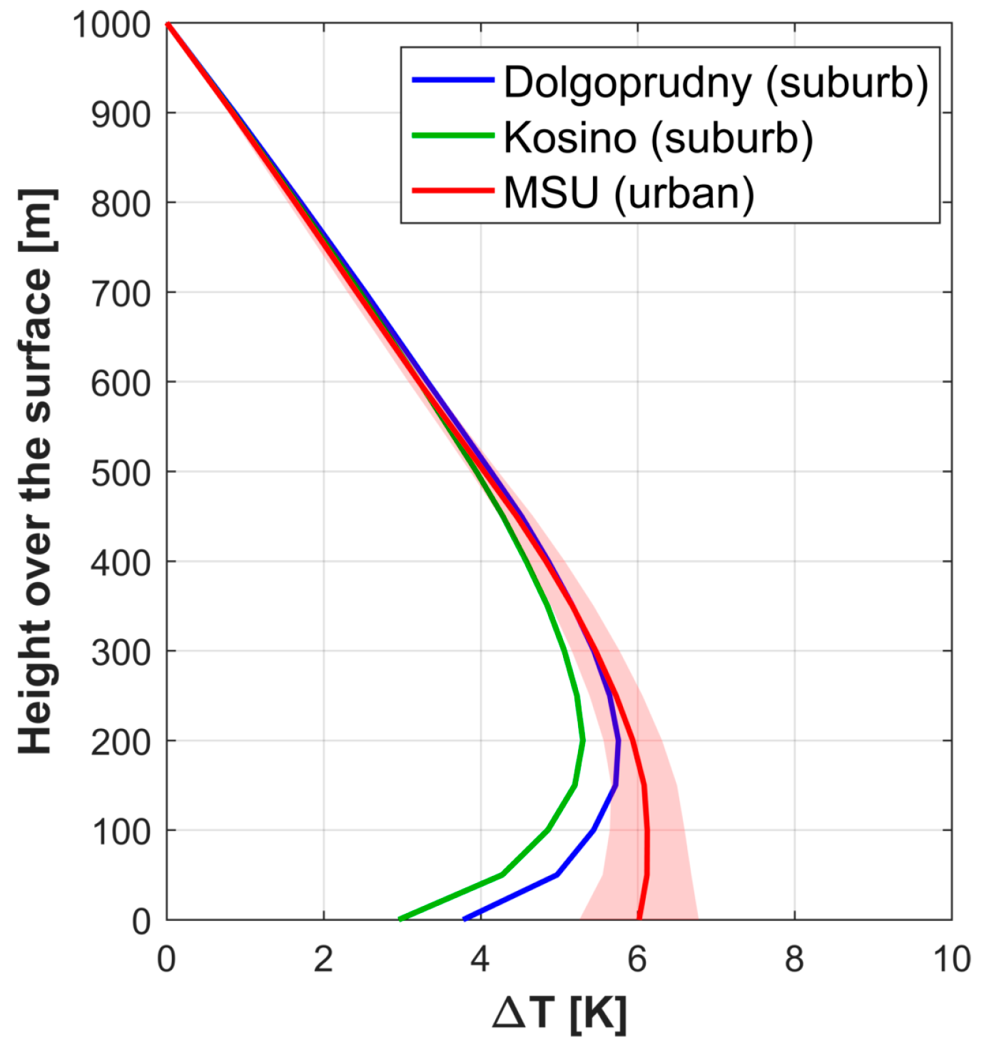
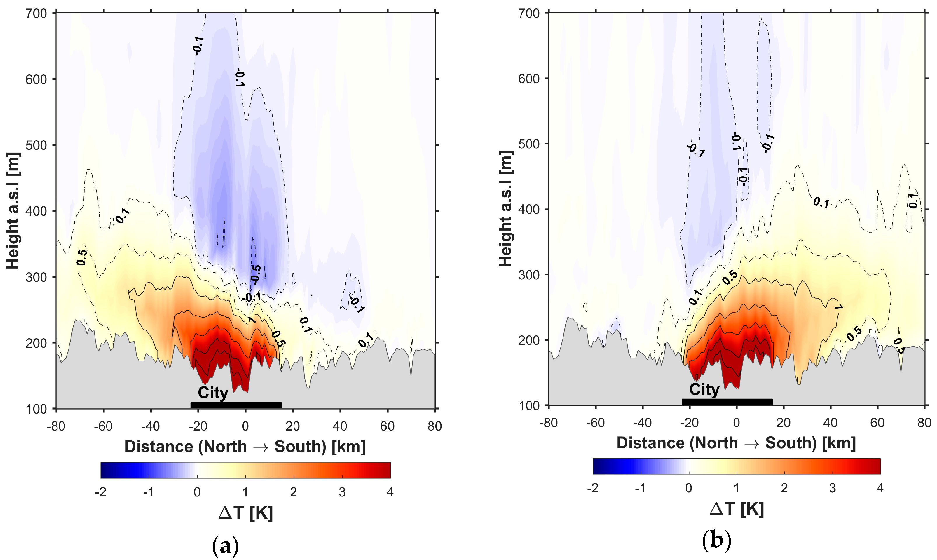
3.2. Vertical Structure of the UHI

The vertical cross-sections trough the city center in field of temperature response to switching on the UCM (Figure 4), calculated as described in the Section 2.5, shows that daily-average UHI vertical extent reaches 250–400 m. Daytime (12 UTC/15 MSK) UHI extends up to 1–1.5 km, but its intensity even near the surface does not exceed 0.5 K. In the evening (16 UTC/19 MSK), UHI has similar vertical extent and strengthens within lower 400 m.

Intensive nocturnal (0 UTC/3 MSK) UHI exists only within thin (100–150 m) layer and is overlaid by a layer with negative temperature response that indicates a so-called cross-over effect [21] or cold lens [34]. Its appearance could be explained by more intensive vertical mixing and upward motions over the city in conditions of stable stratification [74]. The other explanation is the divergence of longwave radiation flux, typical for more moist and polluted urban air over the city [34,75]. However, these factors do not play a significant role in the model because urban features of atmospheric composition are not considered, while urban humidity is underestimated by the model (see Section 3.1 and Section 3.4).

The existing measurement campaigns for Moscow region makes a qualitative comparison possible between the modeling and the observational results. According to the recent study based on the data of contact measurements (analyzed on annual basis only) [22], daily average value of UHI vertical extent is ≈300 m and nocturnal crossover effect is identified higher than 100 m over the surface. Recent studies, based on the satellite remote sensing data [1,35,36], report that UHI vertical extent at midday and evening hours during the summer is 1.5–2 km, which agrees with modeling results for this time of the day.

Another estimation of UHI vertical extent could be obtained from the measurements of microwave temperature profilers MTP-5 [76,77], operating in Moscow region [34,78]. The most relevant in the scope of this study are recent results [79], based on synchronous observations at urban park located close to city center (MSU site) and two suburb sites (Dolgoprudny and Kosino) during the warm season (April–July) of 2015. The average day-time temperature profiles over these sites are very similar in terms of vertical gradients. At the same time, the mean profiles over selection of nocturnal hours with pronounced canopy-layer UHI clearly show its vertical extent up to 200 m (Figure 5), which agrees with modeling results. Nocturnal crossover effect is not identified by these observations, which could be explained by its low magnitude or its spread over the nearest suburbs.

The qualitative agreement between modeling results, listed observations for Moscow megacity and also simulations for Paris within different modeling framework [32] gives us confidence that the COSMO-CLM model coupled to TERRA_URB UCM adequately simulates the UHI in the ABL and the precursor urban–atmospheric interactions. Thus, the additional features of the urban troposphere are investigated below.

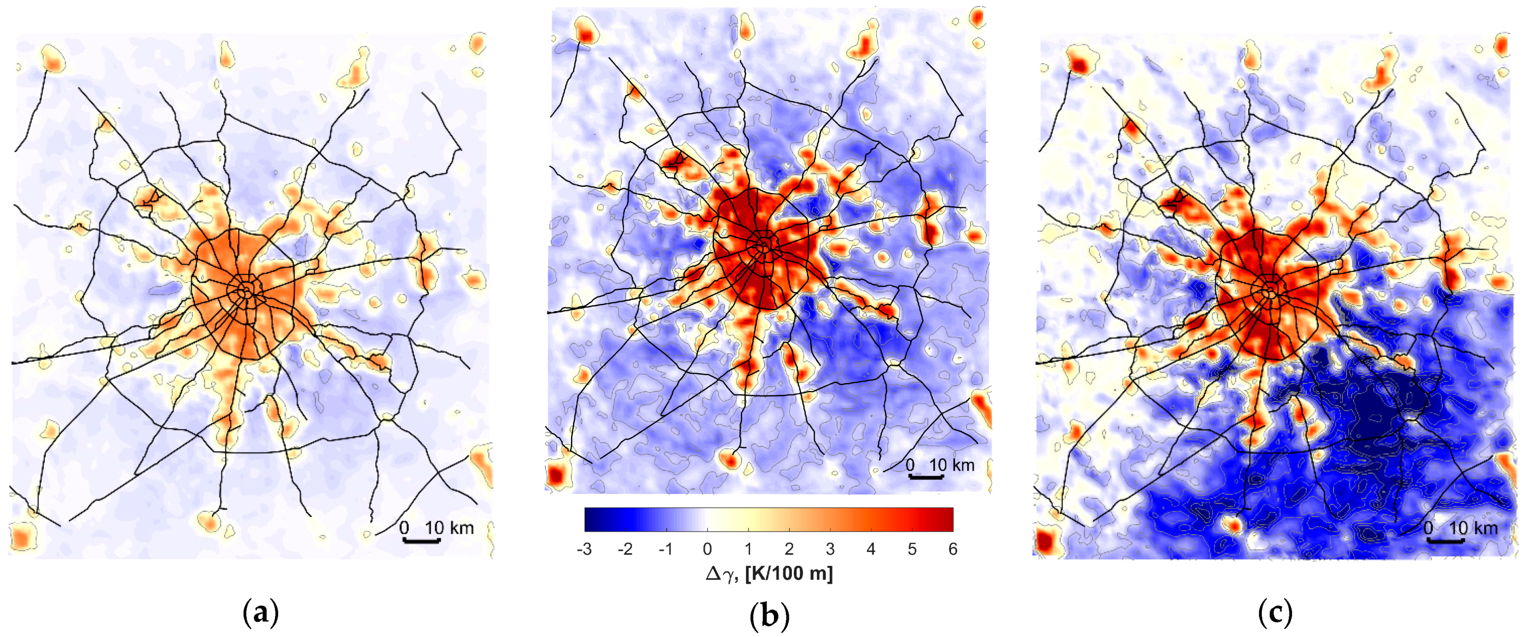
3.3. Urban Heat Plumes

The modeling results clearly demonstrate urban heat plumes (UHP) [80] downwind of Moscow. Their existence follows from general features of ABL dynamic over inhomogeneous landscapes: warm urban air is carried by the wind, interacts with the colder and more stable suburban internal boundary layer and is pushed upward, which forms the elevated urban plume. While the influence of wind direction on the shape of the near-surface UHI is reported in the number of studies (e.g., [79,81,82]), three-dimensional structure of UHPs is practically unstudied. Probably, the only experimental proofs of their existence are based on the data of helicopter and airplane sounding over American cities for certain case-studies [23,80].

The modeling results allow us to obtain the more detailed vertical structure of the UHI and those UHP under different wind directions. The classification of the cases by wind direction is performed based on the mean wind direction within the lowest 150 m above the ground over the whole D3 domain (four lowest model levels). The results are grouped for prevailing northern (315–45°), eastern (45–135°), southern (135–225°) and western (225–315°) wind direction and for each hour. Vertical cross-sections of the temperature response, averages for such selections, shows that the UHI is shifted by an incoming stream to the lee side of the city for the entire day. This effect is most evidently pronounced at night and in the early morning.

At the same time, the formation of elevated UHPs downwind to the city is observed. They are most pronounced between 0 and 4 UTC (3–7 MSK), stretching for tens of km (Figure 6). The spatial structure of the UHI wind shear and UHPs also features the Ekman wind rotation with altitude (Figure S2). For example, the UHI at the lowest model level is shifted to northwest for the selection of nocturnal cases with prevailing northern wind and to southeast for the selection of cases with southern wind. With increasing altitude, the shear direction turns right following the wind rotation.

In addition, the non-trivial effect of the UHPs on thermal stratification over rural areas was revealed. It is well-known that thermal stratification over the cities is in general more unstable than over rural areas due to higher buoyancy of warmer urban air. The modeling results reproduce this pattern: the response of the lapse rate ($\gamma =-dT/dz$), calculated between two lowest model levels (10 and 35 m) is positive over urbanized model cells (Figure 7a,b). However, over the nearby rural areas negative responses are observed. In other words, influence of the big city makes the atmosphere more stable over surrounding rural areas. Such model behavior is related to the UHPs. This is clearly illustrated by mean values of lapse rate response over selection of cases with prevailing northern wind (Figure 7c).

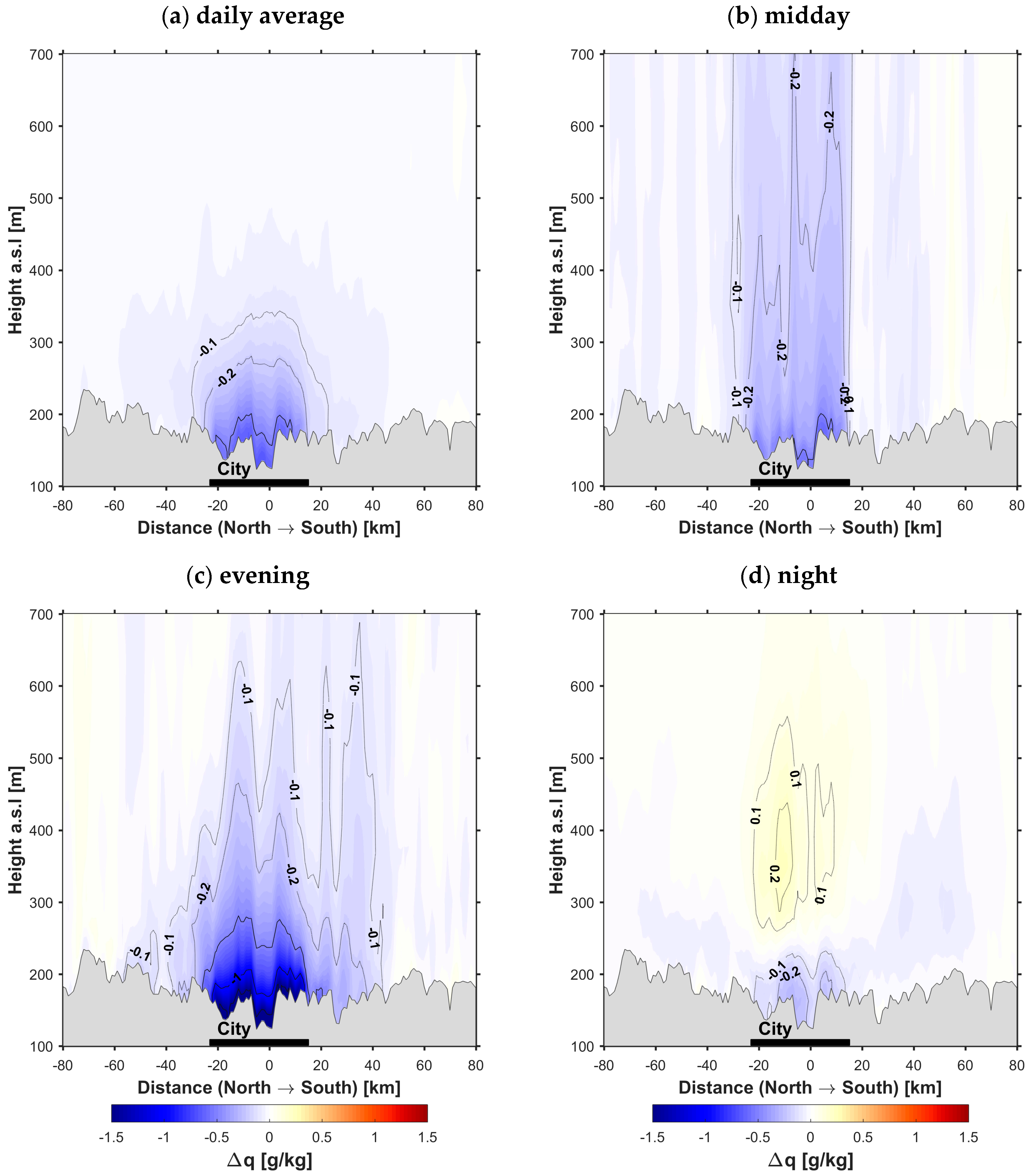
3.4. Vertical Structure of the UDI/UMI

The spatiotemporal variation of the UDI is partially similar to the UHI following general features of ABL diurnal dynamics. However, it is affected by negative phase shift: the maximum of canopy-layer UDI intensity is reached at the evening instead night, which is consistent with classic studies [11,12,15] and observations for Moscow [36]. The negative daily-mean specific humidity response also has a domed shape and extends up to 200–250 m over the city center (Figure 8).

During the day-time, UDI grows up to 1–1.5 km, becomes the most intensive near the surface in the evening and weakens at night. This agrees with existing studies reporting near-zero or even positive (UMI effect) nocturnal urban–rural moisture differences, caused by later and less often reaching the dew point by warmer urban air [15]. Nocturnal UMI effect is often detected in Moscow [36], however near-surface urban moisture seems to be underestimated by the model (Figure 3). This could originate from the fact that model does not take into account the vegetation in street canyons and anthropogenic moisture release. Consequently, near-surface UMI could not be detected in the mean seasonal values. However, it is detected above the surface, at the same height as elevated negative temperature response stemming from the cross-over effect.

The only observational study devoted to vertical structure of UDI/UMI over Moscow [36] is based on satellite remote sensing data and reports similar patterns of spatiotemporal variations of summer-time urban–rural moisture differences, but with more pronounced humidity cross-over effect at the evening. Significantly weaker midday humidity cross-over effect, also detected according to remote sensing data, is not reproduced by the model. This is consistent with the fact that the overall underestimation of the modeled urban humidity mentioned above. It should be noted that much more pronounced day-time humidity crossover effect is detected according to WRF simulations for London [33], however even the qualitative comparison in this case is incorrect because of different climate features of Moscow and London (Dfb and Cfb types according to Köppen classification, respectively) and because of the absence of any observational evidence for London.

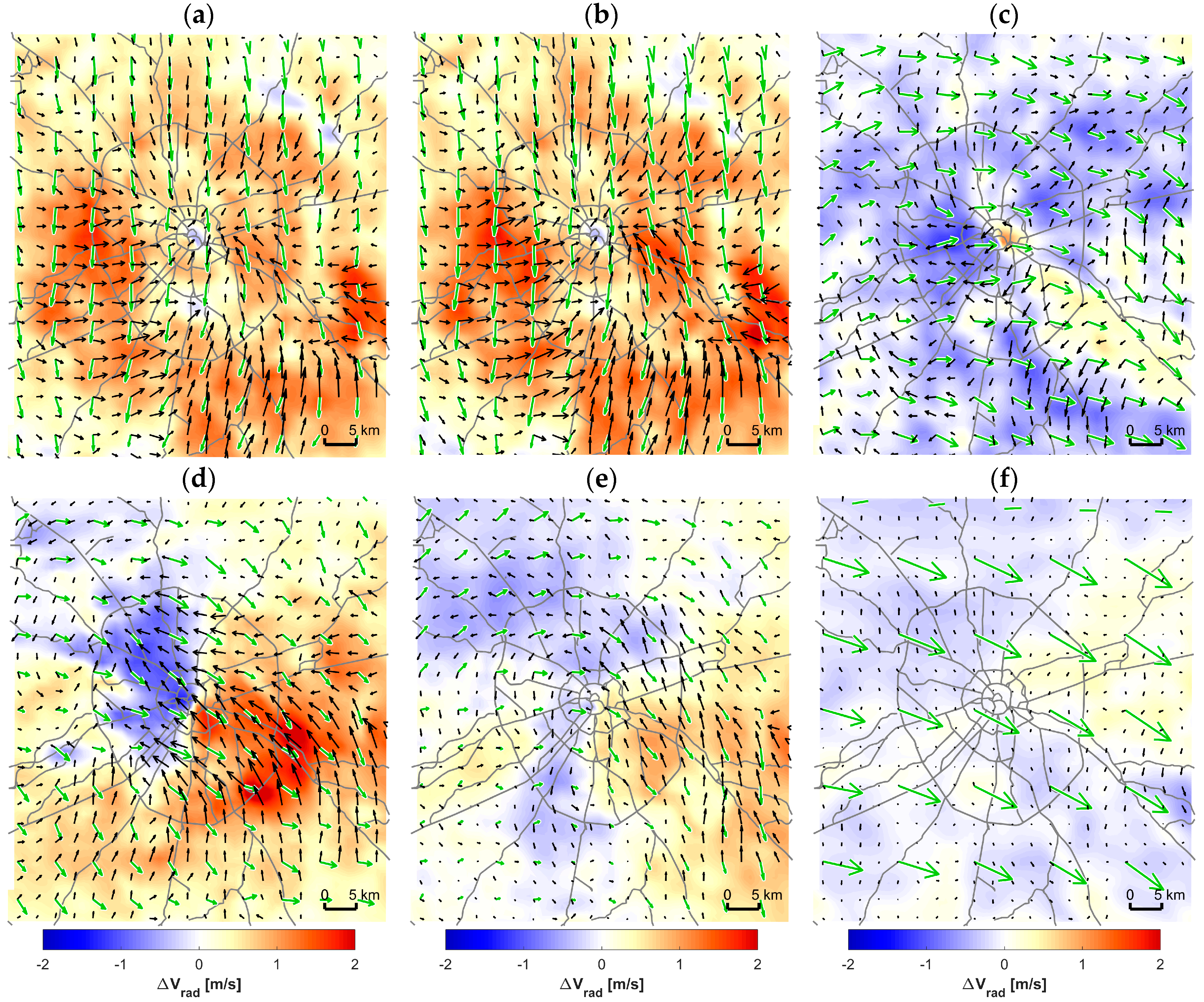
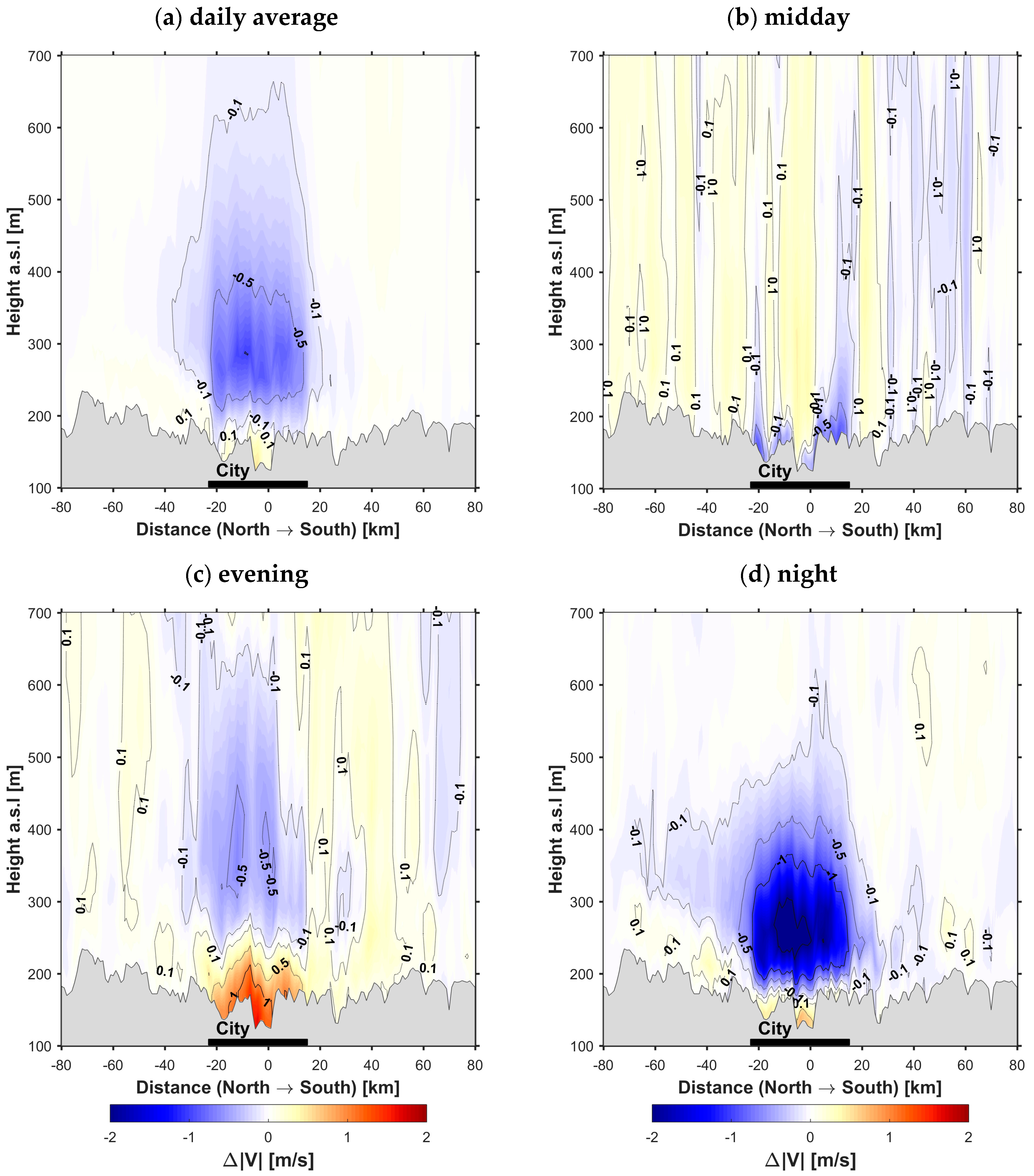
3.5. Urban Effects on Wind Speed and Mesoscale Circulation

Existing studies have noted decrease of the mean near-surface wind speed for urban areas due to higher roughness [11,12,83], which, in general, should extend upward to the ABL. Our modeling results confirm this by negative wind speed response over the city, which is the most pronounced at 150–200 m above the surface (Figure 9). At night, this is more pronounced (within 100–300 m above the ground), but no systematic response could be found at midday. During the evening, the negative response is also observed at 100 m above the ground onwards. Surprisingly, it turns positive between 0 and 100 m during the evening (up to 1.5 m/s on average) and also slightly during the night.

Such effect could be caused by another factor altering the wind regime over urban areas, related to urban-induced mesoscale circulations known as the urban breeze. Such circulations appear following the urban effects on stratification and upward motions. However, their existence is proven only by limited number of observational studies (e.g., [12,23,25]), idealistic laboratory and numerical experiments [84,85] or mesoscale simulations for certain case studies [24]. Its influence on wind climatology is practically unstudied, and it has only been reported that the wind speed within urban canopy could be higher that over rural areas at calm evenings and nights [11,12,86].

To investigate whether the modeled positive wind speed response is related with urban breeze, radial (directed to the city center) wind speed component:

$$V_{rad}=-V·cos(D-D_c)$$

(2)

where $V$ is absolute wind speed for each model cell, $D$ is the wind direction, and $D_c$ is the direction to city center.

In addition to the main selection of cases (days with pronounced UHI during summer 2014), cases with calm weather (mean wind speed within the lowest 150 m over whole D3 domain <3 m/s) were sampled out of the main selection separately for each hour of the day. This results 7–30 cases for each hour.

Temporal and vertical variations of the modeled responses of the wind speed and its radial component, averaged over the Moscow region (within the area extending by 50 and 40 km in latitude and longitude directions correspondingly), show that a positive wind speed response is accompanied by a positive response of its radial component, which is most pronounced in the evening, especially for calm weather conditions (Figure S3). Negative response of radial wind speed component, corresponding to “anti-breeze” part of urban-induced circulation, is detected in the evening higher than 1 km.

Such patterns are confirmed by spatial structure of vector field of the wind response to switching on the UCM. The amplification of wind convergence to the city center at lowest model levels is identified over whole urban area for evening cases with low wind speed (Figure 10a,b). Such pattern is in good agreement with results of idealized studies [84,85]. Wind divergence is amplified at the height over 1.5 km (Figure 10c), but spatial structure of the response is more complicated, probably because of interactions with much stronger background flow.

For nocturnal hours with maximum surface-layer UHI intensity, existence of pronounced urban breeze could be also suggested. However, the spatial patterns of the nocturnal wind response are more complicated (Figure 10d,e). They are much stronger affected by the inhibition of incoming air flow, which is characterized by northwestern direction. The magnitude of the wind response vector at southeastern part of the city exceeded the speed of undisturbed flow according to “noURB” simulations. Another interesting feature of nocturnal wind response is the amplification of cyclonic vorticity over the city at the height about 120 m (Figure 10d). Nocturnal “anti-breeze” effect is not pronounced (Figure 10f). Understanding the drivers of such response requires a separate, more detailed analysis.

It should be noted that similar spatial patterns of vector field of the wind response (with quite lower magnitude) are identified in the fields of mean values over much bigger selection of cases without respect to the background wind speed (Figure S4). As such, urban breeze effect is found to be a systematic urban mesoclimatic feature of Moscow.

Quantitative or even qualitative comparison between modeling results and observations in terms of urban breeze features is impossible for Moscow because of the absence of any previous urban breeze studies. Modeling study for Paris megacity [24] reports similar patterns of the late-afternoon urban breeze and its absence during the night with intensive UHI. Urban-induced wind speed amplification reported for Paris (5–7 m/s) is significantly stronger than revealed in this study. However, results for Paris characterize the specially selected case with favorable conditions instead of averaged over several formally selected cases for Moscow, and extreme values of the wind speed response for Moscow are comparable with those reported for Paris (not shown).

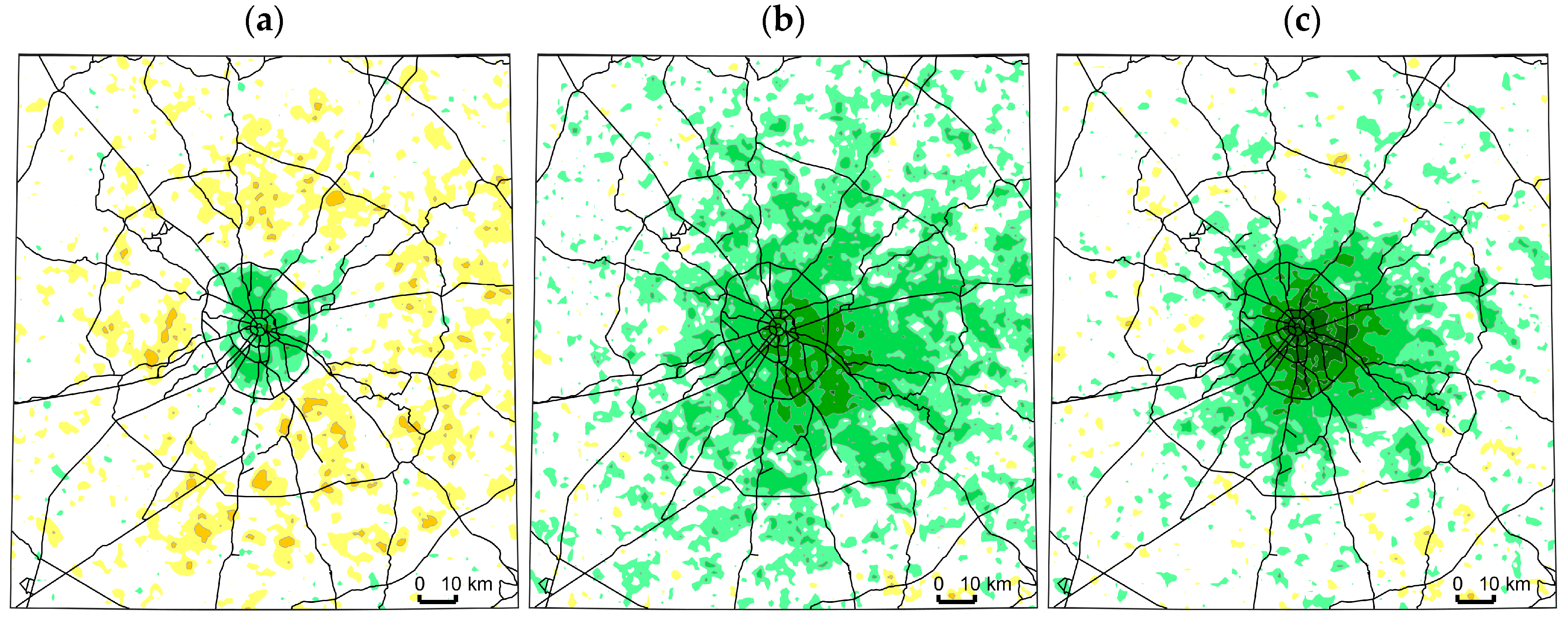
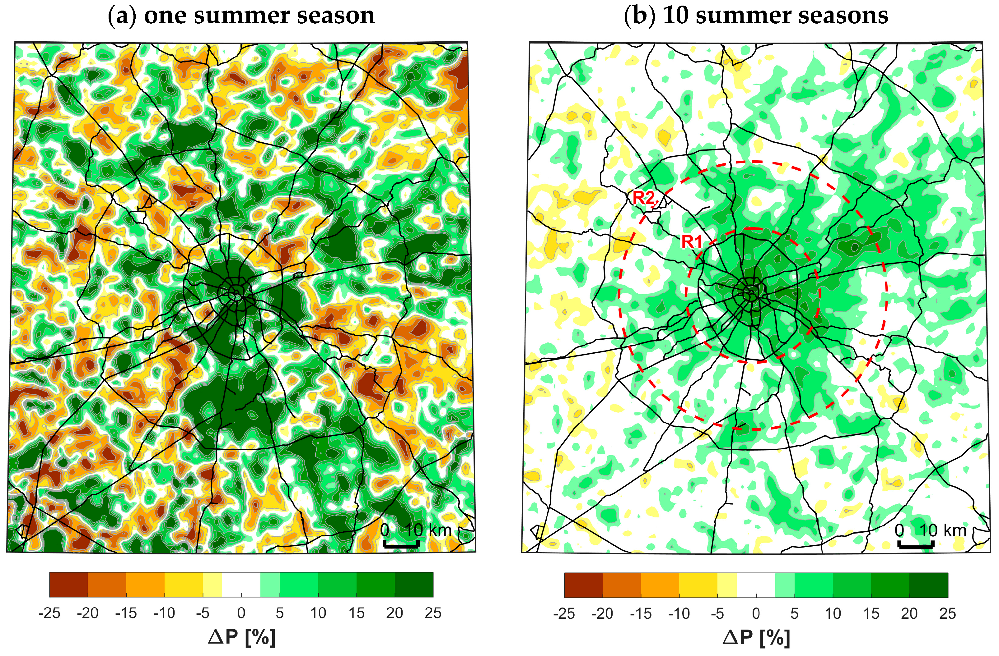
3.6. Urban Effects on Precipitation and Cloudiness

The modeled summer precipitation response to switching on the UCM, accumulated over a certain summer season, is characterized by a chaotic spatial structure (Figure 11a), which could be explained by the stochastic nature of summer convective showers. However, the noise pattern decreases when increasing the averaging period. Averaging over ten summer seasons allows us to clearly identify a positive precipitation response over the city and its surrounding (Figure 11b).

Switching on the UCM increases the mean summer precipitation amount within R1 area (20 km from the city center, see Figure 11b) by 10% in relation to the results of “noURB” simulations, with local maxima up to 25%. Within the distance from 20 to 40 km from the center (R2 area), the mean response value is only ≈4%. However, local maxima up to 25% are also found to the east and northeast of the city, which is its leeward side relative to prevailing western winds. Values of such responses (means over R1 and R2 areas) have a significant inter-annual variability as described in more detail in [48], however they are positive for each among the ten considered summer seasons.

Presented modeling results agrees with a number of studies reporting the urban-induced amplification of convective precipitation due to additional triggering of the moist convection (e.g., [26,27,28,29]). Midday and evening maximum in the daily course of the precipitation response (Figure S5) additionally supports its connection with urban-induced intensification of convective processes. Additionally, such hypothesis is supported by the presence of the positive response of day-time and evening cloudiness, also shifted to the eastern leeward side of the city (Figure 12). This pattern is detected for total, low-level, mid-level and upper-level cloudiness (accordingly, CLCT and CLCL model variables).

Surprisingly, a negative response of the nocturnal low-level cloudiness is simulated by the model over the city (not shown). It is probably caused by the fact that fog and haze (diagnosed as low-level clouds), frequently present over the rural areas during summer nights and occur less frequent due to the UHI that inhibits condensation. However, these processes are not fully understood and need to be analyzed in more detail in future research. This is one reason why daily-mean and nocturnal cloudiness is not analyzed in details.

Existing studies for Moscow also report the urban-caused enhancement of the summer precipitation, however its quantities estimates vary significantly. According to the data of the dense network of the weather stations, which existed in Moscow city during the 1950s–1960s, the summer precipitation amounts in the city exceed those for surrounding rural areas by 20% [87], while the more recent studies bases on smaller number of weather stations report increase of only 8% [88] or even close to zero [89]. However, such variation of the estimates looks reasonable due to very high spatial and temporal variations of the urban–rural precipitation differences, as reported in [88] and confirmed by presented modeling results.

Modeled responses of day-time cloudiness are in good quantitative and qualitative agreement with remote sensing data for Moscow [90] (increase up to 0.4 tenth for daytime total cloudiness over the city in the model and ≈0.6 tenth according to observations).

4. Discussion

Urban-caused meteorological phenomena, considered within the current study (UHI, UDI and UMI, urban heat plumes and urban breeze, urban enhancement of precipitation and cloudiness) were previously known according to theoretical assumptions, several observational and modeling studies, and idealistic numerical and laboratory experiments. This is the first time that they were analyzed together within similar modeling and data-processing framework based on continuous high-resolution mesoscale simulations, conducted for multiple summer seasons.

In contrast to a wide part of previous studies, presented results shows that the megacity-induced meteorological effects in the lower troposphere persist, not only for certain case studies with favorable conditions, but also for the seasonal means or means over specific selection of the cases, performed in formal ways (e.g., according to wind direction or speed).

Although the detailed analysis of three-dimensional variables (temperature, humidity and wind components) was made only for one summer season (2014) due to technical limitations, preliminary results for other summer seasons shows very similar patterns, which supports the significance of presented estimates and allows to consider them as “quasi-climatologic”. However, the urban effect on precipitation and cloudiness cannot be adequately diagnosed from one summer due to the stochastic nature of convective systems. Only the averaging for 10 seasons allows us to detect the urban effects on the precipitation amounts and cloudiness. This demonstrates that the consideration of (quasi-)climatological timescales is required for providing conclusive results about such effects.

In further studies, the developed framework of modeling and data analysis will allow us to make a more robust statistical analysis of the revealed mesoclimatic effects based on the data for longer period, including other seasons. This will allow us to go from “quasi-climatic” estimates of urban-induced meteorological effects to their actual climatology.

Some of the presented results (the UHI and its vertical extent, urban breeze circulation, and urban enhancement of precipitation and cloudiness) are supported by earlier observational and modeling studies for Moscow and other big cities, hence confirming their relevance. This opens a wide perspective for more detailed quantitative comparison between modeling results and observational data of existing and new measurement campaigns for Moscow megacity, which seems to be a useful testbed for the verification of urban climate models.

Key scientific value of presented results, in our opinion, is related to the clarification of the various feedbacks and interrelations in the ABL and lower troposphere, interacting with urban climate features. In contrast to a number of studies, focusing on micrometeorological regime canopy layer and considering its features as a function only from land-use and building parameters (e.g., [91,92,93]), we show that the megacity climate features are expressed as mesoscale phenomena and affected by tropospheric feedbacks, including advection, diffusion, urban-induced mesoscale circulations and perturbations of atmospheric convection. These findings are in good agreement with previous modeling studies reporting the presence of non-local mesoscale feedbacks to urban expansion [7,30]. The revealed Coriolis-forced veering of the UHI downwind shift by the Ekman layer wind rotation and amplification of cyclonic vorticity seems to be a new finding, not shown in existing studies, which requires more detailed investigation.

Special attention should be paid to our urban modeling results that revealed a systematic urban-induced enhancement of precipitation and daytime cloudiness over the 10 summers. In the number of previous studies about the urban features of atmospheric composition, the higher aerosol concentrations were considered as important factors of urban-induced precipitation increase [28,87,94]. However, the current modeling experiments were performed without considering aerosol effects. This shows that urban precipitation enhancement is at least partially caused by pure physical (dynamical) mechanisms induced by surface temperature, humidity and roughness features. Such effect found in our results is consistent with the well-known “negative spatial soil moisture–precipitation coupling” (see, e.g., [95,96,97,98]) indicating that precipitation occurs preferentially over those patches—in our case, Moscow megacity—that are relatively drier than the surroundings. The mechanisms of urban-induced precipitation evidently require more detailed investigation in further studies, however their linkage with urban breeze circulation and urban effect on the lapse rate could be suggested.

From a practical point of view, presented results show the importance of taking the revealed urban-induced meteorological effects and urban climate features into account in various weather, air quality and climate services, not only for the cities, but also for their rural outskirts. Particularly, the revealed enhancement of stable stratification over downwind urban areas could affect the features of pollutants dispersion. Urban breeze circulation is another factor probably enhancing the ventilation of the city, while at the same time promoting the pollutants transfer from industrial areas, located in suburbs, to the city center. Thus, urban-induced processes should be essentially considered in air quality forecasts for urban areas, e.g., in COSMO-ART model [99], which is now used for this purpose for Moscow region [100,101]. It is also important to take them into consideration in high-resolution weather forecast for urban areas, biometeorological applications and in downscaling of climate change scenarios as shown in [7,102].

The complex analysis of the presented urban-induced mesoclimatic effects, performed for Moscow megacity, could be a demonstrative illustration for future mega-city climate modeling and data processing frameworks, which shows:

(1)

the variety of the urban–atmosphere feedbacks affecting the urban climate features;

(2)

the importance of further research on in-depth understanding of these feedbacks, which would foster better forecasts and more effective urban climate adaption; and

(3)

the significance of taking them into account in various weather and climate services and applications, including weather and air-quality forecasts, modeling studies in field of biometeorology and the climate change assessments for urban areas.

5. Conclusions

Using the COSMO-CLM mesoscale model coupled to the urban canopy scheme (UCM) TERRA_URB at the horizontal resolution of 1 km, the urban-induced mesoclimatic effects in the lower atmosphere over Moscow megacity were analyzed for the summer season on continuous time-scales (July–August 2014 for three-dimensional fields of the temperature, humidity and wind, and 10 summer seasons for precipitation and cloudiness). Such effects were investigated as differences between the modeling results for present-day urban surface characteristics calculated according to OpenStreetMaps data and the results of the additional model runs with the UCM switched off.

The model-to-observation comparison shows that temperature and humidity and their respective urban–rural differences are simulated very well, except for a negative bias for the specific humidity in the city. Moreover, the vertical extent of the UHI also agrees qualitatively well with existing studies including the recent results based on the observations of three similar microwave temperature profilers in the city and its suburbs.

Our simulations revealed that the urban effects on the temperature, humidity and wind extends to the lower troposphere at least for 1–2 km and are affected by various atmospheric feedbacks, which defines the complicated spatiotemporal dynamics of such effects. Particularly, the day-time UHI is characterized by a weak intensity (≈0.5 K) and pronounced vertical extent (≈1.5 km). The nocturnal UHI is more intense (>3 K) and confined close to the ground (vertical extent ≈150 m), while cooling above (at the height ≈200–700 m above the ground) is established by the cross-over effect. The urban effects on moisture are characterized by similar vertical extent and negative phase shift in comparison to the UHI. The pronounced daytime and evening UDI extends up to 1–1.5 km, while the nocturnal elevated UMI is formed at same height as the evaluated cooling effect. The spatial structure of the UHI is shifted downwind of the city, and such shift is modulated by a double Coriolis effect resulting from the Eckman-layer forcing and additionally from cyclonic-vorticity forcing. Moreover, pronounced elevated heat plumes are formed downwind of the city during the night. They extend for tens of kilometers and significantly enhanced the stable stratification over rural surroundings.

The urban effects on wind also extend vertically up to 1–2 km above the ground and are characterized by: (1) a lower wind speed due to higher surface roughness; and (2) an amplification of the near-surface wind convergence around the thermal low known as the urban-breeze effect. The latter is most pronounced during the evening. On calm days, such effect results in a significant increase of the wind speed near the surface, which is also identified in terms of seasonal mean values. The urban-induced circulations are not so pronounced during the night and have more complicated spatial patterns, which are not fully understood. Particularly, they result in the amplification of the cyclonic vorticity around the city detected at the height of ≈ 100–150 m over the surface.

By addressing the quasi-climatological scales considering 10 summer seasons, our analysis has revealed a significant influence of the city on the dynamic processes in the lower troposphere by the enhanced precipitation and cloudiness over the city and its leeward side. Herein, the mean summer precipitation amount is increased by 10% over the city with local extremes up to 25%. Similar patterns are identified for the day-time total and low cloudiness.

References

- Kislov, A.V.; Varentsov, M.I.; Gorlach, I.A.; Alekseeva, L.I. “Heat island” of the Moscow agglomeration and the urban-induced amplification of global warming. Moscow Univ. Vestnik Ser. 5 Geogr. 2017, 4, 12–19. (In Russian) [Google Scholar]
- Ren, G.Y.; Chu, Z.Y.; Chen, Z.H.; Ren, Y.Y. Implications of temporal change in urban heat island intensity observed at Beijing and Wuhan stations. Geophys. Res. Lett. 2007, 34. [Google Scholar] [CrossRef]
- Kalnay, E.; Ming, C. Impact of urbanization and land-use change on climate. Nature 2003, 423, 528–531. [Google Scholar] [CrossRef] [PubMed]
- Schatz, J.; Kucharik, C.J. Urban climate effects on extreme temperatures in Madison, Wisconsin, USA. Environ. Res. Lett. 2015, 10, 94024. [Google Scholar] [CrossRef]
- De Ridder, K.; Maiheu, B.; Lauwaet, D.; Daglis, I.; Keramitsoglou, I.; Kourtidis, K.; Manunta, P.; Paganini, M. Urban Heat Island Intensification during Hot Spells—The Case of Paris during the Summer of 2003. Urban Sci. 2016, 1, 3. [Google Scholar] [CrossRef]
- Konstantinov, P.I.; Varentsov, M.I.; Malinina, E.P. Modeling of thermal comfort conditions inside the urban boundary layer during Moscow’s 2010 summer heat wave (case-study). Urban Clim. 2014, 10, 563–572. [Google Scholar] [CrossRef]
- Wouters, H.; De Ridder, K.; Poelmans, L.; Willems, P.; Brouwers, J.; Hosseinzadehtalaei, P.; Tabari, H.; Vanden Broucke, S.; van Lipzig, N.P.M.; Demuzere, M. Heat stress increase under climate change twice as large in cities as in rural areas: A study for a densely populated midlatitude maritime region. Geophys. Res. Lett. 2017, 44, 8997–9007. [Google Scholar] [CrossRef]
- Tan, J.; Zheng, Y.; Tang, X.; Guo, C.; Li, L.; Song, G.; Zhen, X.; Yuan, D.; Kalkstein, A.J.; Li, F.; et al. The urban heat island and its impact on heat waves and human health in Shanghai. Int. J. Biometeorol. 2010, 54, 75–84. [Google Scholar] [CrossRef] [PubMed]
- Buechley, R.W.; Van Bruggen, J.; Truppi, L.E. Heat island = death island? Environ. Res. 1972, 5, 85–92. [Google Scholar] [CrossRef]
- Dousset, B.; Gourmelon, F.; Laaidi, K.; Zeghnoun, A.; Giraudet, E.; Bretin, P.; Mauri, E.; Vandentorren, S. Satellite monitoring of summer heat waves in the Paris metropolitan area. Int. J. Climatol. 2011, 31, 313–323. [Google Scholar] [CrossRef]
- Oke, T.R. Boundary Layer Climates, 2nd ed.; Routledge: Abingdon-on-Thames, UK, 1987; ISBN 0203407210. [Google Scholar]
- Landsberg, H.E. The Urban Climate; Academic Press: Cambridge, MA, USA, 1972; ISBN 0124359604. [Google Scholar]
- Tzavali, A.; Paravantis, J.P.; Mihalakakou, G.; Fotiadi, A.; Stigka, E. Urban heat island intensity: A literature review. Fresenius Environ. Bull. 2015, 24, 4535–4554. [Google Scholar]
- Arnfield, A.J. Two decades of urban climate research: A review of turbulence, exchanges of energy and water, and the urban heat island. Int. J. Climatol. 2003, 23, 1–26. [Google Scholar] [CrossRef]
- Kuttler, W.; Weber, S.; Schonnefeld, J.; Hesselschwerdt, A. Urban/rural atmospheric water vapour pressure differences and urban moisture excess in Krefeld, Germany. Int. J. Climatol. 2007, 27, 2005–2015. [Google Scholar] [CrossRef]
- Unger, J. Urban-rural air humidity differences in Szeged, Hungary. Int. J. Climatol. 1999, 19, 1509–1515. [Google Scholar] [CrossRef]
- Lokoshchenko, M.A. Urban Heat Island and Urban Dry Island in Moscow and Their Centennial Changes. J. Appl. Meteorol. Climatol. 2017, 56, 2729–2745. [Google Scholar] [CrossRef]
- Hage, K.D. Urban-Rural Humidity Differences. J. Appl. Meteorol. 1975, 14, 1277–1283. [Google Scholar] [CrossRef]
- Orlanski, L. A rational subdivision of scale for atmospheric processes. Bull. Am. Meteorol. Soc. 1975, 56, 527–530. [Google Scholar]
- Oke, T.R. The distinction between canopy and boundary layer urban heat islands. Atmosphere (Basel) 1976, 14, 268–277. [Google Scholar] [CrossRef]
- Bornstein, R.D. Observations of the Urban Heat Island Effect in New York City. J. Appl. Meteorol. 1968, 7, 575–582. [Google Scholar] [CrossRef]
- Lokoshchenko, M.A.; Korneva, I.A.; Kochin, A.V.; Dubovetsky, A.Z.; Novitsky, M.A.; Razin, P.Y. Vertical extension of the urban heat island above Moscow. Dokl. Earth Sci. 2016, 466, 70–74. [Google Scholar] [CrossRef]
- Wong, K.K.; Dirks, R.A. Mesoscale Perturbations on Airflow in the Urban Mixing Layer. J. Appl. Meteorol. 1978, 17, 677–688. [Google Scholar] [CrossRef]
- Lemonsu, A.; Masson, V. Simulation of a summer urban breeze over Paris. Bound.-Layer Meteorol. 2002, 104, 463–490. [Google Scholar] [CrossRef]
- Hidalgo, J.; Pigeon, G.; Masson, V. Urban-breeze circulation during the CAPITOUL experiment: Observational data analysis approach. Meteorol. Atmos. Phys. 2008, 102, 223–241. [Google Scholar] [CrossRef]
- Dixon, P.G.; Mote, T.L. Patterns and Causes of Atlanta’s Urban Heat Island-Initiated Precipitation. J. Appl. Meteorol. 2003, 42, 1273–1284. [Google Scholar] [CrossRef]
- Bornstein, R.; Lin, Q. Urban heat islands and summertime convective thunderstorms in Atlanta: Three case studies. Atmos. Environ. 2000, 34, 507–516. [Google Scholar] [CrossRef]
- Han, J.Y.; Baik, J.J.; Lee, H. Urban impacts on precipitation. Asia-Pac. J. Atmos. Sci. 2014, 50, 17–30. [Google Scholar] [CrossRef]
- Zhu, X.; Li, D.; Zhou, W.; Ni, G.; Cong, Z.; Sun, T. An idealized LES study of urban modification of moist convection. Q. J. R. Meteorol. Soc. 2017, 143, 3228–3243. [Google Scholar] [CrossRef]
- Varentsov, M.I.; Konstantinov, P.I.; Samsonov, T.E. Mesoscale modelling of the summer climate response of Moscow metropolitan area to urban expansion. In IOP Conference Series: Earth and Environmental Science; IOP Publishing Ltd.: Bristol, UK, 2017; Volume 96, p. 12009. [Google Scholar] [CrossRef]
- Zhou, B.; Rybski, D.; Kropp, J.P. On the statistics of urban heat island intensity. Geophys. Res. Lett. 2013, 40, 5486–5491. [Google Scholar] [CrossRef]
- Wouters, H.; De Ridder, K.; Demuzere, M.; Lauwaet, D.; Van Lipzig, N.P.M. The diurnal evolution of the urban heat island of Paris: A model-based case study during Summer 2006. Atmos. Chem. Phys. 2013, 13, 8525–8541. [Google Scholar] [CrossRef] [Green Version]
- Sparks, N.; Toumi, R. Numerical Simulations of Daytime Temperature and Humidity Crossover Effects in London. Bound.-Layer Meteorol. 2015, 154, 101–117. [Google Scholar] [CrossRef]
- Khaikine, M.N.; Kuznetsova, I.N.; Kadygrov, E.N.; Miller, E.A. Investigation of temporal-spatial parameters of an urban heat island on the basis of passive microwave remote sensing. Theor. Appl. Climatol. 2006, 84, 161–169. [Google Scholar] [CrossRef]
- Gorlach, I.A.; Kislov, A.V.; Alekseeva, L.I. Experience of Learning of the Vertical Structure of Urban Heat Island Based on the Satellite Data. Izv. Atmos. Ocean Phys. 2017, 53, 37–46. [Google Scholar]
- Kislov, A.V. (Ed.) Klimat Moskvy v usloviyakh global’nogo potepleniya; Publishing House of Moscow University: Moscow, Russia, 2017; ISBN 978-5-19-011227-6. (In Russian) [Google Scholar]
- Kazakova, E.; Rozinkina, I. Testing of Snow Parameterization Schemes in COSMO-Ru: Analysis and Results. COSMO Newsl. 2011, 11, 41–51. [Google Scholar]
- Cox, W. Demographia World Urban Areas (World Agglomerations), 13th ed.; Wendell Cox Consultancy: Belleville, IL, USA, 2017. [Google Scholar]
- Stewart, I.D.; Oke, T.R. Local climate zones for urban temperature studies. Bull. Am. Meteorol. Soc. 2012, 93, 1879–1900. [Google Scholar] [CrossRef]
- Samsonov, T.; Trigub, K. Towards computation of urban local climate zones (LCZ) from openstreetmap data. In Proceedings of the 14th International Conference on GeoComputation, Leeds, UK, 4–7 September 2017; pp. 1–9. [Google Scholar]
- Lokoshchenko, M.A. Urban “heat island” in Moscow. Urban Clim. 2014, 10, 550–562. [Google Scholar] [CrossRef]
- Lee, D.O. Urban warming?—An analysis of recent trends in London’s heat island. Weather 1992, 47, 50–56. [Google Scholar] [CrossRef]
- Wilby, R.L. Past and projected trends in London’s urban heat island. Weather 2003, 58, 251–260. [Google Scholar] [CrossRef]
- Liu, W.; Ji, C.; Zhong, J.; Jiang, X.; Zheng, Z. Temporal characteristics of the Beijing urban heat island. Theor. Appl. Climatol. 2007, 87, 213–221. [Google Scholar] [CrossRef]
- Liu, W.; You, H.; Dou, J. Urban-rural humidity and temperature differences in the Beijing area. Theor. Appl. Climatol. 2009, 96, 201–207. [Google Scholar] [CrossRef]
- Yang, P.; Ren, G.; Liu, W. Spatial and temporal characteristics of Beijing urban heat island intensity. J. Appl. Meteorol. Climatol. 2013, 52, 1803–1816. [Google Scholar] [CrossRef]
- Longxun, C.; Wenqin, Z.; Xiuji, Z.; Zijiang, Z. Characteristics of the heat island effect in Shanghai and its possible mechanism. Adv. Atmos. Sci. 2003, 20, 991–1001. [Google Scholar] [CrossRef]
- Varentsov, M.I.; Samsonov, T.E.; Kislov, A.V.; Konstantinov, P.I. Simulations of Moscow agglomeration heat island within framework of regional climate model COSMO-CLM. Moscow Univ. Vestnik Ser. 5 Geogr. 2017, 6, 25–27. (In Russian) [Google Scholar]
- Böhm, U.; Kücken, M.; Ahrens, W.; Block, A.; Hauffe, D.; Keuler, K.; Rockel, B.; Will, A. CLM—The climate version of LM: Brief description and long-term applications. COSMO Newsl. 2006, 6, 225–235. [Google Scholar]
- Rockel, B.; Will, A.; Hense, A. The regional climate model COSMO-CLM (CCLM). Meteorol. Z. 2008, 17, 347–348. [Google Scholar] [CrossRef]
- Dee, D.P.; Uppala, S.M.; Simmons, A.J.; Berrisford, P.; Poli, P.; Kobayashi, S.; Andrae, U.; Balmaseda, M.A.; Balsamo, G.; Bauer, P.; et al. The ERA-Interim reanalysis: Configuration and performance of the data assimilation system. Q. J. R. Meteorol. Soc. 2011, 137, 553–597. [Google Scholar] [CrossRef]
- Von Storch, H.; Langenberg, H.; Feser, F. A Spectral Nudging Technique for Dynamical Downscaling Purposes. Mon. Weather Rev. 2000, 128, 3664–3673. [Google Scholar] [CrossRef]
- Varentsov, M.I.; Verezemskaya, P.S.; Zabolotskih, E.V.; Repina, I.A. Evaluation of the quality of polar low reconstruction using reanalysis and regional climate modelling. Sovrem. Probl. Distantsionnogo Zondirovaniya Zemli Kosmosa 2016, 4, 168–191. (In Russian) [Google Scholar] [CrossRef]
- Feser, F.; Barcikowska, M. The influence of spectral nudging on typhoon formation in regional climate models. Environ. Res. Lett. 2012, 7, 14024. [Google Scholar] [CrossRef]
- Cerenzia, I.; Tampieri, F.; Tesini, M.S. Diagnosis of Turbulence Schema in Stable Atmospheric Conditions and Sensitivity Tests. COSMO Newsl. 2014, 14, 28–36. [Google Scholar]
- Rossa, A.M.; Domenichini, F.; Szintai, B. Selected COSMO-2 verification results over North-eastern Italian Veneto. COSMO Newsl. 2012, 12, 64–71. [Google Scholar]
- Buzzi, M.; Rotach, M.W.; Raschendorfer, M.; Holtslag, A.A.M. Evaluation of the COSMO-SC turbulence scheme in a shear-driven stable boundary layer. Meteorol. Z. 2011, 20, 335–350. [Google Scholar] [CrossRef]
- Kislov, A.V.; Varentsov, M.I.; Tarasova, L.L. Role of spring soil moisture in the formation of large-scale droughts in the East European Plain in 2002 and 2010. Izv. Atmos. Ocean Phys. 2015, 51, 405–411. [Google Scholar] [CrossRef]
- Schulz, J.-P.; Vogel, G. An improved representation of the land surface temperature including the effects of vegetation in the COSMO model. Geophys. Res. Abstr. 2017, 19, 7896. [Google Scholar]
- Wouters, H.; Demuzere, M.; De Ridder, K.; Van Lipzig, N.P.M. The impact of impervious water-storage parametrization on urban climate modelling. Urban Clim. 2015, 11, 24–50. [Google Scholar] [CrossRef]
- Wouters, H.; Demuzere, M.; Blahak, U.; Fortuniak, K.; Maiheu, B.; Camps, J.; Tielemans, D.; van Lipzig, N.P.M. Efficient urban canopy parametrization for atmospheric modelling: Description and application with the COSMO-CLM model for a Belgian Summer. Geosci. Model Dev. 2016, 9, 3027–3054. [Google Scholar] [CrossRef]
- De Ridder, K.; Lauwaet, D.; Maiheu, B. UrbClim—A fast urban boundary layer climate model. Urban Clim. 2015, 12, 21–48. [Google Scholar] [CrossRef] [Green Version]
- Sharma, A.; Fernando, H.J.S.; Hamlet, A.F.; Hellmann, J.J.; Barlage, M.; Chen, F. Urban meteorological modeling using WRF: A sensitivity study. Int. J. Climatol. 2017, 37, 1885–1900. [Google Scholar] [CrossRef]
- Meng, C. The integrated urban land model. J. Adv. Model. Earth Syst. 2015, 7, 759–773. [Google Scholar] [CrossRef]
- Demuzere, M.; Coutts, A.M.; Göhler, M.; Broadbent, A.M.; Wouters, H.; van Lipzig, N.P.M.; Gebert, L. The implementation of biofiltration systems, rainwater tanks and urban irrigation in a single-layer urban canopy model. Urban Clim. 2014, 10, 148–170. [Google Scholar] [CrossRef]
- Martilli, A.; Clappier, A.; Rotach, M.W. An urban surface exchange parameterization for mesoscale models. Bound.-Layer Meteorol. 2002, 104, 261–304. [Google Scholar] [CrossRef]
- Masson, V. A physically based scheme for the urban energy budget in atmospheric models. Bound. Layer Meteorol. 2000, 94, 357–397. [Google Scholar] [CrossRef]
- Demuzere, M.; Harshan, S.; Järvi, L.; Roth, M.; Grimmond, C.S.B.; Masson, V.; Oleson, K.W.; Velasco, E.; Wouters, H. Impact of urban canopy models and external parameters on the modelled urban energy balance in a tropical city. Q. J. R. Meteorol. Soc. 2017, 143, 1581–1596. [Google Scholar] [CrossRef]
- Flanner, M.G. Integrating anthropogenic heat flux with global climate models. Geophys. Res. Lett. 2009, 36, L02801. [Google Scholar] [CrossRef]
- Chen, F.; Kusaka, H.; Bornstein, R.; Ching, J.; Grimmond, C.S.B.; Grossman-Clarke, S.; Loridan, T.; Manning, K.W.; Martilli, A.; Miao, S.; et al. The integrated WRF/urban modelling system: Development, evaluation, and applications to urban environmental problems. Int. J. Climatol. 2011, 31, 273–288. [Google Scholar] [CrossRef]
- Samsonov, T.E.; Konstantinov, P.I.; Varentsov, M.I. Object-oriented approach to urban canyon analysis and its applications in meteorological modeling. Urban Clim. 2015, 13, 122–139. [Google Scholar] [CrossRef]
- Stewart, I.D.; Kennedy, C.A. Metabolic heat production by human and animal populations in cities. Int. J. Biometeorol. 2017, 61, 1159–1171. [Google Scholar] [CrossRef] [PubMed]
- Chubarova, N.E.; Nezval, E.I.; Belikov, I.B.; Gorbarenko, E.V.; Eremina, I.D.; Zhdanova, E.Y.; Korneva, I.A.; Konstantinov, P.I.; Lokoshchenko, M.A.; Skorokhod, A.I.; et al. Climatic and environmental characteristics of Moscow megalopolis according to the data of the Moscow State University Meteorological Observatory over 60 years. Russ. Meteorol. Hydrol. 2014, 39, 602–613. [Google Scholar] [CrossRef]
- Lee, R.L.; Olfe, D.B. Numerical calculations of temperature profiles over an urban heat island. Bound.-Layer Meteorol. 1974, 7, 39–52. [Google Scholar] [CrossRef]
- Oke, T.R. The energetic basis of the urban heat island. Q. J. R. Meteorol. Soc. 1982, 108, 1–24. [Google Scholar] [CrossRef]
- Kadygrov, E.N.; Pick, D.R. The potential for temperature retrieval from an angular-scanning single-channel microwave radiometer and some comparisons within situ observations. Meteorol. Appl. 1998, 5, 393–404. [Google Scholar] [CrossRef]
- Yushkov, V.P. What can be measured by the temperature profiler. Russ. Meteorol. Hydrol. 2014, 39, 838–846. [Google Scholar] [CrossRef]
- Gorchakov, G.I.; Kadygrov, E.N.; Kunitsyn, V.E.; Zakharov, V.I.; Semutnikova, E.G.; Karpov, A.V.; Kurbatov, G.A.; Miller, E.A.; Sitanskii, S.I. The Moscow heat island in the blocking anticyclone during summer 2010. Dokl. Earth Sci. 2014, 456, 736–740. [Google Scholar] [CrossRef]
- Varentsov, M.I.; Yushkov, V.P.; Miller, E.A.; Konstantinov, P.I. Vertical structure of the urban “heat island” based on the date of microwave remote sensing. In Dynamics of Wave and Excahge Prosesses in the Atmpshpere; Chketiani, O.G., Gorbunov, M.E., Kulichkov, S.N., Repina, I.A., Eds.; GEOS: Moscow, Russia, 2017; pp. 113–129. ISBN 978-5-89118-734-4. (In Russian) [Google Scholar]
- Clarke, J.F. Nocturnal Urban Boundary Layer over Cincinnati, Ohio. Mon. Weather Rev. 1969, 97, 582–589. [Google Scholar] [CrossRef]
- Bassett, R.; Cai, X.; Chapman, L.; Heaviside, C.; Thornes, J.E.; Muller, C.L.; Young, D.T.; Warren, E.L. Observations of urban heat island advection from a high-density monitoring network. Q. J. R. Meteorol. Soc. 2016, 142, 2434–2441. [Google Scholar] [CrossRef]
- Heaviside, C.; Cai, X.-M.; Vardoulakis, S. The effects of horizontal advection on the urban heat island in Birmingham and the West Midlands, United Kingdom during a heatwave. Q. J. R. Meteorol. Soc. 2015, 141, 1429–1441. [Google Scholar] [CrossRef]
- Bornstein, R.D.; Johnson, D.S. Urban-rural wind velocity differences. Atmos. Environ. 1977, 11, 597–604. [Google Scholar] [CrossRef]
- Lu, J.; Arya, S.P.; Snyder, W.H.; Lawson, R.E. A Laboratory Study of the Urban Heat Island in a Calm and Stably Stratified Environment. Part II: Velocity Field. J. Appl. Meteorol. 1997, 36, 1392–1402. [Google Scholar] [CrossRef]
- Kurbatskii, A.F.; Kurbatskaya, L.I. Turbulent circulation above the surface heat source in a stably stratified environment. Thermophys. Aeromech. 2016, 23, 677–692. [Google Scholar] [CrossRef]
- Lee, D.O. The influence of atmospheric stability and the urban heat island on urban-rural wind speed differences. Atmos. Environ. 1979, 13, 1175–1180. [Google Scholar] [CrossRef]
- Klimat Moskvy (Osobennosti klimata bol’shogo goroda); Dmitriev, A.A.; Bessonov, N.P. (Eds.) Gidrometeoizdat: Saint Petersburg, Russia, 1969. (In Russian) [Google Scholar]
- Stulov, E.A. Urban effects on summer precipitation in Moscow. Russ. Meteorol. Hydrol. 1993, 11, 34–41. [Google Scholar]
- Matveev, L.T. Influence of the City on Meteorological Regime (on Example of Moscow). Izv. Ross. Akad. Nauk. Ser. Geogr. 2007, 4, 97–102. (In Russian) [Google Scholar]
- Romanov, P. Urban influence on cloud cover estimated from satellite data. Atmos. Environ. 1999, 33, 4163–4172. [Google Scholar] [CrossRef]
- Hart, M.A.; Sailor, D.J. Quantifying the influence of land-use and surface characteristics on spatial variability in the urban heat island. Theor. Appl. Climatol. 2009, 95, 397–406. [Google Scholar] [CrossRef]
- Szymanowski, M.; Kryza, M. GIS-based techniques for urban heat island spatialization. Clim. Res. 2009, 38, 171–187. [Google Scholar] [CrossRef]
- Kislov, A.V.; Konstantinov, P.I. Detailed spatial modeling of temperature in Moscow. Russ. Meteorol. Hydrol. 2011, 36, 300–306. [Google Scholar] [CrossRef]
- Han, J.-Y.; Baik, J.-J.; Khain, A.P. A Numerical Study of Urban Aerosol Impacts on Clouds and Precipitation. J. Atmos. Sci. 2012, 69, 504–520. [Google Scholar] [CrossRef]
- Petrova, I.Y.; Heerwaarden, C.C.; Van Hohenegger, C.; Guichard, F. Regional co-variability of spatial and temporal soil moisture-precipitation coupling in North Africa: An observational perspective. Hydrol. Earth Syst. Sci. Discuss. 2017. [Google Scholar] [CrossRef]
- Guillod, B.P.; Orlowsky, B.; Miralles, D.G.; Teuling, A.J.; Seneviratne, S.I. Reconciling spatial and temporal soil moisture effects on afternoon rainfall. Nat. Commun. 2015, 6. [Google Scholar] [CrossRef] [PubMed] [Green Version]
- Taylor, C.M.; Gounou, A.; Guichard, F.; Harris, P.P.; Ellis, R.J.; Couvreux, F.; De Kauwe, M. Frequency of Sahelian storm initiation enhanced over mesoscale soil-moisture patterns. Nat. Geosci. 2011, 4, 430–433. [Google Scholar] [CrossRef] [Green Version]
- Taylor, C.M.; De Jeu, R.A.M.; Guichard, F.; Harris, P.P.; Dorigo, W.A. Afternoon rain more likely over drier soils. Nature 2012, 489, 423–426. [Google Scholar] [CrossRef] [PubMed] [Green Version]
- Vogel, B.; Vogel, H.; Bäumer, D.; Bangert, M.; Lundgren, K.; Rinke, R.; Stanelle, T. The comprehensive model system COSMO-ART—Radiative impact of aerosol on the state of the atmosphere on the regional scale. Atmos. Chem. Phys. 2009, 9, 8661–8680. [Google Scholar] [CrossRef]
- Vil’fand, R.M.; Kirsanov, A.A.; Revokatova, A.P.; Rivin, G.S.; Surkova, G.V. Forecasting the transport and transformation of atmospheric pollutants with the COSMO-ART model. Russ. Meteorol. Hydrol. 2017, 42, 292–298. [Google Scholar] [CrossRef]
- Revokatova, A.P. A method of carbon monoxide emission forecast in Moscow. Russ. Meteorol. Hydrol. 2013, 38, 396–404. [Google Scholar] [CrossRef]
- Kusaka, H.; Suzuki-Parker, A.; Aoyagi, T.; Adachi, S.A.; Yamagata, Y. Assessment of RCM and urban scenarios uncertainties in the climate projections for August in the 2050s in Tokyo. Clim. Chang. 2016, 137, 427–438. [Google Scholar] [CrossRef]
© 2018 by the authors. Licensee MDPI, Basel, Switzerland. This article is an open access article distributed under the terms and conditions of the Creative Commons Attribution (CC BY) license (http://creativecommons.org/licenses/by/4.0/).
Share and Cite
Varentsov, M.; Wouters, H.; Platonov, V.; Konstantinov, P. Megacity-Induced Mesoclimatic Effects in the Lower Atmosphere: A Modeling Study for Multiple Summers over Moscow, Russia. Atmosphere 2018, 9, 50. https://doi.org/10.3390/atmos9020050
Varentsov M, Wouters H, Platonov V, Konstantinov P. Megacity-Induced Mesoclimatic Effects in the Lower Atmosphere: A Modeling Study for Multiple Summers over Moscow, Russia. Atmosphere. 2018; 9(2):50. https://doi.org/10.3390/atmos9020050
Chicago/Turabian StyleVarentsov, Mikhail, Hendrik Wouters, Vladimir Platonov, and Pavel Konstantinov. 2018. "Megacity-Induced Mesoclimatic Effects in the Lower Atmosphere: A Modeling Study for Multiple Summers over Moscow, Russia" Atmosphere 9, no. 2: 50. https://doi.org/10.3390/atmos9020050