Numerical Study on the Effect of Air–Sea–Land Interaction on the Atmospheric Boundary Layer in Coastal Area

 , ,
, ,
Abstract
:1. Introduction
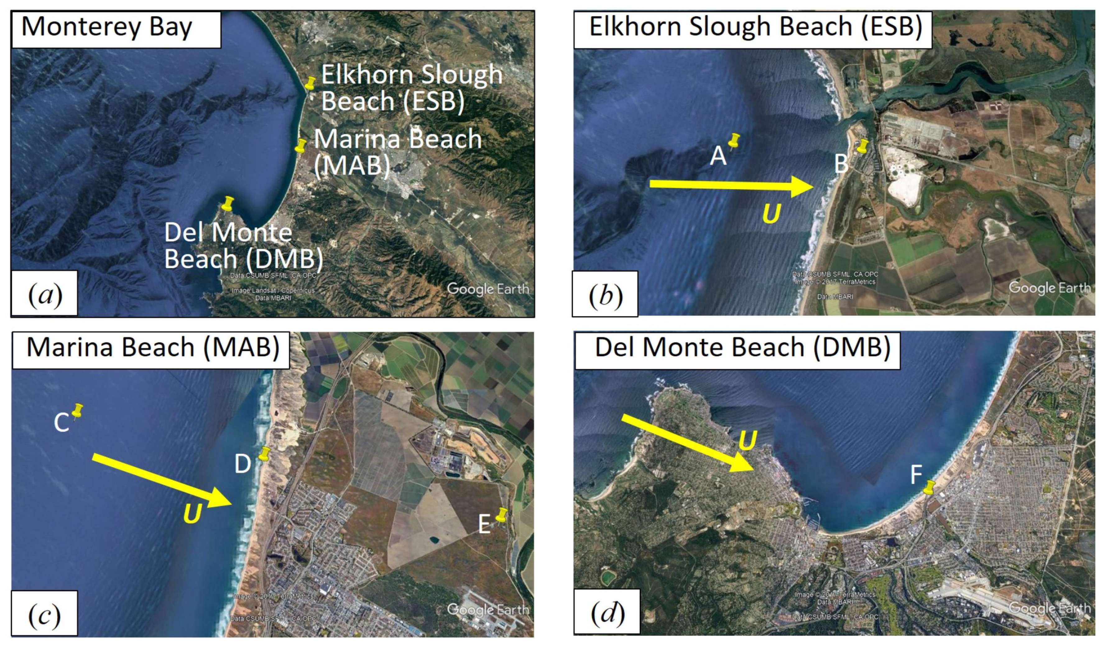
2. Study Cases
3. Numerical Methods
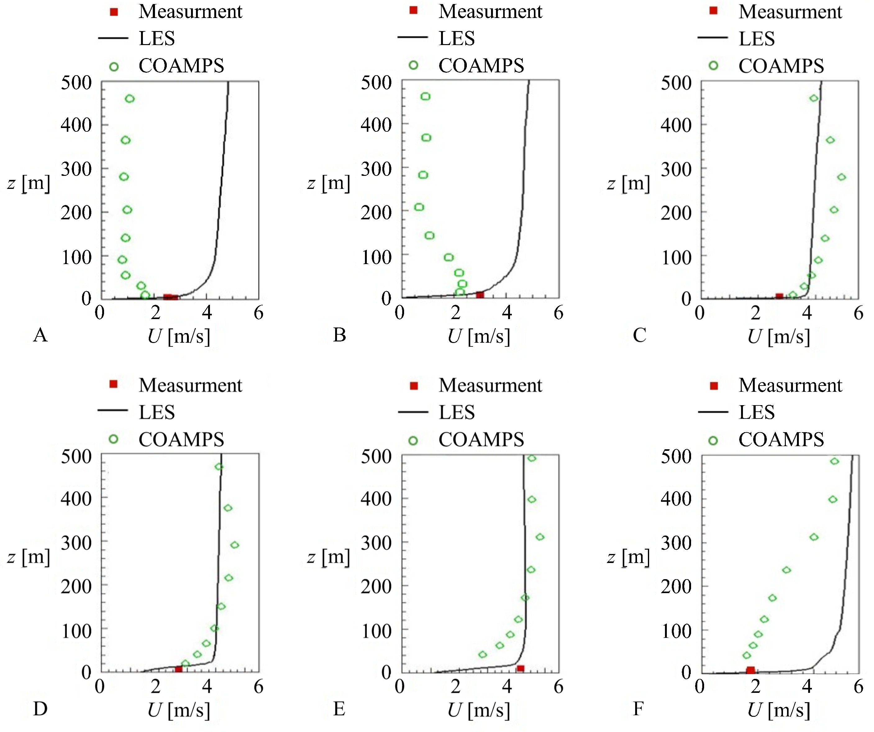
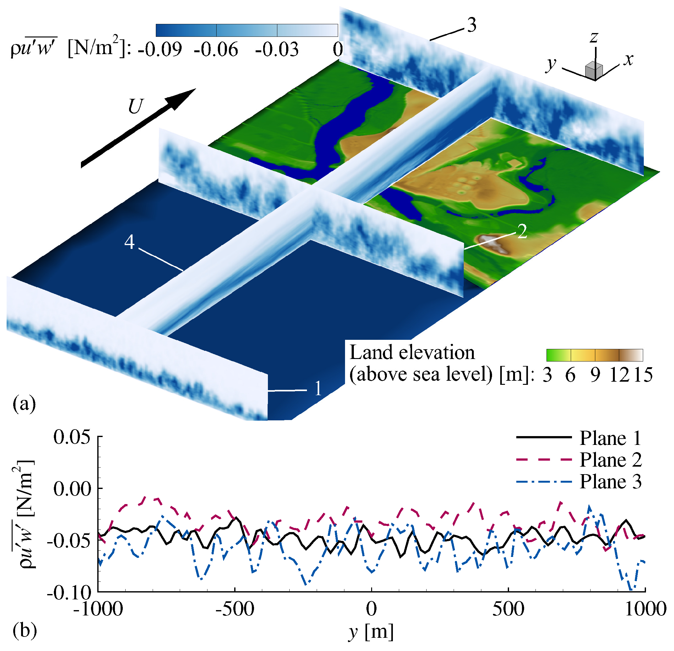
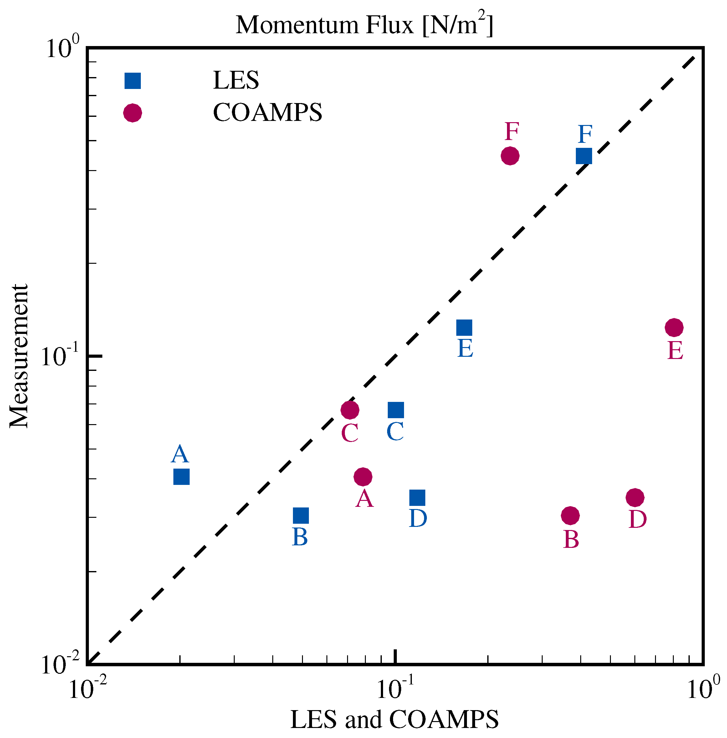
4. Results
5. Conclusions
Acknowledgments
Author Contributions
Conflicts of Interest
Abbreviations
| ABL | Atmospheric boundary layer |
| LES | Large-eddy simulation |
| COAMPS | Coupled Ocean/Atmosphere Mesoscale Prediction System |
| IB | Immersed boundary |
| ESB | Elkhorn Slough Beach |
| MAB | Marina Beach |
| DMB | Del Monte Beach |
| NPS | Naval Postgraduate School |
| UTC | Coordinated universal time |
References
- Shabani, B.; Nielsen, P.; Baldock, T. Direct measurements of wind stress over the surf zone. J. Geophys. Res. Oceans 2014, 119, 2949–2973. [Google Scholar] [CrossRef]
- Ortiz-Suslow, D.G.; Haus, B.K.; William, N.J.; Laxague, N.J.; Reniers, A.J.H.M.; Graber, H.C. The spatial–temporal variability of air–sea momentum fluxes observed at a tidal inlet. J. Geophys. Res. Oceans 2015, 120, 660–676. [Google Scholar] [CrossRef]
- MacMahan, J. Increased aerodynamic roughness owing to surfzone foam. J. Phys. Oceanogr. 2017, 47, 2115–2122. [Google Scholar] [CrossRef]
- Hodur, R.M. The Naval research laboratory’s coupled ocean/atmosphere mesoscale prediction system (COAMPS). Mon. Weather Rev. 1997, 125, 1414–1430. [Google Scholar] [CrossRef]
- Shamarock, W.C.; Klemp, J.B.; Dudhia, J.; Gill, D.O.; Barker, D.M.; Duda, M.G.; Huang, X.-Y.; Wang, W.; Powers, J.G. A description of the advanced research WRF version 3. NCAR Tech. Notes 2008. [Google Scholar] [CrossRef]
- Pielke, R.A.; Cotton, W.R.; Walko, R.L.; Tremback, C.J.; Lyons, W.A.; Grasso, L.D.; Nicholls, M.E.; Moran, M.D.; Wesley, D.A.; Lee, T.J.; et al. A comprehensive meteorological modeling system—RAMS. Meterol. Atmos. Phys. 1992, 49, 69–91. [Google Scholar] [CrossRef]
- Yang, X.; Sotiropoulos, F.; Conzemius, F.; Wachtler, J.N.; Strong, M.B. Large eddy simulation of turbulent flow past wind turbines/farms: The Virtual Wind Simulator (VWiS). Wind Energy 2015, 18, 2025–2045. [Google Scholar] [CrossRef]
- Foti, D.; Yang, X.; Campagnolo, F.; Maniaci, D.; Sotiropoulos, F. On the use of spires for generating inflow conditions with energetic coherent structures in large eddy simulation. J. Turbul. 2017, 18, 611–633. [Google Scholar] [CrossRef]
- Yang, X.; Sotiropoulos, F. A new class of actuator surface models for wind turbines. Wind Energy 2017. [Google Scholar] [CrossRef]
- Lilly, D.K. A proposed modification of the Germano subgridscale closure method. Phys. Fluids A 1992, 4, 633–635. [Google Scholar] [CrossRef]
- Kim, J.; Moin, P. Application of a fractional-step method to incompressible Navier-Stokes equations. J. Comput. Phys. 1985, 59, 308–323. [Google Scholar] [CrossRef]
- Balay, S.; Brown, K.; Eijkhout, V.; Gropp, W.; Kaushik, D.; Knepley, M.; Mcinnes, L.C.; Smith, B.; Zhang, H. PETSc Users Manual Revision 3.3.; Computer Science Division of Argonne National Laboratory: Argonne, IL, USA, 2012. [Google Scholar]
- Ge, L.; Sotiropoulos, F. A numerical method for solving the 3D unsteady incompressible Navier-Stokes equations in curvilinear domains with complex immersed boundaries. J. Comput. Phys. 2007, 225, 1782–1809. [Google Scholar] [CrossRef] [PubMed]
- Calderer, A.; Kang, S.; Sotiropoulos, F. Level set immersed boundary method for coupled simulation of air/water interaction with complex floating structures. J. Comput. Phys. 2014, 277, 201–227. [Google Scholar] [CrossRef]
- Mittal, R.; Gianluca, I. Immersed boundary methods. Annu. Rev. Fluid Mech. 2005, 37, 239–261. [Google Scholar] [CrossRef]
- Kang, S.; Sotiropoulos, F. Flow phenomena and mechanisms in a field-scale experimental meandering channel with a pool-riffle sequence: Insights gained via numerical simulation. J. Geophys. Res. 2011, 116, F03011. [Google Scholar] [CrossRef]
- Escauriaza, C.; Sotiropoulos, F. Initial stages of erosion and bed-form development in turbulent flow past a bridge pier. J. Geophys. Res. 2011, 116, F03007. [Google Scholar] [CrossRef]
- Khosronejad, A.; Kang, S.; Borazjani, I.; Sotiropoulos, F. Curvilinear immersed boundary method for simulating coupled flow and bed morphodynamic interactions due to sediment transport phenomena. Adv. Water Resour. 2015, 34, 829–843. [Google Scholar] [CrossRef]
- Calderer, A.; Guo, X.; Shen, L.; Sotiropoulos, F. Coupled fluid–structure interaction simulation of floating offshore wind turbines and waves: A large eddy simulation approach. J. Phys. Conf. Ser. 2014, 524, 012091. [Google Scholar] [CrossRef]
- Charnock, H. Wind stress on a water surface. Q. J. R. Meteorol. Soc. 1955, 81, 639–640. [Google Scholar] [CrossRef]
- Mann, J. Wind field simulation. Probab. Eng. Mech. 1998, 13, 269–282. [Google Scholar] [CrossRef]
- Mann, J. The spatial structure of neutral atmospheric surface-layer turbulence. J. Fluid Mech. 1994, 273, 141–168. [Google Scholar] [CrossRef]
- Hogan, T.F.; Liu, M.; Ridout, J.A.; Peng, M.S.; Whitcomb, T.R.; Ruston, B.C.; Reynolds, C.A.; Eckermann, S.D.; Moskaitis, J.R.; Baker, N.L.; et al. The navy global environmental model. Oceanography 2014, 27, 116–125. [Google Scholar] [CrossRef]
- Mellor, G.; Yamada, T. Development of a turbulence closure model for geophysical fluid problems. Rev. Geophys. 1982, 20, 851–875. [Google Scholar] [CrossRef]
- Louis, J.F. A parametric model of vertical eddy fluxes in the atmosphere. Bound. Layer Meteorol. 1979, 17, 187–202. [Google Scholar] [CrossRef]
- Wang, S.; Wang, Q.; Doyle, J. Some improvement of Louis surface flux parametrization. In Proceedings of the 15th Symposium on Boundary Layer and Turbulence, Wageningen, The Netherlands, 15–19 July 2002; pp. 547–550. [Google Scholar]
- Blackadar, A.K. The vertical distribution of wind and turbulent exchange in a neutral atmosphere. J. Geophys. Res. 1962, 67, 3095–3102. [Google Scholar] [CrossRef]
- Hodur, R.M.; Jakubiak, B. The effect of the physical parameterizations and the land surface on rainfall in Poland. Weather Forecast. 2016, 31, 1247–1270. [Google Scholar] [CrossRef]
- Perlin, N.; de Szoeke, S.P.; Chelton, D.B.; Samelson, R.M.; Skyllingstad, E.D.; O’Neill, L.W. Modeling the atmospheric boundary layer wind response to mesoscale sea surface temperature perturbations. Mon. Weather Rev. 2014, 142, 4284–4307. [Google Scholar] [CrossRef]
- Wang, S.; O’Neill, L.W.; Jiang, Q.; de Szoeke, S.P.; Hong, X.; Jin, H.; Thompson, W.T.; Zheng, X. A regional real-time forecast of marine boundary layers during VOCALS-REx. Atmos. Chem. Phys. 2011, 11, 421–437. [Google Scholar] [CrossRef] [Green Version]
- Fröhlich, J.; Mellen, C.P.; Rodi, W.; Temmerman, L.; Leschziner, M.A. Highly resolved large-eddy simulation of separated flow in a channel with streamwise periodic constrictions. J. Fluid Mech. 2005, 526, 19–66. [Google Scholar] [CrossRef]
- Breuer, M.; Peller, N.; Rapp, C.; Manhart, M. Flow over periodic hills—Numerical and experimental study in a wide range of Reynolds numbers. Comput. Fluids 2009, 38, 433–457. [Google Scholar] [CrossRef]
- Rasam, A.; Wallin, S.; Brethouwer, G.; Johansson, A.V. Large eddy simulation of channel flow with and without periodic constrictions using the explicit algebraic subgrid-scale model. J. Turbul. 2014, 15, 1–24. [Google Scholar] [CrossRef]
- Le, H.; Moin, P.; Kim, J. Direct numerical simulation of turbulent flow over a backward-facing step. J. Fluid Mech. 1997, 330, 349–374. [Google Scholar] [CrossRef]
- Fang, X.; Yang, Z.; Wang, B.-C.; Tachie, M.F.; Bergstrom, D.J. Highly-disturbed turbulent flow in a square channel with V-shaped ribs on one wall. Int. J. Heat Fluid Flow 2015, 56, 182–197. [Google Scholar] [CrossRef]
- Fang, X.; Yang, Z.; Wang, B.-C.; Tachie, M.F.; Bergstrom, D.J. Large-eddy simulation of turbulent flow and structures in a square duct roughened with perpendicular and V-shaped ribs. Phys. Fluids 2017, 29, 065110. [Google Scholar] [CrossRef]


| Real-Time Cases | ||
|---|---|---|
| Case | Location | Date and Time (UTC) |
| ESB1 | Elkhorn Slough Beach (Figure 1b) | 15 June 2016, 17:00 |
| MAB | Marina Beach (Figure 1c) | 13 June 2016, 17:20 |
| DMB | Del Monte Beach (Figure 1d) | 12 June 2016, 23:00 |
| What-If Cases | ||
| Case | Location | Setup |
| ESB2 | inlet wind speed of case ESB1 | |
| ESB3 | inlet wind speed of case ESB1 | |
| ESB4 | Elkhorn Slough Beach (Figure 1b) | inlet wind speed of case ESB1 |
| ESB5 | Offshore wind with the same inlet wind speed of case ESB1 | |
| ESB6 | Flat land topography with the same inlet wind speed of case ESB1 | |
© 2018 by the authors. Licensee MDPI, Basel, Switzerland. This article is an open access article distributed under the terms and conditions of the Creative Commons Attribution (CC BY) license (http://creativecommons.org/licenses/by/4.0/).
Share and Cite
Yang, Z.; Calderer, A.; He, S.; Sotiropoulos, F.; Doyle, J.D.; Flagg, D.D.; MacMahan, J.; Wang, Q.; Haus, B.K.; Graber, H.C.; et al. Numerical Study on the Effect of Air–Sea–Land Interaction on the Atmospheric Boundary Layer in Coastal Area. Atmosphere 2018, 9, 51. https://doi.org/10.3390/atmos9020051
Yang Z, Calderer A, He S, Sotiropoulos F, Doyle JD, Flagg DD, MacMahan J, Wang Q, Haus BK, Graber HC, et al. Numerical Study on the Effect of Air–Sea–Land Interaction on the Atmospheric Boundary Layer in Coastal Area. Atmosphere. 2018; 9(2):51. https://doi.org/10.3390/atmos9020051
Chicago/Turabian StyleYang, Zixuan, Antoni Calderer, Sida He, Fotis Sotiropoulos, James D. Doyle, David D. Flagg, Jamie MacMahan, Qing Wang, Brian K. Haus, Hans C. Graber, and et al. 2018. "Numerical Study on the Effect of Air–Sea–Land Interaction on the Atmospheric Boundary Layer in Coastal Area" Atmosphere 9, no. 2: 51. https://doi.org/10.3390/atmos9020051