Assembling Typical Meteorological Year Data Sets for Building Energy Performance Using Reanalysis and Satellite-Based Data

Joint Research Centre, European Commission, Via Fermi, 2749, I-21027 Ispra, Italy
*
Author to whom correspondence should be addressed.
Atmosphere 2018, 9(2), 53; https://doi.org/10.3390/atmos9020053
Submission received: 9 January 2018
/
Revised: 25 January 2018
/
Accepted: 31 January 2018
/
Published: 6 February 2018
(This article belongs to the Special Issue Energy Meteorology)
Abstract
:We present a method to generate Typical Meteorological Year (TMY) data sets for use in calculations of the energy performance of buildings, based on satellite derived solar radiation data and other meteorological parameters obtained from reanalysis products. The great advantage of this method is the availability of data over large geographical regions, giving global coverage for the reanalysis and continental-scale coverage for the solar radiation data, making it possible to generate TMY data for nearly any location, independent of the availability of meteorological measurement stations in the area. The TMY data generated with this method have been validated against 487 meteorological stations in Europe, by calculating heating and cooling degree days, and by running building energy performance simulations using EnergyPlus. Results show that the generated data sets using a long time series perform better than the TMY data generated from station measurements for building heating calculations and nearly as well for cooling calculations, with relative standard deviations remaining below 6% for heating calculations. TMY data constructed using the proposed method yield somewhat larger deviations compared to TMY data constructed from station data. We outline a number of possibilities for further improvement using data sets that will become available in the near future.
1. Introduction
Climatic data are essential in order to calculate the heating or cooling requirements of new or refurbished buildings. Often these data are used in the form of a Typical Meteorological Year (TMY). The first TMY data set was produced for 248 locations in the United States by Sandia National Laboratories [1], using long-term weather and solar data collected for the period 1952–1975. In 1994, the TMY data have been updated (as TMY2) by the National Renewable Energy Laboratory (NREL) using data covering the period 1961–1990 [2]. The latest release of TMY3 is based on input data for 1976–2005 [3].
In Europe, several reference climatic data sets have also been generated, but in a less harmonised way. For instance [4]:
- In Italy, the climatic data collection “Gianni De Giorgio” (IGDG) (a set of 66 climatic data sets is based on a 1951–1970 period of record) was developed for use in simulating renewable energy technologies.
- The Spanish Weather for Energy Calculations (SWEC) were generated to cover all 52 Spanish provincial capitals.
- The IMGW weather data set for Poland (Instytut Meteorologii i Gospodarki Wodnej) includes 61 climatic data sets developed by the Polish Ministry of Infrastructure.
The overall availability of TMY data is thus heterogeneous and the geographical distribution varies strongly.
TMY data sets consist of one year of climatic data selected from a long time series of data spanning many years (normally 10 or more). The TMY is constructed by choosing data for each month from different years so that the data for a given month is the most “typical” among the years present in the long-term data set. One way to construct the TMY is described in the International Standard ISO 15927-4 [5].
Calculating the energy performance of buildings requires a large number of climatic variables. Some of these, such as temperature, pressure and relative humidity, are measured at many sites. Others are rarer, such as global horizontal solar radiation, while some again are measured only at few sites in the world. Illuminance, thermal infrared radiation from the sky or direct normal solar radiation fall into this group. These constraints are evident even in recent works such as that of Kim et al. [6] in which ISO 15927-4 is used to construct TMY data for Korea, but where the number of stations with solar radiation data is much lower than the number of measurement stations providing the more traditional meteorological variables.
Even though some of the necessary parameters (e.g., temperature, pressure, wind speed) are measured at a large number of stations in the world, there are large areas of the world where data coverage is very sparse. In addition, not all these data are freely available, so getting the necessary data for a particular location may be difficult [7].
In order to deal with missing data, the software packages for energy performance calculations of buildings often have built-in models to estimate the missing parameters. However, it will of course be an advantage if the data are directly available. For instance, Bojanowski et al. [8] found that models of solar radiation have lower accuracy than satellite-based solar radiation products.
In recent years, a number of data sets have become freely available that estimate solar radiation from satellite data [9,10,11,12]. Using images from geostationary satellites, these data sets provide solar radiation values with a spatial resolution of a few km and hourly temporal resolution (sometimes even higher). In this way, solar radiation data are now available at any location over large geographical areas for long time periods (up to 30 years at present in some areas [12]).
Climatic data can now also be obtained at a global scale from a number of reanalysis data sets, which use computational meteorological forecast models to recalculate the weather forecast output corrected with data from meteorological stations. These data sets typically have high temporal resolution (1–3 h) and contain long time series, but generally the spatial resolution is quite low. For the ERA-interim data set [13] of the European Centre for Medium-Range Weather Forecast (ECMWF) [14], the resolution is in latitude and longitude (about 80 km). NASA’s MERRA-2 [15] reanalysis uses a spatial resolution of . These data sets contain all the usual climatic parameters measured at meteorological stations and in addition a large number of parameters, including incoming solar radiation and downwelling thermal infrared radiation, which are useful for building energy performance studies.
The widespread availability of these data makes it worthwhile to investigate whether they can be used as input to building energy performance studies. Here, we will present a method to generate TMY data from satellite-based solar radiation data and reanalysis climate data. The method has been validated against data from meteorological stations in Europe.
The advantages of this new method are twofold: it provides data at any location over large geographical areas, including regions with only few or no measurements at all. In addition, it provides solar radiation data that are normally difficult to obtain.
The paper is organized as follows: Section 2 describes the data used to construct TMY data sets, either from reanalysis data or from ground station measurements. Section 3 presents the criteria used to select ground stations and methods for reconstructing missing data values. Section 4 describes the validation that has been performed to assess the quality of the reanalysis-based TMY data sets. Finally, we present conclusions and future work in Section 5.
The methods described in this paper have been implemented as a web application and web service, available here:
http://re.jrc.ec.europa.eu/tmy.html.
The TMY generator has also been implemented as part of the PVGIS online solar radiation and photovoltaic energy estimation tool in the new version 5 of PVGIS:
http://re.jrc.ec.europa.eu/pvg_tools/en/tools.html.
At the time of writing, the web application will produce only TMY data, i.e., one year of hourly climatic data. However, in the future, it will also be possible to download a longer time series of the same climatic quantities.
2. Data Sources
2.1. Solar Radiation Data
Hourly values of global horizontal and direct normal irradiance are available at a spatial resolution of 4 km from the CM SAF collaboration [16], based on satellite data. The methods and validation are described in Müller et al. [9] and Gracia Amillo et al. [10]. Data are available for an area covering Europe as far north as N, Africa, parts of South America (to W) as well as most of Asia to about E [10]. In addition, the online TMY generator uses data from the National Solar Radiation Database [11] to cover North America to N and parts of South America. However, these data have not been used in the validation of the method.
The methods for generating TMY data described here should be usable also with solar radiation data from other geostationary satellites.
Local shadows from terrain (hills or mountains) may significantly influence the amount of solar radiation arriving at a given location. In this work, we have used data from the Shuttle Radar Topography Mission (SRTM-3) digital elevation model data [17] to calculate the horizon height around each location and from that calculate the attenuation of the direct solar irradiance [18].
2.2. Ground Station Measurement Data
A large part of the ground station data used for this study has been downloaded from the NOAA Integrated Surface Database (ISD) archive [19]. From the stations available at this site, we selected the stations in Europe for which data are available from 2005 onwards.
The ISD-lite data contain the following quantities:
- Air temperature at 2 m above ground,
- Dewpoint temperature at 2 m above ground,
- Wind speed at 10 m,
- Wind direction,
- Pressure,
- Precipitation and sky cover data not used for the present study.
In addition to the ISD data, we have used ground station data from the German Weather Service DWD, whose data are available at the DWD Climate Data Center:
http://www.dwd.de/EN/climate_environment/cdc/cdc_node.html.
The meteorological quantities used from these data are the same as for the NOAA ISD data except that these data report the relative humidity instead of the dewpoint temperature.
2.3. Reanalysis Data
The European Centre for Medium-range Weather Forecast (ECMWF) [14] makes available the “ERA-interim” reanalysis data set [13]. The data have global coverage with a temporal resolution of 3 h and a spatial resolution of latitude/longitude. Among the very large number of physical quantities in the data the ones used for this study are:
- Air temperature at 2 m above ground
- Dewpoint temperature at 2 m above ground
- Wind speed at 10 m (calculated from the two wind speed components)
- Wind direction
- Air pressure
- Surface downward thermal infrared irradiance
Due to the coarse spatial resolution, the temperature data may especially become very inaccurate in areas with large elevation differences. To overcome this problem, we have employed a vertical temperature downscaling procedure (see [20] for a description of the method as well as extensive validation of the uncorrected and corrected ERA-interim air temperature data).
Hourly data are produced from the 3-h ERA-interim data by linear interpolation of each data field.
3. Input Data Preparation
3.1. Selection of Ground Station Data
While the ISD station database contains a very large number of meteorological stations, many of these have large gaps in the time series, making them unsuitable for use as input to building energy performance calculations.
The first step in the selection of ground stations was to require that at least 85,000 values be present for all the necessary fields, out of the 87,648 h in the time period. The only exception to this is that the air pressure allowed for having more missing values since the effect of varying pressure on building energy performance is quite weak.
3.2. Data Gap Filling
While the reanalysis data have complete time series, the solar radiation data and the ground station data have cases of missing values. In order to produce a complete data set, some gap-filling must be performed.
3.2.1. Gap Filling of the Solar Radiation Data
For the solar radiation data, a total of 85,079 h were available out of 87,648 or about 97%. Since the solar irradiance values naturally vary strongly during the day, it makes little sense to perform a simple interpolation. The method used to fill the gaps has therefore been chosen as follows: calculate the missing hour as the average of the same hour in the year for all the other years (so, for instance, 23 January 2009 at 4:00 p.m. would be calculated as the average of 23 January at 4:00 p.m. from all the other years).
3.2.2. Gap Filling of the Meteorological Station Data
For the station data, periods with missing data are filled by linear interpolation between the last hour before the gap to the first hour after the gap.
In a few cases, this may lead to an unrealistic time series when the interpolation is performed over a longer time interval. However, in this case, the month that includes this unrealistic interval will almost certainly be excluded by the TMY selection algorithm because the probability density functions of the climatic variables will be far from the normal shape (see Section 3.3).
3.3. Construction of Typical Meteorological Years
The procedure to construct Typical Meteorological Years (TMY) follows the ISO 15927-4 [5] standard. For each month in the year, the data are taken from the year calculated as most “typical” for that month. The Standard specifies the method to construct the TMY based on a statistical evaluation of air temperature, relative humidity and solar radiation, with a less important contribution from the wind speed data. A brief summary of the procedure is given here:
- For each of the three quantities (air temperature, relative humidity and solar radiation), calculate the daily means from the hourly values.
- For each quantity q and each month m, calculate the cumulative distribution function using all the daily values for all years.
- For each quantity q, each year y and each month m, calculate the cumulative distribution function using all the daily values for that year.
- For each q, m and y, calculate the Finkelstein–Schafer statistic, summing over the range of the distribution values:
- For each m and q, rank the the individual months in the multi-year period in order of increasing
- For each m and y, add the ranks for the three quantities.
- For each m, for the three months with the lowest total ranking, calculate the deviation of the monthly average wind speed from the multi-year mean for that month. The lowest deviation in wind speed is used to select the “best” month to be included in the TMY.
The metric used to assess similarity is the cumulative distribution function for each of the meteorological quantities.
The primary application of the data generated by the method described here is building energy performance calculations, which is also the scope of ISO-15927-4. The ISO-15927-4 method prescribes an equal weight to air temperature, solar radiation, and relative humidity, when selecting the typical months. However, this may not be optimal for all applications. For instance, methods have been developed to generate TMY specifically for solar energy applications [21,22].
The Standard is somewhat unclear as to the way the different solar radiation components are to be included in the calculations to construct the TMY. While the quantities to be supplied include both global horizontal and direct normal irradiance, the selection of the typical months is to be based on the “solar radiation”, but it is not specified if both components have to be used or with what weighting. In the following, we have used only the global horizontal irradiance component in the construction of the TMY.
The Standard also specifies that the boundaries between the months (8 h at the end of one month and 8 at the beginning of the next) should be smoothed by interpolation. This has been done for all fields except solar radiation where such an interpolation across night hours would not make sense (This choice may have to be revised if the method is used in regions where UTC midnight happens during the daytime).
The output formats of the TMY data files are described in Appendix A.
4. Validation
The purpose of the validation is to quantify the difference when using reanalysis data instead of station data for the construction of the TMY. Some of the data used in the TMY will in any case be the same. This is the case for the solar radiation components (global horizontal and direct normal irradiance), which are always derived from satellite data because of the scarceness of measured data (even here, the solar radiation data in the TMY data sets may differ because the methods may choose different years when processing the station data or the reanalysis data). In the same way, the thermal (long-wave) infrared irradiance is always taken from the reanalysis data, again because ground station measurements are extremely rare. This means that the comparison will be done based on the difference between station data and reanalysis data in the following quantities:
- Dry bulb temperature (2 m temperature) (C),
- Wind speed (m/s),
- Wind direction (degrees clockwise from north),
- Relative humidity (-),
- Air pressure (Pa).
4.1. Data Sets for the Validation
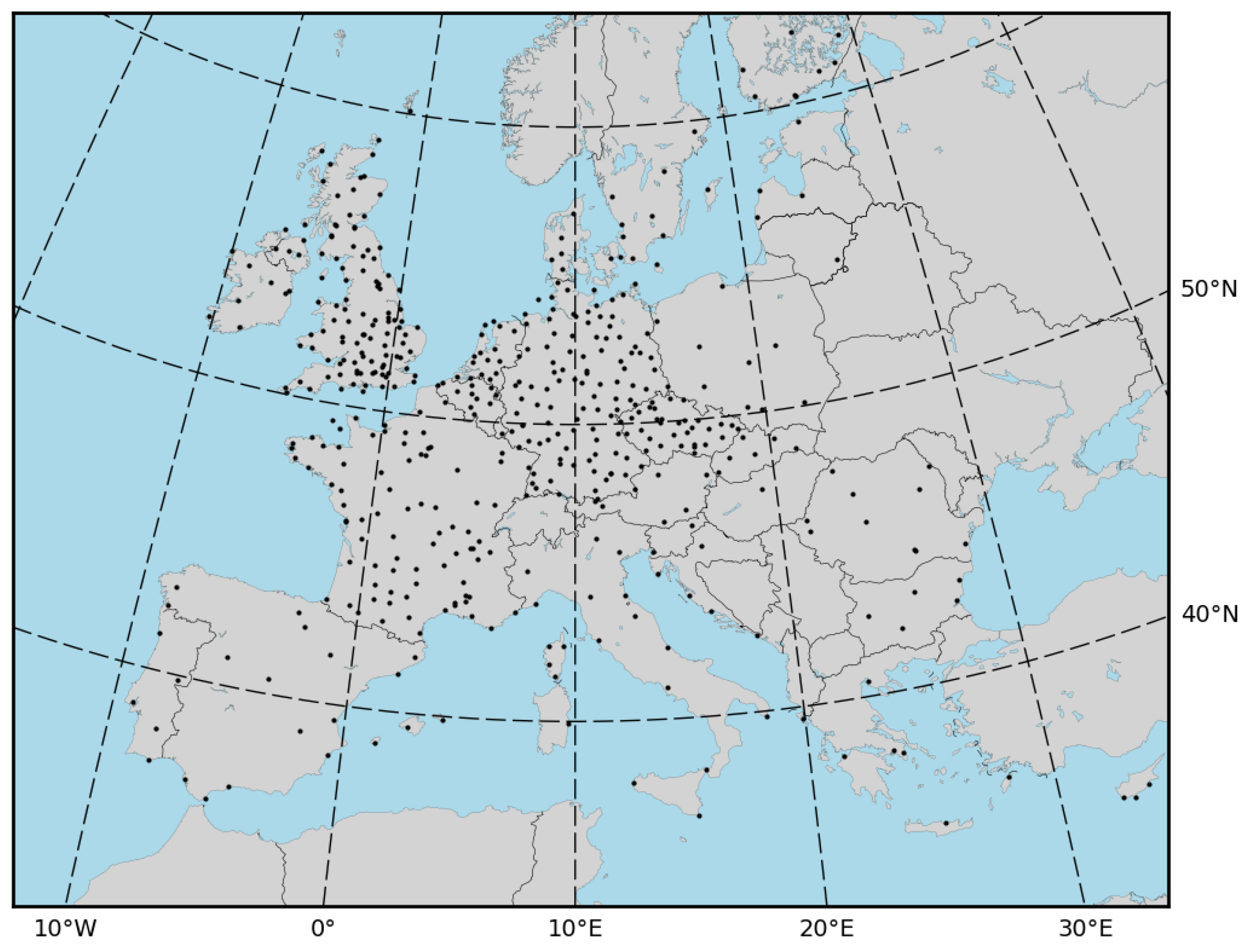
The data sets used for the validation consist of the ground station data for 490 locations (390 taken from ISD-lite and 100 obtained from DWD) for the time period 2005–2014. For each of the station locations, the same time interval has been used to construct data sets using the reanalysis data. The locations of the ground stations are shown in Figure 1.
The main aim of the validation is to compare the TMY data sets generated with the ground station data against those made with the reanalysis data. However, the generation of the TMY will itself cause a deviation from the results you would get when using the full multi-year data set. For this reason, we will compare the results from four different data sets:
- 10 years of hourly data using ground station data,
- 10 years of hourly data using reanalysis data,
- TMY data generated using ground station data,
- TMY data generated using reanalysis data.
In this list, the first data set will be taken as a reference, and the results using the other data will be compared to this.
4.2. Validation Metrics
The input data used to construct the TMY data sets have been validated in a number of studies, as noted in the description in Section 2. For the present study, we have therefore chosen to use as validation the output of calculations using the data sets. The TMY data sets are intended for use in building energy performance calculations. Hence, we have chosen the following two metrics:
- Heating and cooling degree days,
- Heating and cooling energy loads for buildings, calculated using a well-known software for simulating building energy performance.
The advantage of this approach is that it informs the user of the data sets about the likely deviations that result from using these data sets instead of other approaches.
4.2.1. Degree Days
Degree days is a rather simple measure of how much heating or cooling will be necessary over a time period consisting of many days. Degree days are used here only as a way to compare different data sets; the precise values will depend on the method used to calculate the degree days. There is no universal standard for how to calculate degree days. We have used the following definitions, which are also used by EUROSTAT [23]:
Heating Degree Days (HDD) are calculated for a given day with average dry-bulb temperature as:
The total HDD for a given period is then calculated by summing of the individual days:
In a similar way, the cooling degree days are calculated as:
In the following, HDD and CDD will be calculated per year (yearly averages for the long time series and a single value for the TMY).
4.2.2. Simulations with EnergyPlus
Degree days are a rather coarse way of estimating heating/cooling energy requirements. A better way would be to perform an actual simulation of the energy performance of a building in each of the station locations.
To simulate energy performance for buildings, we have used the EnergyPlus software [24]. EnergyPlus is an open-source software funded by the Building Technologies Office of the U.S. Department of Energy. EnergyPlus can calculate heating/cooling loads for buildings given the necessary input building parameters and a climatic data set in the form of a TMY data sets for the given location.
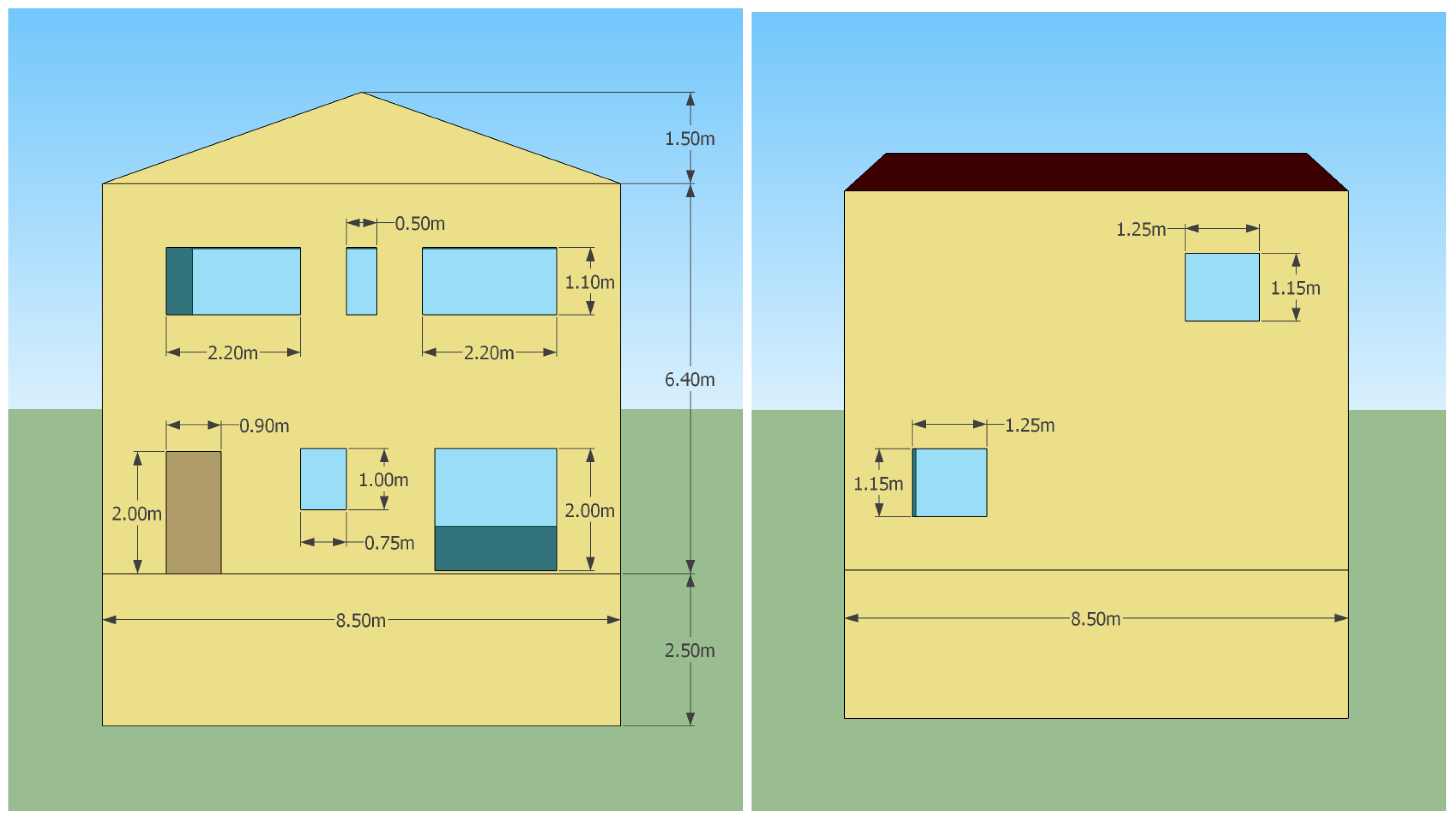
For this study, EnergyPlus (version 8.7) has been used to perform dynamic simulations of heating and cooling for buildings. Two relatively simple building configurations have been used with the climatic data for all 487 locations in order to quantify the difference in the performance estimate using the different data sources.
Since the simulation will have to be performed a few thousand times, simplified models of buildings have been defined and used for the simulations. The primary simplification is that the design consists of a single thermal zone. One design is of a small building (a single family house), composed of two conditioned floors over the ground level and an unconditioned under-ground level. The surface is about 140 and the ratio between all dispersing surface and heated/cooled volume (S/V ratio) is 0.7.
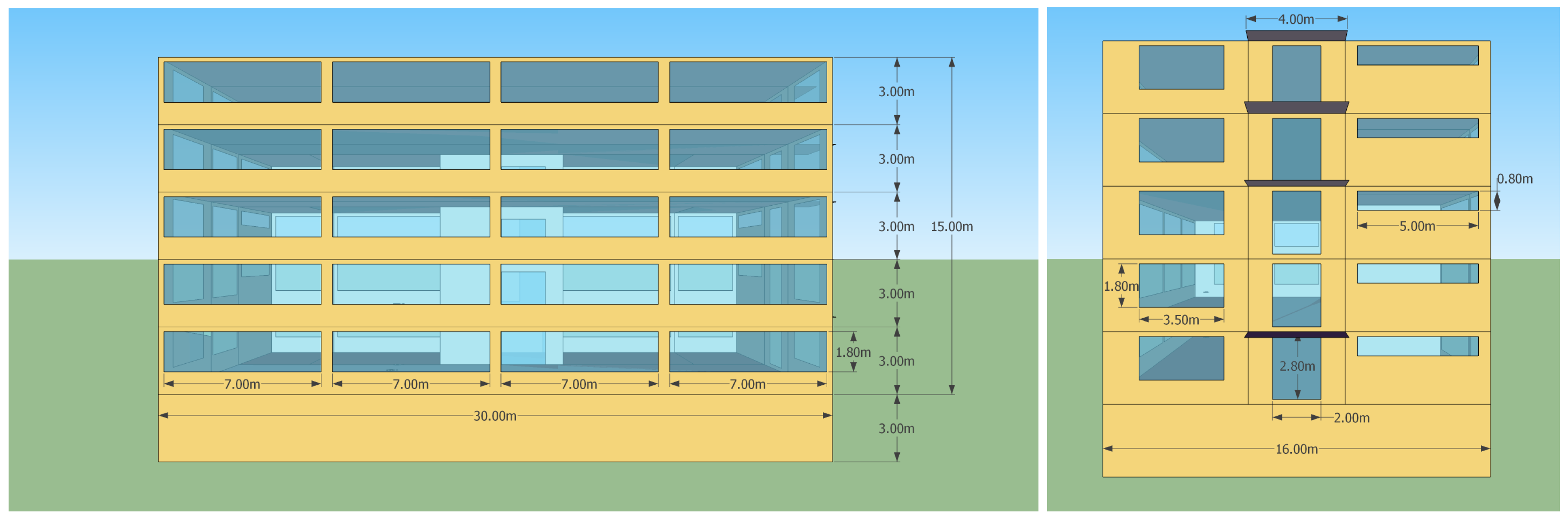
The other building design is for a larger building designed for office use. This is a medium-size and highly-glazed building with five floors (of 3 m height each), an S/V ratio of 0.33 and a net heated area of 2400 . Because of the larger solar and internal gains, this model is exposed to greater energy demand for cooling compared to the house.
The models used represent typical existing buildings built in 1960–1970s, with an uninsulated envelope (U-values of opaque elements between 1.2 and 1.7 ) and simple double-pane windows (U-value of 3.0 ).
The main other characteristics involved on the simulation task are given in Table 1. The layouts of the building models are shown in Figure 2 and Figure 3.
The output of the EnergyPlus calculation consists of the hourly total energy needs for space heating and cooling, for sensible and latent energy loads. For the purposes of validation, only the yearly total heating and cooling energy demand will be considered.
4.3. Statistical Quantities
For each station, there will be a difference between the calculations performed with the full time series of the station data and the calculations using the other data sets. The following summary statistics will be performed: let be the heating degree days for the i-th station location using the full station data set, using the full reanalysis data, using the station derived TMY data set, and calculated from the reanalysis-based TMY data. Then, we can calculate the Mean Absolute Deviation (MAD) between, say, HDD from station TMY data and HDD from full station data as:
Similarly, the standard deviation can be calculated as:
The statistics of differences between other combinations of data sets are calculated in a similar way. For instance, the MAD between HDD calculated with station data and ERA data can be expressed as:
4.4. Validation Results
In the end, there will be four quantities to examine:
- Heating degree days HDD (-),
- Cooling degree days CDD (-),
- Heating energy requirements (kWh/) for each building,
- Cooling energy requirements (kWh/) for each building.
- Full reanalysis data set against full station data set,
- Station-based TMY against full station data set,
- Reanalysis-based TMY against full station data set,
- Reanalysis-based TMY against station-based TMY.
4.4.1. Degree Days
The summary statistics for the degree days calculation are shown in Table 2.
Since a large number of stations in the sample have low values of cooling degree days, the statistics for these quantities have not been done on all stations. For CDD, only stations with CDD > 50 have been used for the statistics, which leaves 99 stations for the analysis.
4.4.2. Energy Consumption, Single Family House
The statistics for the single-family house energy consumption are given in Table 3.
Since a large number of stations in the sample have low values of cooling energy requirements, the statistics for these quantities have not been done on all stations. For the cooling energy consumption, stations have been included if the annual cooling energy consumption is . This criterion is satisfied by 101 stations.
The pattern of results is quite similar between the degree days calculation and the energy consumption estimates. For heating and HDD, the deviations found when comparing the full station data with the full ERA data set are slightly smaller than the deviations between full station data and station TMY data, though the difference is not statistically significant (F-distribution test). For cooling, the smallest deviation is seen when comparing the full station data to the station-based TMY, while the comparison of full station against full ERA data yields deviations that are somewhat larger (statistically significant at >99%). The deviation between the full station data and the ERA TMY is somewhat larger again, while the largest deviation is found between station-based TMY and ERA TMY.
The statistical measures shown above do not give an indication of any geographical variation in the deviations. To show this, we have plotted the the difference in energy consumption estimates between the full ERA and full station data sets (Figure 4), and the difference when using the station-based TMY and full station data (Figure 5).
Interestingly, the full ERA-based data performs better than the station TMY in many areas including large parts of Central Europe. On the other hand, there are a number of locations where the deviation is large. The number of these locations is rather low and therefore it is difficult to identify a clear pattern.
The comparison between the ERA-based TMY and the station TMY is shown in Figure 6 for both heating and cooling. Since the cooling requirements for the single-family house are much lower than the heating requirements in nearly all areas, it is not surprising that also the deviations are much smaller.
The map of differences in the heating requirements shows a similar pattern to those of Figure 4, but the differences are generally larger, in agreement with the results shown in Table 3.
The maps in Figure 4, Figure 5 and Figure 6 show the absolute difference between the different energy consumption calculations. For illustration, we have also plotted the relative differences in Figure 7 corresponding to Figure 4 (difference between full ERA and full station data). The map shows that, while the absolute differences do not show a strong geographical pattern, the relative differences tend to be larger in the south. This is not surprising, since the overall heating loads in these areas are low, so any uncertainty will tend to inflate the relative differences.
The maps in Figure 4, Figure 5, Figure 6 and Figure 7 show that the deviations when using the TMY data can be quite large in some locations while other locations have very small deviations. In order to study the reasons for this variation, we have calculated the probability density function (PDF) for air temperature for two locations: one in western France (45.683 N, 0.318 W), and one on the coast of Cyprus (34.875 N, 33.625 E). The former has low relative difference in calculated heating loads (+3.5%), while the latter shows a large relative difference in heating load (−20.5%) (comparing station TMY to ERA TMY). The plots in Figure 8 show the PDF for the full station data, the station-based TMY, and the ERA-based TMY.
For the case with low deviation in heating loads, there is no really clear pattern in the differences between the PDFs of the full station data and the two TMY data sets, though the ERA-based TMY tends to slightly underestimate the probability of high temperatures. On the other hand, the case from Cyprus shows a quite strong underestimation of the probabilities of both very low and very high temperatures in the ERA-based TMY. This leads to underestimating both heating and cooling loads for this location. This site is on the coastline of the Mediterranean, where there tends to be large temperature differences between land and sea, with the sea being warmer than land in winter and colder than land in summer.
Another way to compare the probability density functions of the data is to look at the Kolmogorov–Smirnov (KS) statistics. We have calculated the KS-statistic of air temperature for each station location comparing the full 10-year time series of station data with the corresponding 10-year reanalysis data. In order to compare these results with the energy consumption calculations from EnergyPlus, we have looked only at the three winter months December–January–February, and compared these with the heating requirements. Figure 9 shows the difference in heating requirements (using 10-year reanalysis versus the 10-year station data) against the KS-statistic for each location.
For most stations, the KS-statistic value lies between 0.15 and 0.25, and the heating requirement difference shows both negative and positive values in this range. For larger KS values, the difference tends to be negative (heating underestimated when using reanalysis data), but it is difficult to make any firm conclusions from these results. Some of the largest differences in the heating requirements calculation occur when the KS statistic has relatively small values.
4.4.3. Validation Results, Office Building
For this building configuration, we have compared only the station TMY against the ERA TMY results. Again, here we show the average and the statistical measures per . The results are given in Table 4. In this case, nearly all cases (451 out of 487) had a cooling load greater than 2 , and, therefore, all sites have been kept in the statistical treatment. The differences have been plotted in Figure 10.
Compared to the single-household building, the heating requirements per are considerably lower, but, on the other hand, the cooling requirements are higher and, at nearly all sites, some cooling is needed.
The maps in Figure 6, Figure 7, Figure 8, Figure 9 and Figure 10 show that, while most sites show only small differences in heating or cooling loads, there are a few sites that show large deviations. There are some indications from the maps that several of the sites with large deviations in cooling loads are located close to the sea, especially in Southern Europe. A possible reason for these deviations could be that the ERA data used inland close to the coast actually represent areas over the sea, where the temperature can be quite different from land temperatures. The downscaling procedure for the temperature may not always be sufficient to account for this effect.
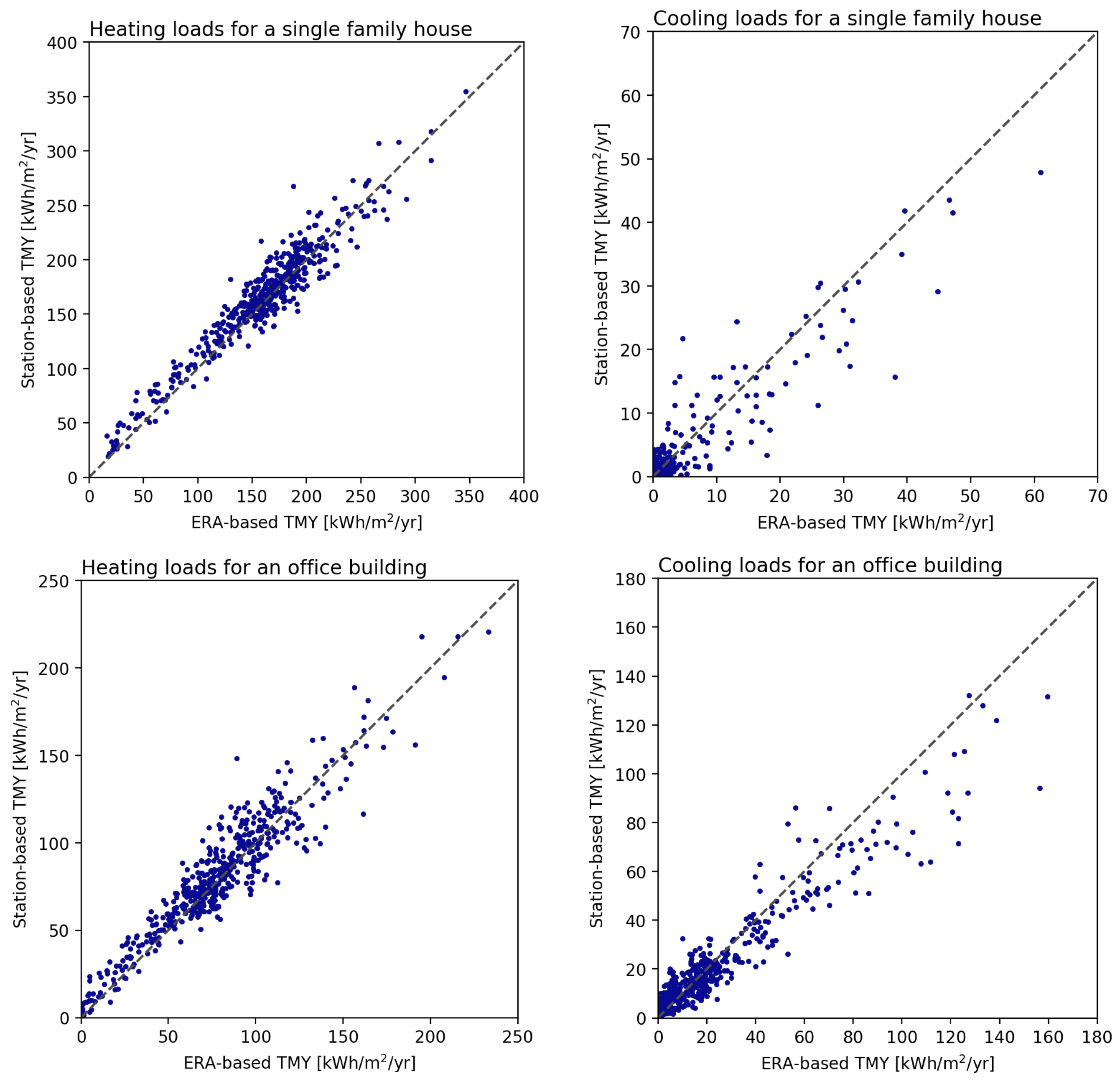
Figure 11 presents a comparison between the station-based TMY and the ERA-based TMY results as scatterplots of the deviation between EnergyPlus calculation results using the two sets of TMY data. The results are shown for the two building configurations (house and office building), for both heating and cooling.
The plots show larger scatter for the cooling loads than for heating. In particular for the single-family house, the cooling loads show a very large scatter, which however is related to the fact that the overall cooling energy requirements are low.
4.4.4. Additional Comparisons, Single-Family House
For the calculations using the single-family house configuration, we performed two extra sets of calculations:
- The reanalysis have data only at 3-h intervals, which are then interpolated linearly to hourly values. This may introduce errors in the calculation. To investigate this, we constructed new 10-year data sets from the station data by removing 2 out of every 3 h and replacing the data with interpolated values. These data were then used to calculate the energy performance using the full 10 years of data.
- The TMY data generated with the method described in this paper are meant to be used instead of the existing station-based data. However, the comparison done so far is not completely fair in the sense that the station data available will almost certainly not be available for the exact site needed by the user, who would then have to choose a data set from a different location, maybe the nearest one to the site of interest. To get an idea of the uncertainty caused by this, we have made a comparison of results from a given station with those of the nearest neighbour. Since some neighbouring stations may be unrepresentative due to large differences in elevation, we have restricted the comparison to station pairs with less than 300 m elevation difference, leaving 443 stations in the analysis of heating and 99 stations for cooling.
The summary statistics of these two calculations are shown in Table 5.
The differences that arise from using interpolated 3-h values instead of the hourly values present in the station data are very small compared to the differences shown in Table 3 between using station and reanalysis data, or the differences between using full 10 year data and the TMY data. On the other hand, comparing stations with the nearest neighbours yields differences in calculated heating and cooling that are similar in magnitude to the results shown in Table 3.
5. Conclusions
We have presented a method for generating Typical Meteorological Year (TMY) data from satellite-based solar radiation data and climatic parameters obtained from reanalysis data. The advantage of this method is that it can provide data for any location in areas of continental scale. At present, the method can generate data for Europe, Africa, most of Asia and most of the Americas.
To validate the method for generating TMY data, we have made calculations of building heating and cooling requirements using the free EnergyPlus software. We compared the results from TMY data using the new method with TMY data obtained from meteorological station measurements, and with calculations using 10 years of data from the stations and the new method.
Results show that the process of constructing the TMY introduces an uncertainty in the heating energy requirements that is of the order of 6% (1 standard deviation), which is slightly higher than the deviations found when comparing the new method with a full 10-year time series against station data with the same period. When comparing the results of TMY data using either the new method or the station data, the deviations are larger, with a standard deviation of more than 9%. Cooling requirements have lower absolute deviations but much higher relative deviations because the cooling energy requirements are low in the cases we have studied.
When studying the spatial distribution of the deviations, we have found that the method works well in most areas, but there are a number of locations where there are large deviations. For cooling loads, some of the larger deviations appear in locations on the Mediterranean coastline. A likely reason for the low accuracy in these areas is the low spatial resolution of the reanalysis data, even with the vertical downscaling of the dry-bulb temperature.
It should be noted that, while the TMY data generated using the presented method give somewhat different results from those obtained with the station data, this does not give a complete picture of the proposed new method. In realistic use cases, the calculations of building performance will be made not for locations that are precisely those of the measurement stations but at some distance from the nearest station, which in some regions can be quite large. The station data will therefore not be fully representative of the actual locations. Furthermore, many TMY data sets will not include measured solar radiation data, which will therefore have to be modelled. In such cases, our method will have the advantage of more accurate solar radiation estimates, in particular in areas with shadowing from nearby terrain features.
It is somewhat surprising that the deviations that arise just from constructing the TMY are higher than the deviations between the station-based data and the new method when using the full time series. This suggests that it might be better to use longer time series for the calculations instead of relying on TMY data. The concept of the TMY was developed more than 30 years ago, and since then the speed of computers has increased more than tenfold. It should therefore now be possible to do calculations using long (10+ years) time series and still get the results faster than when the use of the TMY was first defined.
One aspect of climatic data that has not been addressed in this work is the use for sizing of heating and cooling systems. Calculations of the heating and cooling power will depend more on extremes of heat and cold than on the average conditions. This may also be affected both by the choice of data source and by the process of constructing the TMY. Indeed, the TMY selection may actively suppress extremes of heat and cold. We plan to study this aspect of the TMY generation in a subsequent work.
The validation results have shown that the method has low accuracy in some areas, likely in areas where the air temperature varies strongly over relatively short distances. Here, it is interesting that a number of new data sets are becoming available with higher spatial resolution. The next generation of ECMWF Reanalyis data is the ERA-5 data set of which a subset has been made available during 2017, with a longer time series due in 2018. This data set has a considerably higher spatial resolution of 31 km (compared to 79 km for ERA-Interim) and has hourly time resolution instead of the 3-h time resolution of ERA-Interim, making it unnecessary to perform interpolation.
Another new reanalysis product is the COSMO-REA [25], which covers Europe at hourly time resolution and a spatial resolution of 6 km. At the time of writing (January 2018), the main data fields have just been released. The data are available at:
ftp://ftp-cdc.dwd.de/pub/REA/.
When these data sets become fully available, it should be investigated whether they give a significant improvement in the accuracy of the energy performance calculations. Given the higher spatial resolution, it is of particular interest to see whether the results improve in coastal areas where some stations showed high MAD values for the ERA-interim based TMY data. The higher temporal resolution may also help reduce uncertainties since these new data sets should give a better estimate of the daily temperature extremes.
A weakness of the existing data sets from a European perspective is that the solar radiation data at the moment do not extend north of
N. This leaves a significant part of the Nordic Countries without data coverage. Given the limitations of geostationary satellite data to cover areas of high latitude, other options must be sought. Reanalysis data sets have been investigated as a source of solar radiation data, but so far the results have not been encouraging [26]. However, here again the new ERA-5 and COSMO-REA data sets may be of interest. One possibility is to combine these data sets with the CM SAF CLARA data set [27], which has worldwide coverage thanks to the use of polar orbiting satellites. The disadvantage of CLARA is that the spatial resolution is relatively low (
lat/lon), that only daily values are available, and there is a lack of direct solar radiation data. On the other hand, CLARA seems to have a lower bias than the existing reanalysis data [28]. It might be possible to correct the Reanalyis data sets for bias using CLARA and in this way maintain the temporal resolution of the Reanalyis data. If this is possible, it would make data available in areas not currently covered by high-resolution solar radiation data.
Acknowledgments
The authors would like to thank Manajit Sengupta and Aron Habte of the National Renewable Energy Laboratory for making the NSRDB solar radiation data available to be used with the online TMY generator.
Author Contributions
T.H. wrote the software for generating the TMY data and performed the calculations of degree dyas and energy performance, as well as part of the analysis of the output of the simulations. E.P. wrote the code and performed the analysis to quality-check and select the input data from the meteorological station data files, participated in the literature review, and wrote code to generate the EPW input files for EnergyPlus. P.Z. participated in the literature review on TMY data generation, worked on the definition of the building designs and wrote the input definitions for the EnergyPlus calculations. I.P.P. performed part of the data analysis and wrote the Python code to generate the maps and most of the figures for the paper.
Conflicts of Interest
The authors declare no conflicts of interest.
Appendix A. Output Data Formats
The TMY generator can produce data in two different formats:
- CSV
- This output format is a CSV file with data for each hour on a separate line. In addition, there will be a list of years at the start of the file showing which years contributed to each month.
- EPW
- This format is also technically CSV, but it follows the format needed for the open-source Building Energy Performance software EnergyPlus [24] (energyplus.net). See the EnergyPlus web site for a description of the format.
Appendix A.1. CSV Output Format
The output here consists of the following information:
- Latitude (decimal degrees),
- Longitude (decimal degrees),
- Elevation above sea level (m),
- 12 values, one for each month, showing from which year the data for the given month have been taken,
- One line for each hour in the year with the columns containing the following data:
- Data and time,
- Global horizontal irradiance (),
- Direct normal irradiance (),
- Dry bulb temperature (2m temperature) (C),
- Wind speed (m/s),
- Wind direction (degrees clockwise from north),
- Relative humidity (-),
- Air pressure (Pa),
- Long-wave downwelling infrared radiation ().
Appendix A.2. EPW Output Format
This format follows the requirements of the EnergyPlus Weather files, which makes it possible to include the data directly in a calculation by EnergyPlus. The data are essentially the same as in the CSV format described above, though without the list of years. The format is described in the EnergyPlus documentation at: http://apps1.eere.energy.gov/buildings/energyplus/weatherdata_format.cfm.
The output of the EnergyPlus calculations are the heating and cooling energy consumption values for each month. For the present validation exercise, only the annual totals have been used, in the following denoted and . These are expressed as kWh per square meter of building space.
References
- Hall, I.; Prairie, R.; Anderson, H.; Boes, E. Generation of Typical Meteorological Years for 26 SOLMET Stations; Technical Report SAND78-1601; Sandia National Laboratories: Albuquerque, NM, USA, 1978.
- Marion, W.; Urban, K. Users Manual for TMY2s-Typical Meteorological Years Derived from the 1961–1990 National Solar Radiation Data Base; Technical Report NREL/TP-463-7668; National Renewable Energy Laboratory: Golden, CO, USA, 1995.
- Wilcox, S.; Marion, W. User’s Manual for TMY3 Data Sets; Technical Report NREL/TP-581-43156; National Renewable Energy Laboratory: Golden, CO, USA, 2008.
- EnergyPlus Team. EnergyPlus Weather Sources. Available online: https://energyplus.net/weather/sources (accessed on 2 February 2018).
- International Organization for Standardization (ISO). ISO 15927-4. Hygrothermal Performance of Buildings—Calculation and Presentation of Climatic Data—Part 4: Hourly Data for Assessing the Annual Energy Use for Heating and Cooling; Technical Report; Iternational Organization for Standardization: Geneva, Switzerland, 2005. [Google Scholar]
- Kim, Y.; Jang, H.K.; Yu, K.H. Study on Extension of Standard Meteorological Data for Cities in South Korea Using ISO 15927-4. Atmosphere 2017, 8, 220. [Google Scholar] [CrossRef]
- Mourshed, M. Climatic parameters for building energy applications: A temporal-geospatial assessment of temperature indicators. Renew. Energy 2016, 94, 55–71. [Google Scholar] [CrossRef]
- Bojanowski, J.S.; Vrieling, A.; Skidmore, S.A. Calibration of solar radiation models for Europe using Meteosat Second Generation and weather station data. Agric. For. Meteorol. 2013, 176, 1–9. [Google Scholar] [CrossRef]
- Müller, R.; Behrendt, T.; Hammer, A.; Kemper, A. A New Algorithm for the Satellite-Based Retrieval of Solar Surface Irradiance in Spectral Bands. Remote Sens. 2012, 4, 622–647. [Google Scholar] [CrossRef]
- Gracia Amillo, A.; Huld, T.; Müller, R. A New Database of Global and Direct Solar Radiation Using the Eastern Meteosat Satellite, Models and Validation. Remote Sens. 2014, 6, 8165–8189. [Google Scholar] [CrossRef] [Green Version]
- Sengupta, M.; Habte, A.; Gotseff, P.; Weekley, A.; Lopez, A.; Molling, C.; Heidinger, A. A Physics-Based GOES Satellite Product for Use in NREL’s National Solar Radiation Database; Technical Report; National Renewable Energy Laboratory: Golden, CO, USA, 2014.
- Müller, R.; Pfeifroth, U.; Träger-Chatterjee, C.; Trentmann, J.; Cremer, R. Digging the METEOSAT Treasure—3 Decades of Solar Surface Radiation. Remote Sens. 2015, 7, 8067–8101. [Google Scholar] [CrossRef]
- Dee, D.P.; Uppala, S.M.; Simmons, A.J.; Berrisford, P.; Poli, P.; Kobayashi, S.; Andrae, U.; Balmaseda, M.A.; Balsamo, G.; Bauer, P.; et al. The ERA-Interim reanalysis: Configuration and performance of the data assimilation system. Q. J. R. Meteorol. Soc. 2011, 137, 553–597. [Google Scholar] [CrossRef]
- ECMWF. Available online: http://www.ecmwf.int (accessed on 2 February 2018).
- Molod, A.; Takacs, L.; Suarez, M.; Bacmeister, J. Development of the GEOS-5 atmospheric general circulation model: Evolution from MERRA to MERRA2. Geosci. Model Dev. 2015, 8, 1339–1356. [Google Scholar] [CrossRef]
- CM SAF. Available online: http://www.ncdc.noaa.gov/isd (accessed on 2 February 2018).
- Farr, T.G.; Rosen, P.A.; Caro, E.; Crippen, R.; Duren, R.; Hensley, S.; Kobrick, M.; Paller, M.; Rodriguez, E.; Roth, L.; et al. The Shuttle Radar Topography Mission. Rev. Geophys. 2007, 45, RG2004. [Google Scholar] [CrossRef]
- Cebecauer, T.; Huld, T.; Šúri, M. High-resolution Digital Elevation Model for Improved PV Yield Estimates. In Proceedings of the 22nd European Photovoltaic Solar Energy Conference, Milan, Italy, 3–7 September 2007; pp. 3553–3557. [Google Scholar]
- Integrated Surface Database Archive. Available online: http://www.cmsaf.eu (accessed on 2 February 2018).
- Huld, T.; Pinedo Pascua, I. Spatial Downscaling of 2-Meter Air Temperature Using Operational Forecast Data. Energies 2015, 8, 2381–2411. [Google Scholar] [CrossRef] [Green Version]
- Stoffel, T.; Renné, D.; Myers, D.; Wilcox, S.; Sengupta, M.; George, R.; Turchi, C. Best Practices Handbook for the Collection and Use of Solar Resource Data; Technical Report NREL/TP-550-47465; National Renewable Energy Laboratory: Golden, CO, USA, 2010.
- Cebecauer, T.; Šúri, M. Typical Meteorological Year data: SolarGIS approach. Energy Procedia 2015, 69, 1958–1969. [Google Scholar] [CrossRef]
- EUROSTAT. Energy Data. Available online: http://ec.europa.eu/eurostat/web/energy/data (accessed on 2 February 2018).
- U.S. Department of Energy. EnergyPlus Version 8.6 Documentation: Engineering Reference; Technical Report; U.S. Department of Energy: Washington, DC, USA, 2016.
- Bollmeyer, C.; Keller, J.D.; Ohlwein, C.; Wahl, S.; Crewell, S.; Friederichs, P.; Hense, A.; Keune, J.; Kneifel, S.; Pscheidt, I.; et al. Towards a high-resolution regional reanalysis for the European CORDEX domain. Q. J. R. Meteorol. Soc. 2015, 141, 1–15. [Google Scholar] [CrossRef]
- Boilley, A.; Wald, L. Comparison between meteorological re-analyses from ERA-Interim and MERRA and measurements of daily solar irradiation at surface. Renew. Energy 2015, 75, 135–143. [Google Scholar] [CrossRef] [Green Version]
- Karlsson, K.; Anttila, K.; Trentmann, J.; Stengel, M.; Merinik, J.; Devasthale, A.; Hanschmann, T.; Kothe, S.; Jääskeläinen, E.; Sedlar, J.; et al. CLARA-A2: The second edition of the CM SAF cloud and radiation data record from 34 years of global AVHRR data. Atmos. Chem. Phys. 2016, 17, 5809–5828. [Google Scholar] [CrossRef]
- Urraca, R.; Gracia-Amillo, A.; Koubli, E.; Huld, T.; Trentmann, J.; Riihelä, A.; Lindfors, A.; Palmer, D.; Gottschalg, R.; Antonanzas-Torres, F. Extensive validation of CM SAF surface radiation products over Europe. Remote Sens. Environ. 2017, 199, 171–186. [Google Scholar] [CrossRef] [PubMed]
Figure 1.
Locations of ground stations used for the validation.

Figure 2.
Layout of simplified single family house building design used for the EnergyPlus calculations.
Figure 2.
Layout of simplified single family house building design used for the EnergyPlus calculations.

Figure 3.
Layout of simplified office building design used for the EnergyPlus calculations.

Figure 4.
Map showing difference in EnergyPlus calculation for heating energy calculation when using the full 10-year ERA-interim data instead of the 10-year station data. Values are shown as kWh/ difference, with the size of the marker indicating the magnitude of the difference. This calculation is for the single-family house configuration.
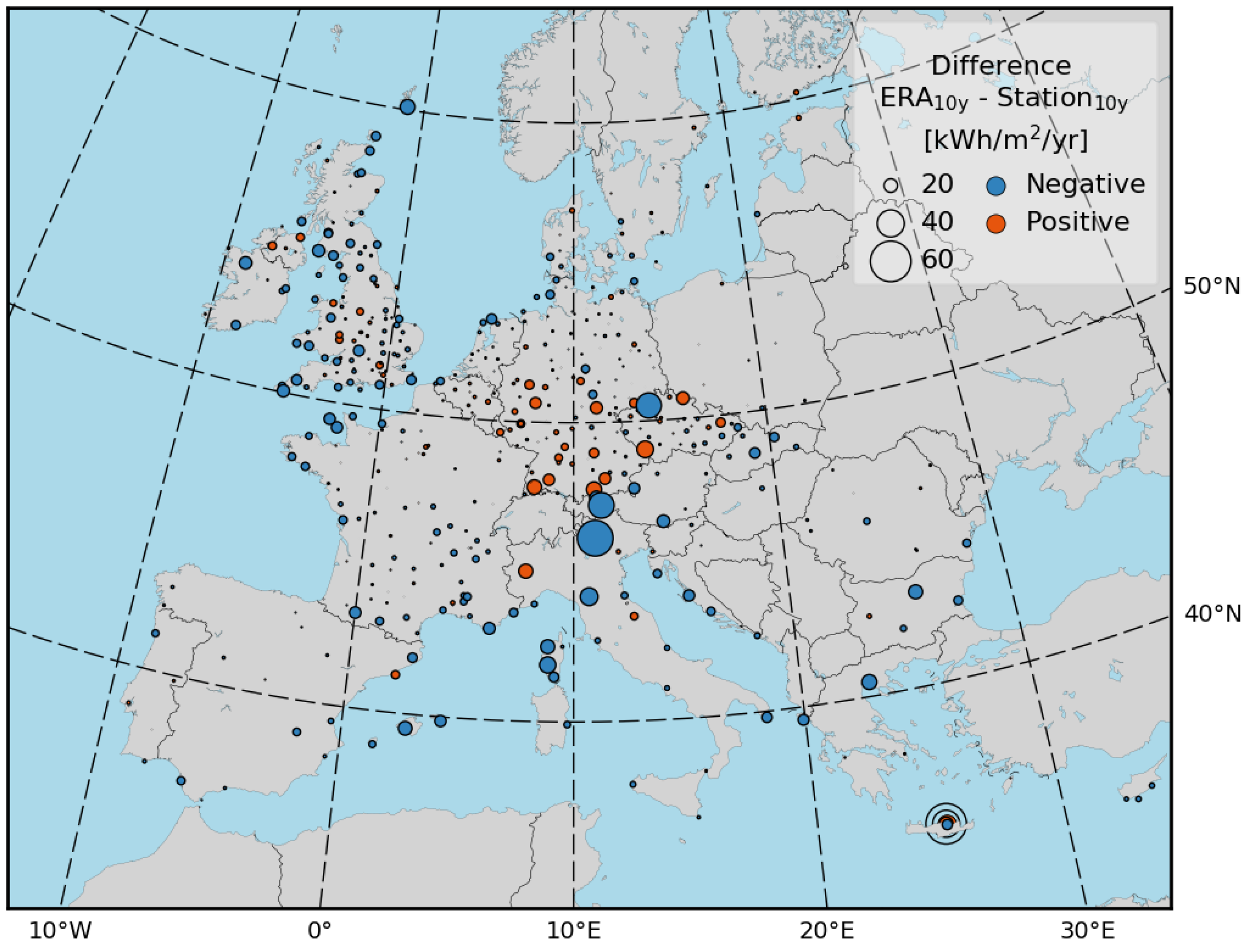
Figure 5.
Map showing difference in EnergyPlus calculation for heating energy consumption when using the station-based Typical Meteorological Year (TMY) data instead of the full 10-year station data. Values are shown as kWh/ difference, with the size of the marker indicating the magnitude of the difference. Calculation is for the single-family house configuration.
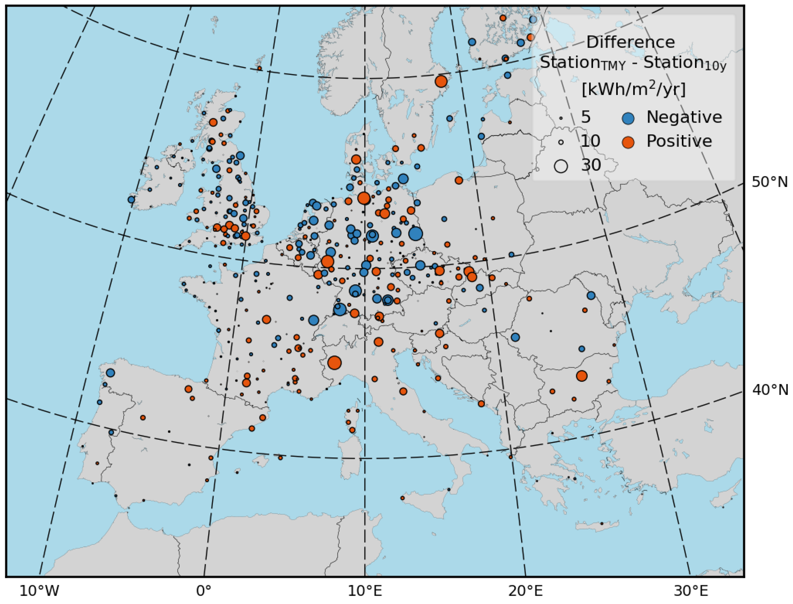
Figure 6.
Difference in EnergyPlus calculation for the single family house when using the ERA-based TMY instead of the station-based TMY data. (a) heating energy consumption; (b) cooling energy consumption. Values are shown as kWh/ difference, with the size of the marker indicating the magnitude of the difference.
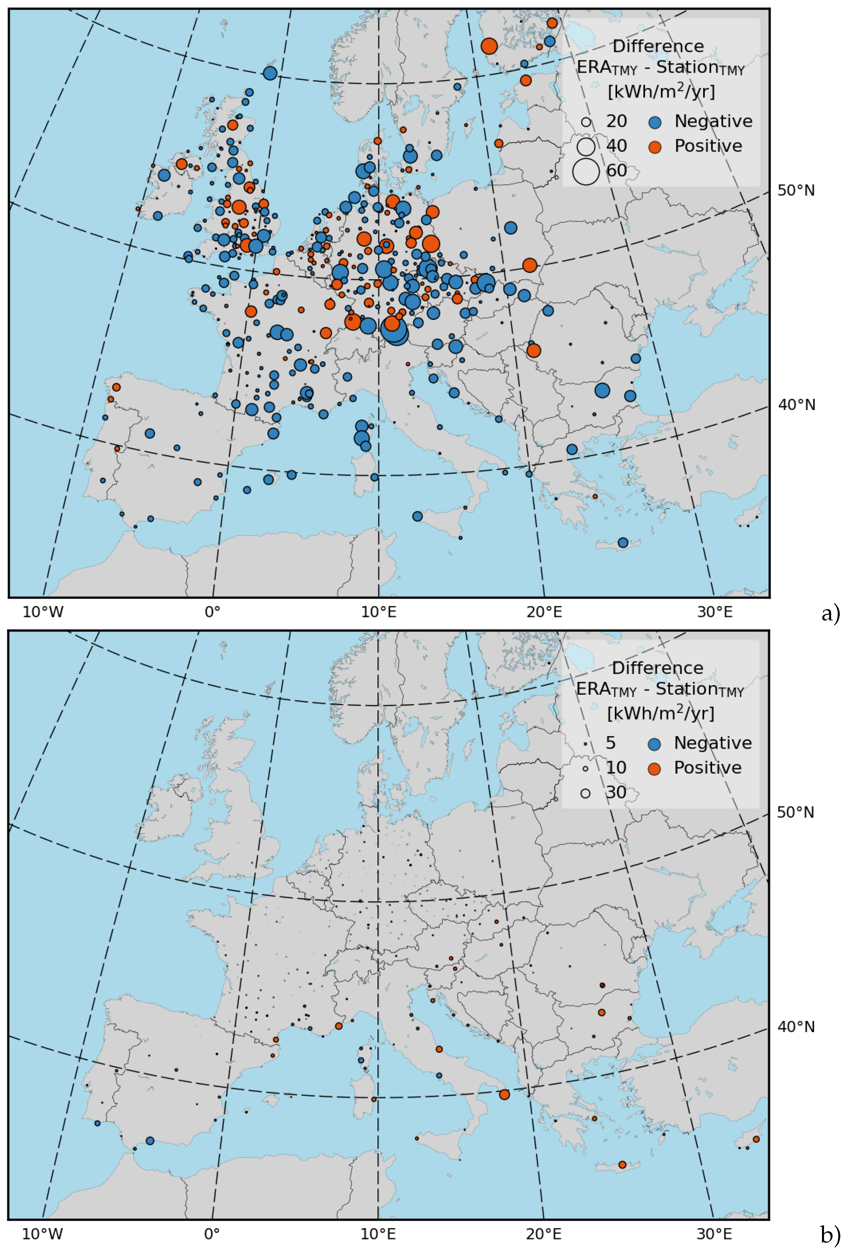
Figure 7.
Map showing relative difference (in %) in EnergyPlus calculation for heating energy calculation when using the full 10-year ERA data instead of the 10-year station data. This calculation is for the single-family house configuration.
Figure 7.
Map showing relative difference (in %) in EnergyPlus calculation for heating energy calculation when using the full 10-year ERA data instead of the 10-year station data. This calculation is for the single-family house configuration.
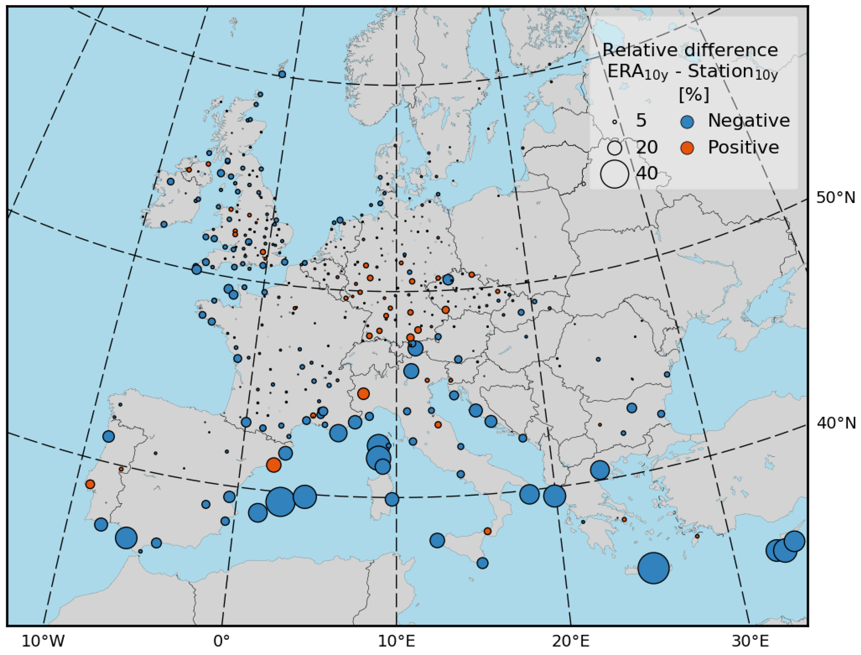
Figure 8.
Probability density functions (PDF) of air temperature for two different locations with low relative deviation in calculated heating loads (a), and high deviation (b). The PDFs are shown for the full station data, the station-based TMY, and the ERA-based TMY.
Figure 8.
Probability density functions (PDF) of air temperature for two different locations with low relative deviation in calculated heating loads (a), and high deviation (b). The PDFs are shown for the full station data, the station-based TMY, and the ERA-based TMY.
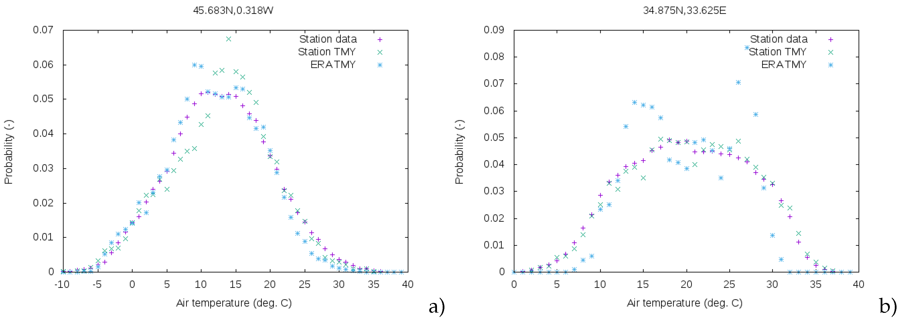
Figure 9.
Deviation in heating requirement calculation between 10-year reanalysis and station data, plotted against the Kolmogorov–Smirnov statistic for air temperature using the winter months (December–January–February) of the 10-year reanalysis and station data.
Figure 9.
Deviation in heating requirement calculation between 10-year reanalysis and station data, plotted against the Kolmogorov–Smirnov statistic for air temperature using the winter months (December–January–February) of the 10-year reanalysis and station data.
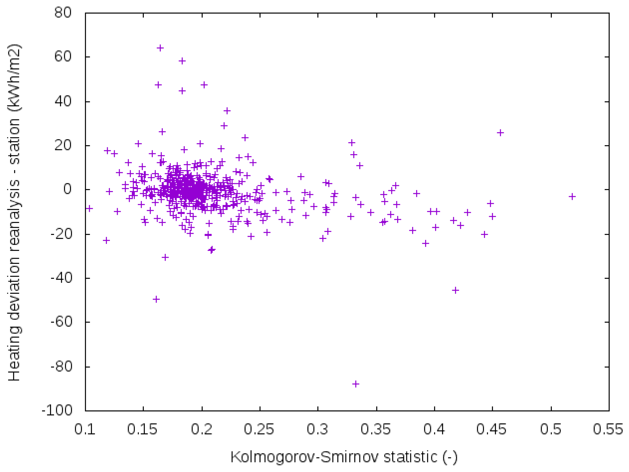
Figure 10.
Map showing difference in EnergyPlus energy consumption calculation when using the ERA-based TMY data and the station-based TMY data for an office building. (a) heating energy consumption; (b) cooling energy consumption.Values are shown in kWh/ difference, with the size of the marker indicating the magnitude of the difference.
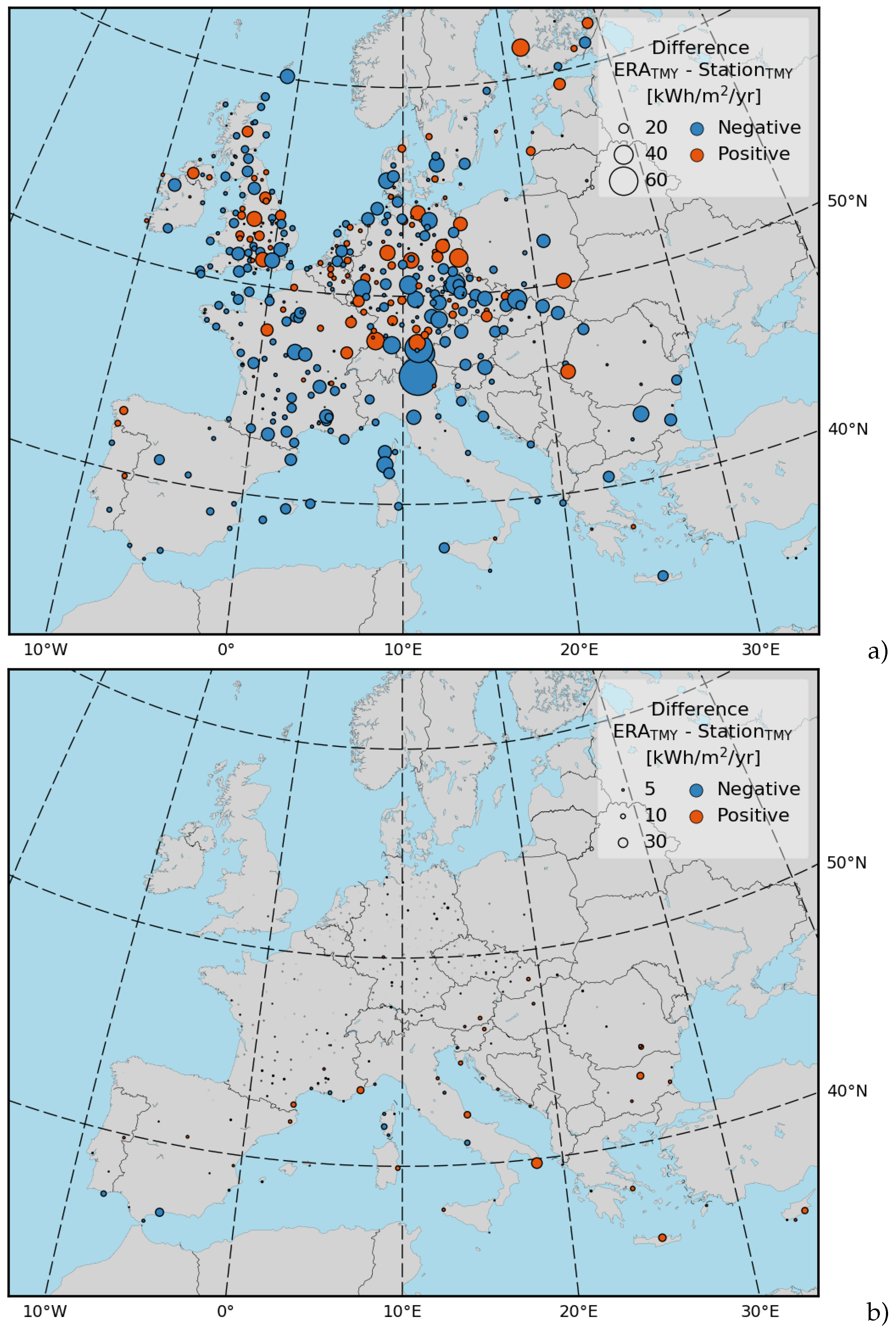
Figure 11.
Scatterplots showing heating (left) and cooling (right) requirements as calculated by EnergyPlus using either the ERA-based TMY or the station-based TMY data. Results are shown for the single-family house (top) and the office building (bottom). Note that the scale of the plots varies.
Figure 11.
Scatterplots showing heating (left) and cooling (right) requirements as calculated by EnergyPlus using either the ERA-based TMY or the station-based TMY data. Results are shown for the single-family house (top) and the office building (bottom). Note that the scale of the plots varies.

Table 1.
Parameters of the two building models used for the EnergyPlus simulations.
| Building Geometry | ||
|---|---|---|
| Parameter | House | Office |
| No. of heated floors | 2 | 5 |
| Area/Volume ratio | 0.7 | 0.33 |
| Orientation: | S/N | S/N |
| Net dimensions of heated volume (m) | ||
| Net floor area of heated zones (m) | 140 | 2400 |
| Area of S/N façade (m) | 51 | 450 |
| Area of E/W façade (m) | 51 | 240 |
| Area of Roof/basement (m) | 72.25 | 480 |
| Window area on S façade | 25% | 56% |
| Window area on E façade | 7% | 32% |
| Window area on N façade | 25% | 50% |
| Window area on W façade | 7% | 35% |
| Internal Gains | ||
| People design level (m/person) | 50 | 18 |
| Lighting design level (W/m) | 3.5 | 14 |
| Appliances design level (W/m) | 4 | 9 |
Table 2.
Average number of Heating Degree Days (HDD) and Cooling Degree Days (CDD), and statistical deviation (Mean Absolute Deviation, MAD, and Standard Deviation, SD) between different data sources calculated according to Equations (5) and (6).
| Heating | Cooling | |||
|---|---|---|---|---|
| Station Average | 2786 | 231 | ||
| Comparison | MAD | SD | MAD | SD |
| Station 10 years vs. ERA 10 years | 116.9 | 161.9 | 56.2 | 79.7 |
| Station 10 years vs. Station TMY | 132.2 | 169.0 | 41.0 | 49.3 |
| Station 10 years vs. ERA TMY | 173.8 | 221.8 | 66.7 | 89.2 |
| Station TMY vs. ERA TMY | 203.0 | 257.6 | 78.9 | 100.6 |
Table 3.
Average energy consumption and statistical deviation between different data sources calculated according to Equations (5) and (6), for the single-family house configuration.
| Heating | Cooling | |||
|---|---|---|---|---|
| Station Average () | 163.6 | 12.2 | ||
| Comparison | MAD | SD | MAD | SD |
| Station 10 years vs. ERA 10 years | 6.0 | 8.4 | 3.5 | 5.1 |
| Station 10 years vs. Station TMY | 7.6 | 9.8 | 2.0 | 2.5 |
| Station 10 years vs. ERA TMY | 10.3 | 13.0 | 3.7 | 5.1 |
| Station TMY vs. ERA TMY | 12.7 | 16.2 | 4.4 | 6.0 |
Table 4.
Average energy consumption and statistical deviation between different data sources calculated according to Equations (5) and (6) for the office building.
| Heating | Cooling | |||
|---|---|---|---|---|
| Station Average () | 80.5 | 21.6 | ||
| Comparison | MAD | SD | MAD | SD |
| Station TMY vs. ERA TMY | 9.8 | 12.8 | 6.1 | 9.7 |
Table 5.
Statistical deviation between different data sources calculated according to Equations (5) and (6) for the single-family house. All calculations are for the full 10 years of data.
| Heating | Cooling | |||
|---|---|---|---|---|
| Comparison | MAD | SD | MAD | SD |
| Station vs. interpolated station | 0.2 | 0.5 | 0.2 | 0.2 |
| Station vs. nearest neighbour | 8.2 | 11.1 | 3.6 | 5.1 |
© 2018 by the authors. Licensee MDPI, Basel, Switzerland. This article is an open access article distributed under the terms and conditions of the Creative Commons Attribution (CC BY) license (http://creativecommons.org/licenses/by/4.0/).
Share and Cite
MDPI and ACS Style
Huld, T.; Paietta, E.; Zangheri, P.; Pinedo Pascua, I. Assembling Typical Meteorological Year Data Sets for Building Energy Performance Using Reanalysis and Satellite-Based Data. Atmosphere 2018, 9, 53. https://doi.org/10.3390/atmos9020053
AMA Style
Huld T, Paietta E, Zangheri P, Pinedo Pascua I. Assembling Typical Meteorological Year Data Sets for Building Energy Performance Using Reanalysis and Satellite-Based Data. Atmosphere. 2018; 9(2):53. https://doi.org/10.3390/atmos9020053
Chicago/Turabian StyleHuld, Thomas, Elena Paietta, Paolo Zangheri, and Irene Pinedo Pascua. 2018. "Assembling Typical Meteorological Year Data Sets for Building Energy Performance Using Reanalysis and Satellite-Based Data" Atmosphere 9, no. 2: 53. https://doi.org/10.3390/atmos9020053
Note that from the first issue of 2016, this journal uses article numbers instead of page numbers. See further details here.