Effect of Wind Speed on Moderate Resolution Imaging Spectroradiometer (MODIS) Aerosol Optical Depth over the North Pacific

Abstract

The surface-wind speed influences on aerosol optical depth (AOD), derived from the Moderate Resolution Imaging Spectroradiometer (MODIS) Aqua daily observations over the central North Pacific during the period 2003–2016, have been investigated in this study. The cloud coverage is relatively low over the present investigation area compared to other marine areas, which favors AOD derived from passive remote sensing from space. In this study, we have combined MODIS AOD with 2 m wind speed (U_2m) on a satellite-pixel basis, which has been interpolated from National Centers for Environmental Prediction (NCEP) reanalysis. In addition, daily averaged AOD derived from Aerosol Robotic Network (AERONET) measurements in the free-troposphere at the Mauna Loa Observatory (3397 m above sea level), Hawaii, was subtracted from the MODIS column AOD values. The latter was to reduce the contribution of aerosols above the planetary boundary layer. This study shows relatively strong power-law relationships between MODIS mean AOD and surface-wind speed for marine background conditions in summer, fall and winter of the current period. However, previous established relationships between AOD and surface-wind speed deviate substantially. Even so, for similar marine conditions the present relationship agrees reasonable well with a power-law relationship derived for north-east Atlantic conditions. The present MODIS retrievals of AOD in the marine atmosphere agree reasonably well with ground-based remote sensing of AOD.

1. Introduction

Oceans cover approximately two-thirds of the Earth’s surface and are the major source of natural aerosol mass. In terms of mass, sea spray produced at the ocean surface dominate global aerosol flux with an annual sea salt production of 0.3 Pg to 30 Pg [1] and organic matter of 8–50 Tg C year⁻¹ [2]. Due to high hygroscopicity of sea salt and regional abundance, the aerosol provides a major contribution to the scattering of solar radiation, resulting in a cooling effect [3,4,5,6,7]. Moreover, serving as an efficient cloud condensation nuclei the sea salt aerosol exerts a strong influence on cloud formation, properties and lifetime [8,9]. The importance of sea-spray aerosol’s impact on the radiative balance, both on global and regional scales, has led to extensive research. This has aimed for a better understanding of emissions, composition, transformation, transport and removal, as well as interactions with radiation and clouds, (e.g., [1,10,11,12,13,14]). To represent oceanic aerosols explicitly in global climate models it is necessary to describe primary marine aerosol emission fluxes quantitatively, with respect to their size and chemical composition [13].

The main physical parameters that determine sea-spray aerosol production are: (i) sea ice cover ([10]; (ii) wind speed [10,15]; and (iii) surface water temperature [11,16,17]. Sea ice acts as a lid over the sea and over open leads between ice floes, and the ice limits the fetch and prevents wave breaking, which is needed for sea-spray formation. At an ice cover of about 80–90% the sea-spray emissions are reduced with one order of magnitude over the patches of open water, and on average by two orders of magnitude over larger areas of the same ice fraction, compared to open sea. The wind stresses the ocean surface and when waves break air is entraining into the water. Air bubbles rise to the surface, creating white colored areas (whitecaps), where they eventually burst and release aerosol droplets into the atmosphere [1,18,19,20]. The wind effect on sea spray production is often included in the source parameterizations through an expression of the white cap coverage, but it can also be done through the amount of entrained air [17]. The effect of increasing wind is highly non-linear and results in about a factor 10 increase in sea-spray emission per 10 m/s increase. The water temperature changes the bubble spectra through the combined influence of surface tension, viscosity, coalescence, rise velocity and oxygen saturation [11,16]. The net effect is a decreasing sea-spray production with an increasing water temperature. Although there have been many achievements in understanding sea-spray aerosol production, the uncertainty in existing parametrizations remains sufficiently large [1,13]. Recently proposed parametrizations of the production flux result in two orders of magnitude higher aerosol concentrations simulated than observed, raising questions about the validity of such estimates and methods to attain them [13].

Unlike the continental atmospheric boundary layer, the marine atmospheric boundary layer has mostly a near-neutral stratification and, thus, we do not expect to find a well-mixed layer. In addition, decoupled layers frequently occur over the ocean [21,22,23,24,25] that create vertical gradients in sea-salt aerosol concentrations in the lower troposphere [12,14,26,27,28,29,30]. Relatively strong vertical gradients have also been observed and modeled for coarse mode aerosols (>0.5 μm radius), and modeled for submicron aerosols, in otherwise well-mixed marine boundary layers (MBLs) without thermodynamic evidence of decoupling [12]. These findings are explained by the gravitational deposition velocity of the coarse-mode particles. This implies that in situ measurements of sea-salt concentration at one altitude do not represent the entire marine boundary layer.

Since winds near the surface are an important factor in the formation of breaking waves and bubbles that burst [10,13,31], which results in the release of sea-spray aerosol, this supports investigations of the relationship between aerosol optical depth (AOD) and surface-wind speed. The other two major physical drivers, sea ice and surface-water temperature, change much slower than the wind speed, for which the variation is found on a time scale smaller than about five days (the synoptic time scale). It is therefore possible to study the effect of surface-wind speed on AOD separated from temperature and sea ice even at high latitudes. The wind dependency allows for the establishment of an empirical relationship between AOD and wind speed that can be used in global and regional model simulations and/or, more importantly, for evaluating model simulations of AOD in the marine atmosphere.

The AOD–wind speed relationship has been investigated in several previous studies, although there is no consensus between the findings. Some studies suggest a linear relationship [32,33,34,35], while others a power-law relationship [14,36,37] or an exponential relationship [38]. The discrepancy between different relationships is probably attributed to different instrumentations, platforms, locations and periods used in the investigations.

In the present study, we investigate how wind speed influences AOD that is derived from the Moderate Resolution Imaging Spectroradiometer (MODIS) daily observations over the North Pacific during the period 2003–2016. The relationship estimated between AOD and surface-wind speed is compared to results obtained in several previous studies. In addition, we examine how surface-wind speed influences the contribution of coarse and fine-mode aerosols to the AOD. The satellite-derived AOD is validated against sun photometer measurements carried out at stationary ground-based sites and during ship cruises.

2. Data, Methodology and Investigation Area

2.1. Moderate Resolution Imaging Spectroradiometer (MODIS) Aerosol Retrievals

MODIS on the Aqua satellite measures scattered sunlight at 36 spectral frequencies and provides daily global aerosol products. From 700 km above sea level and with nadir views, between the latitudes 0° and 55°, MODIS observes the planet with a swath of about 2330 km. MODIS Aqua makes 14–15 orbits per day with local equatorial crossing time approximately 13:30 (ascending node). All MODIS data are organized into 5-min intervals or granules. With a 10 × 10 km spatial resolution at nadir, the output grid results in 135 × 203 pixels for one granule.

MODIS retrievals of AOD over the land and ocean are based on the dark-target algorithm, thoroughly described in the literature [39,40,41,42,43,44]. The algorithm calculates AOD over an expected dark surface, while over the ocean the effects of sun glint and the presence of foam (whitecaps) on the water need to be accounted for. The retrievals of AOD, both over land and ocean, are based on look-up tables (LUTs), where normalized satellite-detected scattered radiance are compared with pre-computed radiative transfer, with a set of likely aerosol situations as well as prescribed Rayleigh scattering and surface reflection. The ocean algorithm consists of nine tropospheric aerosol model types: four fine modes (with effective radius (r_e) < 0.25 μm) and five coarse modes (r_e > 1.0 μm), where each type is a single mode of log-normal size distribution. To relate the measured reflectance to AOD, the algorithm finds a solution of weighted combinations of fine and coarse modes that approximates best the observed spectral reflectance [43]. MODIS data is presented in different collections consisting of data products that were generated by similar but not necessarily the same versions of the retrieval algorithm. The AOD that is derived by the MODIS land and ocean retrievals at 555 nm has expected error envelopes of ΔAOD = ±0.05 ± 0.15·AOD [42] and ΔAOD(+) = +0.04 + 0.1·AOD/ΔAOD(−) = −0.02 − 0.1·AOD [43], respectively.

In this study, we use MODIS Aqua Collection 6 (C6) level 2 standard 10-km products for best-quality retrievals (quality flag = 3) of AOD, mainly over the ocean surface. Data were taken from the National Aeronautics and Space Administration (NASA) Goddard Space Flight Center’s Atmosphere Archive and Distribution System (http://ladsweb.nascom.nasa.gov). In previous MODIS collections, the calculation of sun glint and foam on the water surface were based on a single value of wind speed (6 m/s) and foam fraction (0.16%) [43]. For better representation of the surface roughness, additional wind speeds (2 m/s, 10 m/s and 14 m/s) and corresponding foam fractions (0.01%, 1% and 3%) were added to MODIS C6. C6 also includes 2 m wind speed (U_2m) on a satellite-pixel basis, which has been interpolated from National Centers for Environmental Prediction (NCEP) reanalysis (1° × 1°) GDAS 10 m wind data as a required ancillary field. In addition to total AOD and U_2m, aerosol size parameters such as Ångström exponent and contribution of fine-mode aerosols to the AOD, have also been investigated. The MODIS Ångström exponent (α_MOD) has been calculated based on AOD retrieved at the two wavelengths 555 nm and 858 nm:

$${\mathsf{\alpha }}_{\mathrm{MOD}}=-\frac{\ln \frac{{\mathrm{AOD}}_{{\mathsf{\lambda }}_{555}}}{{\mathrm{AOD}}_{{\mathsf{\lambda }}_{858}}}}{\ln \frac{{\mathsf{\lambda }}_{555}}{{\mathsf{\lambda }}_{858}}}$$

(1)

2.2. Aerosol Optical Depth (AOD) from Sun Photometer Measurements

The Aerosol Robotic Network (AERONET) provides ground-based measurements of aerosol optical properties. AERONET is equipped with Cimel sun photometers that measure direct sun radiance at eight spectral bands. Measurements are taken every 15 min during daylight hours and are available in three categories: level 1.0 (unscreened), level 1.5 (cloud screened) and level 2.0 (quality assured). In this study, level 2.0 data are used. AERONET-derived AOD are expected to be accurate within <±0.01 for wavelengths longer than 440 nm, (e.g., [45]). The component of AERONET, Maritime Aerosol Network (MAN), provides ship-borne AOD measurements with Microtops II sun photometers calibrated at the NASA Goddard Space Flight Center. The estimated uncertainty of the MAN AOD does not exceed ±0.02 [46].

To validate MODIS AOD we compared the retrievals against AOD derived from AERONET observations at the three ground-based stations: Lanai (20 m, 20.7° N, 156.9° W), Coconut Island (0 m, 21.4° N, 157.8° W) and Midway Island (0 m, 28.2° N, 177.4° W). Observations during several cruises predominant in the North Pacific (

Table 1. List of Maritime Aerosol Network (MAN) cruises, investigation areas, and number of measurement days.

Year	Cruise Name	Investigation Area	Time Period	Duration
2016	NOAA Ron Brown	North Pacific Ocean	May	8 days
2015	Okeanos Explorer	Around Hawaiian Islands	September	7 days
2013	Horizon Spirit	North Pacific Ocean	June–August	21 days
2013	RV Kilo Moana	Around Hawaiian Islands	August–September	13 days
2012	RV Sonne	Pacific transect from Japan to Fiji Island	September–October	14 days
2012	RV Trans Future 5	Pacific transect from New Zealand to Japan	June	6 days
2012	Horizon Spirit	Eastern North Pacific Ocean	September and October	9 days
2012	RV Thomas G. Thompson	West coast of Mexico, North Pacific	March–April	14 days
2011	RV Kilo Moana	Around Hawaiian Islands	February	8 days
2010	RV Roger Revelle	Philippine Sea, North Pacific Ocean	September–October	11 days
2010	MV Zim Iberia	Gulf of Mexico, Pacific Ocean	March–May	41 days
2009–2010	RV Melville	Pacific latitudinal transect from Brisbane, Australia across the Southern Pacific to South America	November–February	42 days
2009	RV Sonne	Western Pacific Ocean	October	7 days
2008	MS Trans Future 5	Pacific transect from New Zealand to Japan	August–September	13 days
2007	MS Trans Future 5	Pacific transect from New Zealand to Japan	May–June	7 days

) have also been used in the validation. AOD from AERONET and MAN is available at the 500 nm wavelength. We adjusted the AERONET and MAN AOD values to correspond to the MODIS AOD wavelength of 555 nm using the Ångström power law:

AOD₅₅₅ = AOD₅₀₀ × exp[−α_AER ln(555/500)]

(2)

where α_AER is the AERONET Ångström exponent derived from the wavelengths 440 nm and 675 nm.

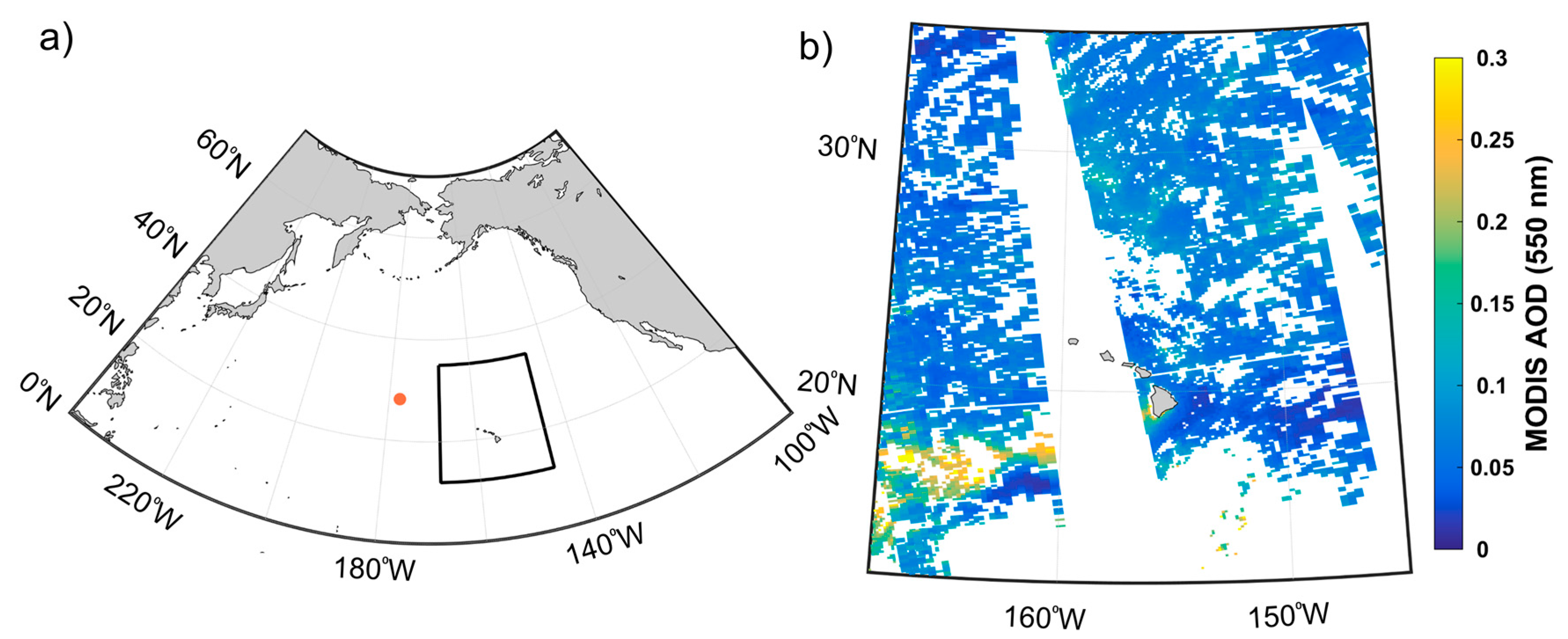
2.3. Investigation Area: Central North Pacific

Figure 1 shows the investigation area (12.0° N to 35.0° N, 145.0° W to 168.0° W) in the central North Pacific and an example of a MODIS Aqua scene with AODs for 18 September 2014. All MODIS Aqua AODs that are available within the black box and corresponding to the period 2003–2016 are included in the investigation. This results in 26,210 granules of C6 data. This area was chosen in order to minimize the influence from continental aerosols on the air masses investigated, This region is highly influenced by a persistent sub-tropical high-pressure system, which shifts north during the summer months and south during the winter season. The cloud coverage is relatively low over the central North Pacific compared to other marine areas, which favors satellite retrievals of AOD. The north-eastern trade-winds over this region are very consistent. They prevail around Hawaii between 85% and 95% of the time during summer and around 50% to 80% of the time during the winter season [47].

2.4. FLEXible TRAjectories (FLEXTRA) Trajectory Model

FLEXible TRAjectories (FLEXTRA) were used to calculate mean wind trajectories operating directly on data from the European Centre for Medium-Range Weather Forecasts (ECMWF). Meteorological-level fields from the ECMWF T213 L31 model were used. FLEXTRA has an ensemble option to assess the accuracy of the trajectories, and different options for the interpolation of the wind data. For more details of the FLEXTRA model, see [48,49]. In this study, we analyzed trajectories that run 7 days back in time from Mauna Loa mountain station (19.54° N, 155.58° W, 3000 m above sea level, Figure 1), Hawaii, with starting times 00, 06, 12 and 18 UTC each day within the period 2003–2010.

3. Results

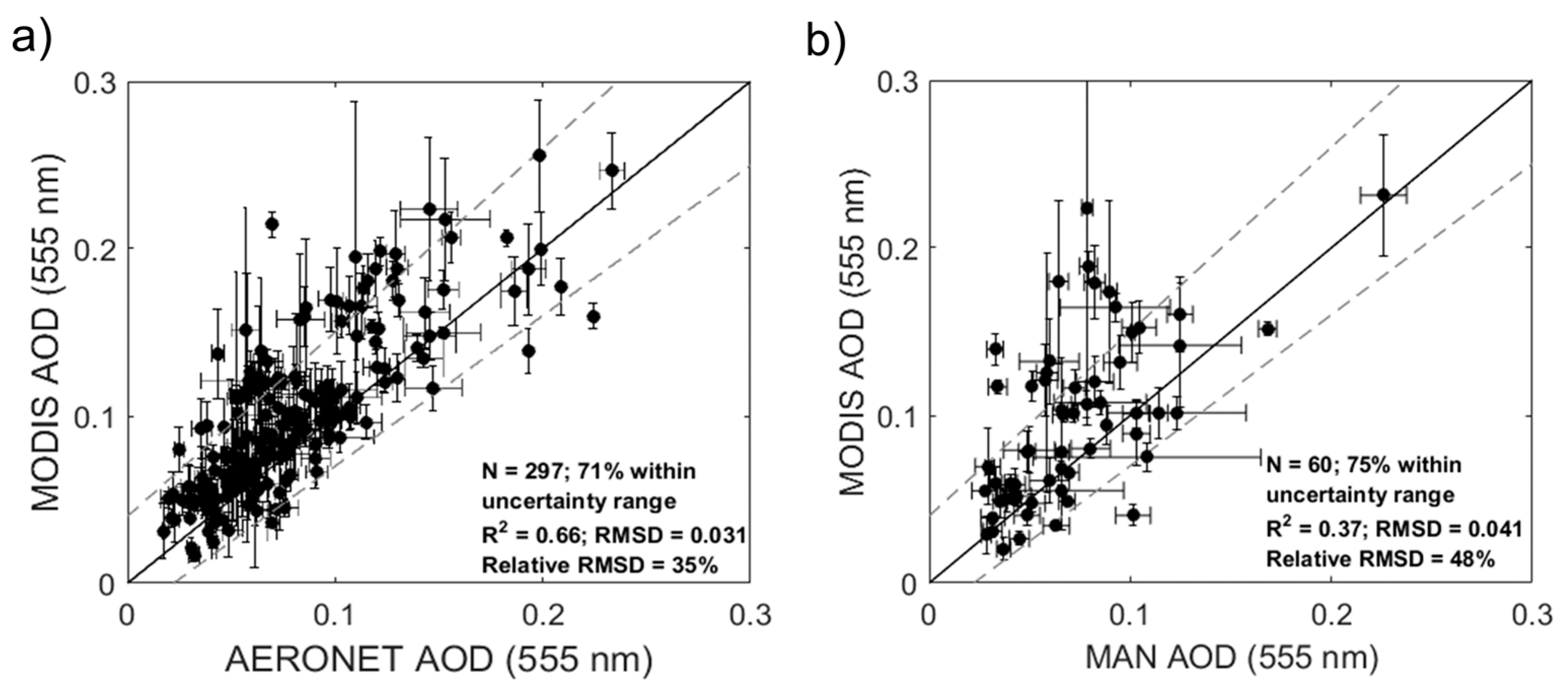
3.1. Validation of MODIS AOD against Ground-Based Measurements

Figure 2a,b shows comparisons of MODIS AOD against AOD derived from AERONET and MAN measurements, respectively, carried out at coastal ground-based stations and during ship cruises, respectively. We used a box of 3 × 3 pixels (30 × 30 km) around each ground-based station or ship, although only cases with an availability of at least three AOD values were included in the comparison. In addition, satellite overpass windows of 30 min and 2.5 h were used here for AERONET and MAN, respectively. Previous studies have shown that MODIS retrievals of AOD over coastal sites are associated with significant uncertainties (Section 4), although when using the 30-min time window reasonable agreement between MODIS and AERONET was obtained (see below). The relative (normalized) root mean square deviation (relative RMSD) was determined for collocated satellite and ground-based AOD values, averaged according to the procedure described in [50].

Figure 2a shows that MODIS AOD agree reasonably well with sun photometer measurements carried out at the three marine ground-based sites. Most AOD values are below 0.2. In the validation against AERONET, the percentage of the MODIS values that is within the expected uncertainty is 71%. For ship-born measurements, 75% of the collocated points lie within the expected uncertainty (right figure). The vertical and horizontal error bars in Figure 2 show that some of the MODIS and AERONET/MAN AODs are associated with large variability.

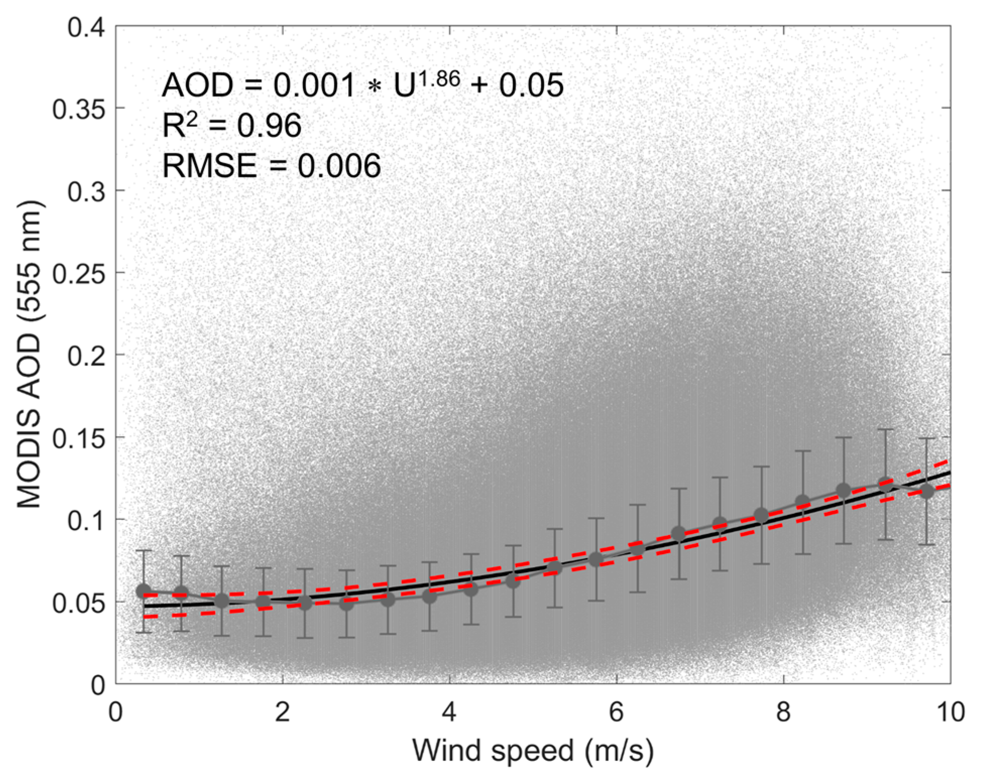
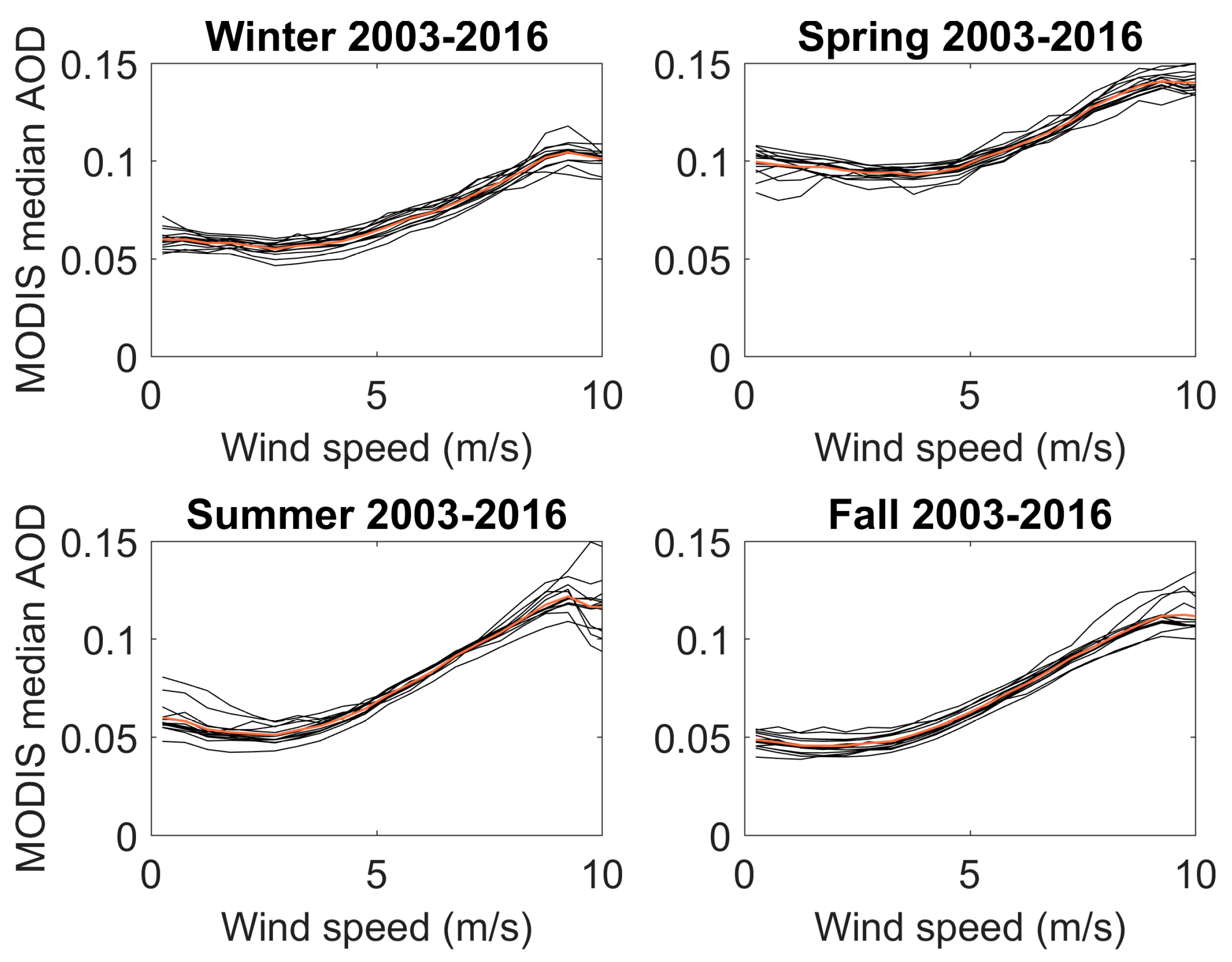
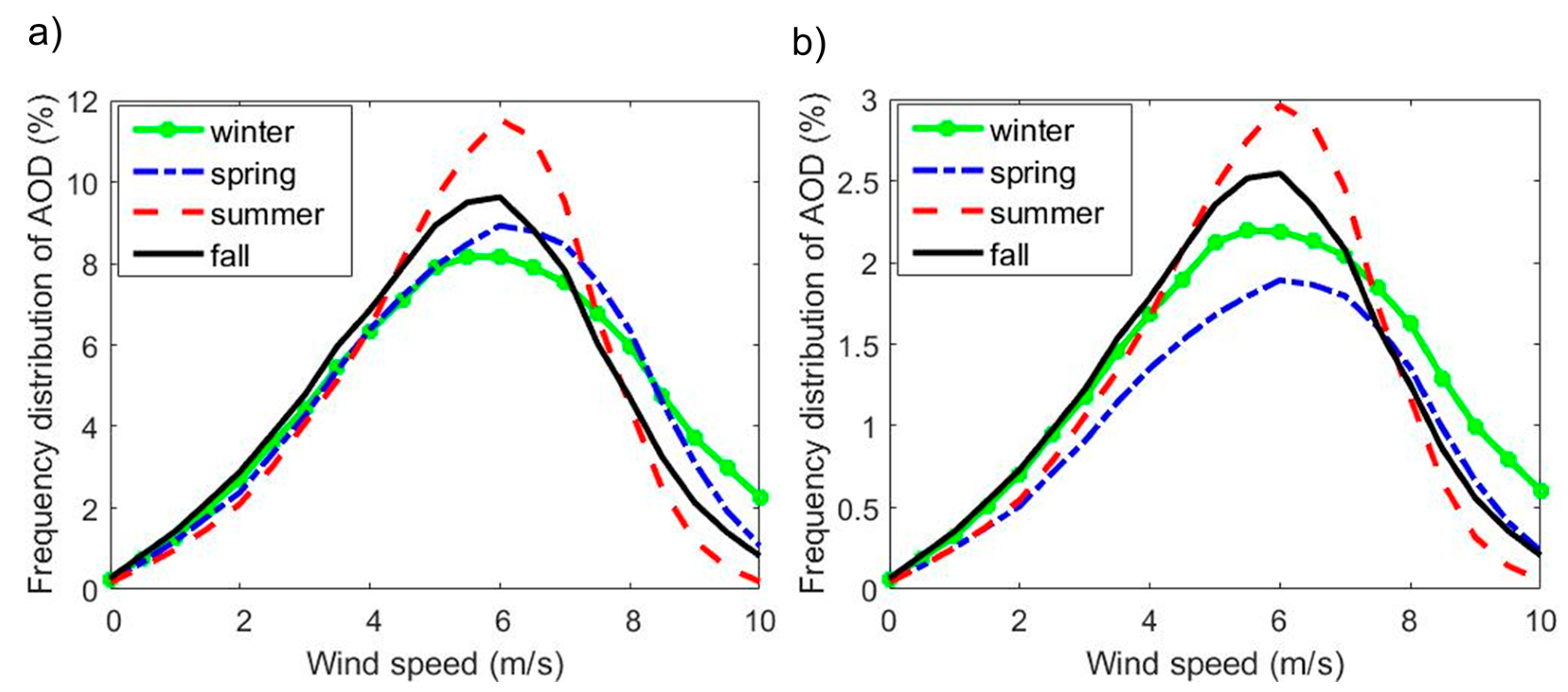
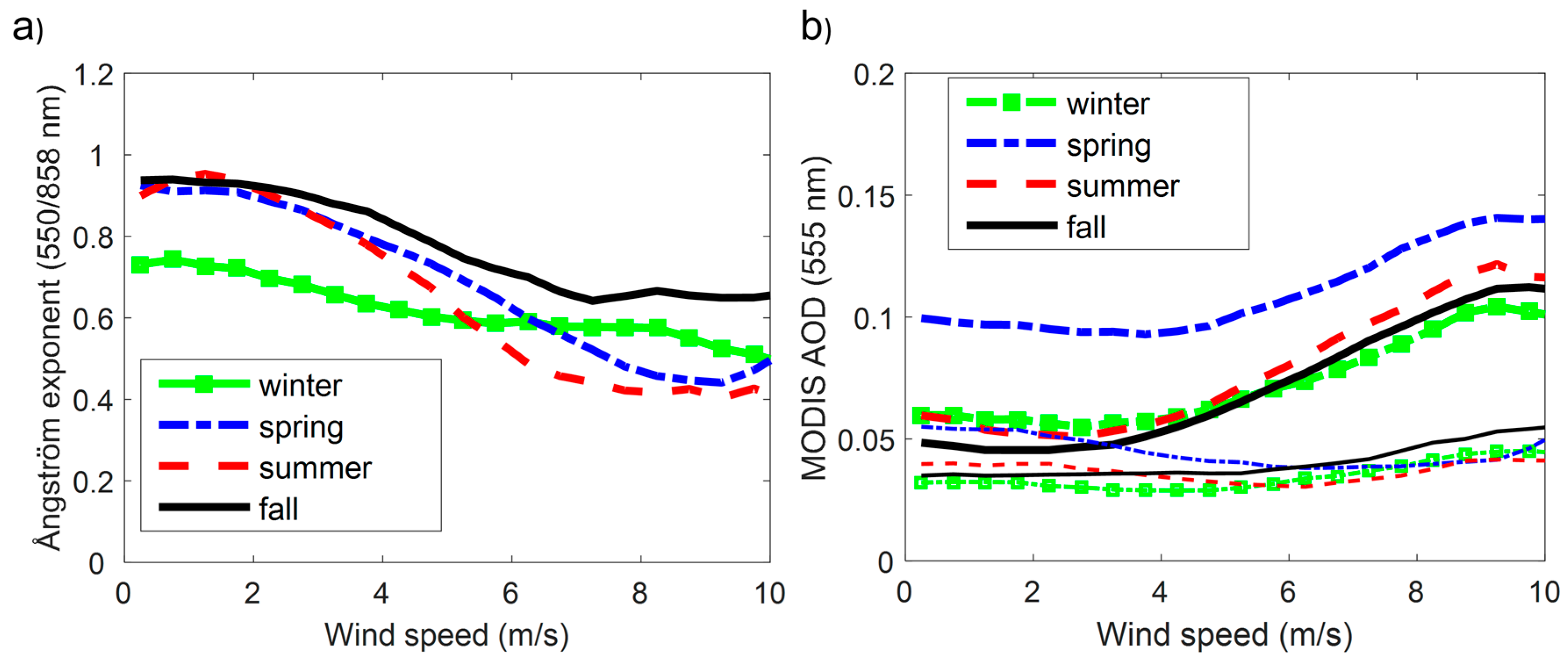
3.2. Evaluation of MODIS-Derived AOD versus Surface Wind Speed

Fourteen years (2003–2016) of MODIS daily column AOD, at the wavelength 555 nm, have been matched with surface (2-m) wind speed over the central North Pacific. However, daily averaged AERONET AOD measured in the free-troposphere at the Mauna Loa Observatory (3397 m above sea level, 19.54° N, 155.58° W), Hawaii, was subtracted from the MODIS column AOD values. The latter was undertaken to reduce the contribution of aerosols above the planetary boundary layer, which are expected to be weak related to surface-wind speed. For the few days with missing AERONET data we used AOD averaged over the two neighboring days. The adjusted AOD values were binned with respect to surface wind speed, with bins of 0.5 m/s within the range 0–10 m/s.

Figure 3 shows an example of all MODIS-adjusted AOD values on a pixel basis, versus surface-wind speed, derived from observations over the present investigation area during summer 2007. Cases with AOD values around and below 0.1 suggest that natural background aerosol was dominating, while the higher values may be due to hazier conditions and/or the effects of cloud contamination. However, the median absolute deviation suggests that the latter values are relatively few with respect to all AODs. Figure 3 shows that the median AOD starts to rise at a wind speed about 3.5 m s⁻¹, although a decrease appears for the highest wind speeds.

Furthermore, Figure 4 presents only the binned data on a seasonal basis, although for all years investigated here. The winter, spring, summer and fall seasons are represented by the months December–February, March–May, June–August and September–November, respectively. In summer, fall and winter Figure 4 shows that the median AOD increases roughly by a factor of 2 within the wind speed range about 3.5–9 m/s. In spring the increase in AOD is similar in absolute terms, however, the background AOD is substantially higher than in other seasons. This is likely due to the influence of continental aerosols (Section 4). Moreover, as in Figure 3, MODIS AOD do not exhibit an increase at wind speeds higher than ~9 m/s for any of the seasons (further discussed in Section 3.7).

Figure 4 shows that the MODIS-adjusted median AOD for the lower wind speeds in spring is about two times higher than in other seasons, and about 25% higher for the highest wind speeds. The figure also shows that the mean AODs (orange solid line) estimated for low wind speeds for winter are somewhat higher than AODs corresponding to summer and fall (more clearly shown in Figure 6b. The rate of change in AOD with increasing wind speed is smaller for winter than the other seasons.

Figure 5a,b show seasonal wind speed probability density function for MODIS derived AOD, normalized according to the total number of derived AOD corresponding to a season and year, respectively. The majority of the AOD values were derived at wind speeds in the range between about 3.5 m/s and 8 m/s; thus, rather few AOD values correspond to lower and higher wind speeds.

For the most common wind speeds, Figure 5b shows that summer is associated with the highest number of available AODs. However, with the exception of 2011, 2014, 2015 and 2016 the winter season is associated with the highest number of available AODs over the entire wind speed range (not shown). In addition, more available AODs at the highest wind speeds in winter may be attributable to a higher frequency of low pressures in the westerly flow over the North Pacific (Section 3.4). The minimum number of observations is found for spring, with the exception of 2014 (not shown).

To identify whether the change in adjusted AOD with increased surface-wind speed is caused by sea-spray aerosol, within a particular size-range, we investigated the MODIS-derived Ångström exponent and the contribution of fine mode aerosols to the AOD. Figure 6a shows the seasonally averaged Ångström exponent according to the period 2003–2016 versus surface-wind speed. Since the extinction efficiency of larger-sized aerosol particles is nearly spectrally neutral, the decrease in the Ångström exponent indicates a shift towards larger aerosol particles at higher wind speeds. At lower wind speeds, the production of sea spray is low and it is reasonable to assume that the presence of secondary sub-micron aerosols such as ammonium sulfate, and maybe also organic compounds, dominates over the central North Pacific. The decrease in the Ångström exponent is evident for the current wind-speed range, although for winter the decrease is less salient compared to the other seasons.

Figure 6b shows the contribution of MODIS fine-mode adjusted AOD (for aerosols smaller than 0.5 μm in diameter) to the total adjusted AOD at 555 nm plotted against surface-wind speed and averaged over the period 2003–2016. Here, we focus on the results obtained for summer, fall and winter, for which we expect influences mainly from marine background aerosols. As shown in Figure 6b, the relationship between AOD and wind speed consists of two visible phases: AOD associated mainly with fine-mode aerosols at lower wind speeds and a distinct increase of larger aerosols that starts to occur around 3.5 m/s. Note, it is suggested that that white caps start to form at wind speeds of around 3.5 m s⁻¹ [51,52,53,54]. Even so, the parameterizations derived in the first three studies for low wind speeds, 3–5 m s⁻¹, include whitecap fractions that differ by more than one order in magnitude [53]. Figure 6 shows that the lowest contribution of fine-mode aerosols to the total AOD at low wind speeds is occurring in winter, which is in line with the results of the Ångström exponent. This finding could be consistent with a contribution from secondary aerosol formation to fine aerosol, which should be smaller in winter due to a lower biological production.

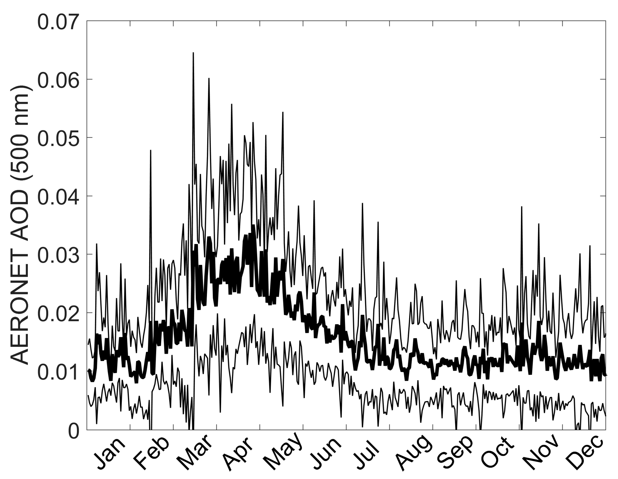
3.3. Aerosol Robotic Network (AERONET) Free Tropospheric AOD

Aerosols in the entire atmospheric column, between the sea surface and the top of the atmosphere, contribute to the AOD derived from MODIS observations. Quantifying the relative contributions of the boundary-layer and free-tropospheric aerosols to the total column AOD is not possible with passive remote sensing from the space and ground. Without deep convection that can effectively transport aerosols from the boundary layer to higher elevations in the free troposphere, long-range transport is expected to have a greater role in determining the number of aerosols in the free troposphere. The AERONET observation site at mount Mauna Loa is mostly above the boundary layer and, therefore, occasionally affected by long-range transport of anthropogenic aerosols.

Figure 7 shows the annual cycle of AOD that was measured at the Mauna Loa site during the period 2003–2016. The most evident feature is the springtime AOD, which is about 2–3 times higher than in the rest of the year. Furthermore, the figure indicates that the averaged AOD derived from observations at Mauna Loa make up about 20% of the total column AOD (Figure 6b) for the central North Pacific in summer, fall and winter.

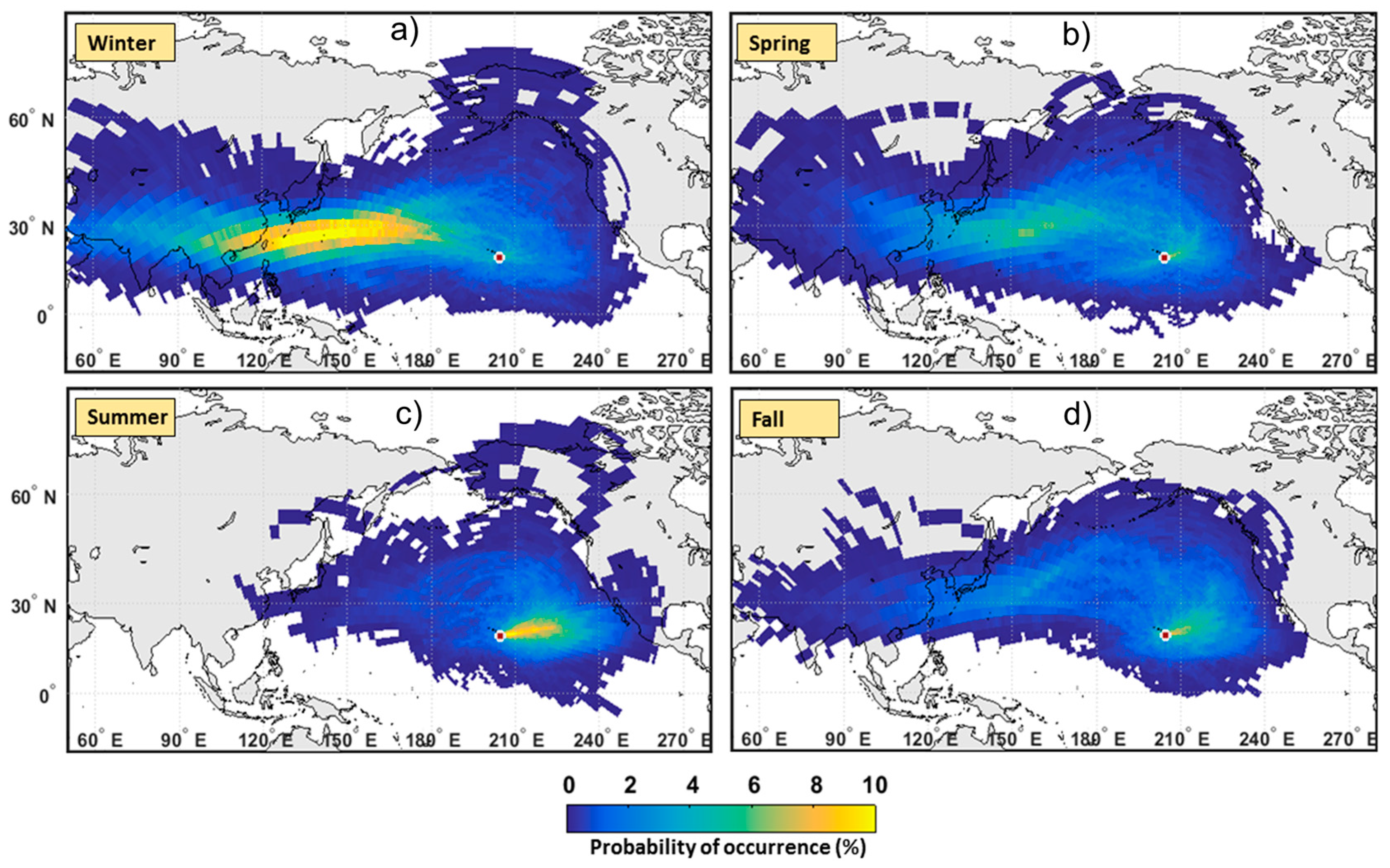
3.4. Air Mass Transport

Analyzing a large number of back-trajectories helps in evaluating influences of long-range transport of aerosols on the observed annual cycle of the MODIS and AERONET AOD. In Section 3.2 and Section 3.3 it was demonstrated that AOD peaks in spring—in the free troposphere as well as in the boundary-layer during both low and high wind speeds. Figure 8 displays seasonal density of the FLEXTRA 7-day back-trajectories for the period 2003–2016. The trajectory density reflects the probability of a trajectory crossing any grid cell (regardless of the trajectory altitude) and highlights the source regions of the air masses in each season. The figure suggests that air masses approach Mauna Loa from the north-eastern sector mainly in summer. It also shows that the area covered by the 7-day trajectories is larger and extends further to the west in winter and spring. Thus, it is more likely that the air masses in these seasons to a larger extent arrived from southern and central Asia before reaching the Hawaii region.

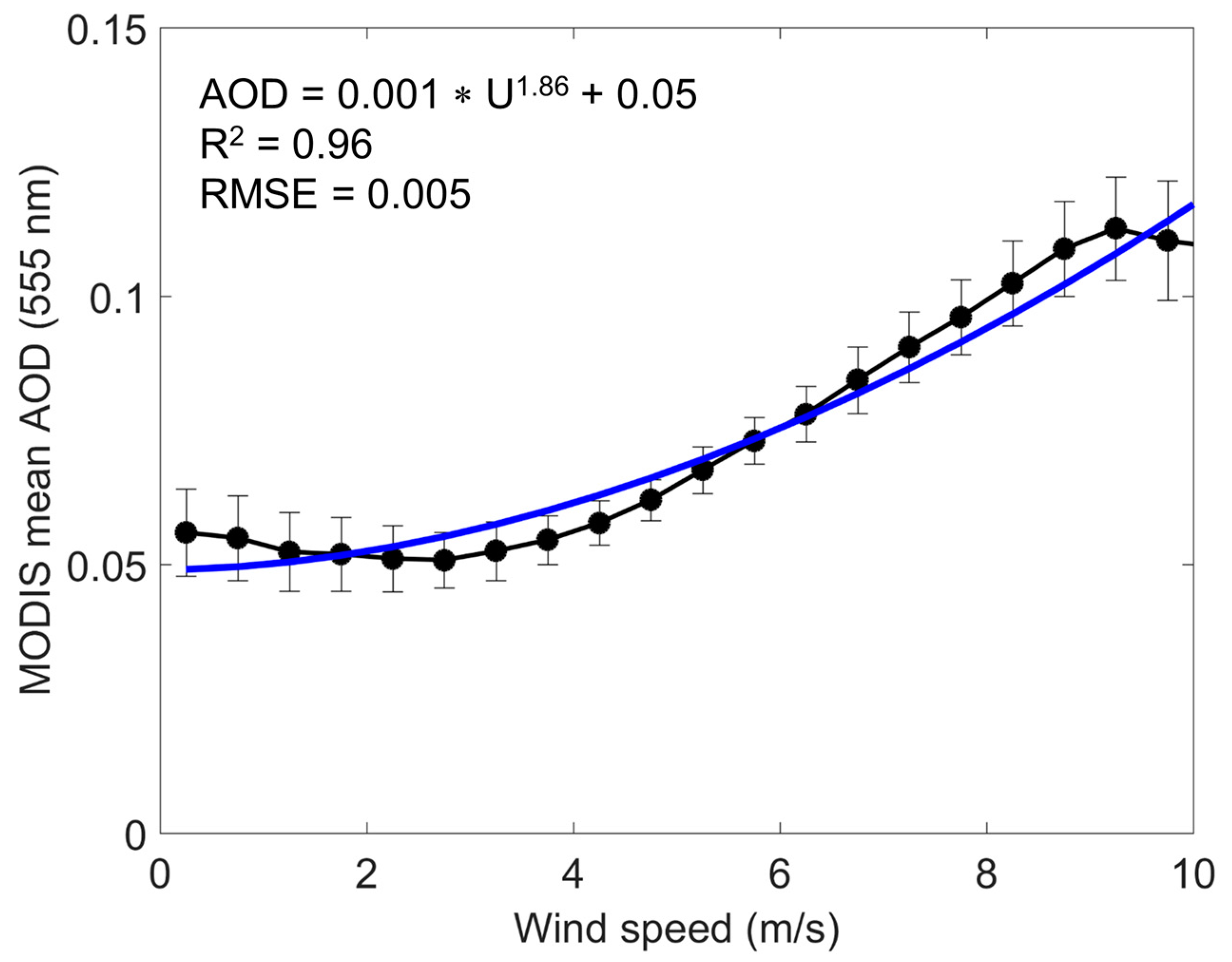
3.5. Power-Law Relationship between MODIS AOD and Surface-Wind Speed

The relationship between AOD and surface-wind speed is often represented by a power-law function. Figure 9 shows annual mean MODIS-adjusted AOD (black circles) and corresponding one standard deviation for the period 2003–2016, although excluding the spring season due to substantially higher AOD values compared to the other seasons. The derived power law relationship, AOD = 0.001 × U^1.86 + 0.05, indicate a relatively strong wind dependency. The constant zero offset term (AOD ~ 0.05) reflects a marine background situation, where we assume the presence mainly of secondary aerosols such as ammonium sulfate that are formed independently of the local wind speed. However, the relatively long turn-over time for the submicron sea-salt particles (27) means that they may contribute to AOD also during situations with low wind speeds. Even so, we believe a minor contribution from these aerosols, since the local wind speed is probably a good substitute for the Lagrangian wind speed over the accumulation-mode lifetime (10).

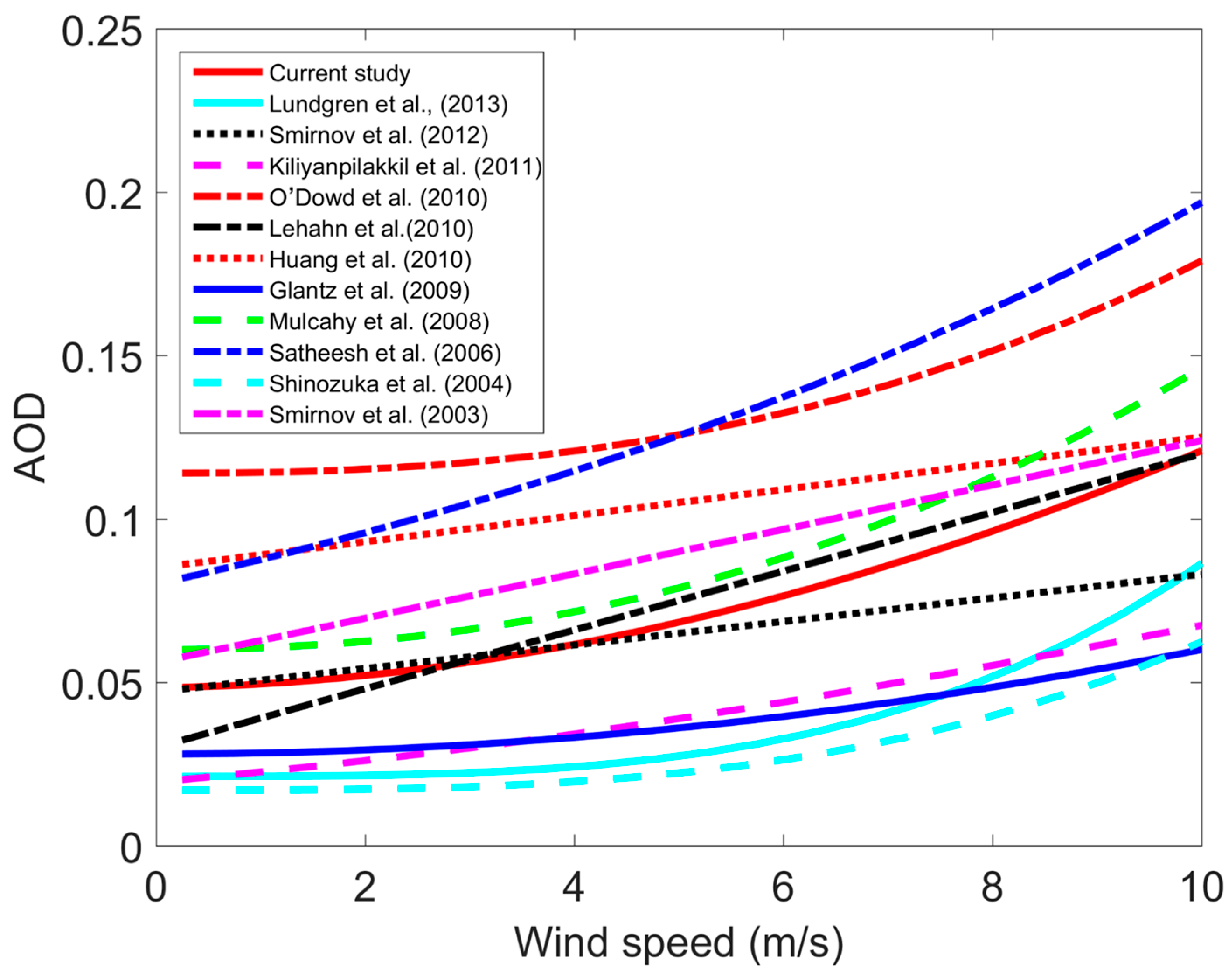
3.6. Comparison with Previous Studies

Figure 10 and

Table 2. Current and previous parametrizations of AOD as a function of surface wind speed.

Relationship	Type	R2	Investigation Period	Region	References
AOD555 = 0.001 × U1.86 + 0.05	power-law	0.95	2003–2016 (fall, winter, summer)	NP a	Current study (MBL h AOD)
AOD555 = 0.001 × U1.83 + 0.06	power-law	0.96	2003–2016 (fall, winter, summer)	NP	Current study (Column AOD)
AOD550 = 2.594 × 10−5 × U3.3992 + 0.0212	power-law	n/a	n/a	S b	[14]
AOD550 = 0.00022 × U2.47 + 0.114	power-law	0.89	December 2006	NP	[56]
AOD555 = 0.00032 × U2.3 + 0.028	power-law	0.98	September 2001	NP	[37]
AOD500 = 0.00055 × U2.195 + 0.06	power-law	0.97	January 2002–December 2004 (total 14 days)	MH c, NA d	[36]
AOD500 = 0.0036 × U + 0.047	linear	0.33	Different times	Global	[55]
AOD532 = 0.15/(1 + 6.7e−0.17×U)	logistic	0.97	June 2006–April 2011	Global	[35]
AOD500 = 0.009 × (U − 4) + 0.03	linear	0.45	2002–2008	Global	[33]
AOD550 = 0.004 × U + 0.085	linear	0.95	2004	Global	[34]
AOD500 = 0.0068 × U + 0.056;	linear	0.14	January 2001–February 2002	MI e, NP	[32]
AOD550 = 0.08 × e0.09×U	exponential	n/a	2001–2003	AS f	[38]
AOD500 = 4.9 × 10−5 × U3 − 3.7 × 10−5 × U2 + 0.017	3rd degree polynomial	n/a	November–December 1995	SP g	[57]

^a NP = North Pacific, ^b S = Simulation, ^c MH = Mace Head, ^d NA = North-east Atlantic, ^e MI = Midway, Island, ^f AS = Arabien Sea, ^g SP = South Pacific, ^h MBL = marine boundary layer.

presents relationships between AOD and surface wind speed from various studies. These relationships established for marine areas deviate substantially. Some of the studies suggest a linear relationship, (e.g., [35,55]), others a power-law relation ([36,37,56] current study) or an exponential relationship [38]. Despite the large differences, almost all relationships show an increase in AOD, roughly with a factor of 2 over the wind-speed range 0–10 m/s. For several of the non-linear relationships, AOD begins to increase at a wind speed of about 4 m s⁻¹. The main differences between the relationships presented in Figure 10 and Table 2 are likely caused by differences in one or several of the following factors used in the studies: methodology, range of wind speeds, location and time period.

Concerning power-law relationships, based AOD derived from Precision Filter Radiometer (PFR) measurements at Mace Head, Ireland, Mulcahy et al. [36] found a power exponent of ~2.2 (R² = 0.97). Glantz et al. [37] found a power exponent of 2.3 (R² = 0.98) for AOD derived from SeaWiFS observations, while O’Dowd et al. [56] reported a value ~2.5 based on MODIS AOD. These three studies are based on different investigation periods: Glantz et al. [37] used data only for September 2001, O’Dowd et al. [56] only for December 2006, and Mulcahy et al. [36] carried out measurements during winter in the period 2002–2004. In comparison to the previous studies the present study is actually more comprehensive as it covers three seasons and many years. Even so, the AOD dependence on wind speed estimated in the present study is in best agreement with the parameterization derived by Mulcahy et al. [36].

Kiliyanpilakkil and Meskhidze [35] obtained logistic regression based on five years of Cloud-Aerosol Lidar with Orthogonal Polarization (CALIOP) measurements onboard the CALIPSO satellite. In the latter study, they used only single-layer AODs below an altitude of 2 km over 15 different ocean regions. AOD values substantially lower than 0.05 were found for low and intermediate wind speeds, which is likely explained by the method used: based on CALIOP data they were able to select purely the maritime wind-induced component of AOD. This is in line with the results obtained with the COSMO-ART model by Lundgren et al. (2013) where only the sea salt component was included in the simulation. Furthermore, Shinozuka et al. [57] found a cubic polynomial regression fit between AOD and surface-wind speed based on aircraft measurements over the south-western Pacific Ocean, south of Australia in November–December 1995. In their study, the calculation of total AOD over the altitudes up to 2000 m was based on ambient scattering coefficient derived from optical particle counter (OPC) measurements. The relationship estimated from this study is also established only based on sea-salt contribution to AOD.

Huang et al. [34], O’Dowd et al. [56] and Satheesh et al. [38] found, instead, relatively high AOD values (around 0.1) at low wind speeds. When investigating AOD over the South Pacific, using data from the Advanced Along-Track Scanning Radiometer (AATSR) on board the European Space Agency (ESA) ENVISAT satellite, Huang et al. [34] found a linear relationship. However, a warning of a possible bias in the implemented algorithm was also reported. O’Dowd et al. [56] used MODIS-derived AOD over the North Pacific and explained elevated AOD levels at low wind speeds with increased aerosol scattering due to high relative humidity and/or secondary marine aerosol production and/or influence of long-range transport of anthropogenic aerosols. In addition, Satheesh et al. [38] analyzed MODIS-derived AOD over the Arabian Sea for the period 2001–2003 and noted a substantial contribution of mineral dust from land which, indeed, contributed to the high AODs.

Furthermore, for low wind speeds (0–4 m/s) the present AOD values are similar to ground-based measurements carried out by Smirnov et al. [55]. The linear increase of AOD with higher wind speed in the latter study can, however, be questionable, since sea-spray aerosol flux (or rather white cap coverage) dependency on surface wind speed is suggested to be proportional to U^3.5 [31] or U^3.41 (e.g., [51]) or U^3.75 [58].

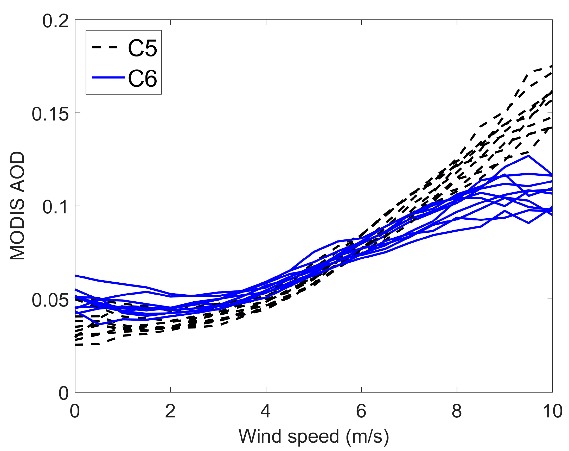
3.7. Comparison between MODIS Collections 5 and 6

MODIS aerosol products are organized according to different collections consisting of data that were generated by different versions of the retrieval algorithms. When comparing Collection 5 (C5) and C6, a significant difference in the AOD-wind speed relationship appears. Figure 11 shows C5 and C6 AOD versus surface wind speed, averaged with respect to autumn (September, October and November) of the period 2003–2012. AOD appears to be more sensitive to surface-wind speed in C5 and it does not show the decrease in AOD at about 9 m/s as with C6 and all the relationships obtained in the previous studies. One likely reason for this is that the modified algorithm overestimate the effect of foam on the water surface at the higher wind speeds. Overall, the present results are consistent with the relationship found between MODIS AOD and wind speed by Levi et al. [43], who highlighted that the C6 algorithm retrieves lower (higher) values of AOD than the C5 when wind speed is higher (lower) than 6 m/s. Thus, the actual relationship between AOD and surface wind speed is likely somewhat stronger that the one obtained here with the C6 algorithm. On the other hand, since MODIS AOD is in this study related to surface wind speed at 2 m, the relationship will be weaker when transforming the relationship to wind speeds at 10 m. The latter can be performed by applying the wind-profile power law:

$$\mathrm{U}={\mathrm{U}}_{\mathrm{r}}(\frac{Z}{z_r}){}^{\alpha }$$

(3)

where U is the wind speed (m/s) at height z (m); U_r is the known wind speed at a reference height z_r; and α is an empirically derived coefficient, which is ~0.11 for open water.

4. Discussion

AOD derived from MODIS Aqua observations over the central North Pacific has been validated against AOD obtained from sun-photometer measurements carried out at three marine ground-based stations and during several ship cruises. MODIS 555 nm AOD was found to vary within the expected uncertainties of the MODIS retrievals over the ground-based sites and ship tracks for 71% and 75%, respectively, of the compared cases. Figure 2 shows that many of the MODIS AOD values are substantially higher than the expected error envelopes. The largest deviation is found in the comparison between MODIS and MAN AOD, where MODIS AOD in some cases exceeds AERONET AOD by almost a factor of 2. When investigating the largest deviation in Figure 2b we found that the AOD values outside the estimated uncertainties ranges belong to nine ship cruises of the 15 in Table 1. Thus, there is not a ship track that stands out concerning the deviation. Another possible cause for the deviation is cloud contamination. Several studies [28,44,59,60,61] found that MODIS tends to overestimate AOD compared to AERONET over ocean areas under cloudy conditions. Zhang et al. [62] analyzed cloud artifacts over remote oceans and found that cloud contamination explains 60–90% of the correlation between MODIS AOD and cloud fraction. Similar deviation as the one found here in MODIS AOD derived from observations over the current coastal sites has also been reported in previous studies [43,63,64,65,66]. Mélin et al. [64] suggest that further improvements of atmospheric correction in coastal waters may require an additional level of detail to describe the complex aerosol mixtures more accurately, and specific water bio-optical models for an appropriate representation of the boundary condition.

The radiance leaving the ocean surface may also cause overestimation in MODIS AOD. An extreme situation is sun glint phenomenon that occurs when sunlight reflects off the surface of water at the same angle than the satellite sensor views it. Although a screening of this effect is included in the MODIS algorithm, in any case it may induce uncertainties in the final product. White foam (whitecap) formations, especially during higher wind-speed conditions, may also induce uncertainties in MODIS-derived AOD. Levi et al. [43] state that despite the improvement in the MODIS Collection 6 algorithm, the errors caused by surface brightness may still have a large impact on the AOD estimated, particularly for cases with relatively low AOD values such as in the marine background atmosphere. Even so, the variability in AOD for the different wind speeds, shown in Figure 3, is in any case relatively constant around the mean values.

Substantially higher MODIS and AERONET (Mauna Loa) AODs were found in the present study for spring compared to the other seasons investigated. These results seem to be consistent with previous studies, e.g., [67,68,69,70]. They all found that trans-Pacific transport of air pollutants from China is most efficient in spring due to active cyclonic activity. Frequent convection in spring lifts particulate matter from the Asian continent to the free troposphere, where prevailing westerlies rapidly transport aerosols across the ocean. When continental air reaches the high-pressure system in the North Pacific, it subsides in the middle troposphere where aerosol residence time is much longer than in the boundary layer. A number of studies [71,72,73,74,75] have also found mineral dust transport from Asia over the North Pacific in spring. In addition, the present back-trajectory analysis suggests a frequent transport of air masses from Asia to the investigation area also in winter, actually most obvious during this season (Figure 8). However, the vertical transport of aerosols from the Asian boundary layer to the free troposphere in winter is expected to be rather limited due to suppressed convection. This means that the transport of aerosols over the North Pacific in winter mainly takes place in the boundary layer, where efficient wet deposition of the aerosols is expected [71].

The AOD dependence on wind speed estimated in the current study is in reasonable agreement with the parameterization derived by Mulcahy et al. [36], although the latter relationship is slightly stronger. AOD derived from the PFR measurements is assumed to be more accurate than AOD derived from MODIS observations. Furthermore, the analysis by Mulcahy et al. [36] was done for selected days that fall into the category of “stable wind conditions”, which are defined as days with the lowest variability in daily wind speeds (less than 2 m/s). At the end, only 14 days were left for analyzing the AOD-wind speed dependence. It is remarkable that the present averaged AOD-wind speed relationship derived from MODIS Aqua observations over the central North Pacific over 14 years are relatively close to the relationship found at Mace Head, since the two studies focused on different oceans with large differences in wind patterns (trade versus westerly winds) and sea-surface temperatures. Note however that the relationship found at Mace Head by Mulcahy et al. (2008) is obtained for substantially higher wind speeds (obtained with 2-min time resolution) than the present relationship. Even so, the majority of the MODIS AOD values over the central North Pacific were derived at a wind speed of around 6 m s⁻¹ and there are probably not many places on Earth that have a mean wind speed substantially higher than 10 m s⁻¹. Although the surface wind speed is the most important factor for determining sea spray aerosol production over ice-free water surfaces, the water temperature plays an important role as well [11,16,17]. Therefore, using the present relationship between AOD and surface-wind speed over other regions on Earth, where the surface-water temperature is substantially lower, induces uncertainties in the estimates of AOD

5. Conclusions

This study shows relatively strong relationships between MODIS mean AOD and surface-wind speed over the central North Pacific for marine background conditions in summer, fall and winter in the period 2003–2016. In addition, the enhanced AOD, due to increased wind speeds, is mainly associated with coarse-mode aerosols. Thus, AOD associated with particles larger than 0.25 μm in radius increases substantially for wind speeds higher than about 3.5 m/s, while only a minor increase is found for the fine-mode aerosols. This is consistent with a fine mode of secondary aerosols that form independent of the wind speed.

To summarize, the current study shows a distinct increase in MODIS AOD for higher wind speeds. The present results show that MODIS Aqua retrievals of AOD in the marine atmosphere agree reasonably well with ground-based remote-sensing observations. To our knowledge, the established parameterization is derived for the longest period of MODIS Aqua observations over the ocean. It can serve as a promising reference for future investigations of the AOD–wind speed relationship.

References

1. Lewis, E.R.; Schwartz, S.E. Sea Salt Aerosol Production: Mechanisms, Methods, Measurements and Models—A Critical Review; American Geophysical Union: Washington, DC, USA, 2004. [Google Scholar]
2. Kieber, D.J.; Keene, W.C.; Frossard, A.A.; Long, M.S.; Maben, J.R.; Russell, L.M.; Kinsey, J.D.; Tyssebotn, I.M.B.; Quinn, P.K.; Bates, T.S. Coupled ocean atmosphere loss of marine refractory dissolved organic carbon. Geophys. Res. Lett. 2016, 43, 2765–2772. [Google Scholar] [CrossRef]
3. Haywood, J.; Ramaswamy, V.; Soden, B. Tropospheric aerosol climate forcing in clear sky satellite observation over the oceans. Science 1999, 283, 1299–1303. [Google Scholar] [CrossRef] [PubMed]
4. Grini, A.; Myhre, G.; Sundet, J.K.; Isaksen, I.S.A. Modeling the annual cycle of sea salt in the Global 3D Model Oslo CTM2, concentrations, fluxes and radiative impact. J. Clim. 2002, 15, 1717–1730. [Google Scholar] [CrossRef]
5. Dobbie, S.; Li, J.; Harvey, R.; Chylek, P. Sea-salt optical properties and GCM forcing at solar wavelengths. Atmos. Res. 2003, 65, 211–233. [Google Scholar] [CrossRef]
6. Ayash, T.; Gong, S.; Jia, C.Q. Direct and indirect shortwave radiative effects of sea salt aerosols. J. Clim. 2008, 21, 3207–3220. [Google Scholar] [CrossRef]
7. Struthers, H.; Ekman, A.M.L.; Glantz, P.; Iversen, T.; Kirkevåg, A.; Mårtensson, E.M.; Seland, Ø.; Nilsson, E.D. The effect of sea ice loss on sea salt aerosol concentrations and the radiative balance in the Arctic. Atmos. Chem. Phys. 2011, 11, 3459–3477. [Google Scholar] [CrossRef]
8. Pierce, J.R.; Adams, P.J. Global evaluation of CCN formation by direct emission of sea salt and growth of ultrafine sea salt. J. Geophys. Res. 2006, 111, D06203. [Google Scholar] [CrossRef]
9. Fan, T.; Toon, O.B. Modeling sea-salt aerosol in a coupled climate and sectional microphysical model: Mass, optical depth and number concentration. Atmos. Chem. Phys. 2011, 11, 4587–4610. [Google Scholar] [CrossRef] [Green Version]
10. Nilsson, E.D.; Rannik, Ü.; Swietlicki, E.; Leck, C.; Aalto, P.P.; Zhou, J.; Norman, M. Turbulent aerosol fluxes over the Arctic Ocean 2. Wind driven sources from the sea. J. Geophys. Res. 2001, 106, 32139–32154. [Google Scholar] [CrossRef]
11. Mårtensson, E.M.; Nilsson, E.D.; de Leeuw, G.; Cohen, L.H.; Hansson, H.C. Laboratory simulations and parameterization of the primary marine aerosol production. J. Geophys. Res. 2003, 108, 4297. [Google Scholar] [CrossRef]
12. Glantz, P.; Svensson, G.; Noone, K.J.; Osborne, S.R. Sea-salt aerosols over the Northeast Atlantic: Model simulations of ACE-2 2nd Lagrangian experiment. Q. J. R. Meteorol. Soc. 2004, 130, 2191–2215. [Google Scholar] [CrossRef]
13. De Leeuw, G.; Andreas, E.L.; Anguelova, M.D.; Fairall, C.W.; Lewis, E.R.; O’Dowd, C.; Schulz, M.; Schwartz, S.E. Production flux of sea spray aerosol. Rev. Geophys. 2011, 49, RG2001. [Google Scholar] [CrossRef]
14. Lundgren, K.B.; Vogel, H.; Kottmeier, C. Direct radiative effects of sea salt for the Mediterranean region under conditions of low to moderate wind speeds. J. Geophys. Res. Atmos. 2013, 118, 1906–1923. [Google Scholar] [CrossRef]
15. Geever, M.; O’Dowd, C.; van Ekeren, S.; Flanagan, R.; Nilsson, D.; de Leeuw, G.; Rannik, U. Sub-micron sea-spray fluxes. Geophys. Res. Lett. 2005, 32, L15810. [Google Scholar] [CrossRef]
16. Salter, M.E.; Nilsson, E.D.; Butcher, A.; Merete, B. On the seawater temperature dependence of continuous plunging jet derived sea spray aerosol. J. Geophys. Res. Atmos. 2014, 119, 9052–9072. [Google Scholar] [CrossRef]
17. Salter, M.E.; Zieger, P.; Acosta Navarro, J.C.; Grythe, H.; Kirkevag, A.; Rosati, B.; Riipinen, I.; Nilsson, E.D. An empirically derived inorganic sea spray source function incorporating sea surface temperature. Atmos. Chem. Phys. 2015, 15, 11047–11066. [Google Scholar] [CrossRef] [Green Version]
18. Woodcock, A.H.; Gilford, M.M. Sampling atmospheric sea salt. Marine Res. 1948, 8, 177–197. [Google Scholar]
19. Blanchard, D.C. The production, distribution and bacterial enrichment of the sea-salt aerosol. In The Air-Sea Exchanges of Gases and Particles; Liss, P.S., Slinn, W.G.N., Eds.; D. Reidel: Norwell, MA, USA, 1983; pp. 407–454. [Google Scholar]
20. Monahan, E.C.; Spiel, D.E.; Davidson, K.L. A model of marine aerosol generation via whitecaps and wave disruption. In Oceanic Whitecaps; Monahan, E.C., MacNiochaill, G., Eds.; D. Reidel: Norwell, MA, USA, 1986; pp. 167–193. [Google Scholar]
21. Nicholls, S. The dynamics of stratocumulus–aircraft observations and comparisons with a mixed layer model. Q. J. R. Meteorol. Soc. 1984, 110, 783–820. [Google Scholar] [CrossRef]
22. Bretherton, C.S.; Austin, P.; Siems, S.T. Cloudiness and marine boundary layer dynamics in the ASTEX Lagrangian experiments. Part II: Cloudiness, drizzle, surface fluxes and entrainment. J. Atmos. Sci. 1995, 52, 2724–2735. [Google Scholar] [CrossRef]
23. Johnson, D.W.; Osborne, S.; Wood, R.; Suhre, K.; Quinn, P.K.; Bates, T.S.; Andreae, M.O.; Noone, K.; Glantz, P.; Bandy, B.; et al. Observations of the evolution of the aerosol, cloud and boundary layer characteristics during the 1st ACE-2 Lagrangian experiment. Tellus 2000, 52B, 348–376. [Google Scholar] [CrossRef]
24. Osborne, S.R.; Johnson, D.W.; Wood, R.; Bandy, B.J.; Andreae, M.O.; O’Dowd, C.D.; Glantz, P.; Noone, K.; Gerbig, C.; Rudolph, J.; et al. Evolution of the aerosol, cloud and boundary layer dynamic and thermodynamic characteristics during the second Lagrangian experiment of ACE-2. Tellus 2000, 52B, 375–400. [Google Scholar] [CrossRef]
25. Wood, R.; Johnson, D.; Osborne, S.; Andreae, M.O.; Bandy, B.; Bates, T.; O’Dowd, C.; Glantz, P.; Noone, K.; Quinn, P.; et al. Boundary layer and aerosol evolution during the 3rd Lagrangian experiment of ACE-2. Tellus 2000, 52B, 239–257. [Google Scholar]
26. Clarke, A.D.; Uehara, T.; Porter, J.N. Lagrangian evolution of an aerosol column during the Atlantic Stratocumulus Transition Experiment. J. Geophys. Res. 1996, 101, 4351–4362. [Google Scholar] [CrossRef]
27. Gong, S.L.; Bartie, L.A.; Blanchet, J.P. Modeling sea-salt aerosols in the atmosphere. Model development. J. Geophys. Res. 1997, 102, 3805–3818. [Google Scholar] [CrossRef]
28. Reid, J.S.; Brooks, B.; Crahan, K.K.; Hegg, D.A.; Eck, T.F.; O’Neill, N.; de Leeuw, G.; Reid, E.A.; Anderson, K.D. Reconciliation of coarse mode sea-salt aerosol particle size measurements and parameterizations at a subtropical ocean receptor site. J. Geophys. Res. 2006, 111, D02202. [Google Scholar] [CrossRef]
29. Textor, C.; Schulz, M.; Guibert, S.; Kinne, S.; Balkanski, Y.; Bauer, S.; Berntsen, T.; Berglen, T.; Boucher, O.; Chin, M.; et al. Analysis and quantification of the diversities of aerosol life cycles within AeroCom. Atmos. Chem. Phys. 2006, 6, 1777–1813. [Google Scholar] [CrossRef]
30. Glantz, P.; Bourassa, A.; Herber, A.; Iversen, T.; Karlsson, J.; Kirkevåg, A.; Maturilli, M.; Seland, Ø.; Stebel, K.; Struthers, H.; et al. Remote sensing of aerosols in the Arctic for an evaluation of global climate model simulations. J. Geophys. Res. 2014, 119, 8169–8188. [Google Scholar] [CrossRef] [Green Version]
31. Grythe, H.; Ström, J.; Krejci, R.; Quinn, P.; Stohl, A. A review of sea-spray aerosol source functions using a large global set of sea salt aerosol concentration measurements. Atmos. Chem. Phys. 2014, 14, 1277–1297. [Google Scholar] [CrossRef] [Green Version]
32. Smirnov, A.; Holben, B.N.; Eck, T.F.; Dubovik, O.; Slutsker, I. Effect of wind speed on columnar aerosol optical properties at Midway Island. J. Geophys. Res. 2003, 108, 4802. [Google Scholar] [CrossRef]
33. Lehahn, Y.; Koren, I.; Boss, E.; Ben-Ami, Y.; Altaratz, O. Estimating the maritime component of aerosol optical depth and its dependency on surface wind speed using satellite data. Atmos. Chem. Phys. 2010, 10, 6711–6720. [Google Scholar] [CrossRef]
34. Huang, H.; Thomas, G.E.; Grainger, R.G. Relationship between wind speed and aerosol optical depth over remote ocean. Atmos.Chem. Phys. 2010, 10, 5943–5950. [Google Scholar] [CrossRef]
35. Kiliyanpilakkil, V.P.; Meskhidze, N. Deriving the effect of wind speed on clean maritime aerosol optical properties using the A-Train satellites, Atmos. Chem. Phys. Discuss. 2011, 11, 4599–4630. [Google Scholar] [CrossRef]
36. Mulcahy, J.P.; O’Dowd, C.D.; Jennings, S.D.; Ceburnus, D. Significant enhancement of aerosol optical depth in marine air under high wind conditions. Geophys. Res. Lett. 2008, 35, L16810. [Google Scholar] [CrossRef]
37. Glantz, P.; Nilsson, E.D.; von Hoyningen-Huene, W. Estimating a relationship between aerosol optical thickness and surface wind speed over the ocean. Atmos. Res. 2009, 92, 58–68. [Google Scholar] [CrossRef]
38. Satheesh, S.; Moorthy, K. Contribution of sea-salt to aerosol optical depth over the Arabian Sea derived from MODIS observations. Geophys. Res. Lett. 2006, 33. [Google Scholar] [CrossRef]
39. Tanré, D.; Kaufman, Y.J.; Herman, M.; Mattoo, S. Remote sensing of aerosol properties over oceans using the MODIS/EOS spectral radiances. J. Geophys. Res.-Atmos. 1997, 102, 16971–16988. [Google Scholar]
40. Levy, R.C.; Remer, L.A.; Tanré, D.; Kaufman, Y.J.; Ichoku, C.; Holben, B.N.; Livingston, J.M.; Russel, P.B.; Maring, M. Evaluation of the MODIS retrievals of dust aerosol over the ocean during PRIDE. J. Geophys. Res. 2003, 108, 8594. [Google Scholar] [CrossRef]
41. Levy, R.; Remer, L.A.; Dubovik, O. Global aerosol optical properties and application to MODIS aerosol retrieval over land. J. Geophys. Res. 2007, 112, D13210. [Google Scholar] [CrossRef]
42. Levy, R.C.; Remer, L.A.; Kleidman, R.G.; Mattoo, S.; Ichoku, C.; Kahn, R.; Eck, T.F. Global evaluation of the Collection 5 MODIS dark-target aerosol products over land. Atmos. Chem. Phys. 2010, 10, 10399–10420. [Google Scholar] [CrossRef] [Green Version]
43. Levy, R.C.; Mattoo, S.; Munchak, L.A.; Remer, L.A.; Sayer, A.M.; Patadia, F.; Hsu, N.C. The Collection 6 MODIS aerosol products over land and ocean. Atmos. Meas. Tech. 2013, 6, 2989–3034. [Google Scholar] [CrossRef]
44. Remer, L.A.; Kaufman, Y.J.; Tanre, D.; Mattoo, S.; Chu, D.A.; Martins, J.V.; Li, R.R.; Ichoko, C.; Levy, R.C.; Kleidman, R.G.; et al. The MODIS aerosol algorithm, products, and validation. J. Atmos. Sci. 2005, 62, 947–973. [Google Scholar] [CrossRef]
45. Holben, B.N.; Eck, T.F.; Slutsker, I.; Tanre, D.; Buis, J.P.; Setzer, A.; Vermote, E.F.; Reagan, J.A.; Kaufman, Y.J.; Nakajima, T.; et al. AERONET—A federated instrument network and data archive for aerosol characterization. Remote Sens. Environ 1998, 66, 1–16. [Google Scholar] [CrossRef]
46. Smirnov, A.; Holben, B.N.; Slutsker, I.; Giles, D.M.; McClain, C.R.; Eck, T.F.; Sakerin, S.M.; Macke, A.; Croot, P.; Zibordi, G.; et al. Maritime Aerosol Network as a component of Aerosol Robotic Network. J. Geophys. Res. 2009, 114, D06204. [Google Scholar] [CrossRef]
47. Garza, J.A.; Chu, P.; Norton, C.W.; Schroeder, T.A. Changes of the prevailing trade winds over the islands of Hawaii and the North Pacific. J. Geophys. Res. 2012, 117, D11109. [Google Scholar] [CrossRef]
48. Stohl, A.; Wotawa, G.; Seibert, P.; Kromp-Kolb, H. Interpolation errors in wind fields as a function of spatial and temporal resolution and their impact on different types of kinematic trajectories. J. Appl. Metereol. 1995, 34, 2149–2165. [Google Scholar] [CrossRef]
49. Stohl, A.; Seibert, P. Accuracy of trajectories as determined from the conservation of meteorological tracers. Q. J. R. Meteorol. Soc. 1998, 125, 1465–1484. [Google Scholar] [CrossRef]
50. Mishchenko, M.I.; Liu, L.; Geogdzhayev, I.V.; Travis, L.D.; Cairns, B.; Lacis, A.A. Toward unified satellite climatology of aerosol properties. 3. MODIS versus MISR versus AERONET. J. Quant. Spectrosc. Radiat. Transf. 2010, 111, 540–552. [Google Scholar] [CrossRef]
51. Monahan, E.C.; O’Muircheartaigh, I. Optimal power-law description of oceanic whitecap coverage dependence on wind speed. J. Phys. Oceanogr. 1980, 10, 2094–2099. [Google Scholar] [CrossRef]
52. Callaghan, A.; de Leeuw, G.; Cohen, L.; O’Dowd, C.D. Relationship of oceanic whitecap coverage to wind speed and wind history. Geophys. Res. Lett. 2008, 35, L23609. [Google Scholar] [CrossRef]
53. Norris, S.J.; Brooks, I.M.; Moat, B.I.; Yelland, M.J.; de Leeuw, G.; Pascal, R.W.; Brooks, B. Near-surface measurements of sea spray aerosol production over whitecaps in the open oceam. Ocean. Sci. 2013, 9, 133–145. [Google Scholar] [CrossRef]
54. Albert, M.F.M.A.; Anguelova, M.D.; Manders, A.M.M.; Schaap, M.; de Leeuw, G. Parameterization of oceanic whitecap fraction based on satellite observations. Atmos. Chem. Phys. 2016, 16, 13725–13751. [Google Scholar] [CrossRef]
55. Smirnov, A.; Sayer, A.M.; Holben, B.N.; Hsu, N.C.; Sakerin, S.M.; Macke, A.; Nelson, B.B.; Courcoux, Y.; Smyth, T.J.; Croot, P.; et al. Effect of wind speed on aerosol optical depth over remote oceans, based on data from the Maritime Aerosol, Network. Atmos. Meas. Tech. 2012, 5, 377–388. [Google Scholar] [CrossRef] [Green Version]
56. O’Dowd, C.D.; Scannell, C.; Mulcahy, J.; Jennings, S.G. Wind speed influences on marine aerosol optical depth. Adv. Meteorol. 2010. [Google Scholar] [CrossRef]
57. Shinozuka, Y.; Clarke, A.D.; Howell, S.G.; Kapustin, V.N.; Huebert, B.J. Sea-salt vertical profiles over the Southern and tropical Pacific oceans: Microphysics, optical properties, spatial variability, and variations with wind speed. J. Geophys. Res. 2004, 109, D24201. [Google Scholar] [CrossRef]
58. Wu, J. Oceanic Whitecaps and Sea State. J. Phys. Oceanogr. 1979, 9, 1064–1068. [Google Scholar] [CrossRef]
59. Ichoku, C.; Chu, D.A.; Mattoo, S.; Kaufman, Y.J.; Remer, L.A.; Tanré, D.; Slutsker, I.; Holben, B.N. A spatio-temporal approach for global validation and analysis of MODIS aerosol products. Geophys. Res. Lett. 2002, 29, 8006. [Google Scholar] [CrossRef]
60. Zhang, J.; Reid, J.S. MODIS aerosol product analysis for data assimilation: Assessment of over-ocean level 2 aerosol optical thickness retrievals. J. Geophys. Res. 2006, 111, D22207. [Google Scholar] [CrossRef]
61. Shi, Y.; Zhang, J.; Reid, J.S.; Holben, B.; Hyer, E.J.; Curtis, C. An analysis of the collection 5 MODIS over-ocean aerosol optical depth product for its implication in aerosol assimilation. Atmos. Chem. Phys. 2011, 11, 557–565. [Google Scholar] [CrossRef] [Green Version]
62. Zhang, J.; Reid, J.; Holben, B. An analysis of potential cloud artifacts in MODIS over ocean aerosol optical thickness products. Geophys. Res. Lett. 2005, 32, L15803. [Google Scholar] [CrossRef]
63. Mélin, F. Comparison of SeWiFS and MODIS time series of inherent properties for the Adriatic Sea. Ocean. Sci. 2011, 7, 351–361. [Google Scholar] [CrossRef]
64. Mélin, F.; Zibordi, G.; carlund, T.; Holben, B.N.; Stefan, S. Validation of SeaWiFS and MODIS Aqua/Terra aerosol products in coastal regions of European marginal seas. Oceanologia 2013, 55, 27–51. [Google Scholar] [CrossRef]
65. Tesche, M.; Glantz, P.; Johansson, C. Spaceborne observations of low surface aerosol concentrations in the Stockholm region. Tellus B 2016, 68, 28951. [Google Scholar] [CrossRef]
66. Glantz, P.; Freud, E.; Johansson, C.; Tesche, M. Trends in MODIS and AERONET derived aerosol optical thickness over Northern Europe. Tellus 2018. under review. [Google Scholar]
67. Forster, C.; Cooper, O.; Stohl, A.; Eckhardt, S.; James, P.; Dunlea, E.; Nicks, D.K., Jr.; Holloway, J.S.; Hubler, G.; Parrish, D.D.; et al. Lagrangian transport model forecasts and a transport climatology for the Intercontinental Transport and Chemical Transformation 2002 (ITCT 2K2) measurement campaign. J. Geophys. Res. 2004, 109, D07S92. [Google Scholar] [CrossRef]
68. Liang, Q.; Jaegle, L.; Jaffe, D.A.; Weiss-Penzias, P.; Heckman, A.; Snow, J.A. Long range transport of Asian pollution to the northeast Pacific: Seasonal variations and transport pathways of carbon monoxide. J. Geophys. Res. 2004, 109, D23S07. [Google Scholar] [CrossRef]
69. Heald, C.L.; Jacob, D.J.; Park, R.J.; Alexander, B.; Fairlie, T.D.; Yantosca, R.M.; Chu, D.A. Transpacific transport of Asian anthropogenic aerosols and its impact on surface air quality in the United States. J. Geophys. Res. 2006, 111, Dl4310. [Google Scholar] [CrossRef]
70. Yu, H.; Chin, M.; Remer, L.; Kleidman, R.G.; Bellouin, N.; Bian, H.; Diehl, T. Variability of marine aerosol fine-mode fraction and estimates of anthropogenic aerosol component over cloud-free oceans from the Moderate Resolution Imaging Spectroradiometer (MODIS). J. Geophys. Res. 2009, 114, D10206. [Google Scholar] [CrossRef]
71. Darzi, M.; Winchester, J.W. Resolution of basaltic and continental aerosol components during spring and summer within the boundary layer of Hawaii. J. Geophys. Res. 1982, 87, 7262–7272. [Google Scholar] [CrossRef]
72. Uematsu, D.R.A.; Prospero, J.M.; Chen, L.; Merrill, J.T.; McDonald, R.L. Transport of mineral aerosol from Asia over the North Pacific Ocean. J. Geophys. Res. 1983, 88, 5343–5352. [Google Scholar] [CrossRef]
73. Takemura, T.; Nakajima, T.; Dubovik, O.; Holben, B.N.; Kinne, S. Single-scattering albedo and radiative forcing of various aerosol species with a global three-dimensional model. J. Clim. 2002, 15, 333–352. [Google Scholar] [CrossRef]
74. Chin, M.; Diehl, T.; Ginoux, P.; Malm, W. Intercontinental transport of pollution and dust aerosols: Implications for regional air quality. Atmos. Chem. Phys. Disccuss. 2007, 7, 9013–9051. [Google Scholar] [CrossRef]
75. Huang, J.; Minnis, P.; Chen, B.; Huang, Z.; Liu, Z.; Zhao, Q.; Yi, Y.; Ayers, K.J. Long-range transport and vertical structure of Asian dust from CALIPSO and surface measurements during PACDEX. J. Geophys. Res. 2008, 113, D23212. [Google Scholar] [CrossRef]
Figure 1. The investigation area (12° N–35° N, 145° W–168° W) in the central North Pacific is shown in (b) and denoted with a black box in (a). Aerosol optical depths (AODs) were derived based on MODIS Aqua observations on 18 September 2014 (right). Aerosol Robotic Network (AERONET) ground-based data were obtained from the stations at Coconut Island (21.4° N, 157.8° W) and Lanai (20.7° N, 156.9° W) on Hawaii, as well as from Midway (28.2° N, 177.4° W) west of the investigation area (orange solid circle in (a)).
Atmosphere 09 00060 g001
Figure 2. (a) Comparison between Moderate Resolution Imaging Spectroradiometer (MODIS) and AERONET AOD; and (b) MODIS and MAN AOD at 555 nm. The solid and dashed lines represent the 1-to-1 line and estimated uncertainties of the MODIS retrievals over ocean (ΔAOD = +0.04 + 0.1·AOD, ΔAOD = −0.02 − 0.1·AOD), respectively. Error bars correspond to the MODIS/AERONET and MODIS/MAN AODs’ comparison and denote one standard deviation.
Atmosphere 09 00060 g002
Figure 3. MODIS-adjusted AOD (grey dots) on pixel basis versus surface wind speed for summer 2007. The grey solid circles denote the median AOD and corresponding median absolute deviation for the binned data. The black solid and red dashed lines denote a power fit and corresponding 95% confidence interval, respectively. The R2 and RMSE values were calculated based on the power fit of the median values.
Atmosphere 09 00060 g003
Figure 4. MODIS-adjusted median AOD (555 nm) versus surface wind speed, subdivided with respect to season, for each year of the period 2003–2016. The orange solid line in each figure denote MODIS mean AOD, averaged over the investigation period.
Atmosphere 09 00060 g004
Figure 5. Frequency distributions of all AOD, derived from observations over the Northern Pacific during the period 2003–2016, which have been normalized with respect to the total number of derived AOD corresponding to the (a) season and (b) year.
Atmosphere 09 00060 g005
Figure 6. (a) Mean Ångström exponent, derived from MODIS Aqua observations over the period 2003–2016, versus surface wind speed and subdivided according to season; (b) MODIS Aqua fine mode adjusted median AOD (thin lines) and total adjusted median AOD (bold lines) obtained for different seasons of the period 2003–2016 versus surface wind speed.
Atmosphere 09 00060 g006
Figure 7. Bold and thin solid line denote daily mean AOD and corresponding one standard deviation, respectively, obtained from yearly time series observed at the AERONET Mauna Loa station during the period 2003–2016.
Atmosphere 09 00060 g007
Figure 8. FLEXible TRAjectories (FLEXTRA) ECMWF 7-day back-trajectories starting at Mauna Loa (19.54° N, 155.58° W), Hawaii, at a height of 3000 m above sea level, subdivided with respect to (a) winter; (b) spring; (c) summer and (d) fall. Color shading denotes the probability of occurrence for air masses passing over a particular grid-cell before they arrived at Mauna Loa (see explanation in the text).
Atmosphere 09 00060 g008
Figure 9. MODIS-adjusted mean AOD (black solid circle) with corresponding one standard deviation, averaged with respect to the median annual curves obtained for summer, fall and winter in Figure 4. The blue solid line is a power-law fit of the mean AOD values.
Atmosphere 09 00060 g009
Figure 10. The present relationship between adjusted AOD and surface-wind speed in comparison to relationships obtained in previous studies. More information is given in Table 2.
Atmosphere 09 00060 g010
Figure 11. MODIS C5 and C6 AOD (black dashed and blue solid lines, respectively) versus surface wind speed, averaged with respect to September, October and November for the years 2003–2012.
Atmosphere 09 00060 g011