Evaluation of Analysis by Cross-Validation, Part II: Diagnostic and Optimization of Analysis Error Covariance


Air Quality Research Division, Environment and Climate Change Canada, 2121 Transcanada Highway, Dorval, QC H9P 1J3, Canada
*
Author to whom correspondence should be addressed.
Atmosphere 2018, 9(2), 70; https://doi.org/10.3390/atmos9020070
Submission received: 7 November 2017
/
Revised: 19 January 2018
/
Accepted: 13 February 2018
/
Published: 15 February 2018
(This article belongs to the Special Issue Air Quality Monitoring and Forecasting)
Abstract
:We present a general theory of estimation of analysis error covariances based on cross-validation as well as a geometric interpretation of the method. In particular, we use the variance of passive observation-minus-analysis residuals and show that the true analysis error variance can be estimated, without relying on the optimality assumption. This approach is used to obtain near optimal analyses that are then used to evaluate the air quality analysis error using several different methods at active and passive observation sites. We compare the estimates according to the method of Hollingsworth-Lönnberg, Desroziers et al., a new diagnostic we developed, and the perceived analysis error computed from the analysis scheme, to conclude that, as long as the analysis is near optimal, all estimates agree within a certain error margin.
1. Introduction
At Environment and Climate Change Canada (ECCC) we have been producing hourly surface pollutants analyses covering North America [1,2,3] using an optimum interpolation scheme which combines the operational air quality forecast model GEM-MACH output [4] with real-time hourly observations of O3, PM2.5, PM10, NO2, and SO2 from the AirNow gateway with additional observations from Canada. These analyses are not used to initialize the air quality model and we wish to evaluate them by cross-validation, that is by leaving out a subset of observations from the analysis to use them for verification. Observations used to produce the analysis are called active observations while those used for verification are called passive observations.
In a first-part paper of this study, i.e., Ménard and Deshaies-Jacques [5], we have examined different verification metrics using either active or passive observations. As we changed the ratio of observation error to background error variances , while keeping the sum equal to , we found a minimum in in the passive observation space. In this second-part paper, we formalize this result, develop the principles of estimation of the analysis error covariance by cross-validation, and apply it to estimate and optimize the analysis error covariance of ECCC’s surface analyses of O3 and PM2.5.
When we refer to analysis error, or analysis error covariance, it is important to distinguish the perceived analysis error with the true analysis error [6]. The perceived analysis error is the analysis error that results from the analysis algorithm itself, whereas the true analysis error is the difference between the analysis and the true state. Analysis schemes are usually derived from an optimization of some sort. In a variational analysis scheme for example, the analysis is obtained by minimizing a cost function with some given or prescribed observation error and background error covariances, and respectively. In a linear unbiased analysis scheme, the gain matrix is obtained by minimum variance estimation, yielding an expression of the form, , where is the observation operator. The perceived analysis error covariance is then derived as . In order to derive an expression for the perceived analysis error covariance we in fact assume that given error covariances, and , are error covariances with respect to the true state, i.e., the true error covariances. We also assume that the observation operator is not an approximation with some error, but is the true error-free observation operator. Of course, in real applications neither of and are covariance measures with respect to the true state, but only a more or less accurate estimate of those. Daley [6] have argued that in principle for an arbitrary gain matrix , the true analysis error covariance can be computed as provided that we know the true observation and background error covariances, and . This expression is a quadratic matrix equation, and has the property that the true analysis error variance, is minimum when . In that sense, the analysis is truly optimal. The optimal gain matrix is called the Kalman gain. It thus illustrates that although an analysis is obtained through some minimization principle, the resulting analysis error is not necessarily the true analysis error.
One of the main sources of information to obtain the true and is from the statistic. However, it has always been argued that this is not possible without making some assumptions [7,8,9], the most useful one being that background errors are spatially correlated while the observation errors are spatially uncorrelated, or at least on a much shorter length-scale. Even under those assumptions, different estimation methods such as the Hollingsworth-Lönnberg method [10], the maximum likelihood gives different error variances and different correlation lengths [11]. Other methods use for rescaling but assume that the observation error is known. The assumption that the observation error is known is also debated as they contain representativeness errors [12] that include observation operator errors. How to obtain an optimal analysis is thus unclear.
The evaluation of the true or perceived analysis error covariance using its own active observations is also a misleading problem unless the analysis is already optimal. Hollingsworth and Lönnberg [13] addressed this issue for the first time where they noted that in the case of an optimal gain (i.e., optimal analysis), the statistics of observation-minus-analysis residuals are related to the analysis error by , where is the optimal analysis error covariance and and are the observation operator and observation error covariance respectively. The caret (^) over indicates that the analysis uses an optimal gain. In the context of spatially uncorrelated observation errors, the off-diagonal elements of would then give the analysis error covariance in observation space. Hollingsworth and Lönnberg [13] argued that for most practical purposes, the negative intercept of at zero distance and the prescribed observation weight should be nearly equal, and thus could be used as an assessment of optimality of an analysis. However, in case where such agreement does not exist, an estimate of the actual analysis error is not possible. Another method, proposed by Desroziers et al. [14], argued that the diagnostic should be equal to the analysis error covariance in observation space but, again, only if the gain is optimal and the innovation covariance consistency is respected [15].
The impasse of the estimation of the true analysis error seems to be tied with using active observations, i.e., using the same observations as those used to create the analysis. A robust approach that does not require an optimal analysis is to use observations whose errors are uncorrelated with the analysis error. For example, if we assume that observation errors are temporarily (serially) uncorrelated, an estimation of the analysis error can be made with the help of a forecast model initialized by the analysis by verifying the forecast against these observations. This is the essential assumption used traditionally in meteorological data assimilation to assess indirectly the analysis error by comparing the resulting forecast with observations valid at the forecast time. As forecast error grows with time, the observation-minus-forecast can be used to assess whether an analysis is better than another. In a somewhat different method but making the same assumption, Daley [6] used the temporal (serial) correlation of the innovations to diagnose the optimality of the gain matrix. This property was first established in the context of Kalman filter estimation theory by Kailath [16]. However, both the traditional meteorological forecast approach and the Daley method [6] are subject to limitations: they assume that the model forecast has no bias and the analysis corrections are made correctly on all the variables needed to initialize the model. In practice, improper initialization of unobserved meteorological variables gives rise to spin-up problems or imbalances. Furthermore, with the traditional meteorological approach, compensation due to model error can occur, so that an optimal analysis does not necessarily yield an optimal forecast [7].
An alternative approach introduced by Marseille et al. [17], which we will follow here, is to use independent observation or passive observations to assess the analysis error. The essential assumption of this method is that the observations have spatially uncorrelated errors, so that the observations used for verification, i.e., the passive observations, have uncorrelated errors with the analysis. The advantage of this approach is that it does not involve any model to propagate the analysis information to a later time. Marseille et al. [17] then showed that by multiplying the Kalman gain with an appropriate scalar value, one can reduce the analysis error. In this paper, we go further by using principles of error covariance estimation to obtain a near optimal Kalman gain. In addition we impose the innovation covariance consistency [15] and show that all diagnostics of analysis error variance nearly agree with one another. These include the Hollingsworth and Lönnberg [13], the Desroziers et al. [14] and new diagnostics that we will introduce.
The paper is organized as follows. First we present in Section 2 the theory and diagnostics of analysis error covariance in both passive and active observation spaces, as well as a geometrical representation. This leads us to a method to minimize the true analysis error variance. In Section 3, we present the experimental setup on how we obtain near optimal analyses and presents the results of several diagnostics in active and passive observation spaces, and compare with the analysis error variance obtained from the optimum interpolation scheme itself. In Section 4, we discuss the statistical assumptions being used, how and if they can be extended and how this formalism can be used in other applications such as the estimation of correlated observation errors with satellite observations. Finally, we draw some conclusions in Section 5.
2. Theoretical Framework
This section is composed of mainly three parts. In Section 2.1 and Section 2.2, we first describe the diagnostics to obtain the true error covariances using passive observations whether the analysis is optimal or not. We then give a geometric interpretation in Section 2.3 that indicate the way to obtain the optimal analysis, that is, one that minimizes the true analysis error. Lastly, in Section 2.4 and Section 2.5, we formulate the diagnostics of analysis error for optimal analyses.
2.1. Diagnostic of Analysis Error Covariance in Passive Observation Space
Let us decompose the observation space in two disjoint sets; the active observation set or training set used to create the analysis, and the independent or passive observation set used to evaluate the analysis. An analysis built from prescribed background and observation error covariances, and respectively, is given by
where is the gain matrix built from the prescribed error covariances, is the observation operator for the active observation set, is the active innovation vector, , is the background state or model forecast, is the active observation error and the background error. The observation-minus-analysis residual for the active set is given by [14,15,18].
where is the analysis error. The analysis interpolated at the passive observation sites can be denoted by , where is the observation operator at passive observation sites. The observation-minus-analysis residual at the passive observation sites is then given by
where is the innovation at the passive observation sites. Note that the formalism introduced here is general, and can be used with any set of independent observations such as different instruments or observation networks as long as the operator is properly defined. Consequently, for generality, we distinguish the passive observation errors or independent observation error, , from the active observation error .
There are two important statistical assumptions from which we derive cross-validation diagnostics. Assuming that the observation errors are spatially uncorrelated, it follows that
where is the mathematical expectation that represents the mean over an ensemble of realizations. It has been argued by Marseille et al. [17] that representativeness error can violate this assumption for a close pair of active-passive observations, but we will neglect this effect. Also, assuming that observation errors are uncorrelated with background error, we have
We come now to the most important property: since the analysis is a linear combination of the active observations and the background state, the analysis error is then uncorrelated with the passive observation errors,
and thus we get the following cross-validation diagnostic in passive observation space,
similarly to Marseille et al. [17]. A very important point to note is that is the true analysis error covariance—it does not assume that the gain is optimal. The matrices in Equation (7) are of the dimension of the passive observation space and is the observation error covariance matrix for the passive or independent observations.
2.2. A Complete Set of Diagnostics of Error Covariances in Passive Observation Space
It is also possible to define a set of diagnostics that would determine, in principle, the true error covariances, and . From Equations (4) and (5) we get another cross-validation diagnostic,
This diagnostic is related to the Hollingsworth-Lönnberg [10] estimation of the spatially correlated part of the innovation, and in practice can be dominated by sampling error. Note that it is not a square matrix and an estimation of parameters of B may not be trivial.
We can also obtain the innovation covariance matrix in passive observation space (identical in fact to the one in active observations space) as
The system of Equations (7)–(9) gives a complete set of equations to determine the true and at the passive observation sites provided that by interpolation/extrapolation we can obtain from .
Nevertheless, and for sake of completeness, we also investigated the meaning of the statistics and came to the conclusion that it can interpreted as a misfit to the Desroziers et al. estimate of [14] with the true value . We recall that the first iterate of the Desroziers et al. estimate for in active observation space is given by [15], where we used the superscript D indicate the Desroziers et al. first iterate estimate. We can actually generalize this diagnostic to be a cross-covariance between state space and active observation space as
By applying to Equation (10) we can then introduce a generalized Desroziers et al. estimate of the background error covariance between passive and active observation spaces as,
Since , we get with Equations (8) and (10),
That is the difference between the true and the Desroziers et al. first estimate in the cross passive-active observation spaces. Similarly to Equation (8) this diagnostics requires spatial interpolation of error covariances from active sites to passive sites of basically noisy statistics. The estimation of from this diagnostics is further complicated by the fact that what is being interpolated, that is , may not even be positive definite, but the augmented matrix,
is positive definite. Except for the diagonal of Equation (13), we have not attempted in this study to conduct this complete estimation of and , but rather focused on getting a reliable estimate of the analysis error covariance .
2.3. Geometrical Interpretation
A geometrical illustration of some of the relationships obtained above can be made by using a Hilbert space representation of random variables in observation space. A 2D representation for the analysis of a scalar quantity was used in Desroziers et al. [14] to illustrate their a posteriori diagnostics. We will generalize this approach to include passive observations by considering a 3D representation.
As in Desroziers et al. [14] let’s consider the analysis of a scalar quantity. Several variables are to be considered in this observation space: the active observation (or measurement) of the scalar quantity, the background (or prior) value equivalent in observation space (i.e., ), the analysis in observation space (i.e., ), and for verification an independent observation (or passive observation) that is not used to compute the analysis. Each of these quantities is a random variable as they each contain random errors, and any linear combination of random variables in observation space also belong to observation space. For example, is the innovation (commonly denoted by O-B) and that belongs to observation space, is the analysis increment in observation space (commonly denoted by A-B), and is the analysis residual in observation space (commonly denoted by O-A). We can also define an inner product of any random variables in observation space. , as
The squared norm then represents the variance,
so the inner product has the following geometric interpretation
where is the correlation coefficient. Uncorrelated random variables are thus statistically orthogonal. With this inner product, the observation space forms a Hilbert space of random variables.
Figure 1 illustrates the statistical relationship in observation space between: the active observation (illustrated as O in the figure), the prior or background (i.e., B), the analysis (i.e., A), and the independent observation (i.e., Oc). The origin T corresponds to the truth of the scalar quantity, and also corresponds to the zero of the central moment of each random variables, e.g., , since each variables are assumed to be unbiased. We also assume that the background, active and passive observations errors are uncorrelated to one another, so the three axes; for the active observation error, for the background error, and for the passive observation error are orthogonal. The plane defined by and axes is the space where the analysis takes place, and is called the analysis plane. However, since we define the analysis to be linear and unbiased, only linear combinations of the form where k is a constant are allowed. The analysis A then lies on the line (B, O). The thick lines in Figure 1 represent the norm of the associated error. For example, the thick line along the axis depict the (active) observation standard deviation , and similarly for the other axes and other random variables. Since the active observation error is uncorrelated with the background error, the triangle ΔOTB is a right triangle, and by Pythagoras theorem we have, . This is the usual statement that the innovation variance is the sum of background and observation error variances. The analysis is optimum when the analysis error is minimum, in which case the line is perpendicular to line (O, B).
Now let’s consider the passive observation Oc . The passive observation error is perpendicular to the analysis plane, thus the triangle ΔOcTA is a right triangle,
where is the passive observation error variance. The most important fact to stress here is that the orthogonality expressed in Equation (17) is true whether or not the analysis is optimal. Furthermore, as the distance varies with the position of along the line (O, B), the distance reaches a minimum value when is minimum that is when the analysis is optimal. We thus also argue from this representation that there is always a minimum, and the minimum is unique. Finally, we note that ΔBTOc is also a right triangle so that , which is the scalar version of Equation (9).
To extend this formalism to random vectors requires to define a proper matricial inner product as briefly described in Section 1.2 of Caines [19]. It is important here to distinguish the stochastic metric space from the observation vector space. In the stochastic metric space a “scalar” needs not to be a number, but only a non-random quantity invariant with respect to . Hence, we can define a Hilbert space with the following (stochastic scalar) matricial inner product . The matrix nature of pertains to the observation vector space, but it remains a scalar with respect to the stochastic Hilbert space herein defined. In order to obtain a true scalar (), one would need to define a metric on the observation space matrices as well, such as the trace. Also to be able to compare active and passive observations, projectors need to be introduced on the observation space, implying yet another metric structure on the observation space. We do not carry out this formalism here as it would represent a rather lengthy development that would distract us from the main purpose of this paper; this will be considered in a future manuscript. Finally, we remark that Hilbert space representation of random variables in infinite dimensional space (i.e., continuous space) can also be defined, see Appendix 1 of Cohn [20].
2.4. Error Covariance Diagnostics in Active Observation Space for Optimal Analysis
An analysis is optimal if the analysis error is minimum. This implies that the gain matrix using the prescribed error covariances, in Equation (1), must be identical to the gain using the true error covariances, i.e., [14,15]. It is important to mention that necessary and sufficient conditions to obtain the true error covariances and in observation space, are: 1—the Kalman gain condition, and 2—the innovation covariance consistency, . For a proof see the Theorem on error covariance estimates in Ménard [15].
From the optimality of the analysis (or Kalman gain) alone, we derive that or . Indeed, from Equation (2), we get , and for the analysis error in observation space we get, , from which we derive the expectations above. Using the geometrical representation in Section 2.3 the distance between A and T is minimum, when and (Figure 1) are right triangles. We should also note that for the scalar problem, the Kalman gain depends only on the ratio of observation to background error variances and thus the scalar Kalman gain is optimal if the ratio of the prescribed error variances is equal to the ratio of the true error variances.
If in addition to the optimality of the analysis or Kalman gain we add the innovation covariance consistency then we get three different statistical diagnostics of the (optimal) analysis error covariance. Hollingsworth and Lönnberg [13] was the first to introduce a statistical diagnostic of analysis error in the active observation space, as:
Here we use a subscript, HL to indicate that this is the Hollingsworth-Lönnberg estimate. Equation (18) can obtained from the covariance of and that, for an optimal gain matrix, which derives from the usual formula, . Geometrically it derives from the fact that the triangle is a right triangle, and from the innovation covariance consistency that implies that the triangle is a right triangle. Using data to construct , an estimated analysis error covariance obtained from Equation (18) is symmetric but could be non-positive definite as it is obtained by subtracting two positive definite matrices. The effect of misspecification in the prescribed error covariances resulting from a lack of innovation covariance consistency will be discussed in the result Section 3 and in Appendix B.
Inspired from the geometrical interpretation that is also be a right triangle we derived the following diagnostic,
where MDJ stands for Ménard-Deshaies-Jacques. This relationship is obtained by using the expression , the innovation covariance consistency and the formula for the optimal analysis error covariance . As for the HL diagnostics, the estimated error covariance obtained from this diagnostic is symmetric by construction but may not be positive definite. Another way of looking at Equation (19) is that it expresses, in observation space, the error reduction due to the use of observations.
Another diagnostic of analysis error covariance was proposed by Desroziers et al. [14]. By combining and we get
where the subscript D denotes the Desroziers et al. estimate. By construction, the estimated analysis error covariance is not necessarily symmetric. A geometrical derivation is provided in Appendix A. We also provide in Appendix B a sensitivity analysis on the departure from innovation covariance consistency for each diagnostics in both active and passive observation spaces.
2.5. Error Covariance Diagnostics in Passive Observation Space for Optimal Analysis
We can also derive optimal analysis diagnostics in the passive observation space. Considering the 3D geometric interpretation, and in particular the tetrahedron , we notice that since is a right triangle, so is , which is a projection of the triangle on the plane passing through Oc, O and B. We thus have . Combining this result with Equation (7) and using, , we then get
Note that our analysis diagnostic is the only diagnostic that is valid in both active and passive observation spaces, i.e., Equation (21) is similar to Equation (19).
The other, less direct, diagnostic for optimal analysis is simply based on Equation (7) that is
These five diagnostics will be used later in the results section.
3. Results with Near Optimal Analyses
3.1. Experimental Setup
We will just give here a short summary of the experimental setup we are using in this study. More details can be found in the Part I paper (Ménard and Deshaies-Jacques [5]). A series of hourly analyses of O3 and PM2.5 at 21 UTC for a period of 60 days (14 June to 12 August 2014) were performed using an optimum interpolation scheme combining the operational air quality model GEM-MACH forecast and the real-time AirNow observations (see Section 2 of [5] for further details). The analyses are made off-line so they are not used to initialize the model. As input error covariances, we use uniform observation and background error variances, with and , where is a homogeneous isotropic error correlation based on a second-order autoregressive model. The correlation length is estimated by using a maximum likelihood method using at first, error variances obtained from a local Hollingworth-Lönnberg fit [11] (and only for the purpose of obtaining a first estimate of the correlation length). We then conduct a series of analyses by changing error variance ratio while at the same time respecting the innovation variance consistency condition, . This corresponds basically in searching for the minimum of the tr (trace) of Equation (7) while the trace of the innovation covariance consistency, , is respected.
First the observations are separated into 3 sets of observations of equal number and distributed randomly in space. By leaving out one set of observations for verification and constructing analyses with the remaining 2 other sets, we construct a cross-validation setup from which we can evaluate the diagnostic in passive observation space. This constitutes our first guess experiment that we will refer to as iter 0. No observation or model bias correction was applied, nor were the mean of the innovation at the stations were removed prior to performing the analysis. The variance statistics are first computed at the station using the 60-day members, and then averaged over the domain to give the equivalent of . We repeat the procedure by exhausting all permutations possible, in this case 3. The mean value statistic for the three verifying subsets are then averaged. More details can be found in Section 2 and beginning of Section 3 of Part I [5].
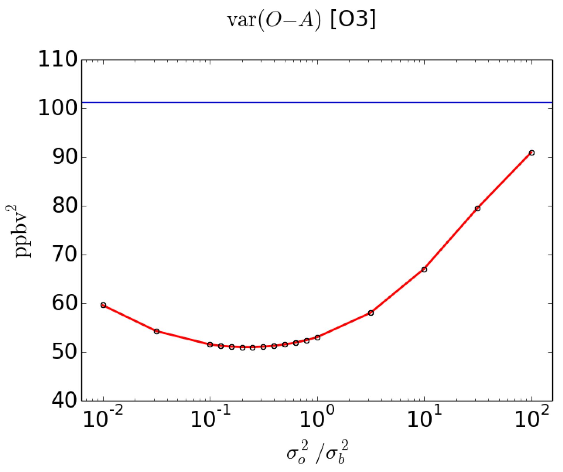
The red curve on Figure 2 illustrates how this diagnostic varies with and exhibits a minimum. This minimum can easily be understood by referring to Figure 1: as the analysis point changes position along the line the distance reaches a minimum, and this is what we observe in Figure 2.
In our next step, iter 1, we first re-estimate the correlation length by applying a maximum likelihood method, as in Ménard [15], using the iter 0 error variances that are consistent with the optimal ratio obtained in iter 0 and the innovation variance consistency. Then, with this new correlation length, we estimate a new optimal ratio (iter 1), which turn out to be very close to the value obtained in iter 0. We recall that we use uniform error variances, both to keep things simple but also because the optimal ratio is obtained by minimizing a domain-averaged variance . A summary of the error covariance parameters obtained for iter 0 and iter 1 are presented in Table 1.
We have also added in Table 1, the diagnostic values [15] which is the 60-day mean value of where is the total number of observations available at time and . The diagnostics [15] is closely related to the diagnostic used in variational methods, and should have a value of 1 in the case where the innovations are consistent with the prescribed error statistics. When there is innovation covariance consistency then but the reverse is not true. We observe that there was a significant improvement from iter 0 to iter 1 in terms of but is still not equal to one. We thus refer the analysis of iter 1 as near optimal.
The repeated application of this sequence of estimation methods, i.e., find the correlation length by maximum likelihood and optimize the variance ratio, converges really fast and in practice there is no need to go beyond iter 1. Figure 3 displays iterates 0 to 4 with our estimation procedure for O3. With one iteration update we nearly converge. A similar procedure was used in Ménard [15], where the variance and correlation length (estimated by maximum likelihood) were estimated in sequence, which taught us that a slow and fictitious drift in estimated variances and correlation length can occur when the correlation model is not the true correlation. So in regard of similar considerations that may occur here, we do not extend our iteration procedure beyond the first iterate.
3.2. Statistical Diagnostics of Analysis Error Variance
For each of these experiments, statistics related diagnostics for analysis error variance, discussed in Section 2, are computed and the results are presented in Table 2 for the verification made against active observations, and in Table 3 to the verification made against the passive observations. If the analysis was truly optimal the different diagnostics would all agree.
In the second, third and last column of Table 2 are tabulated estimates of the analysis error variance at the active location sites, i.e., , obtained by three different methods. The second column is an estimate given with our method . The third column is the Desroziers et al. estimate of analysis error [14], Equation (20), and the last column is the estimate using the method proposed by Hollingsworth and Lönnberg [13], Equation (18). We note that the analysis error variance estimate provided by the first two methods is fairly consistent for an updated correlation length estimate, i.e., iter 1 (but not iter 0). We also note that is closer to one for iter 1. These two facts indicate that the updated correlation length (iter 1) with uniform error variances is closer to the innovation covariance consistency. The Hollingsworth and Lönnberg [13] method however, is very sensitive and negatively biased in the lack of innovation covariance consistency.
Estimate of the analysis error variance at the passive observation locations, i.e., , provided by two different methods are given by Equation (21) in column 3 and by Equation (22) in column 5 of Table 3. As for the estimate at the active locations (Table 2), there is a general agreement on the analysis error estimates with the updated correlation length (iter 1), although this distinction is not that clear for PM2.5.
We note also that the analysis error variance at the active sites is smaller than the analysis error variance at the passive observation sites. This involves in particular the fact that since the passive observation are away from the active observation sites, the reduction of variance at the passive observation sites is smaller than at the active observation sites.
3.3. Comparison with the Perceived Analysis Error Variance
We computed the analysis error covariance resulting from the analysis scheme, the so-called perceived analysis covariance [6], using the expression,
Contrary to the statistical diagnostics above, the perceived analysis error variance is obtained at each model grid point. We then compared the perceived analysis error variance at the active observation sites with the estimated active analysis error variance obtained from previous diagnostics. Since we showed that in both active and passive observations sites the different diagnostics agrees when the analysis is optimal, this would indicate that if the perceived analysis error variance agrees with the analysis error variance diagnostics, that the whole map of analysis error variance is credible.
In order to calculate the perceived analysis error covariance Equation (23) we first perform a Choleski decomposition of , where is a lower triangular matrix. Then with a forward substitution we obtain , from which we compute . The perceived analysis error variance for the ozone optimal analysis (i.e., O3 iter 1) is displayed in Figure 4 (A similar figure but for PM2.5 is given in supplementary material). We note that although the input statistics used for the analysis are uniform (i.e., uniform background and observation error variances, and homogeneous correlation model), the computed analysis error variance at the active observation location displays large variations, which is attributed to the non-uniform spatial distribution of the active observations.
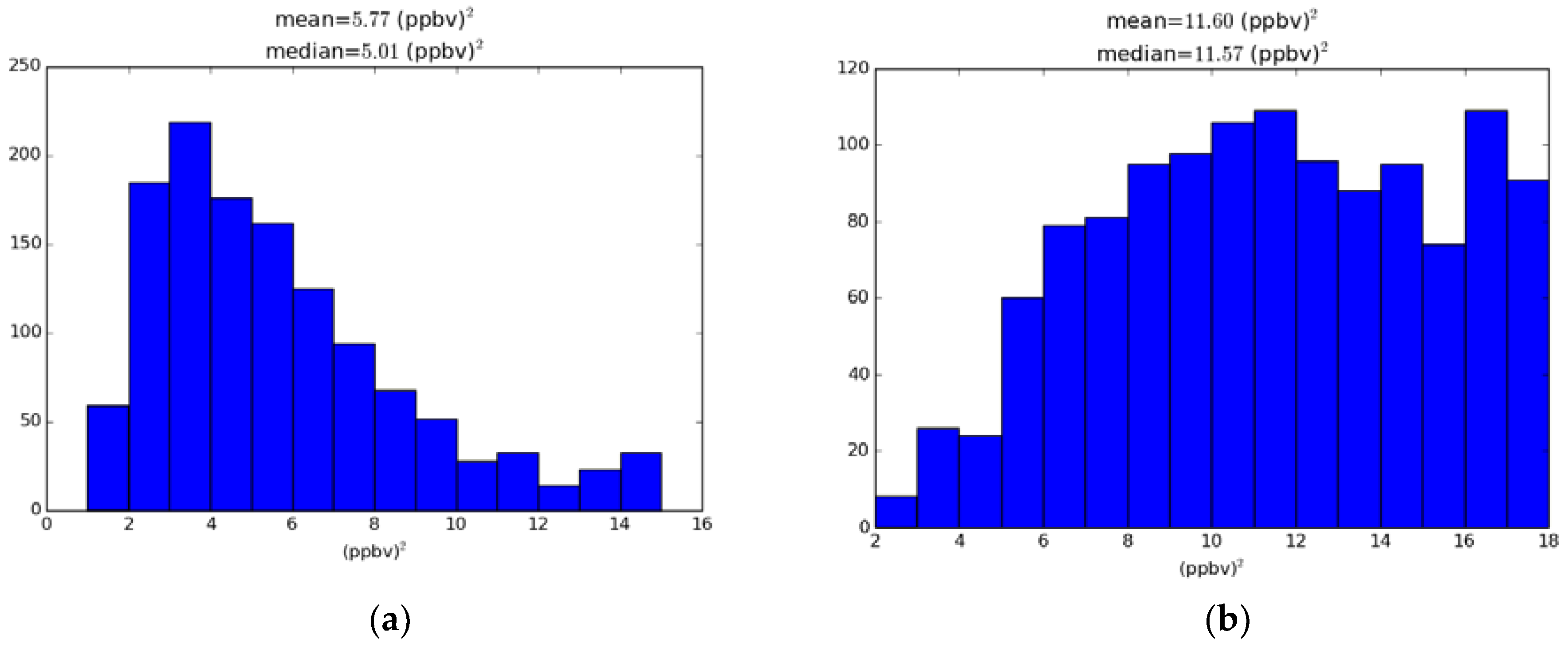
In Figure 5 we display a histogram of those variances for the ozone optimal analysis O3 iter 1 (panel b) and for the first experiment O3 iter 0 (panel a) without optimization (A similar figure is but for PM2.5 is given in supplementary material).
Note that median or mean values of variances are significantly different between the optimal and non-optimal analysis cases. Although the observation and background errors are uniform in both optimal and non-optimal analyses, in the optimal analysis case the perceived analysis uncertainty at the observation location is distributed more equally across all values, indicating that there is a better propagation of information, measured by analysis error variance, across the different observation sites. The exception being the isolated observation sites, for which we observe a maxima on the high end of the histograms. At those sites the analysis error variance is simply obtained by the scalar equation . For O3 iter 1 the scalar analysis error variance gives 16.2, and for O3 iter 0 we get 15.0, thus explaining the secondary maxima on the high end of the histogram.
The mean perceived analysis error variance for all experiments is presented in Table 4. Comparing these values with the estimated values of analysis error variance based on diagnostics in Table 2 we note that for both optimal experiments, O3 iter 1 and PM2.5 iter 1, the perceived analysis error variance roughly agrees with all analysis error variances estimated with diagnostics (Table 2).
However, for the non-optimal analyses, O3 iter 0 and PM2.5 iter 0, there is a general disagreement between all estimated values. Looking more closely, however, we note that the agreement in the optimal case is not perfect. The perceived analysis error variance is about 20% lower than the best estimates and . The optimal values in the “optimal” cases are slightly above one, thus indicating that the innovation covariance consistency is not exact and some further tuning of the error statistics could be done. More on that matter will be presented in Section 4.5.
4. Discussion on the Statistical Assumptions and Practical Applications
4.1. Representativeness Error with In situ Observations
The statistical diagnostics presented in Section 2 derive from the assumption that the observation errors are horizontally uncorrelated and uncorrelated with the background error. Although this assumption is never entirely observed in reality, there are ways to work around it. In the case of in situ observations, and assuming that any systematic error have been removed, random errors are still present, due to the difference between the observation and the model’s equivalent of the observation—called representativeness error (see Janjic et al. [12] for a review). Representativeness error is due to unresolved scales and processes in the model and interpolation or forward observation model errors. These errors are typically roughly at the scale of the model grid [21,22], so typically a few tens of kilometers for air quality models. This should not be confused with the representativeness of an observation, where, for example, remote stations are representative of large area (e.g., several hundreds of kilometers), whereas urban and suburban stations are at the scale of human activity in the cities, traffic and industries, etc. and are, depending on the chemical specie, of a few kilometers and less.
Representativeness error of in situ measurements can be discarded altogether by simply filtering any pair of observations that are in the range of a few model grid sizes, both in assimilation and estimation of error statistics [1] or in pairs of passive-active observations for cross-validation [17]. Once this filtering is done, the assumption on observation errors being spatially uncorrelated and uncorrelated with the background error then applies.
4.2. Correlated Observation-Background Errors
In any case, it is interesting to show how the different diagnostics, introduced in Section 2, depends on the statistical assumptions of the observation error. One way to get an understanding of the effect of these assumptions is to look at it from a geometrical point of view, using the representation introduced in Section 2.2. Note that the same results can be obtained analytically, but the geometrical interpretation gives a simple and appealing way of looking at the problem.
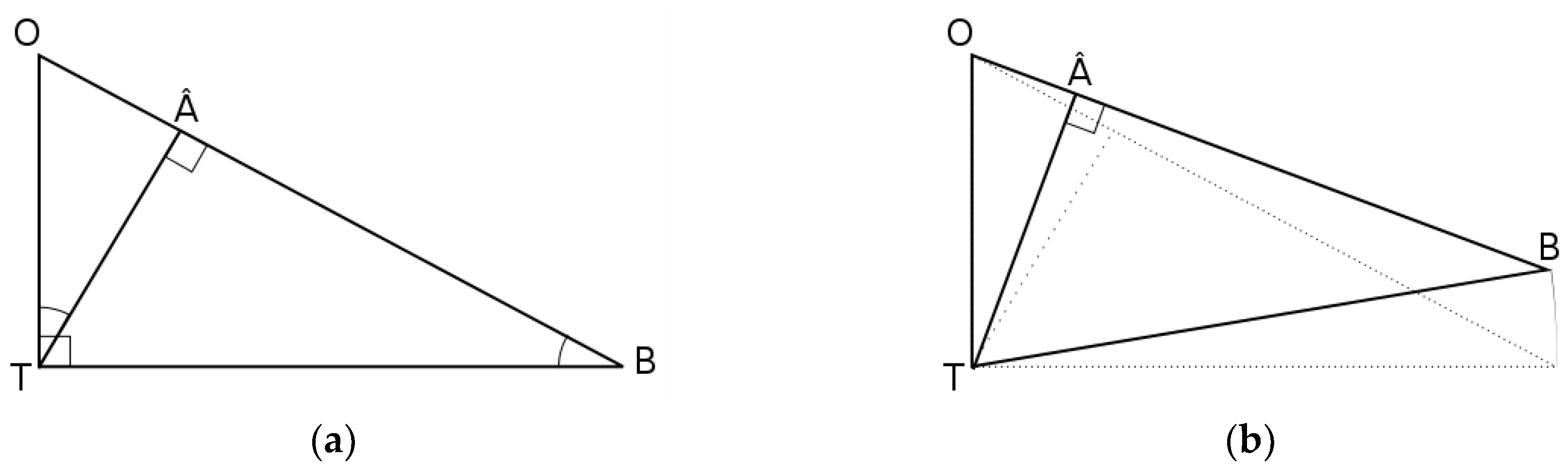
Let us consider the effect on the analysis of observation error correlated with background error. The case where the observation error is uncorrelated with background error is represented in Figure 6 on the panel a and when they are correlated on the panel b.
The observation and background error variances are kept unchanged, with the same length and length in both panels. In the case of correlated errors the angle is no longer a right angle. Yet, it is still possible to obtain an optimal analysis, , as a linear combination of the observation and the background, on the line , for which the distance to T (i.e., the analysis error variance) is minimum. In this case, . Note that for strongly correlated errors and when , although is still on the line , it may actually lie outside the segment . Yet, the principles and theory still hold in that case.
When the observation error is uncorrelated with the background error, , the triangles and are similar and it follows that , which is the Desroziers et al. [14] diagnostic for analysis error variance. However, when the observation error is correlated with the background error (right panel of Figure 6), the triangles and are no longer similar triangles and the Desroziers et al. [14] diagnostics for analysis error does not hold (see derivation in Appendix A). However, the HL, Equation (18), and MDJ diagnostic, Equation (19), depend only on having right triangles and , and not on the orthogonality of with . Therefore, the HL and MDJ diagnostics are valid with or without correlated observation-background errors.
4.3. Estimation of Satellite Observation Errors with In situ Observation Cross-Validation
One of the important problems in satellite assimilation is the estimation of the satellite observation error, which could be addressed with a simple modification of our cross-validation procedure. Let us assume that we have in situ observations that we assume to have uncorrelated errors between themselves (or use a filter with a minimum distance as discussed in Section 4.1), with the background errors and the satellite observation errors. Yet, the satellite observation errors could be correlated with the background error. Satellite observations could come from a multi-channel instrument with channel-correlated observation errors, as found with many instruments, and yet our validation procedure can still be used. Let us consider that the analyses comprise of satellite and in situ observations but, for the purpose of cross-validation, we use only 2/3rd of the in situ observations in the analysis, and keep the remaining 1/3rd as passive to carry out the cross-validation procedure.
The first thing to note is that the passive in situ observations have uncorrelated errors with the analysis error (the analysis is composed of satellite observations and 2/3rd of the in situ observations). We then use Equation (7) where the interpolation of the analysis is made only at the in situ active observations. Minimizing (i.e., the trace of the left hand side of Equation (7)) results in finding the optimal in situ observation weight. Then, computing the analysis error covariance in the satellite observation space from the analysis scheme (either from a Hessian of a variational cost function, or with an explicit gain as in Equation (23)), i.e., , we use the HL formulation Equation (18) to obtain the satellite observation error covariance,
The Equation (24) has the important properties that the estimated observation error covariance is symmetric and positive definite by construction. Then, a new analysis could be carried out to obtain a more realistic , with a resulting updated , and so forth until convergence.
4.4. Remark on Cross-Validation of Satellite Retrievals
As a last remark, it appears that cross-validation of satellite retrieval observations using a k-fold approach where the observations are used as passive observations to validate the analysis can be a difficult problem. Retrievals from passive remote sensing at nadir generally involve a prior or climatology or a model assumption over different regions, and is thus likely to have spatially correlated errors and errors correlated with the background error. It does not mean, however, that nothing can be done in that case. For example, for certain sensors, such as infrared sensors, it is possible to disentangle the prior from the retrieval, so that by an appropriate transformation of the measurements, observations can be practically decorrelated from the background [23,24]. However to the authors’ knowledge, such an approach have never been undertaken for visible measurements such as for NO2 or AOD’s.
4.5. Lack of Innovation Covariance Consistency and Its Relevance to the Statistical Diagnostics
The error covariance diagnostics for optimal analysis, presented in Section 2.4 and Section 2.5, depends on the innovation covariance consistency, , and our results presented in Section 3 have shown that the different estimates for the optimal analysis error variance are close, but do not strictly agree to each other. This disagreement is related to the lack of innovation consistency as follows.
Let us introduce a departure matrix from innovation covariance consistency as,
The trace of Equation (25), which is related to , is given by
We recall that in the experiment iter 1 we got values of 1.36 for O3 and 1.25 for PM2.5 (see Table 1), indicating that the innovation covariance consistency is deficient, although less serious than with the experiment iter 0 where values of 2 and higher have been obtained.
If we take into account the fact that there can be a difference between and and we rederive the (active) analysis error covariance for HL, MDJ and D schemes, we get (see Appendix B)
where , . We note that although the error terms are complex expressions, they all depend linearly on . Thus, the disagreement between the HL, MDJ and D analysis error variance estimates is due to lack of innovation covariance consistency.
5. Conclusions
We showed that analysis error variance can be estimated and optimized, without using a model forecast, by partitioning the original observation data set into a training set, to create the analysis, and an independent (or passive) set, used to evaluate the analysis. This kind of evaluation by partitioning is called cross-validation. The method derives from assuming that the observations have spatially uncorrelated errors or, minimally, that the independent (or passive) observations have uncorrelated errors with the active observation, and are uncorrelated the background error. This leads to the important property that passive observations are uncorrelated with the analysis error and can then be used to evaluate the analysis [17].
We have developed a theoretical framework and a geometric interpretation that has allowed us to derive a number of statistical estimation formulas of analysis error covariance that can be used in both passive and active observation spaces. It is shown that by minimizing the variance of observation-minus-analysis residuals in passive observation space we actually identify the optimal analysis. This has been done with respect to a single parameter, namely the ratio of observation to background error variances, to obtain a near optimal Kalman gain. The optimization is also done under the constraint of the innovation covariance consistency [14,15]. This optimization could have been done with more than one error covariance parameter but this has not been attempted here. The theory does suggest, however, that the minimum is unique.
Once an optimal analysis is identified we conduct an evaluation of the analysis error covariance using several different formulas; Desroziers et al. [14], Hollingsworth Lönnberg [13], and one that we develop in this paper which works in either active or passive observation spaces. As a way to validate the analysis error variance computed by the analysis scheme itself, the so-called perceived analysis error variance [6], we compare it with the values obtained from the different statistical diagnostics of analysis error variance.
This methodology arises from a need to assess and improve ECCC’s surface air quality analyses using our operational air quality model GEM-MACH and real-time surface observations of O3 and PM2.5. Our method applied the theory in a simplified way. First by considering the averaged observation and background error variances and finding an optimal ratio using as a constraint the trace of the innovation covariance consistency [15]. Second, using a single parameter correlation model, its correlation length, we used the maximum likelihood estimation [11] to obtain near optimal analyses. Also we did not attempt to account for representativeness error in the observations by, for example, filtering observations that are close. Despite all these limitations, our results show that with near optimal analyses, all estimates of analysis error variance roughly agree with each other, while disagreeing strongly when the input error statistics are not optimal. This check on estimating the analysis error variance gives us confidence that the method we propose is reliable, and provides us an objective method to evaluate different analysis components configurations, such as the type of background error correlation model, the spatial distribution of error variances and possibly the use of thinning observations to circumvent effects of representativeness errors.
The methodology introduced here for estimating analysis error variances is general and not restricted to the case of surface pollutant analysis. It would be desirable to investigate other areas of applications, such as surface analysis in meteorology and oceanography. The method could, in principle, provide guidance for any assimilation system. By considering the observation space subdomain [25], proper scaling, local averaging [26], or other methods discussed in Janjic et al. [12] it may also be possible to extend this methodology to spatially varying error statistics. Based on our verification results in Part I [5], we found that there is a dependence between model values and error variances, which we will investigate further in view of our next operational implementation of the Canadian surface air quality analysis and assimilation.
One strong limitation of the optimum interpolation scheme we are using (i.e., homogeneous isotropic error correlation and uniform error variances), which is also the case for most 3D-Var implementations, is the lack of innovation covariance consistency. Ensemble Kalman filters seem, however, much better in that regard although they have their own issues with localization and inflation. Experiments with chemical data assimilation using an ensemble Kalman filter does gives values very close to unity after simple adjustments for observation and model error variances [27]. We thus argue that ensemble methods, such as the ensemble Kalman filter, would produce analysis error variance estimates that are much more consistent between the different diagnostics.
Estimates of analysis uncertainties can also be obtained by resampling techniques, such as the jackknife method and bootstrapping [28]. In bootstrapping with replacement, the distribution of the analysis error is obtained by creating new analyses by replacing and duplicating observations from an existing set of observations [28]. This technique relies on the assumption that each member of the dataset is independent and identically distributed. For surface ozone analyses where there is persistence to next day and the statistics is spatially inhomogeneous, the assumption of statistical independence may not be adequate. The comparison of these resampling estimates of analysis uncertainties could be compared with our analysis error variance estimates to help us identify limitations and areas of improvement.
Supplementary Materials
The following are available online at https://www.mdpi.com/2073-4433/9/2/70/s1, Figure S1: Analysis error variance for ozone optimal analysis case PM2.5 iter 1. Left panel is the analysis error on the model grid and on the right panel at the active observation sites. Note that the color bar of the left and right panels are different. The maximum of the color bar for the left panel correspond to , Figure S2: Distribution (histogram) of the ozone analysis error variance at the active observation locations. First analysis experiment PM2.5 iter 0 (no optimization) on the left panel, and optimal analysis case PM2.5 iter 1 on the right panel.
Acknowledgments
We are grateful to the US/EPA for the use of the AIRNow database for surface pollutants and to all provincial governments and territories of Canada for kindly transmitting their data to the Canadian Meteorological Centre to produce the surface analysis of atmospheric pollutants. We are also thankful for the proof read by Kerill Semeniuk, and for two anonymous reviewers for their comments and help in improving the manuscript.
Author Contributions
This research was conducted as a joint effort by both authors. R.M. contributed to the theoretical development and wrote the paper, and M.D.-J. conducted all experiments design and execution, proof reading and introduced a new diagnostic of optimal analysis error that was further extended to passive observations space.
Conflicts of Interest
The authors declare no conflict of interest. The founding sponsors, which is the government of Canada, had no role in the design of the study; in the collection, analyses, or interpretation of data; in the writing of the manuscript, and in the decision to publish the results.
Appendix A. A Geometrical Derivation of the Desroziers et al. Diagnostic
Let and be two random variables of a real Hilbert space as defined in Section 2.3. Two properties of Hilbert spaces are: the polarization identity
and the parallelogram identity [19]
Combining these two equations, we get:
Let and , then , and so we have
If we assume that the analysis is optimal, so that is a right triangle (see Figure 1), then
and similarly that is a right triangle,
and substitute these expression into Equation (A4) we get
If in addition we assume that we have uncorrelated observation-background errors, that is
we then get
Note that the difference with the result obtained in Appendix A (property 6) of Ménard [15] where it is shown that the necessary and sufficient condition for the perceived analysis error covariance in active observation space to meet the Desroziers et al. diagnostics for analysis error, is to have innovation covariance consistency and uncorrelated observation-background errors. The result obtained here is different; it concerns the optimal analysis error covariance.
Appendix B. Diagnostics of Analysis error Covariance and the Innovation Covariance Consistency
Let us introduce a departure matrix from innovation covariance consistency as,
The HL diagnostic, Equation (18), can be expanded as
where the is given as
which includes three error terms. A scalar version of Equation (A11) is given as
The error analysis for the MDJ diagnostic, Equation (19) is
where the is given as
There is only one term, and its scalar version is given as,
The error analysis for the Desroziers et al. diagnostic, Equation (20) is
where the is given as
Again only one error term that is similar to the MDJ diagnostic, and its scalar version is given as,
Error analysis for the diagnostics using passive observations can also be derived. For the passive MDJ diagnostics, Equation (21), we have similarly to (A14),
with a single error term given as,
To express a scalar version of this equation we need to account for the background error correlation between the active observation location and the passive observation location, and thus expressed as,
Finally, the fundamental diagnostic of cross-validation Equation (7) does not depend explicitly on the innovation covariance consistency. However, attaining its true minimum by tuning only and as would suggest Equation (22), does introduce some innovation in-consistency, which all other optimal diagnostics Equations (18)–(21) has to account for.
References
- Ménard, R.; Robichaud, A. The chemistry-forecast system at the Meteorological Service of Canada. In Proceedings of the ECMWF Seminar Proceedings on Global Earth-System Monitoring, Reading, UK, 5–9 September 2005; pp. 297–308. [Google Scholar]
- Robichaud, A.; Ménard, R. Multi-year objective analysis of warm season ground-level ozone and PM2.5 over North-America using real-time observations and Canadian operational air quality models. Atmos. Chem. Phys. 2014, 14, 1769–1800. [Google Scholar] [CrossRef]
- Robichaud, A.; Ménard, R.; Zaïtseva, Y.; Anselmo, D. Multi-pollutant surface objective analyses and mapping of air quality health index over North America. Air Qual. Atmos. Health 2016, 9, 743–759. [Google Scholar] [CrossRef] [PubMed]
- Moran, M.D.; Ménard, S.; Pavlovic, R.; Anselmo, D.; Antonopoulus, S.; Robichaud, A.; Gravel, S.; Makar, P.A.; Gong, W.; Stroud, C.; et al. Recent advances in Canada’s national operational air quality forecasting system. In Proceedings of the 32nd NATO-SPS ITM, Utrecht, The Netherlands, 7–11 May 2012. [Google Scholar]
- Ménard, R.; Deshaies-Jacques, M. Evaluation of analysis by cross-validation. Part I: Using verification metrics. Atmosphere 2018, in press. [Google Scholar]
- Daley, R. The lagged-innovation covariance: A performance diagnostic for atmospheric data assimilation. Mon. Weather Rev. 1992, 120, 178–196. [Google Scholar] [CrossRef]
- Daley, R. Atmospheric Data Analysis; Cambridge University Press: New York, NY, USA, 1991; p. 457. [Google Scholar]
- Talagrand, O. A posteriori evaluation and verification of analysis and assimilation algorithms. In Proceedings of Workshop on Diagnosis of Data Assimilation Systems, November 1998; European Centre for Medium-Range Weather Forecasts: Reading, UK, 1999; pp. 17–28. [Google Scholar]
- Todling, R. Notes and Correspondence: A complementary note to “A lag-1 smoother approach to system-error estimaton”: The intrinsic limitations of residuals diagnostics. Q. J. R. Meteorol. Soc. 2015, 141, 2917–2922. [Google Scholar] [CrossRef]
- Hollingsworth, A.; Lönnberg, P. The statistical structure of short-range forecast errors as determined from radiosonde data. Part I: The wind field. Tellus 1986, 38A, 111–136. [Google Scholar] [CrossRef]
- Ménard, R.; Deshaies-Jacques, M.; Gasset, N. A comparison of correlation-length estimation methods for the objective analysis of surface pollutants at Environment and Climate Change Canada. J. Air Waste Manag. Assoc. 2016, 66, 874–895. [Google Scholar] [CrossRef] [PubMed]
- Janjic, T.; Bormann, N.; Bocquet, M.; Carton, J.A.; Cohn, S.E.; Dance, S.L.; Losa, S.N.; Nichols, N.K.; Potthast, R.; Waller, J.A.; et al. On the representation error in data assimilation. Q. J. R. Meteorol. Soc. 2017. [Google Scholar] [CrossRef]
- Hollingsworth, A.; Lönnberg, P. The verification of objective analyses: Diagnostics of analysis system performance. Meteorol. Atmos. Phys. 1989, 40, 3–27. [Google Scholar] [CrossRef]
- Desroziers, G.; Berre, L.; Chapnik, B.; Poli, P. Diagnosis of observation-, background-, and analysis-error statistics in observation space. Q. J. R. Meteorol. Soc. 2005, 131, 3385–3396. [Google Scholar] [CrossRef]
- Ménard, R. Error covariance estimation methods based on analysis residuals: Theoretical foundation and convergence properties derived from simplified observation networks. Q. J. R. Meteorol. Soc. 2016, 142, 257–273. [Google Scholar] [CrossRef]
- Kailath, T. An innovation approach to least-squares estimation. Part I: Linear filtering in additive white noise. IEEE Trans. Autom. Control 1968, 13, 646–655. [Google Scholar]
- Marseille, G.-J.; Barkmeijer, J.; de Haan, S.; Verkley, W. Assessment and tuning of data assimilation systems using passive observations. Q. J. R. Meteorol. Soc. 2016, 142, 3001–3014. [Google Scholar] [CrossRef]
- Waller, J.A.; Dance, S.L.; Nichols, N.K. Theoretical insight into diagnosing observation error correlations using observation-minus-background and observation-minus-analysis statistics. Q. J. R. Meteorol. Soc. 2016, 142, 418–431. [Google Scholar] [CrossRef]
- Caines, P.E. Linear Stochastic Systems; John Wiley and Sons: New York, NY, USA, 1988; p. 874. [Google Scholar]
- Cohn, S.E. The principle of energetic consistency in data assimilation. In Data Assimilation; Lahoz, W., Boris, K., Richard, M., Eds.; Springer: Berlin/Heidelberg, Germany, 2010. [Google Scholar]
- Mitchell, H.L.; Daley, R. Discretization error and signal/error correlation in atmospheric data assimilation: (I). All scales resolved. Tellus 1997, 49A, 32–53. [Google Scholar] [CrossRef]
- Mitchell, H.L.; Daley, R. Discretization error and signal/error correlation in atmospheric data assimilation: (II). The effect of unresolved scales. Tellus 1997, 49A, 54–73. [Google Scholar] [CrossRef]
- Joiner, J.; da Silva, A. Efficient methods to assimilate remotely sensed data based on information content. Q. J. R. Meteorol. Soc. 1998, 124, 1669–1694. [Google Scholar] [CrossRef]
- Migliorini, S. On the quivalence between radiance and retrieval assimilation. Mon. Weather Rev. 2012, 140, 258–265. [Google Scholar] [CrossRef]
- Chapnik, B.; Desroziers, G.; Rabier, F.; Talagrand, O. Properties and first application of an error-statistics tunning method in variational assimilation. Q. J. R. Meteorol. Soc. 2005, 130, 2253–2275. [Google Scholar] [CrossRef]
- Ménard, R.; Deshiaes-Jacques, M. Error covariance estimation methods based on analysis residuals and its application to air quality surface observation networks. In Air Pollution and Its Application XXV; Mensink, C., Kallos, G., Eds.; Springer International AG: Cham, Switzerland, 2017. [Google Scholar]
- Skachko, S.; Errera, Q.; Ménard, R.; Christophe, Y.; Chabrillat, S. Comparison of the ensemlbe Kalman filter and 4D-Var assimilation methods using a stratospheric tracer transport model. Geosci. Model Dev. 2014, 7, 1451–1465. [Google Scholar] [CrossRef]
- Efron, B. An Introduction to Boostrap; Chapman & Hall: New York, NY, USA, 1993; p. 436. [Google Scholar]
Figure 1.
Hilbert space representation of a scalar analysis and cross-validation problem. The arrows indicate the directions of variability of the random variables, and the plane defined by the background and observation errors , defines the analysis plane. The thick lines represent the norm associated with the different random variables. T indicate the truth, O the active observation, B the background, A the analysis and Oc the passive observation.
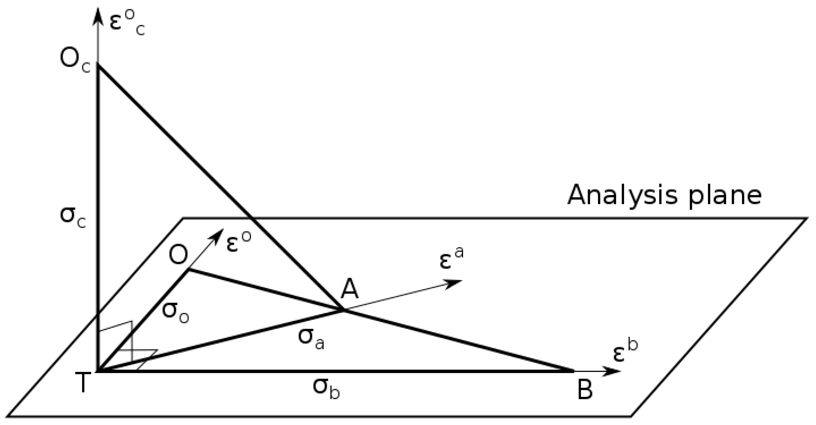
Figure 2.
Red line, variance of observation-minus-analysis of O3 in passive observation space. Blue line, variance of observation-minus-model.
Figure 2.
Red line, variance of observation-minus-analysis of O3 in passive observation space. Blue line, variance of observation-minus-model.

Figure 3.
Optimal estimates of , and maximum likelihood estimate of correlation length for the first four iterates. Blue, is the optimal background error variance, green, the optimal observation error variance and in red the correlation length (in km, with labels on the right side of the figure).
Figure 3.
Optimal estimates of , and maximum likelihood estimate of correlation length for the first four iterates. Blue, is the optimal background error variance, green, the optimal observation error variance and in red the correlation length (in km, with labels on the right side of the figure).
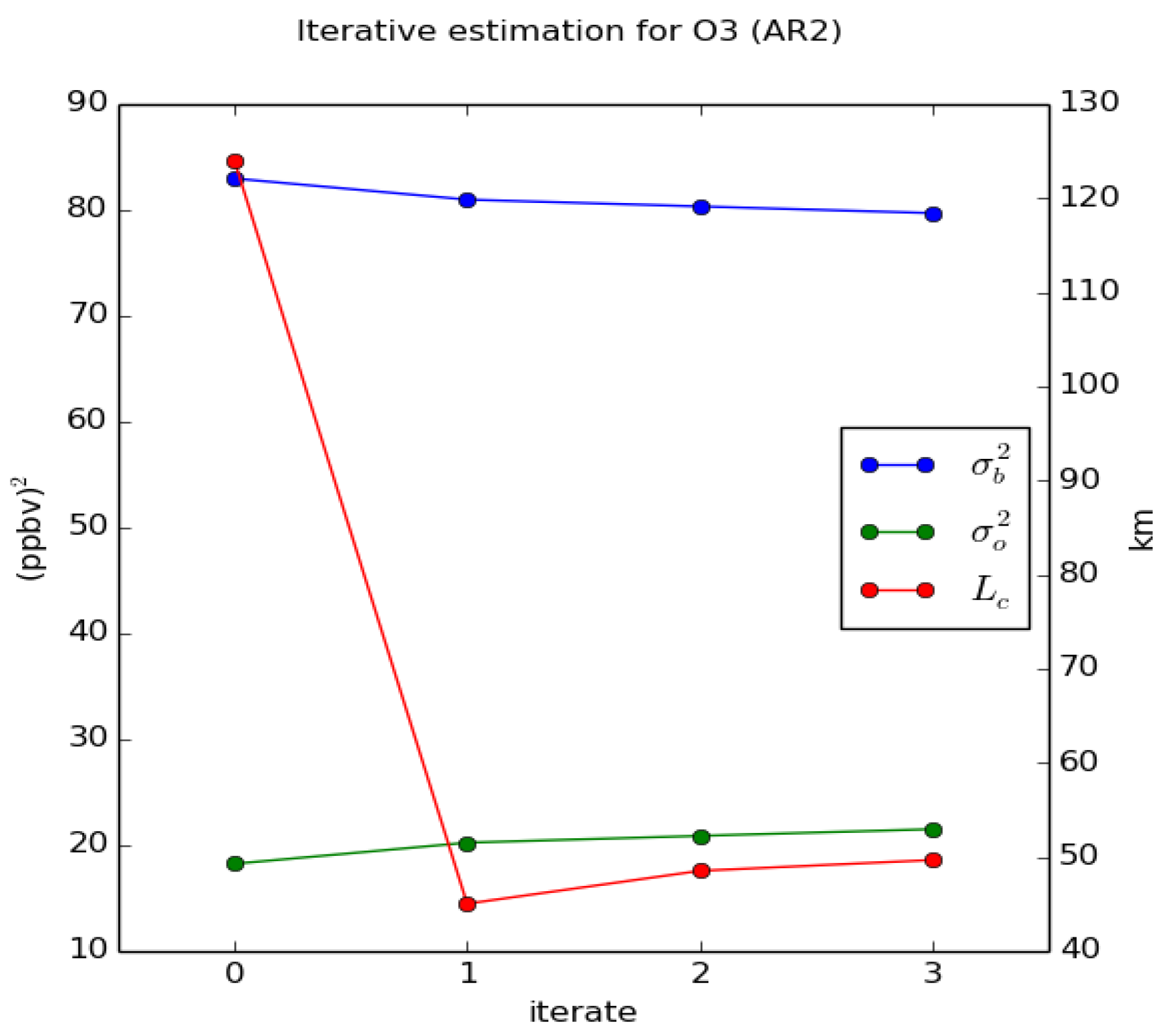
Figure 4.
Analysis error variance for ozone optimal analysis case O3 iter 1. (a) is the analysis error on the model grid and (b) at the active observation sites. Note that the color bar of the left and right panels are different. The maximum of the color bar for the left panel correspond to .
Figure 4.
Analysis error variance for ozone optimal analysis case O3 iter 1. (a) is the analysis error on the model grid and (b) at the active observation sites. Note that the color bar of the left and right panels are different. The maximum of the color bar for the left panel correspond to .
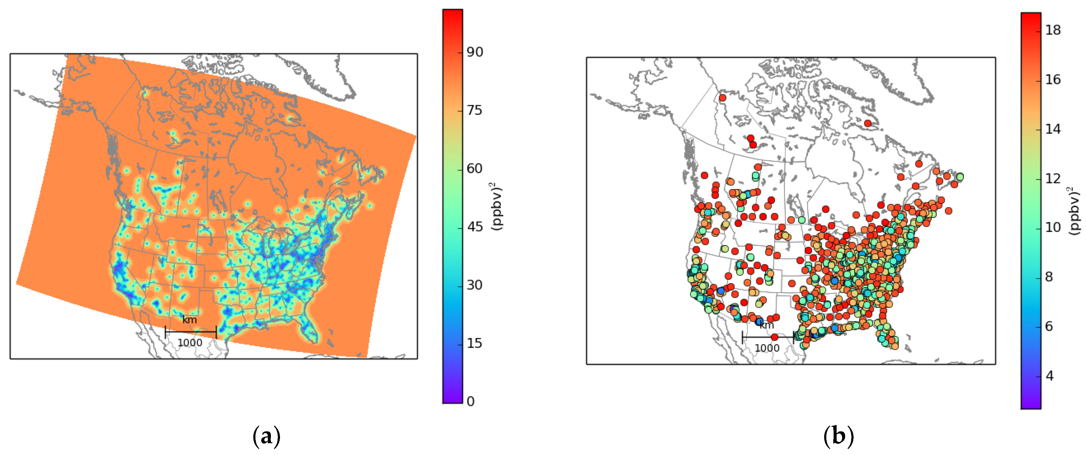
Figure 5.
Distribution (histogram) of the ozone analysis error variance at the active observation locations. (a) First analysis experiment O3 iter 0 (no optimization) on the left panel; (b) Optimal analysis case O3 iter 1. Note that the scales are different between the left and right panels.
Figure 5.
Distribution (histogram) of the ozone analysis error variance at the active observation locations. (a) First analysis experiment O3 iter 0 (no optimization) on the left panel; (b) Optimal analysis case O3 iter 1. Note that the scales are different between the left and right panels.

Figure 6.
Geometrical representation of the analysis. (a) for observation errors uncorrelated with the background error. (b) with correlated errors. T indicate the truth, O the observation, B the background and the optimal analysis.
Figure 6.
Geometrical representation of the analysis. (a) for observation errors uncorrelated with the background error. (b) with correlated errors. T indicate the truth, O the observation, B the background and the optimal analysis.

Table 1.
Input error statistics for the first experiment and optimized variance ratio experiment.
| Experiment | (km) | |||||
| O3 iter 0 | 124 | 101.25 | 0.22 | 18.3 | 83 | 2.23 |
| O3 iter 1 | 45 | 101.25 | 0.25 | 20.2 | 81 | 1.36 |
| PM2.5 iter 0 | 196 | 93.93 | 0.17 | 13.6 | 80.3 | 2.04 |
| PM2.5 iter 1 | 86 | 93.93 | 0.22 | 16.9 | 77 | 1.25 |
Table 2.
Analysis statistics against active observations.
| Experiment | Active | Active | Active | Active | Active |
| O3 iter 0 | 60.29 | 22.69 | 9.61 | 24.33 | −6.03 |
| O3 iter 1 | 67.66 | 13.32 | 13.68 | 11.26 | 8.94 |
| PM2.5 iter 0 | 62.29 | 17.98 | 7.71 | 16.78 | −3.18 |
| PM2.5 iter 1 | 66.3 | 10.68 | 9.51 | 9.57 | 7.33 |
Table 3.
Analysis statistics against passive observations.
| Experiment | Passive | Passive | Passive | Passive |
| O3 iter 0 | 56.95 | 26.03 | 51.02 | 32.72 |
| O3 iter 1 | 52.04 | 28.95 | 48.95 | 28.75 |
| PM2.5 iter 0 | 62.29 | 22.65 | 38.09 | 24.49 |
| PM2.5 iter 1 | 66.3 | 24.62 | 38.28 | 21.38 |
Table 4.
Perceived analysis error variance. Mean over active observation sites.
| Experiment | Perceived |
| O3 iter 0 | 5.77 |
| O3 iter 1 | 11.60 |
| PM2.5 iter 0 | 4.37 |
| PM2.5 iter 1 | 8.21 |
© 2018 by the authors. Licensee MDPI, Basel, Switzerland. This article is an open access article distributed under the terms and conditions of the Creative Commons Attribution (CC BY) license (http://creativecommons.org/licenses/by/4.0/).
Share and Cite
MDPI and ACS Style
Ménard, R.; Deshaies-Jacques, M. Evaluation of Analysis by Cross-Validation, Part II: Diagnostic and Optimization of Analysis Error Covariance. Atmosphere 2018, 9, 70. https://doi.org/10.3390/atmos9020070
AMA Style
Ménard R, Deshaies-Jacques M. Evaluation of Analysis by Cross-Validation, Part II: Diagnostic and Optimization of Analysis Error Covariance. Atmosphere. 2018; 9(2):70. https://doi.org/10.3390/atmos9020070
Chicago/Turabian StyleMénard, Richard, and Martin Deshaies-Jacques. 2018. "Evaluation of Analysis by Cross-Validation, Part II: Diagnostic and Optimization of Analysis Error Covariance" Atmosphere 9, no. 2: 70. https://doi.org/10.3390/atmos9020070
Note that from the first issue of 2016, this journal uses article numbers instead of page numbers. See further details here.