Evaluations of WRF Sensitivities in Surface Simulations with an Ensemble Prediction System

National Center for Atmospheric Research, Boulder, CO 80301, USA
*
Author to whom correspondence should be addressed.
Atmosphere 2018, 9(3), 106; https://doi.org/10.3390/atmos9030106
Submission received: 26 January 2018
/
Revised: 9 March 2018
/
Accepted: 9 March 2018
/
Published: 13 March 2018
(This article belongs to the Special Issue WRF Simulations at the Mesoscale: From the Microscale to Macroscale)
Abstract
:This paper investigates the sensitivities of the Weather Research and Forecasting (WRF) model simulations to different parameterization schemes (atmospheric boundary layer, microphysics, cumulus, longwave and shortwave radiations and other model configuration parameters) on a domain centered over the inter-mountain western United States (U.S.). Sensitivities are evaluated through a multi-model, multi-physics and multi-perturbation operational ensemble system based on the real-time four-dimensional data assimilation (RTFDDA) forecasting scheme, which was developed at the National Center for Atmospheric Research (NCAR) in the United States. The modeling system has three nested domains with horizontal grid intervals of 30 km, 10 km and 3.3 km. Each member of the ensemble system is treated as one of 48 sensitivity experiments. Validation with station observations is done with simulations on a 3.3-km domain from a cold period (January) and a warm period (July). Analyses and forecasts were run every 6 h during one week in each period. Performance metrics, calculated station-by-station and as a grid-wide average, are the bias, root mean square error (RMSE), mean absolute error (MAE), normalized standard deviation and the correlation between the observation and model. Across all members, the 2-m temperature has domain-average biases of −1.5–0.8 K; the 2-m specific humidity has biases from −0.5–−0.05 g/kg; and the 10-m wind speed and wind direction have biases from 0.2–1.18 m/s and −0.5–4 degrees, respectively. Surface temperature is most sensitive to the microphysics and atmospheric boundary layer schemes, which can also produce significant differences in surface wind speed and direction. All examined variables are sensitive to data assimilation.
1. Introduction
Mesoscale numerical weather prediction (NWP) models provide very valuable weather forecast guidance for lead times of hours to days. The Weather Research and Forecasting (WRF) model is a state-of-the-art mesoscale NWP modeling system designed for both atmospheric research and operational forecasting [1]. The WRF model offers operational forecasting as a flexible and computationally-efficient platform, while incorporating recent advances in physics, numerics and data assimilation contributed by developers from the expansive research community. The WRF model is currently in operational use at the United States (U.S.) at National Centers for Environmental Prediction (NCEP) and other national meteorological centers, as well as in real-time forecasting configurations at laboratories, universities and private companies. The WRF model has a large worldwide community of registered users because it is open source and runs on many computing platforms.
The number of physics options in the WRF model is simultaneously a strength and a challenge. As of Version 3.8.1, there are 17 schemes for microphysics, 13 for the atmospheric boundary layer (ABL), 14 for cumulus convection, 3 for shallow convection, 8 for shortwave radiation, 6 for longwave radiation, 8 for the surface layer and 9 for the land surface. Many studies show that surface variables can be sensitive to ABL physics [2,3,4,5,6,7,8,9,10], which impacts surface wind and wind energy resource simulations [11,12,13,14]. Precipitation forecasts and simulations of severe weather can be sensitive to cloud microphysics and cumulus parameterizations [15,16,17,18,19,20,21,22,23]. Surface variables (e.g., wind) can also be sensitive to the land surface model, land use and topography [24,25,26,27,28]. Data assimilation has an impact on atmospheric or oceanic models in general, and it also plays an important role in WRF model simulations [29]; post-processing can also improve the results [30]. However, further studies of the sensitivities of the different schemes, particularly those that are newly implemented, are needed. The system used in this study is an operational system developed for weather forecast for the Western United States. The system is mainly designed for surface high-resolution weather forecasts. The motivation of the sensitivity study is to choose better parameters for the modeling system. The Western United States has complex mountain areas, so that it is a big challenge for weather forecasting. This study will provide useful information for parameter setting for WRF simulation in the complex terrain area similar to the western United States of America (USA). The sensitivity of surface variables to the ABL scheme, cumulus parameterization, microphysics and boundary/initial condition will be investigated.
In this study, 48 experiments were conducted with an ensemble prediction system (EPS) [30]. Each member of the ensemble is treated as a different experiment to investigate model sensitivities to different configurations. The paper is organized as follows: model configurations, the experimental design and observation data sources used for verification are given in Section 2, followed by the evaluation of the sensitivities and additional comments in Section 3. Section 4 summaries the main results.
2. Model Setting, Experiments’ Design and Observation Data Sources
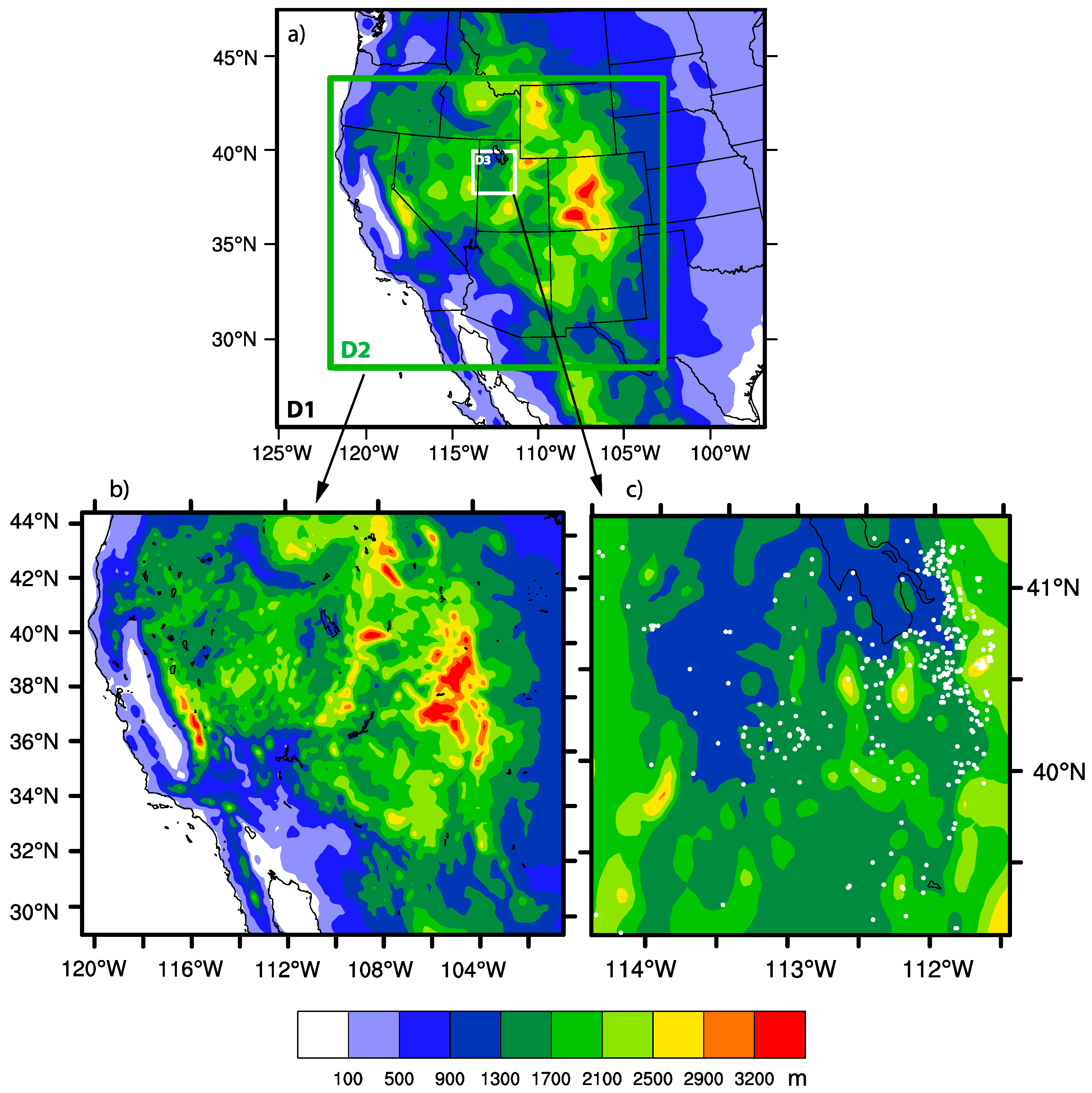
The study area focuses on the complex topography and high mountain ranges (e.g., Rocky Mountains and the Sierra Nevada) of the western United States. The modeling system has three domains (Figure 1a), with horizontal grid intervals of 30 km (98 × 84 points), 10 km (196 × 172) and 3.3 km (76 × 76). The model has 37 vertical levels. The advanced research WRF (ARW) Version 3.8.1 is used in this study. The WRF model integrates the fully-compressible non-hydrostatic equations of motion and can be run at cloud-resolving scale (e.g., around 3 km). In its standard configuration, it uses fifth order upwind advection and third order Runge–Kutta split explicit time integration [31]; it has low dispersion errors, and it allows a time step that is longer than in some other mesoscale models [32,33]. The experiments are listed in Table 1. Our two control configurations of the model use the Kain–Fritsch cumulus scheme [34], Lin microphysics [35], rapid radiative transfer model (RRTM) longwave radiation [36], Dudhia shortwave radiation [37], Yonsei University (YSU) ABL [38] and the Noah land-surface model [39]. One control configuration uses the Global Forecast System (GFS) as the boundary and initial condition, and the other control configuration uses the North American Mesoscale Forecast System (NAM) as the boundary and initial conditions. Then, different ABL, radiation, microphysics and cumulus parameterizations are tested, totaling 48 experiments (Table 1). For detailed descriptions of these schemes, please refer to the WRF model user’s guide [40] and web site (http://www2.mmm.ucar.edu/wrf/users/).
Each cycle is run every 6 h from 1200 UTC, 18 January 2016, through 1800 UTC, 26 January 2016 (the first period of study), and then, from 1200 UTC, 1 July 2016, through 1800 UTC, 9 July 2016 (the second period of study). The first 12 h at the start of each of the one-week periods is discarded to remove spin-up effects. Each cycle comprises a six-hour analysis (with data assimilation) and a 24-h forecast (without data assimilation). The first cycle gets the initial condition from the large-scale model (e.g., NAM or GFS), and the following cycle gets the initial condition from the restart file from the previous cycle. The results are verified by World Meteorological Organization (WMO) and NCEP Meteorological Assimilation Data Ingest System (MADIS) station observations [29]. Locations of the 344 surface stations in Domain 3 are given in Figure 1c.
3. Evaluation of the Sensitivities of the System
The sensitivity of the model to each configuration is assessed through domain average bias (observation mean subtracted from forecast mean), mean absolute error (MAE), root mean square error (RMSE), normalized standard deviation (forecast’s standard deviation/observation’s standard deviation) (Std) and the correlation (Cor) between forecasts and observations. The model outputs are linear interpolated to the observation point and height adjustment for temperature with empirical lapse rate (6.5 K/km).
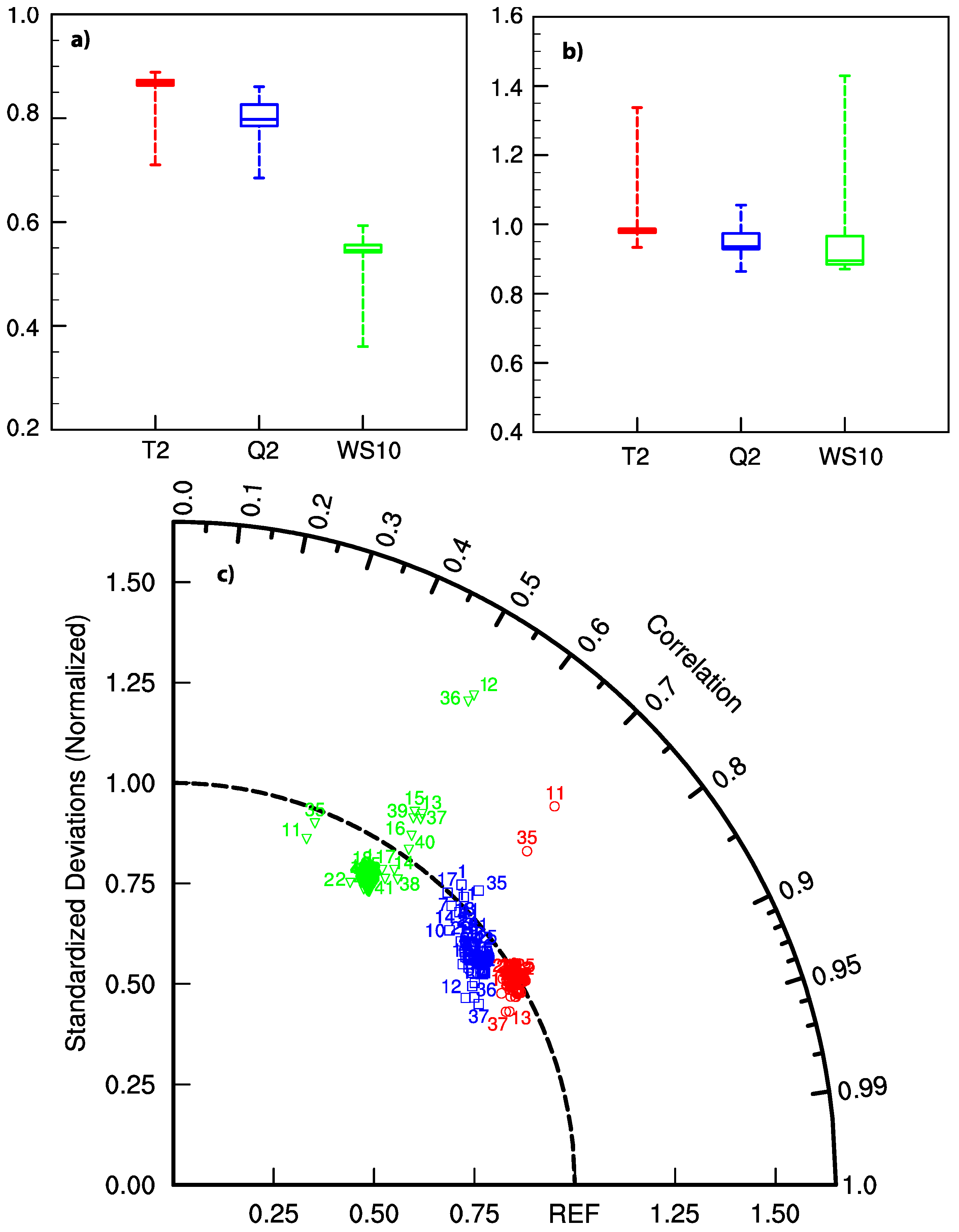
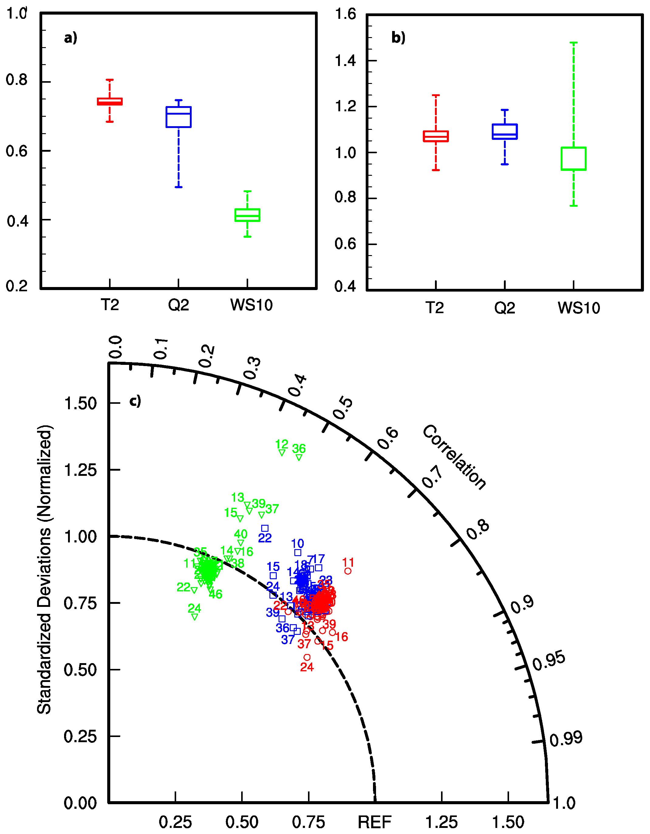
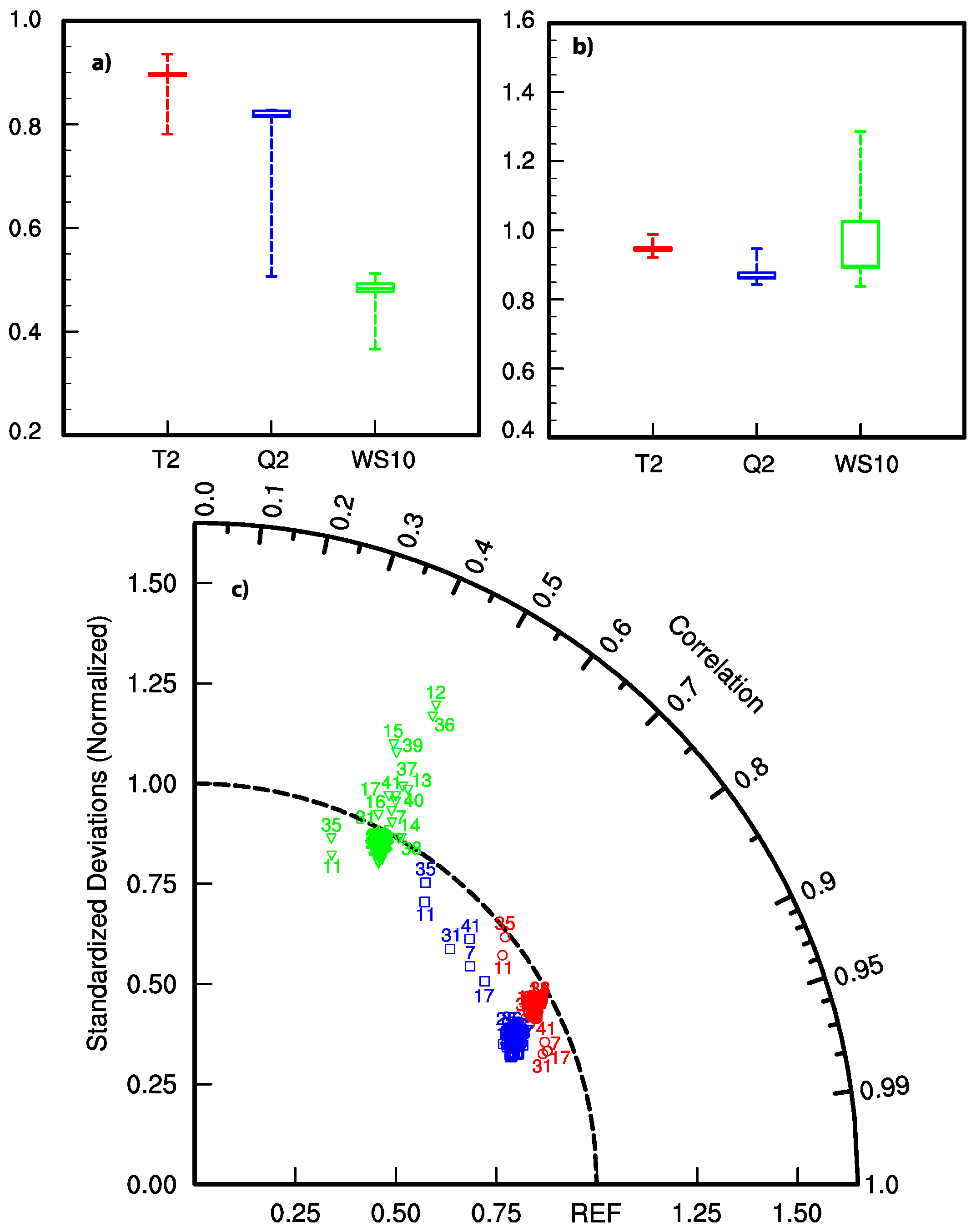
The results for normalized standard deviation and correlation between analyses/forecasts and observations are given in Figure 2, Figure 3, Figure 4 and Figure 5. Figure 2 presents the normalized standard deviation and correlation in analyses from the one-week period in January. Correlations between analyses and observations are around 0.87 for air temperature at 2 m above ground level (AGL) (T2), 0.8 for specific humidity at 2 m AGL (Q2) and 0.5 for wind speed at 10 m AGL (WS10) (Figure 2). The lower correlation in WS10 is caused by the variability in the wind field. The lowest correlations are from the experiments without data assimilation (11 GNODA, 35 NNODA), which also have some of the highest normalized standard deviations. Some ABL scheme experiments (12 GPBOU and 36 NPBOU) have even higher normalized standard deviations in WS10 (Figure 2). Generally, normalized standard deviations in WS10 are high and substantially above 1.0, among the experiments with ABL schemes (13 GPMYJ, 15 GPQNS, 37 NPMYJ and 39 NPQNS), different from the control scheme of YSU. Thus, WS10 in analyses is sensitive to different ABL schemes due to differences in the representation of the surface process in different ABL models. The normalized standard deviation of T2 is smaller than 1.0 (Figure 2), which might be because the WRF model has a tendency to have a warm bias during the coolest time of night and a cool bias during the warmest time of day, which is consistent with the findings of a previous study [29]. Results are similar for 1–24-h forecasts (Figure 3). The correlation coefficients are around 0.8, 0.7 and 0.4 for T2, Q2 and WS10, respectively, which are smaller than the results for the analysis period because data assimilation is used for all the experiments except GNODA and NNODA. The variation of the standard deviation of T2 and Q2 during the forecast period is smaller than that for T2 and Q2 during the analysis period. Results are similar for the week in July (Figure 4 and Figure 5). The correlation coefficient in July is slightly higher than that in January, especially for T2 and Q2. However, the variation of standard deviation is smaller in July, especially for T2 and Q2 (Figure 5b).
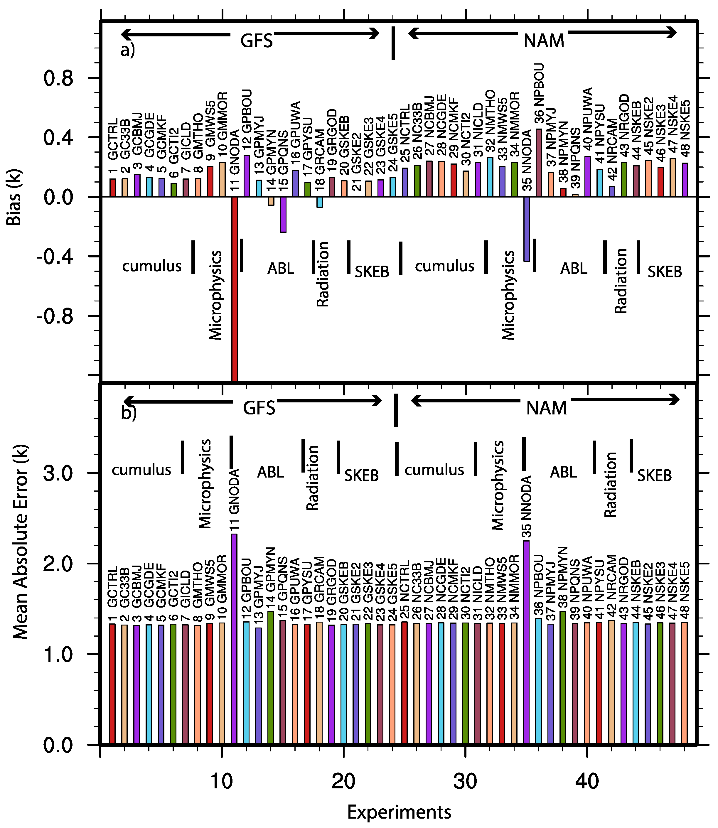
Bias, MAE and RMSE of T2 (Figure 6 and Figure 7) and bias and MAE of Q2 (Figure 8 and Figure 9), WS10 (Figure 10 and Figure 11) and wind direction (WD10) at 10 m (Figure 12 and Figure 13) for the January period are shown in the figures. The experiments without data assimilation stand out in all plots (not shown).
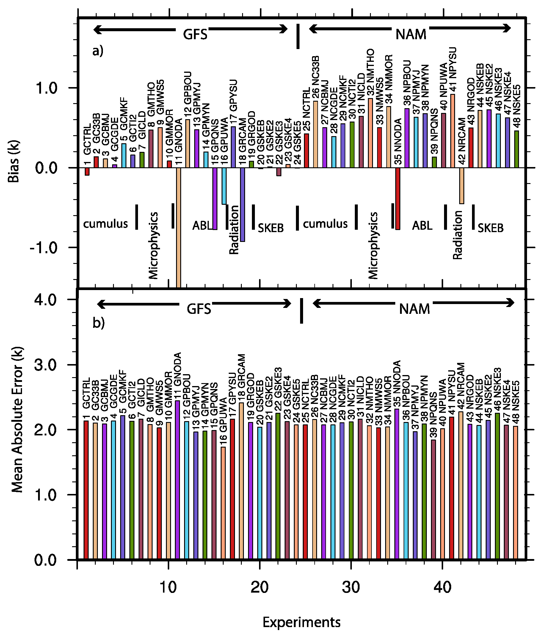
T2 is sensitive to microphysics and ABL schemes (Figure 6 and Figure 7). For the experiments with NAM as boundary and initial conditions, the difference in T2 bias is around 0.5 K among different ABL schemes. The YSU ABL scheme (control one) and MYN ABL scheme produce a smaller bias, while the BOU ABL scheme has larger bias at around 0.2 K. With GFS as the boundary and initial conditions, the range of bias is from −1.5 K–0.2 K. Results from the YSU ABL scheme and MYN ABL scheme are similar. The bias of the QNS ABL scheme is slightly higher. Among the different ABL schemes, more members with the GFS boundary and initial conditions are negative biases compared to those with the NAM boundary and initial conditions, which tend to have positive biases. Different shortwave radiation scheme can cause bias differences of around 0.2 K. The impacts of different cumulus parameterizations to T2 bias are similar; bias is positive for NAM boundary conditions, and the bias is negative for the GFS boundary conditions. Different microphysics can produce big differences in T2 bias, which reflects the impact of cloud on the surface temperature. The bias of the stochastic kinetic-energy backscatter (SKEB) scheme with the NAM boundary and initial conditions is slightly larger than the results from GFS boundary and initial conditions. MAE and RMSE among the different experiments with data assimilation are not meaningfully different, and the two metrics convey similar information (Figure 6). MAEs are all around 1.2 K and RMSEs around 1.8 K.
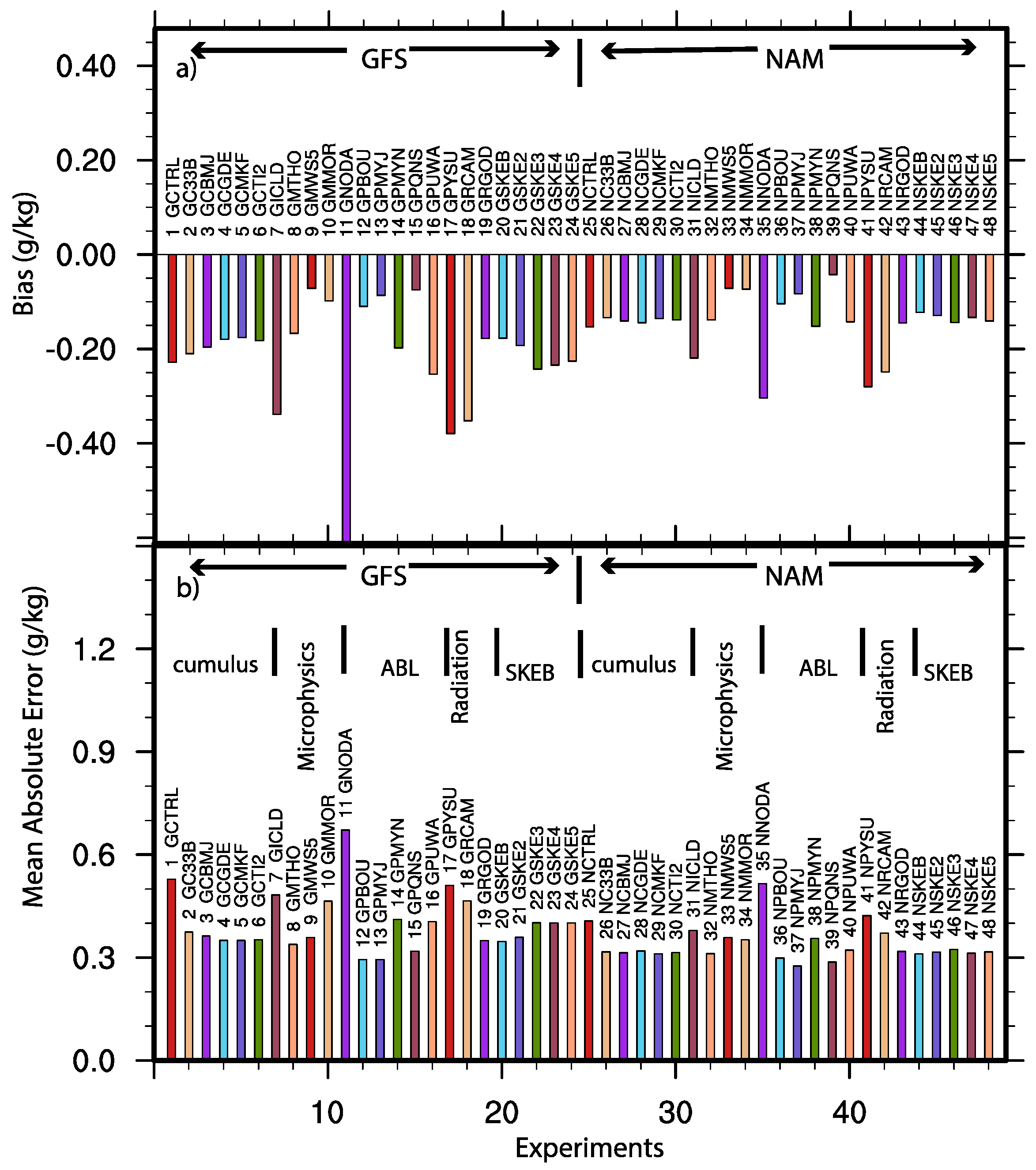
All members have a negative bias in Q2, and like the T2 bias, the Q2 bias is sensitive to different ABL schemes (Figure 8). With NAM as the boundary and initial conditions, Q2 bias ranges from −0.35 g/kg (11 NNODA) to −0.05 g/kg (39 NPQNS). With GFS as the boundary and initial conditions, Q2 bias ranges from −0.5 g/kg–−0.1 g/kg. Magnitudes of the negative biases are slightly higher from the GFS boundary and initial conditions than that from the NAM boundary and initial conditions. The spread of Q2 biases among different cumulus parameterizations and different microphysics is around 0.1 g/kg. The impacts of different SKEB schemes with different backscattered dissipation rates for potential temperature and stream function are similar. The differences in MAE are around 0.2 g/kg (Figure 7b). Values range from 0.4 g/kg–0.6 g/kg.
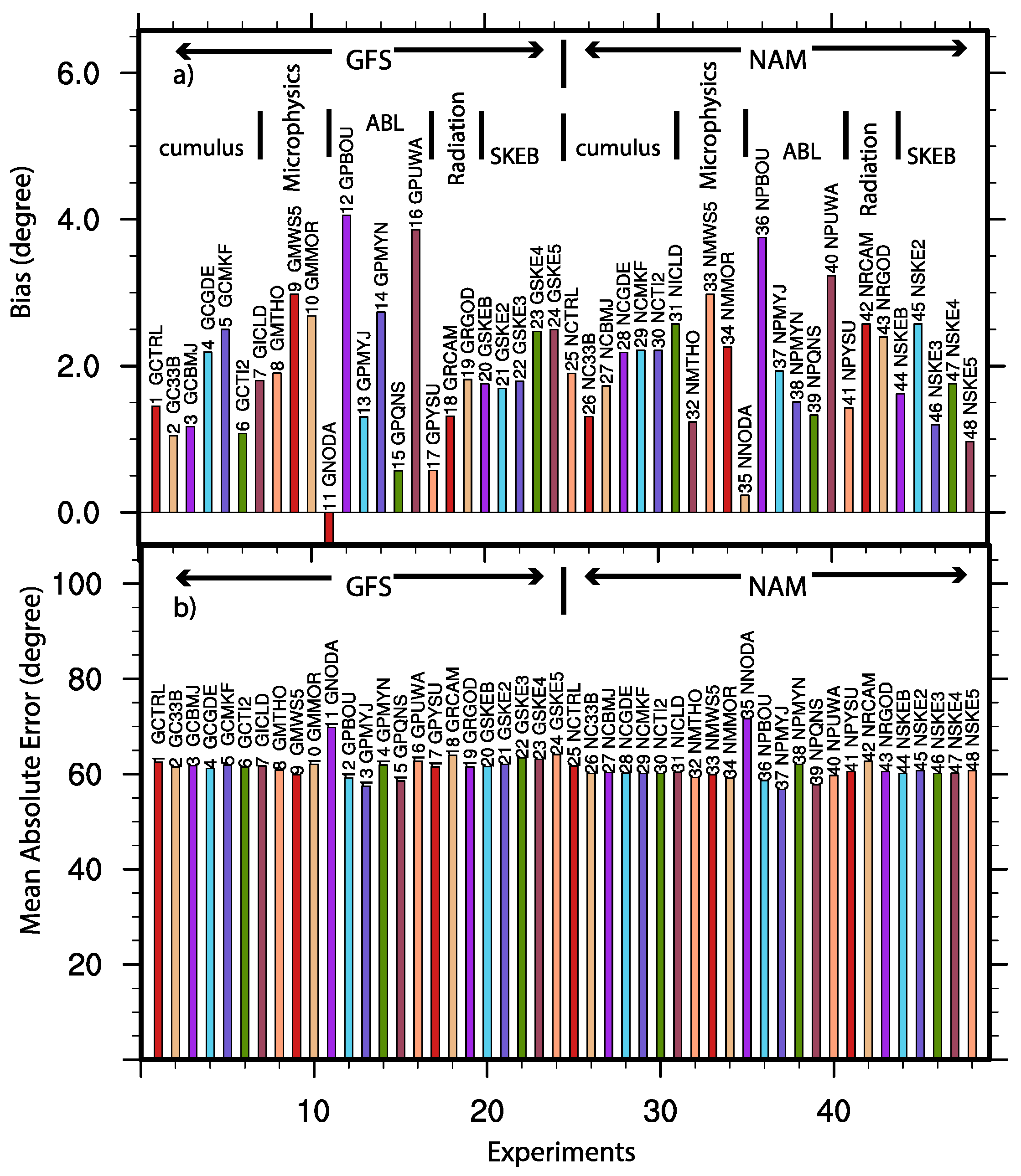
WS10 is most sensitive to the ABL scheme (Figure 9), more through bias than MAE, which does not vary much among experiments. The impacts of different microphysics and cumulus schemes on WS10 are comparatively small. All WS10 biases in the experiments are positive (Figure 9), ranging from 0.2 m s−1 (32 NMTHO) to 1.18 m s−1 (12 GPBOU). Performances with GFS and NAM boundary and initial conditions are similar. Both ABL schemes and microphysics have impacts on the WD10 bias (Figure 10). Biases range from −0.5°–4.0°. Experiments without data assimilation have the smallest biases. Differences between experiments with GFS and NAM as the boundary and initial conditions are very small. Differences in MAE among all experiments are minor; they are all around 65 degrees (Figure 10b).
Many of the sensitivities in July are similar to those in January (Figure 11 and Figure 12). Biases in forecasts of T2 vary from −1.25 K–0.2 K, and MAEs range from 1.4 K–2.5 K if including the experiments without data assimilation. The results for Q2, WS10 and WD10 are also similar (not shown).
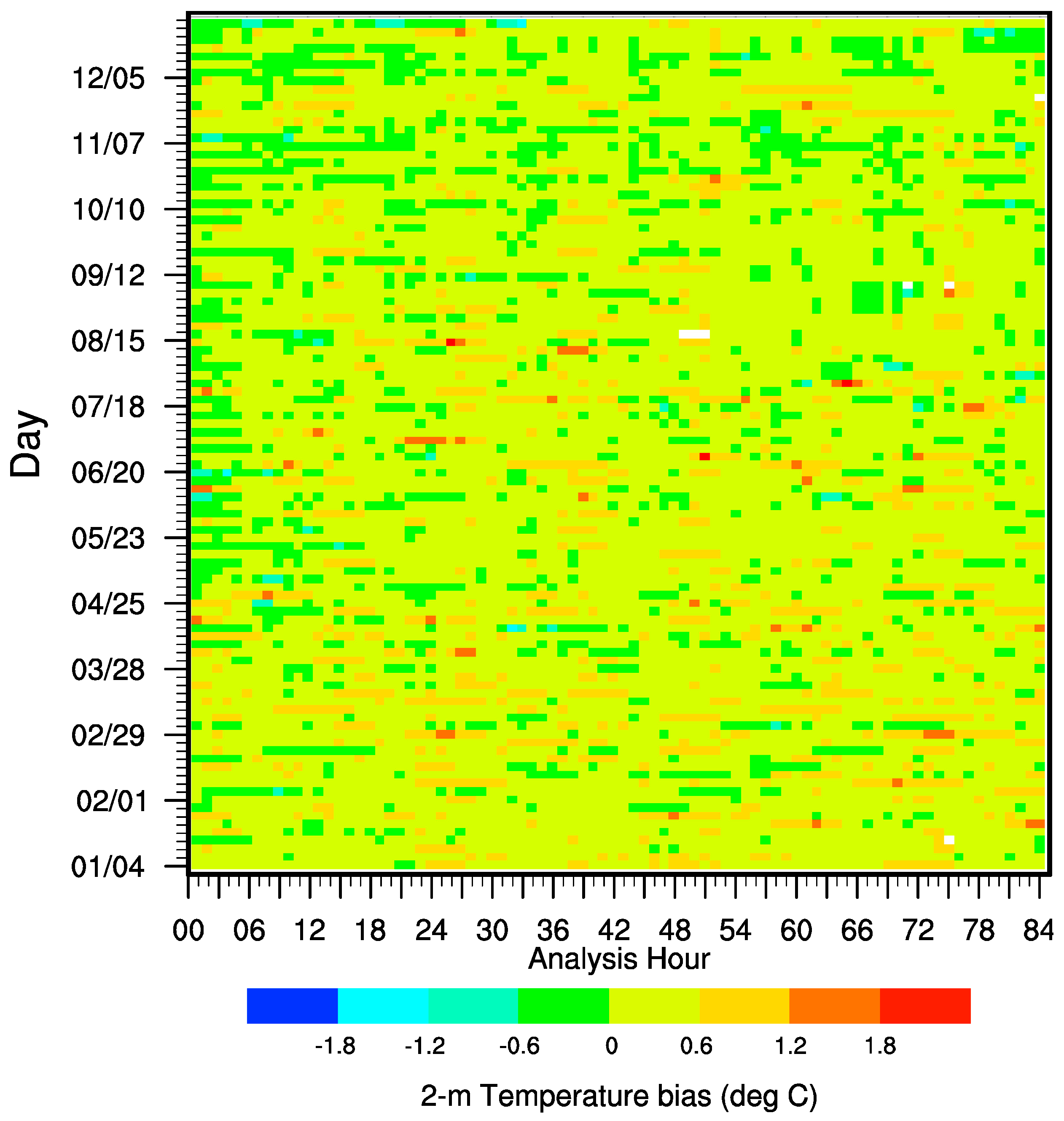
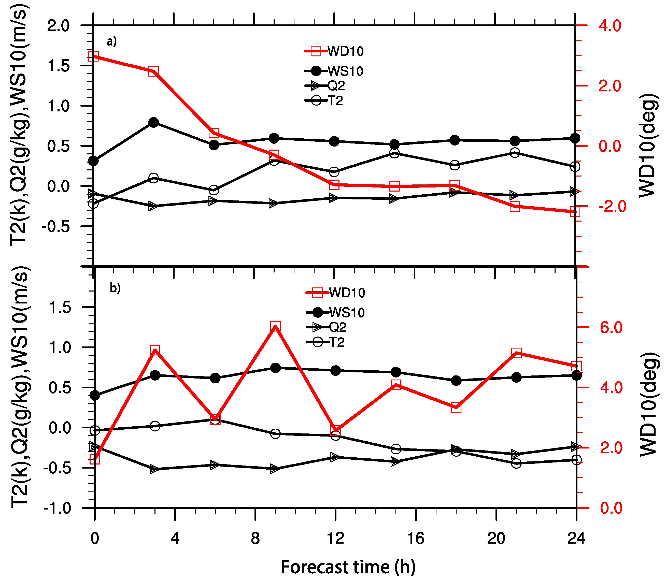
The sensitivity properties have similar results in winter and summer; however, the bias and MAE are bigger in summer than in winter (Figure 13). Both T2 and Q2 bias increase with time for the short-term forecast in summer. However, only Q2 bias increases with time for the short-term forecast in winter. T2 bias does not have a clear tendency in winter and ranges from 0.1 K–0.3 K, which is smaller than the values (0.2 K–0.5 K) in summer. Neither WS10 nor WD10 have a clear tendency during both winter and summer. The domain average bias in WS10 is around 0.5 m s−1 in both winter and summer. We also did a one-year run for the GFS control member, and basically, the results are similar. Figure 14 gives the variation of surface 2-m temperature bias in 2016. It tends to have a bias from −0.6 K–+0.6 K at most of the time. Data assimilation can also influence the sensitivity of different configurations since the data assimilation will force the model close to the observations, so the sensitivity will be reduced. Furthermore, sensitivities may depend on underlying surface properties, including topography, land use and soil types.
4. Conclusions
A mesoscale ensemble prediction system is used in this sensitivity study. The advantage of using an ensemble system to do the experiments is that they can be run in parallel. It is demonstrated that analyses and forecasts of T2, Q2, WS10 and WD10 can be sensitive to the ABL scheme. Q2 bias is consistently negative, and WS10 bias is consistently positive. T2 bias differs among the experiments by as much as 2.0 K. Q2 bias ranges from −0.5 g/kg–−0.05 g/kg, and WS10 bias ranges from 0.2 m s−1 (YSU ABL scheme with NAM boundary conditions) to 1.2 m s−1 (BOU ABL scheme with GFS boundary conditions). Different microphysics schemes produce big differences in T2 bias during the 1–24-h forecast period, which presumably reflects the impact of cloud on surface conditions. Microphysics can also influence WS10, but has relatively smaller impact on Q2. The choice of cumulus parameterization does not produce a clear signal in T2, Q2, WS10 and WD10. In some cases, the choice of boundary and initial conditions from GFS vs. NAM does have a noticeable impact on T2, Q2, WS10 and WD10. Through this sensitivity study, we have better knowledge of the sensitivities of different options of the model setting over the mountain areas in the western United States and get optimal settings for the real-time system based on the performances of different parameters. These optimal settings can also be used in an area similar to the Western United States. This study also provides useful information for ensemble member selections for the physical perturbations.
Acknowledgments
This work was funded by the U.S. Army Test and Evaluation Command through an Interagency Agreement with the National Science Foundation, which sponsors the National Center for Atmospheric Research.
Author Contributions
Y.L. and L.P. conceived of and designed the experiments. L.P. performed the experiments. L.P. and Y.L. analyzed the data. J.K. edited the manuscript. L.D.M. provided valuable comments and suggestions. G.R. contributed analysis tools.
Conflicts of Interest
The authors declare no conflict of interest.
References
- Shamarock, W.C.; Klemp, J.B.; Dudhia, J.; Gill, D.O.; Barker, D.M.; Wang, W.; Powers, J.G. A description of the Advanced Research WRF Version 2. NCAR Tech. Notes 2005. NCAR/TN-468+STR. [Google Scholar] [CrossRef]
- Carvalho, D.; Rocha, A.; Gomez-Gesteira, M.; Santos, C. A sensitivity study of the WRF model in wind simulation for an area of high wind energy. Environ. Model. Softw. 2012, 33, 23–34. [Google Scholar] [CrossRef]
- Banks, R.F.; Tiana-Alsina, J.; MaríaBaldasano, J.; Rocadenbosch, F.; Papayannis, A.; Solomos, S.; Tzanis, C.G. Sensitivity of boundary-layer variables to PBL schemes in the WRF model based on surface meteorological observations, lidar, and radiosondes during the HygrA-CD campaign. Atmos. Res. 2016, 176, 185–201. [Google Scholar] [CrossRef]
- Hu, X.M.; Nielsen-Gammon, J.M.; Zhang, F. Evaluation of three planetary boundary layer schemes in the WRF model. J. Appl. Meteorol. Climatol. 2010, 49, 1831–1844. [Google Scholar] [CrossRef]
- Kleczek, M.A.; Steeneveld, G.J.; Holtslag, A.A.M. Evaluation of the Weather Research and Forecasting mesoscale model for GABLS3: Impact of boundary-layer schemes, Boundary Conditions and Spin-Up. Bound.-Layer Meteorol. 2014, 152, 213–243. [Google Scholar] [CrossRef]
- Gómez-Navarro, J.J.; Raible, C.C.; Die, S. Sensitivity of the WRF model to PBL parameterizations and nesting techniques: Evaluation of wind storms over complex terrain. Geosci. Model Dev. 2014, 8, 3349–3363. [Google Scholar] [CrossRef] [Green Version]
- Hariprasad, K.B.R.R.; Srinivas, C.V.; Bagavath Singh, A.; Vijaya Bhaskara Rao, S.; Baskaran, R.; Venkatraman, B. Numerical simulation and intercomparison of boundary layer structure with different PBL schemes in WRF using experimental observations at a tropical site. Atmos. Res. 2014, 145, 27–44. [Google Scholar] [CrossRef]
- Frediani, M.E.B.; Hacker, J.P.; Anagnostou, E.N.; Hopson, T. Evaluation of PBL Parameterizations for Modeling Surface Wind Speed during Storms in the Northeast United States. Weather Forecast. 2016, 31, 1511–1528. [Google Scholar] [CrossRef]
- Tymvios, F.; Charalambous, D.; Michaelides, S.; Lelieveld, J. Intercomparison of boundary layer parameterizations for summer conditions in the eastern Mediterranean island of Cyprus using the WRF—ARW model. Atmos. Res. 2017. [Google Scholar] [CrossRef]
- Hahmann, A.N.; Vincent, C.L.; Peña, A.; Lange, J.; Hasager, C.B. Wind climate estimation using WRF model output: Method and model sensitivities over the sea. Int. J. Climatol. 2015, 35, 3422–3439. [Google Scholar] [CrossRef]
- Ruiz, J.J.; Saulo, C. WRF Model Sensitivity to Choice of Parameterization over South America: Validation against Surface Variables. Mon. Weather Rev. 2010, 138, 3342–3355. [Google Scholar] [CrossRef]
- Chadee, X.; Seegobin, N.; Clarke, R. Optimizing the Weather Research and Forecasting (WRF) Model for Mapping the Near-Surface Wind Resources over the Southernmost Caribbean Islands of Trinidad and Tobago. Energies 2017, 10, 931. [Google Scholar] [CrossRef]
- Santos-Alamillos, F.J.; Pozo-Vázquez, D.; Ruiz-Arias, J.A.; Lara-Fanego, V.; Tovar-Pescador, J. Analysis of WRF Model Wind Estimate Sensitivity to Physics Parameterization Choice and Terrain Representation in Andalusia (Southern Spain). J. Appl. Meteorol. Climatol. 2013, 52, 1592–1609. [Google Scholar] [CrossRef]
- Di, Z.; Duan, Q.; Gong, W.; Wang, C.; Gan, Y.; Quan, J.; Li, J.; Miao, C.; Ye, A.; Tong, C. Assessing WRF model parameter sensitivity: A case study with 5 day summer precipitation forecasting in the Greater Beijing Area. Geophys. Res. Lett. 2015, 42, 579–587. [Google Scholar] [CrossRef]
- Pei, L.; Moore, N.; Zhong, S.; Luo, L.; Hyndman, D.W.; Heilman, W.E.; Gao, Z. WRF model sensitivity to land surface model and cumulus parameterization under short-term climate extremes over the southern Great Plains of the United States. J. Clim. 2014, 27, 7703–7724. [Google Scholar] [CrossRef]
- Rajeevan, M.; Kesarkar, A.; Thampi, S.B.; Rao, T.N.; Radhakrishna, B.; Rajasekhar, M. Sensitivity of WRF cloud microphysics to simulations of a severe thunderstorm event over Southeast India. Ann. Geophys. 2010, 28, 603–619. [Google Scholar] [CrossRef]
- Hong, S.-Y.; Lim, K.-S.S.; Kim, J.-H.; Lim, J.-O.J.; Dudhia, J. Sensitivity Study of Cloud-Resolving Convective Simulations with WRF Using Two Bulk Microphysical Parameterizations: Ice-Phase Microphysics versus Sedimentation Effects. J. Appl. Meteorol. Clim. 2009, 48, 61–76. [Google Scholar] [CrossRef]
- Patil, R.; Kumar, P.P. WRF model sensitivity for simulating intense western disturbances over North West India, Model. Earth Syst. Environ. 2016, 2, 1–15. [Google Scholar] [CrossRef]
- Orr, A.; Listowski, C.; Couttet, M.; Collier, E.; Immerzeel, W.; Deb, P.; Bannister, D. Sensitivity of simulated summer monsoonal precipitation in Langtang Valley, Himalaya, to cloud microphysics schemes in WRF. J. Geophy. Res. Atmos. 2017, 122, 6298–6318. [Google Scholar] [CrossRef]
- García-Díez, M.; Fernández, J.; Vautard, R. An RCM multi-physics ensemble over Europe: Multi-variable evaluation to avoid error compensation. Clim. Dyn. 2015, 45, 3141–3156. [Google Scholar] [CrossRef]
- Jerez, S.; Montavez, J.P.; Jimenez-Guerrero, P.; Gomez-Navarro, J.J.; Lorente-Plazas, R.; Zorita, E. A multi-physics ensemble of present-day climate regional simulations over the Iberian Peninsula. Clim. Dyn. 2013, 40, 3023–4306. [Google Scholar] [CrossRef]
- Di Luca, A.; Flaounas, E.; Drobinski, P.; Brossier, C.L. The atmospheric component of the Mediterranean Sea water budget in a WRF multi-physics ensemble and observations. Clim. Dyn. 2014, 43, 2349–2375. [Google Scholar] [CrossRef]
- Zeng, X.-M.; Wang, N.; Wang, Y.; Zheng, Y.; Zhou, Z.; Wang, G.; Chen, C.; Liu, H. WRF-simulated sensitivity to land surface schemes in short and medium ranges for a high-temperature event in East China: A comparative study. J. Adv. Model. Earth Syst. 2015, 7, 1305–1325. [Google Scholar] [CrossRef]
- Nemunaitis-Berry, K.L.; Klein, P.M.; Basara, J.B.; Fedorovich, E. Sensitivity of Predictions of the Urban Surface Energy Balance and Heat Island to Variations of Urban Canopy Parameters in Simulations with the WRF Model. J. Appl. Meteorol. Clim. 2017, 56, 573–595. [Google Scholar] [CrossRef]
- Zeng, X.-M.; Wang, M.; Wang, N.; Yi, X.; Chen, C.; Zhou, Z.; Wang, G.; Zheng, Y. Assessing simulated summer 10-m wind speed over China: influencing processes and sensitivities to land surface schemes. Clim. Dyn. 2017. [Google Scholar] [CrossRef]
- Lorente-Plazas, R.; Jiménez, P.A.; Dudhia, J.; Montávez, J.P. Evaluating and Improving the Impact of the Atmospheric Stability and Orography on Surface Winds in the WRF Model. Mon. Weather Rev. 2016, 144, 2685–2693. [Google Scholar] [CrossRef]
- Jee, J.-B.; Kim, S. Sensitivity Study on High-Resolution Numerical Modeling of Static Topographic Data. Atmosphere 2016, 7, 86. [Google Scholar] [CrossRef]
- Santos-Alamillos, F.J.; Pozo-Vázquez, D.; Ruiz-Arias, J.A.; Tovar-Pescador, J. Influence of land-use misrepresentation on the accuracy of WRF wind estimates: Evaluation of GLCC and CORINE land-use maps in southern Spain. Atmos. Res. 2015, 157, 17–28. [Google Scholar] [CrossRef]
- Pan, L.; Liu, Y.; Li, L.; Jiang, J.; Cheng, W.; Roux, G. Impact of four-dimensional data assimilation (FDDA) on urban climate analysis. J. Adv. Model. Earth Syst. 2015, 7, 1997–2011. [Google Scholar] [CrossRef]
- Knievel, J.; Liu, Y.; Hopson, T.; Shaw, J.; Halvorson, S.; Fisher, H.; Roux, G.; Sheu, R.; Pan, L.; Wu, W.; et al. Mesoscale ensemble weather prediction at U. S. Army Dugway Proving Ground, Utah. Weather Forecast. 2017, 32, 2195–2216. [Google Scholar] [CrossRef]
- Wicker, L.J.; Skamarock, W.C. Time splitting methods for elastic models using forward time schemes. Mon. Weather Rev. 2002, 130, 729–747. [Google Scholar] [CrossRef]
- Klemp, J.B.; Skamarock, W.C.; Dudhia, J. Conservative split-explicit time integration methods for the compressible nonhydrostatic equations. Mon. Weather Rev. 2007, 135, 2897–2913. [Google Scholar] [CrossRef]
- Knievel, J.C.; Bryan, G.H.; Hacker, J.P. Explicit numerical diffusion in the WRF Model. Mon. Weather Rev. 2007, 135, 3808–3824. [Google Scholar] [CrossRef]
- Kain, J.S.; Fritsch, J.M. A one-dimensional entraining detraining plume model and its application in convective parameterization. J. Atmos. Sci. 1990, 47, 2784–2802. [Google Scholar] [CrossRef]
- Lin, Y.-L.; Farley, R.D.; Orville, H.D. Bulk parameterization of the snow field in a cloud model. J. Clim. Appl. Meteorol. 1983, 22, 1065–1092. [Google Scholar] [CrossRef]
- Mlawer, E.J.; Taubman, S.J.; Brown, P.D.; Iacono, M.J.; Clough, S.A. Radiative transfer for inhomogeneous atmospheres: RRTM, a validated correlated-k model for the longwave. J. Geophys. Res. 1997, 102, 16663–16682. [Google Scholar] [CrossRef]
- Dudhia, J. Numerical study of convection observed during the Winter Monsoon Experiment using a mesoscale two-dimensional model. J. Atmos. Sci. 1989, 46, 3077–3107. [Google Scholar] [CrossRef]
- Hong, S.-Y.; Noh, Y.; Dudhia, J. A new vertical diffusion package with an explicit treatment of entrainment processes. Mon. Weather Rev. 2006, 134, 2318–2341. [Google Scholar] [CrossRef]
- Niu, G.-Y.; Yang, Z.-L.; Mitchell, K.E.; Chen, F.; Ek, M.B.; Barlage, M.; Kumar, A.; Manning, K.; Niyogi, D.; Rosero, E.; et al. The community Noah land surface model with multiparameterization options (Noah-MP): 1. Model description and evaluation with local-scale measurements. J. Geophys. Res. 2011, 116, D12109. [Google Scholar] [CrossRef]
- Skamarock, W.C.; Klemp, J.B.; Dudhia, J.; Gill, D.O.; Barker, D.M.; Duda, M.G.; Wang, W.; Powers, J.G. A description of the Advanced Research WRF Version 3. NCAR Tech. Notes 2008. NCAR/TN-475+STR. [Google Scholar] [CrossRef]
Figure 1.
Model topography of (a) Domain 1, (b) Domain 2 and (c) Domain 3 and surface stations (white dots) in Domain 3 (c). The area within the green rectangle in (a) is Domain 2 (D2), and the area within the white rectangle is Domain 3 (D3). Topography (m above mean sea level) is shaded.
Figure 1.
Model topography of (a) Domain 1, (b) Domain 2 and (c) Domain 3 and surface stations (white dots) in Domain 3 (c). The area within the green rectangle in (a) is Domain 2 (D2), and the area within the white rectangle is Domain 3 (D3). Topography (m above mean sea level) is shaded.

Figure 2.
Boxplot of the averages on Domain 3 of (a) correlation and (b) normalized standard deviation of air temperature at 2 m above ground level (T2) (red), Q2 (blue), and wind speed (WS) (green); and (c) Taylor diagram of the analysis during the one-week study period in January 2016. Numbers refer to experiments.

Figure 3.
Same as Figure 2, but for 1–24-h forecasts.
Figure 3.
Same as Figure 2, but for 1–24-h forecasts.

Figure 4.
Same as Figure 2, but for the one-week study period in July.
Figure 4.
Same as Figure 2, but for the one-week study period in July.

Figure 5.
Same as Figure 3, but for the one-week study period in July.
Figure 5.
Same as Figure 3, but for the one-week study period in July.
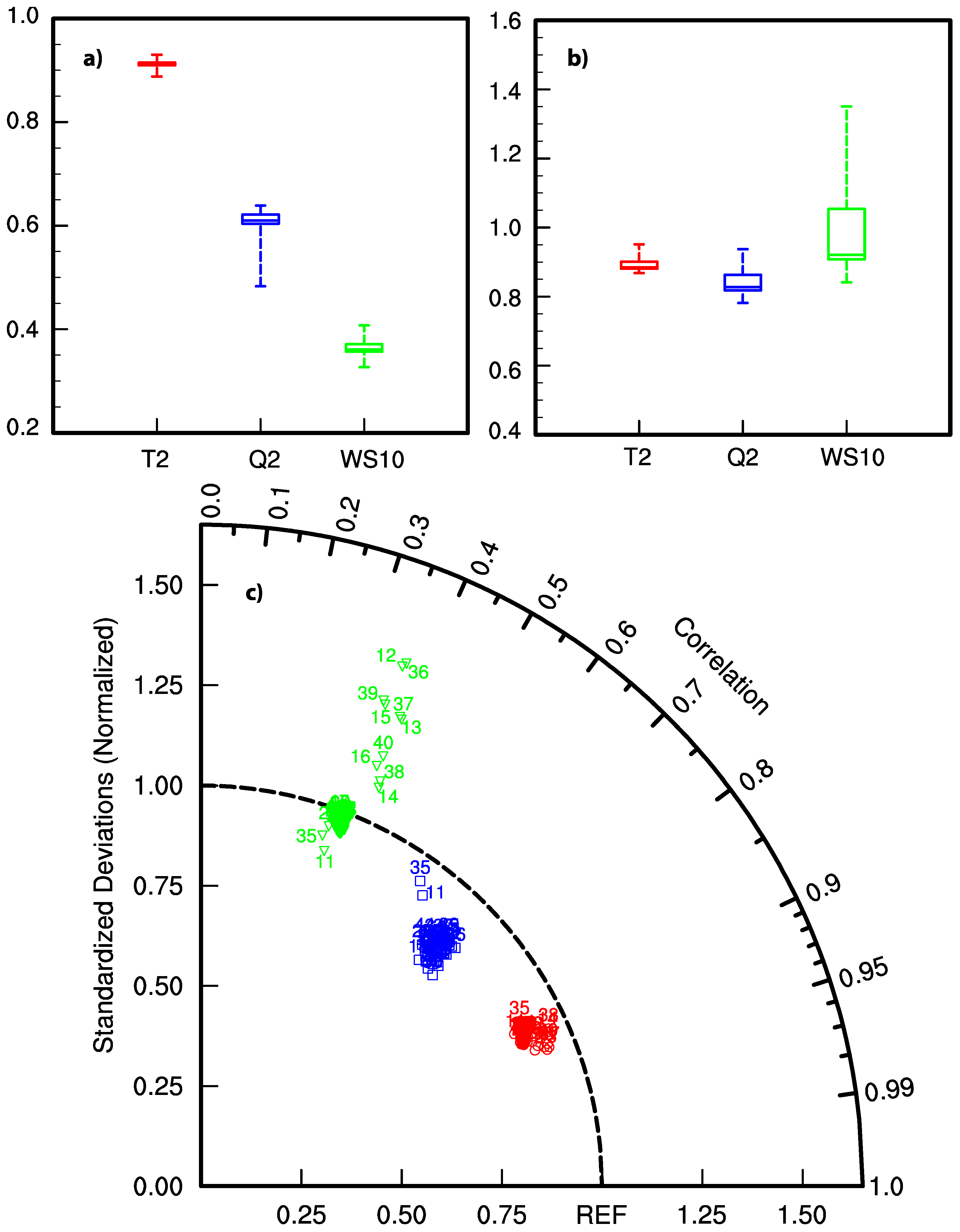
Figure 6.
Averages on Domain 3 of (a) bias, (b) MAE and (c) RMSE in T2 from analyses during the one-week study period in January. The unit is K.
Figure 6.
Averages on Domain 3 of (a) bias, (b) MAE and (c) RMSE in T2 from analyses during the one-week study period in January. The unit is K.
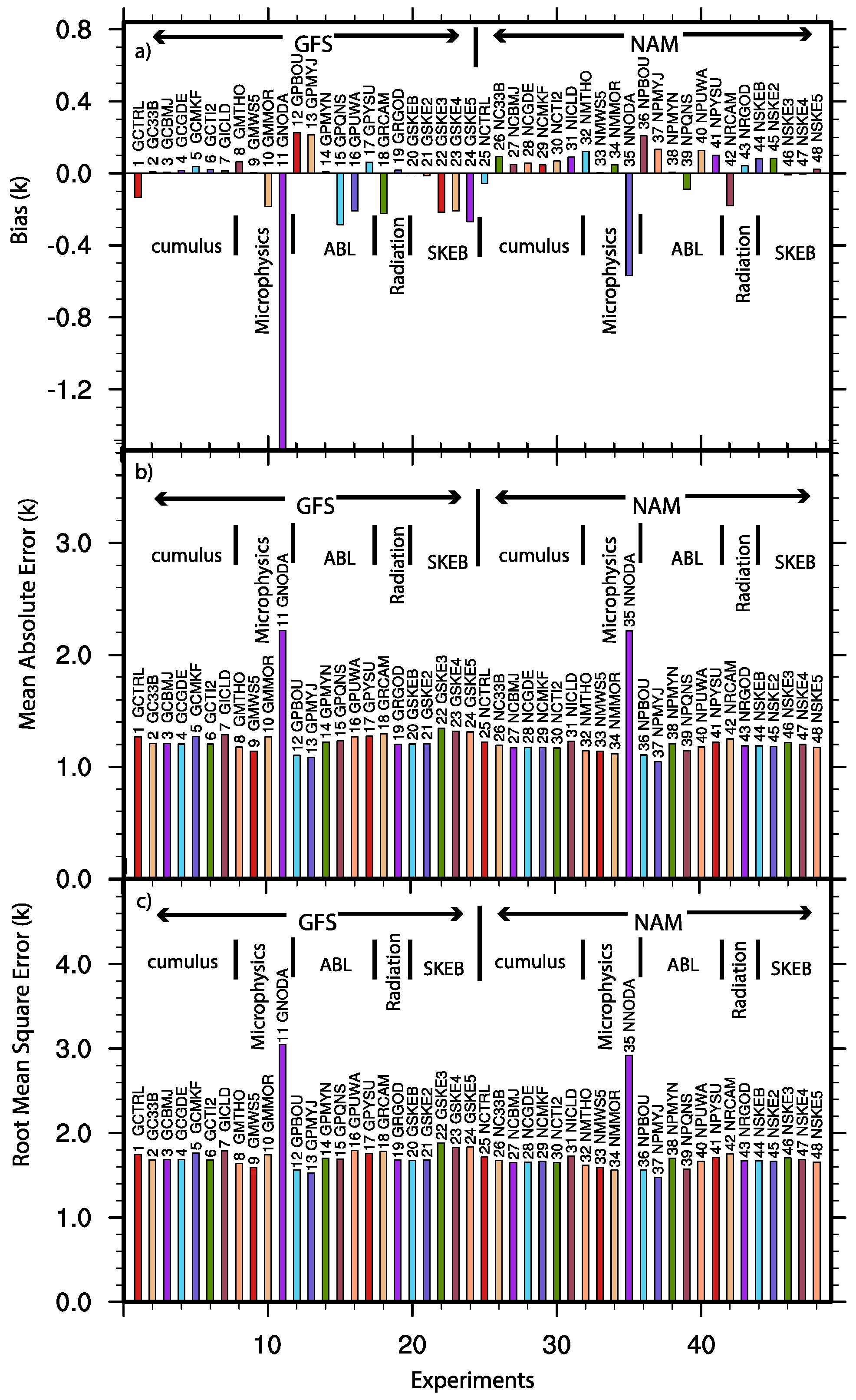
Figure 7.
Averages on Domain 3 of (a) bias and (b) MAE in T2 from 1–24-h forecasts during the one-week study period in January. The unit is K.
Figure 7.
Averages on Domain 3 of (a) bias and (b) MAE in T2 from 1–24-h forecasts during the one-week study period in January. The unit is K.

Figure 8.
Averages on Domain 3 of (a) bias and (b) MAE in Q2 from analyses during the one-week study period in January. The unit is g/kg.
Figure 8.
Averages on Domain 3 of (a) bias and (b) MAE in Q2 from analyses during the one-week study period in January. The unit is g/kg.

Figure 9.
Averages on Domain 3 of (a) bias and (b) MAE in WS10 from analyses during the one-week study period in January. The unit is m s−1.
Figure 9.
Averages on Domain 3 of (a) bias and (b) MAE in WS10 from analyses during the one-week study period in January. The unit is m s−1.
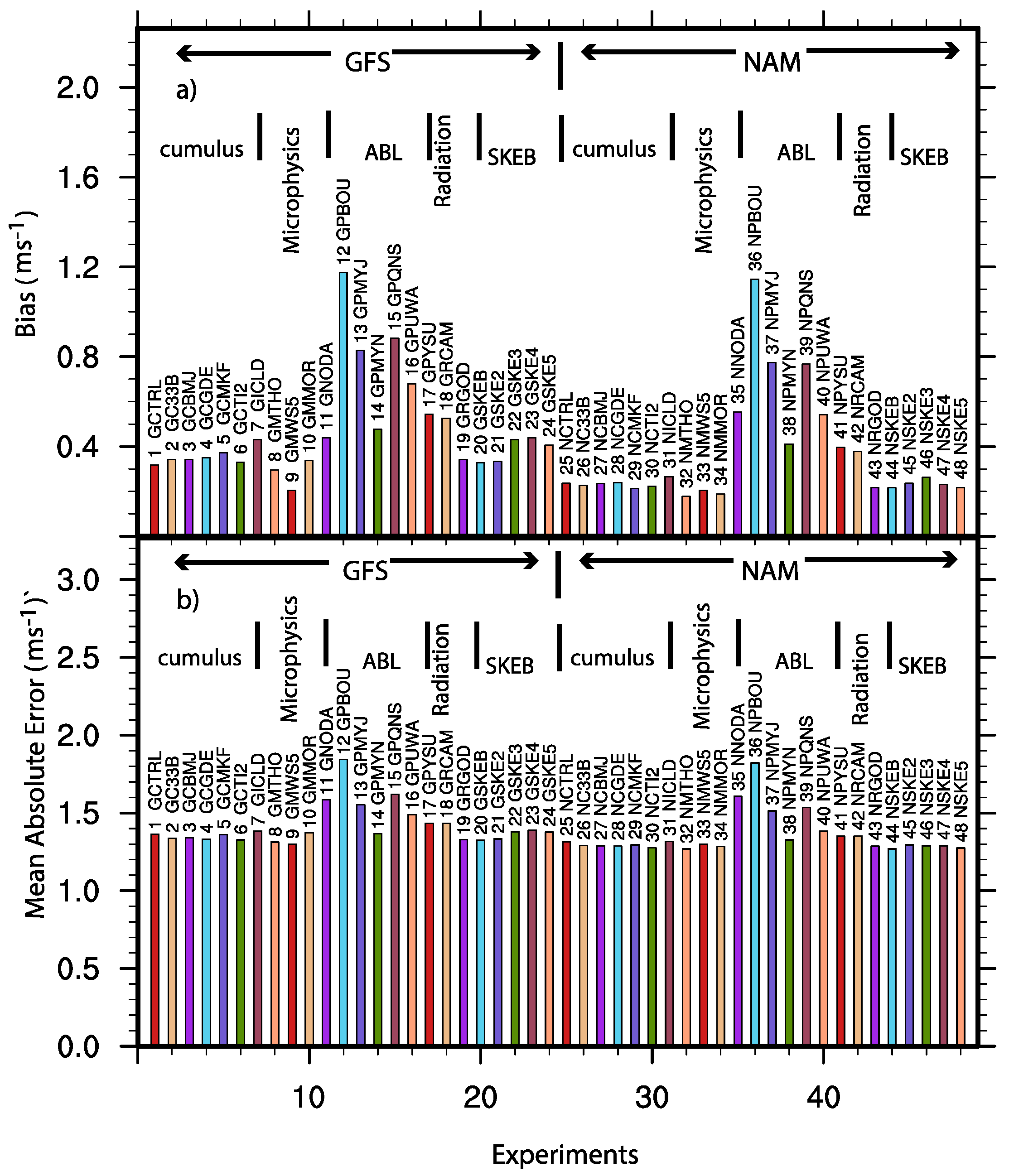
Figure 10.
Averages on Domain 3 of (a) bias and (b) MAE in wind direction at 10 m (WD10) from analyses during the one-week study period in January. The unit is degrees.
Figure 10.
Averages on Domain 3 of (a) bias and (b) MAE in wind direction at 10 m (WD10) from analyses during the one-week study period in January. The unit is degrees.

Figure 11.
Averages on Domain 3 of (a) bias and (b) MAE in T2 from analyses during the one-week study period in July.
Figure 11.
Averages on Domain 3 of (a) bias and (b) MAE in T2 from analyses during the one-week study period in July.

Figure 12.
Averages on Domain 3 of (a) bias and (b) MAE in T2 from forecasts during the one-week study period in July.
Figure 12.
Averages on Domain 3 of (a) bias and (b) MAE in T2 from forecasts during the one-week study period in July.
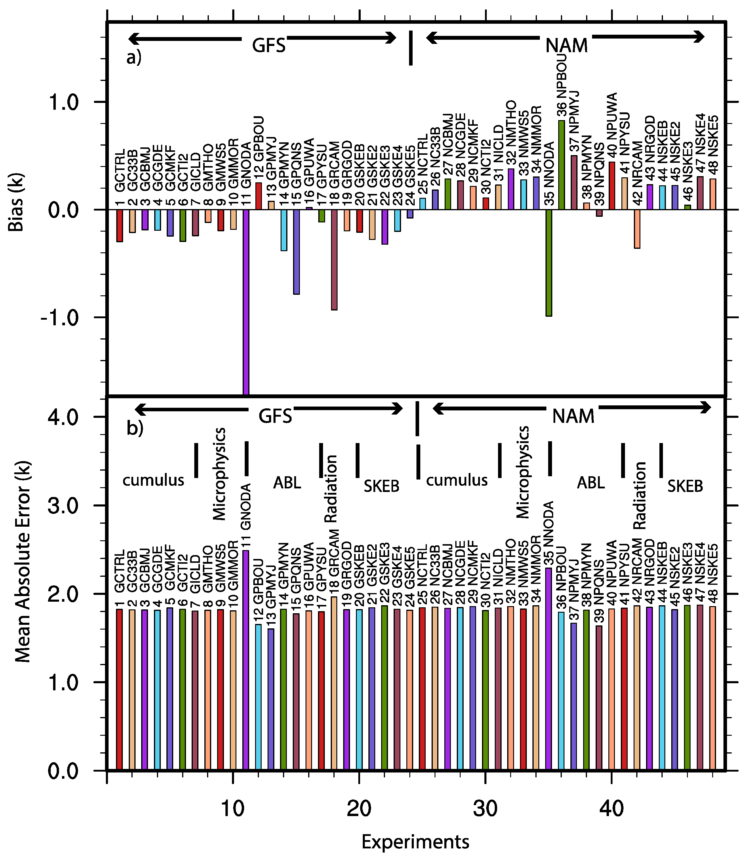
Figure 13.
Bias in T2 (black circles), Q2 (black triangle), WS10 (black dot) and WD10 (red square) as a function of forecast lead time (h) from control forecasts in (a) January and (b) July.
Figure 13.
Bias in T2 (black circles), Q2 (black triangle), WS10 (black dot) and WD10 (red square) as a function of forecast lead time (h) from control forecasts in (a) January and (b) July.

Figure 14.
Domain averaged 2-m temperature bias in 2016 for the GFS control member. The empty part (white) corresponds to the missing value.
Figure 14.
Domain averaged 2-m temperature bias in 2016 for the GFS control member. The empty part (white) corresponds to the missing value.

Table 1.
List of experiments. YSU: Yonsei University; GFS: Global Forecast System; NAM: North American Mesoscale Forecast System.
Table 1.
List of experiments. YSU: Yonsei University; GFS: Global Forecast System; NAM: North American Mesoscale Forecast System.
| Experiment | Descriptions of the Experiment Setting | Abbreviation | |
|---|---|---|---|
| Descriptions | Boundary Conditions | ||
| 1 | Control run with YSU ABL scheme, Kain–Fritsch cumulus scheme, single momentum 6-class microphysics, Dudhia Shortwave | GFS | GCTRL |
| 2 | Betts–Miller–Janjic cumulus scheme including D3 | GFS | GC33B |
| 3 | Betts–Miller–Janjic cumulus scheme | GFS | GCBMJ |
| 4 | Grell–Devenyi ensemble cumulus scheme | GFS | GCGDE |
| 5 | Multi-scale Kain–Fritsch cumulus scheme | GFS | GCMKF |
| 6 | New Tiedtke cumulus scheme | GFS | GCTI2 |
| 7 | Relative Humidity (RH)-based method for cloud fraction | GFS | GICLD |
| 8 | Thompson microphysics | GFS | GMTHO |
| 9 | WRF Double Momentum (WDM) 5-class scheme | GFS | GMWS5 |
| 10 | Morrison microphysics scheme | GFS | GMMOR |
| 11 | Similar to experiment 1 (GCTRL) except without data assimilation | GFS | GNODA |
| 12 | Bougeault and Lacarrere (BOU) ABL scheme | GFS | GPBOU |
| 13 | Mellor–Yamada–Janjic (Eta) Turbulent Kinetic Energy (TKE) ABL scheme | GFS | GPMYJ |
| 14 | Mellor-Yamada-Nakanishi-Niino (MYN) 2.5 level TKE ABL scheme | GFS | GPMYN |
| 15 | Quasi-Normal Scale Elimination (QNS) ABL scheme | GFS | GPQNS |
| 16 | University of Washington (UW) (Bretherton and Park) ABL scheme | GFS | GPUWA |
| 17 | YSU ABL scheme with modified mixing | GFS | GPYSU |
| 18 | Community Atmospheric Model (CAM) short wave radiation | GFS | GRCAM |
| 19 | Goddard shortwave scheme | GFS | GRGOD |
| 20 | Stochastic kinetic-energy backscatter Scheme (SKEBS) 1 | GFS | GSKEB |
| 21 | Stochastic kinetic-energy backscatter Scheme (SKEBS) 2 | GFS | GSKE2 |
| 22 | Stochastic kinetic-energy backscatter Scheme (SKEBS) 3 | GFS | GSKE3 |
| 23 | Stochastic kinetic-energy backscatter Scheme (SKEBS) 4 | GFS | GSKE4 |
| 24 | Stochastic kinetic-energy backscatter Scheme (SKEBS) 5 | GFS | GSKE5 |
| 25 | Control run with YSU ABL scheme, Kain–Fritsch cumulus scheme, single momentum 6-class microphysics scheme | NAM | NCTRL |
| 26 | Betts–Miller–Janjic cumulus scheme | NAM | NC33B |
| 27 | Betts–Miller–Janjic cumulus scheme | NAM | NCBMJ |
| 28 | Grell–Devenyi ensemble cumulus scheme | NAM | NCGDE |
| 29 | Multi-scale Kain–Fritsch cumulus scheme | NAM | NCMKF |
| 30 | New Tiedtke cumulus scheme | NAM | NCTI2 |
| 31 | RH-based method for cloud fraction | NAM | NICLD |
| 32 | Thompson microphysics | NAM | NMTHO |
| 33 | WDM 5-class scheme | NAM | NMWS5 |
| 34 | Morrison microphysics scheme | NAM | NMMOR |
| 35 | Similar to experiment 25 (NCTRL) except without data assimilation | NAM | NNODA |
| 36 | Bougeault and Lacarrere (BouLac) ABL scheme | NAM | NPBOU |
| 37 | Mellor–Yamada–Janjic (Eta) TKE ABL scheme | NAM | NPMYJ |
| 38 | MYNN 2.5 level TKE ABL scheme | NAM | NPMYN |
| 39 | Quasi-Normal Scale Elimination ABL scheme | NAM | NPQNS |
| 40 | UW (Bretherton and Park) ABL scheme | NAM | NPUWA |
| 41 | YSU ABL scheme with modified mixing | NAM | NPYSU |
| 42 | CAM short wave radiation | NAM | NRCAM |
| 43 | Goddard shortwave scheme | NAM | NRGOD |
| 44 | Stochastic kinetic-energy backscatter (SKEB) Scheme 1 | NAM | NSKEB |
| 45 | Stochastic kinetic-energy backscatter (SKEB) Scheme 2 | NAM | NSKE2 |
| 46 | Stochastic kinetic-energy backscatter (SKEB) Scheme 3 | NAM | NSKE3 |
| 47 | Stochastic kinetic-energy backscatter (SKEB) Scheme 4 | NAM | NSKE4 |
| 48 | Stochastic kinetic-energy backscatter Scheme (SKEBS) 5 | NAM | NSKE5 |
© 2018 by the authors. Licensee MDPI, Basel, Switzerland. This article is an open access article distributed under the terms and conditions of the Creative Commons Attribution (CC BY) license (http://creativecommons.org/licenses/by/4.0/).
Share and Cite
MDPI and ACS Style
Pan, L.; Liu, Y.; Knievel, J.C.; Delle Monache, L.; Roux, G. Evaluations of WRF Sensitivities in Surface Simulations with an Ensemble Prediction System. Atmosphere 2018, 9, 106. https://doi.org/10.3390/atmos9030106
AMA Style
Pan L, Liu Y, Knievel JC, Delle Monache L, Roux G. Evaluations of WRF Sensitivities in Surface Simulations with an Ensemble Prediction System. Atmosphere. 2018; 9(3):106. https://doi.org/10.3390/atmos9030106
Chicago/Turabian StylePan, Linlin, Yubao Liu, Jason C. Knievel, Luca Delle Monache, and Gregory Roux. 2018. "Evaluations of WRF Sensitivities in Surface Simulations with an Ensemble Prediction System" Atmosphere 9, no. 3: 106. https://doi.org/10.3390/atmos9030106
Note that from the first issue of 2016, this journal uses article numbers instead of page numbers. See further details here.