Article

Validation Study for an Atmospheric Dispersion Model, Using Effective Source Heights Determined from Wind Tunnel Experiments in Nuclear Safety Analysis

1
Nikkenn Sekkei Ltd., Tokyo 102-8117, Japan
2
Institute of Industrial Science, The University of Tokyo, Tokyo 153-8505, Japan
3
Faculty of Engineering & Physical Sciences, University of Surrey, Surrey GU2 7XH, UK
*
Author to whom correspondence should be addressed.
Atmosphere 2018, 9(3), 111; https://doi.org/10.3390/atmos9030111
Submission received: 14 February 2018 / Revised: 12 March 2018 / Accepted: 14 March 2018 / Published: 18 March 2018
(This article belongs to the Section Air Quality)

Abstract

:
For more than fifty years, atmospheric dispersion predictions based on the joint use of a Gaussian plume model and wind tunnel experiments have been applied in both Japan and the U.K. for the evaluation of public radiation exposure in nuclear safety analysis. The effective source height used in the Gaussian model is determined from ground-level concentration data obtained by a wind tunnel experiment using a scaled terrain and site model. In the present paper, the concentrations calculated by this method are compared with data observed over complex terrain in the field, under a number of meteorological conditions. Good agreement was confirmed in near-neutral and unstable stabilities. However, it was found to be necessary to reduce the effective source height by 50% in order to achieve a conservative estimation of the field observations in a stable atmosphere.

1. Introduction

Prior to the construction of a nuclear power station, electric power companies in Japan evaluate potential public radiation exposure by using a combined atmospheric dispersion model, based on a Gaussian plume model and wind tunnel experiments. For over fifty years, this approach to nuclear safety analysis has been followed, based on the nuclear regulatory rules [1]. Similar methods have been applied elsewhere, for example in the U.K. [2].
Because the basic Gaussian plume model assumes atmospheric dispersion over flat terrain, an effective source height (He’), which is different from the conventional effective stack height (He = stack height + plume rise), has been used in nuclear safety analysis in Japan and the U.K. to account for terrain and building effects. Concentration data obtained in wind tunnel experiments with a scaled terrain model provide one basis for determining He’ [3]. Other adjustments that are applied include the determination of the effects of plume rise on the effective plume height, either by applying semi-empirical rise formulae, or again, from wind tunnel simulations. However, here we concentrate on the terrain correction.
The validity of applying the combined Gaussian plume and wind tunnel modelling to dispersion over complex terrain has not been extensively tested by field dispersion experiments under general meteorological conditions (especially non-neutral atmospheric stabilities), because there are very few observed data on concentrations over complex terrain under non-neutral atmospheric conditions. To help remedy the situation, we compared predictions from the combined methods with observed data from field dispersion tests around Mt. Tsukuba, near Tokyo, Japan [4]. This allowed us to evaluate the validity of the method for regulatory use under a range of meteorological conditions: neutral, stable, and unstable.

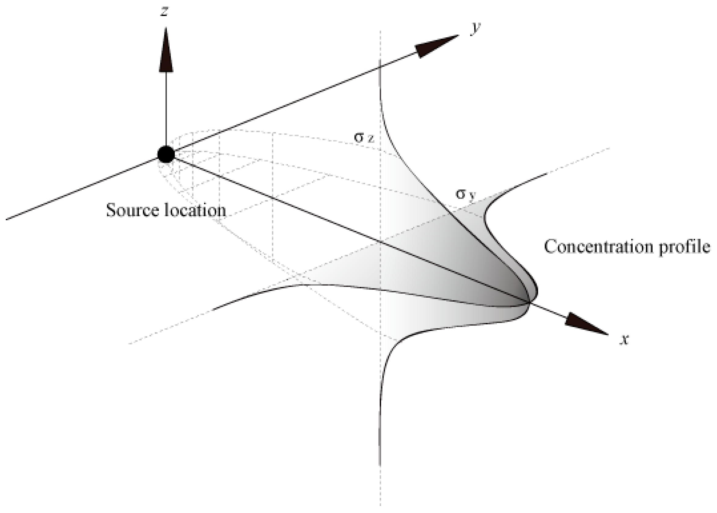
2. The Effective Source Height Gaussian Plume Model

2.1. Japanese Experience

The Gaussian plume model can be derived from the fundamental equation of gas dispersion, under the assumption of a steady emission into uniform air flow and turbulence over flat terrain, giving:
C = Q 2 π   U σ y σ z exp { y 2 2 σ y 2 } [ exp { ( He + z ) 2 2 σ z 2 } + exp { ( He z ) 2 2 σ z 2 } ]
where C is the pollutant concentration, Q the emission rate, U the mean wind velocity, σ y the lateral plume spread, σ z the vertical plume spread, y the lateral distance from plume axis, z height above ground, and He’ the effective source height. Note that (1) contains one reflection term (at the ground), but can be written with multiple reflections, to include a treatment of reflection at both the ground and an elevated inversion. An illustration of the Gaussian plume model is provided by Figure 1. Simple adaptations of the method treat deposition processes.
At this level of modelling, the plume spreads, σ y and σ z , depend on downwind distance, x, and the atmospheric stability, and are defined through charts (as in Figure 2) or as empirical formulae [5]. The Gaussian plume model has been widely used worldwide for the practical calculation of atmospheric dispersion, as in environmental assessments of air quality or the safety assessment of hazardous materials. For nuclear safety assessment, it has been used for regulatory calculations of public radiation exposure, and for this it is necessary to treat the entire annual hourly meteorological conditions (e.g., 24 h × 365 days = 8760 cases per year). The computational implications of this requirement are that fast-running models are essential, and for that reason the conventional Gaussian model is used for nuclear safety assessment work. The Pasquill-Gifford scheme shown in Figure 2 remains widely used for operational purposes, when few meteorological data are available; the discrete classification of the atmosphere then proves more practical.
When buildings and terrain exist on and around a nuclear power station site, the actual plume height generally becomes lower than the release height, due to the combined effects of inhomogeneous mixing, downwash, and wake effects. Gaussian plume models used for nuclear safety analysis in regulatory assessments in Japan use the effective source height, He’, in these situations, where He’ is determined from wind tunnel measurements of axial ground level concentration. He’ is defined to be the minimum release height of the experimental data over level terrain that corresponds to results beyond the boundary of the nuclear power station site over the terrain model. In the example illustrated by Figure 3, the boundary of the nuclear power station is at 1 km, and He’ is 90 m, although the actual release height is 102 m. In a similar way, He’ is determined for each wind direction and for two release heights (one for normal operations and the other for accidents). The effective source height method is thus designed to provide a slightly conservative estimate of the axial ground level concentration over complex terrain. Comparing wind tunnel data, with and without terrain, provides a consistent methodology, which is unaffected by any differences that might exist between wind tunnel and Gaussian model dispersion over level terrain.
Wind tunnel experiments and the calculation of public radiation exposure have been conducted by electric power companies for all nuclear power stations in Japan, following the “Meteorology guideline for Nuclear Power Facilities Safety Analysis” [1] defined by the Nuclear Safety Commission. Details of the conditions in wind tunnel experiments are set out in the “Code for Wind Tunnel Experiments to Calculate the Effective Height of Emitting Source for Nuclear Power Facilities Safety Analysis” [3] produced by the Atomic Energy Society of Japan.

2.2. Summary of the U.K. Experience

The effective source height concept was extensively used in the U.K. in conjunction with the dispersion model recommended in the National Radiological Protection Board (NRPB) “Report R91”, hereafter referred to as the “R91” model. This Gaussian dispersion model [6] was designed for the assessment of the dispersion of radioactive emissions at complex sites, such as nuclear power stations or process plant. Indeed, R91 was developed as a dispersion model for the U.K. nuclear industry. The effective source height, He’, was derived either from simple empirical formulae, theoretical models, or wind tunnel tests with a site model [7]. A common approach to building effects on stack emissions was the so-called “two and half time rule” discussed, for example, in Robins [8]. Early U.K. nuclear power was based on gas-cooled reactors, largely without stacks, so the analysis of stack emissions was largely irrelevant for U.K. nuclear power plants but was actually commonplace for fuel processing facilities.
Robins et al. used wind tunnel experiments to investigate the relative importance of the parameters in a Gaussian plume model when applied to a complex site, and amongst other things concluded that, “In adapting Gaussian plume models to building wake dispersion the most important property to predict accurately is the plume height ...” [9]. Some guidance [10] was provided for doing this—for example, how best to represent a group of buildings using a single effective building. A number of largely unpublished field experiments was carried out to test the use of Gaussian dispersion models with building effects (e.g., see Robins and Hill, [11]).
Hill et al. [12] compared air concentrations of krypton-85 released from the British Nuclear Fuels Ltd. (BNFL) Sellafield reprocessing plant with predictions from the R91 and atmospheric dispersion modelling system (ADMS) [12] dispersion models, using the effective stack height approach with the former. ADMS is an advanced dispersion model, which includes modules that treat building effects and terrain. The work concluded that R91 could perform to the same standard as ADMS, provided that the effective stack height was well-chosen. The data used in this work was compiled to provide an extensive database for use in evaluating models that treat dispersion from stacks at complex sites [13].
Effective source heights can be determined from ground-level, center-line concentrations, or ground-level, cross-wind integrated concentrations. The former has been used in Japan and the latter in the U.K. Lateral spread in the atmosphere is influenced both by boundary layer turbulence and wind direction unsteadiness (dependent on average time and wind speed); however, only the former can be simulated in the wind tunnel. Consequently, an effective height based on the axial profile of ground-level concentration is, in part, making an adjustment for effects in addition to the aerodynamic influence of the terrain and buildings on stack plume height. The problem can be demonstrated by adapting Equation (1), which gives the following expressions for the axial distributions of ground level concentration, C(x,0,0), and cross-wind integrated concentration, CI(x,0,0).
C ( x , 0 , 0 ) = Q π U σ y σ z e x p { H e 2 2 σ z 2 }
C I ( x , 0 , 0 ) = C ( x , y , 0 ) d y = 2 π Q U σ z e x p { H e 2 2 σ z 2 }
Use of CI only requires that the wind tunnel simulation provides a good representation of vertical spread, which is indeed the case, and therefore CI is more reliable. Lateral spread in the atmosphere reflects not only turbulence conditions but also wind direction unsteadiness, and the latter is not reproduced in wind tunnel simulations. This inadequacy in wind tunnel modelling then leads to errors in the effective source height determined from the wind tunnel data. Complex terrain frequently leads to enhanced plume spread due to meandering, especially in light wind conditions. The reduced ground level concentrations that result can lead to an effective source height from Equation (2) that is greater than the value required simply to treat flow deflections.
In the analysis that follows, He’ is determined based on the axial ground level concentrations of Equation (2) in order to evaluate the scheme used in Japan.

2.3. Computational Fluid Dynamics-Based Approaches
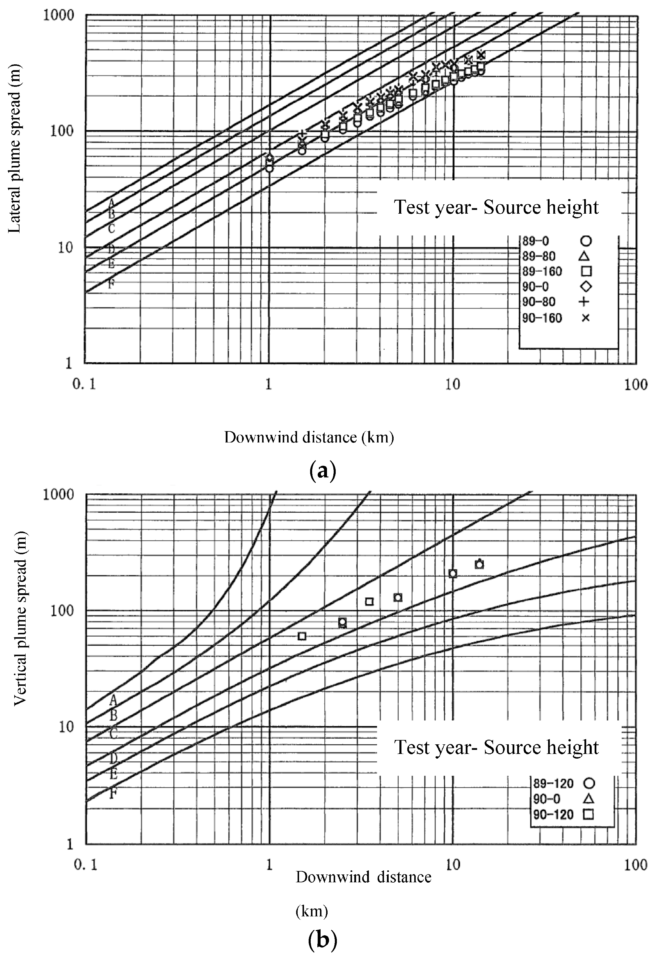
Although not the focus of this paper, it must be noted in passing that computational fluid dynamics (CFD) simulations have recently been shown to be as reliable as wind tunnel modelling in treating dispersion in the presence of site buildings (e.g., [14]). To achieve this requires high-quality CFD work and, inevitably, high-power computing resources. Ensuring quality in CFD work in general has been seen as key to the uptake of the technology in many industrial sectors; e.g., see the European Research Community on Flow, Turbulence and Combustion (ERCOFTAC) guidelines [15]. In Japan, new guidelines for using CFD simulations to obtain effective source heights at nuclear power facilities have been established by the Japan Atomic Power Society [16]. As discussed in Section 2.1, the extent of the calculations needed in nuclear safety assessment implies that CFD methods (or wind tunnel methods, for that matter) are far too computationally resource-intensive for practical applications. Assessments require a radiation dose as an end-point, and the need to treat the effects of radiation and decay in three-dimensional space makes it inevitable that final environmental assessments remain based on relatively simple Gaussian models, making use of parameters such as effective source height derived from CFD or wind tunnel simulations.

3. Field Experiment

Mt. Tsukuba is an isolated hill of 876 m (Elevation Level) near Tokyo. The field dispersion experiments were conducted by the Japan Atomic Energy Agency (JAEA) in 1989 and 1990 [4] under a wide range of meteorological conditions (wind speed, wind direction, and atmospheric stability), as shown in Table 1. Ground level concentrations were measured at 35 points within a range of 10 km from the source. The perflurocarbon (PFC) tracer gas was released from a balloon at a height of around 100 m. The release and sampling times were both 30 min. Meteorological data, including wind velocity, turbulence intensity, temperature, and solar radiation flux, were obtained at ground and upper levels. Atmospheric stability was categorized by wind speed and solar radiation flux measurements, as shown in Table 2.
Examples of concentration distributions that characterize the full set of results are shown in Figure 4, for a 30 min average time. The source point was located near the upwind foothill of Mt. Tsukuba.
Run No. 89-3 was a neutral (category D) case, and the distribution was nearly symmetrical and Gaussian. Run No. 90-5 was a stable (category F) and calm wind case, resulting in a concentration distribution that was extremely complex, with tracer gas observed in all directions around the source. High concentration appeared near the source point, due to effects of the stagnant air flow caused by the stable stratification. Run No. 90-8 was an unstable (category B) case, and the distribution was seen to be very broad. Meteorological conditions, defined by wind speed and temperature profile, varied widely over the full set of experiments. All observed data were included in the JAERI (Japan Atomic Energy Research Institute) report ([4], in Japanese). The wind tunnel experiment was conducted under the standard neutral condition recommended by the Atomic Energy Society of Japan for wind tunnel experiments in nuclear safety assessments [3].

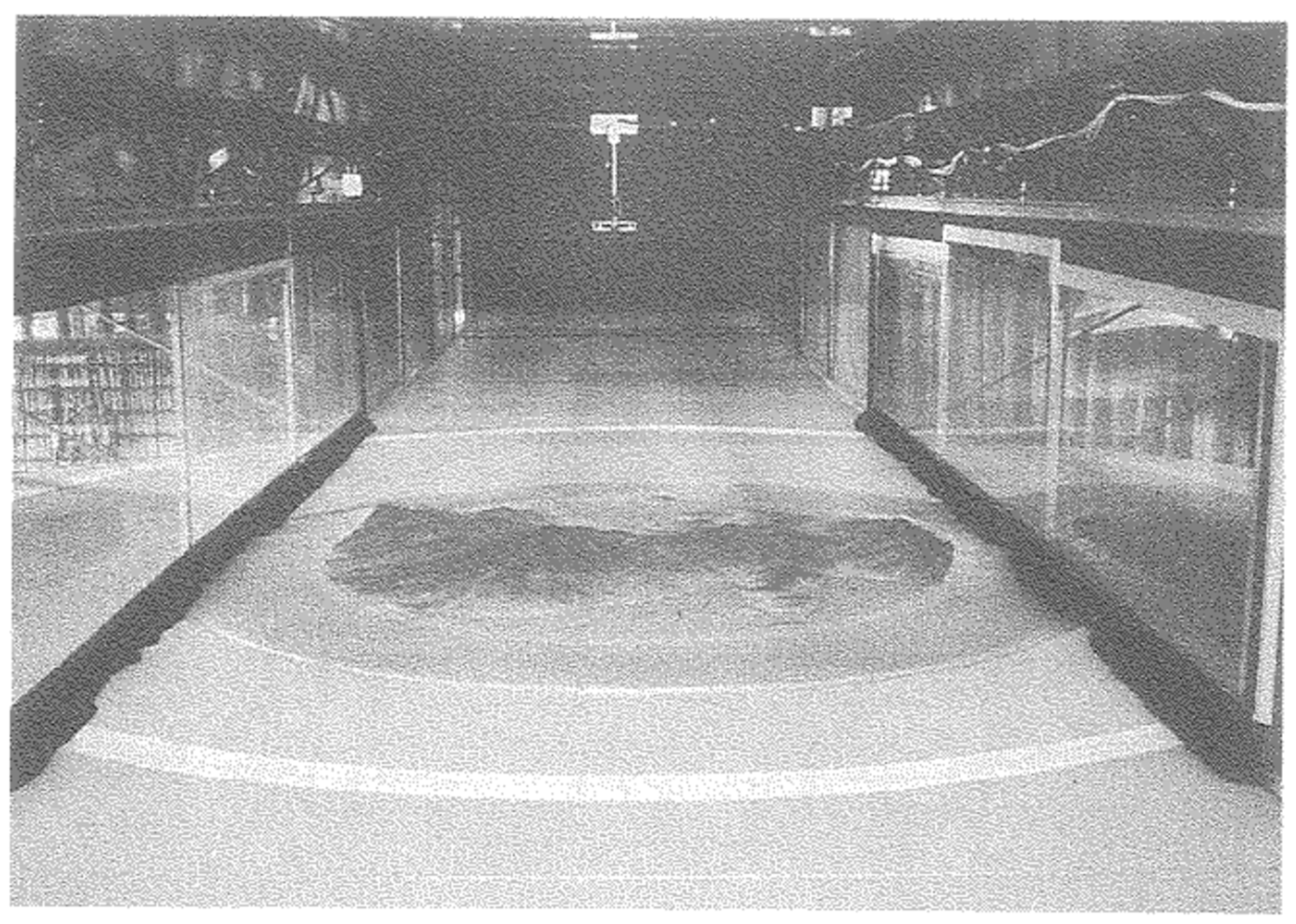
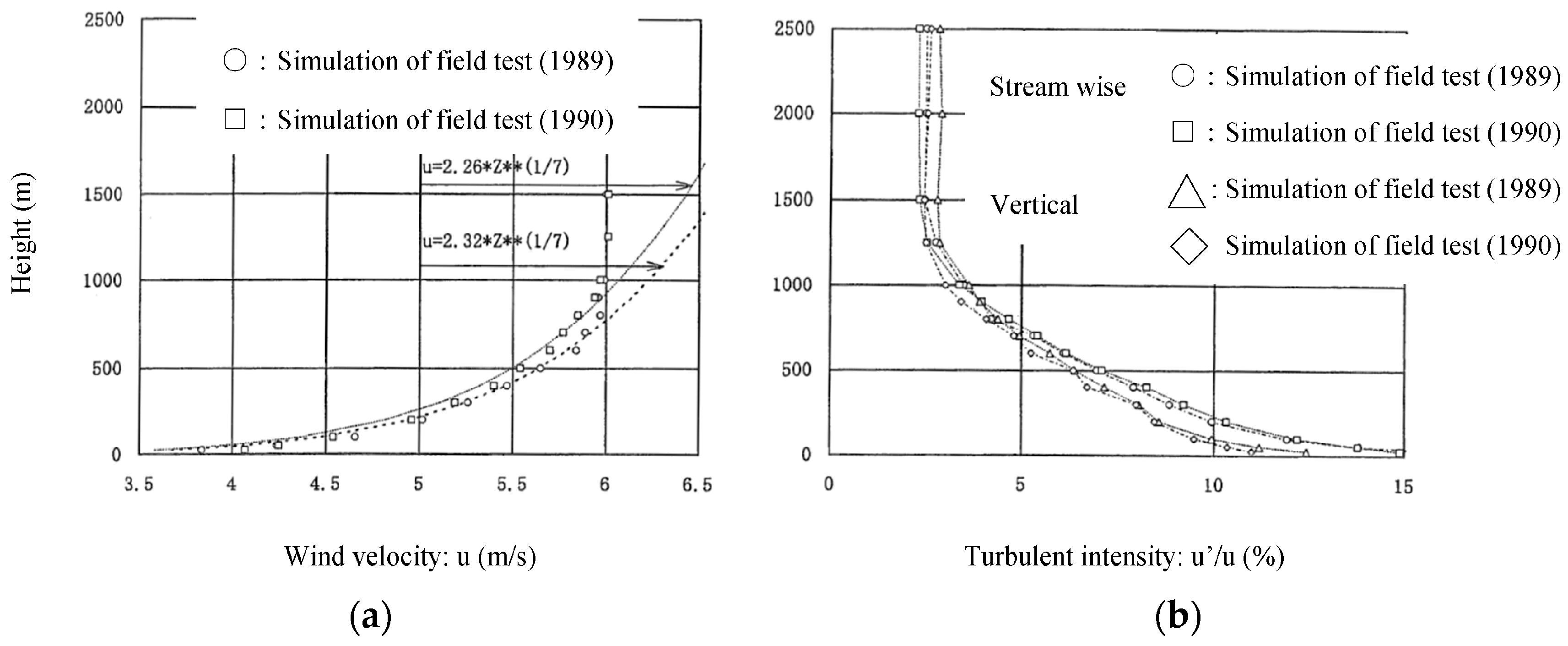
4. Wind Tunnel Experiments

The wind tunnel experiments were conducted in the year 2000 by the Japan Atomic Energy Agency, Tokai, Japan and Mitsubishi Heavy Industries Ltd., Nagasaki, Japan, using a scaled terrain model of Mt. Tsukuba, as shown in Figure 5. The outline of the experimental conditions are as follows:
  • Model scale: 1:5000
  • Wind speed: 6 m/s (free-stream), turbulence intensity: 2.5% (in upper layer), boundary layer thickness: 800 m (full scale), power law exponent: 1/7
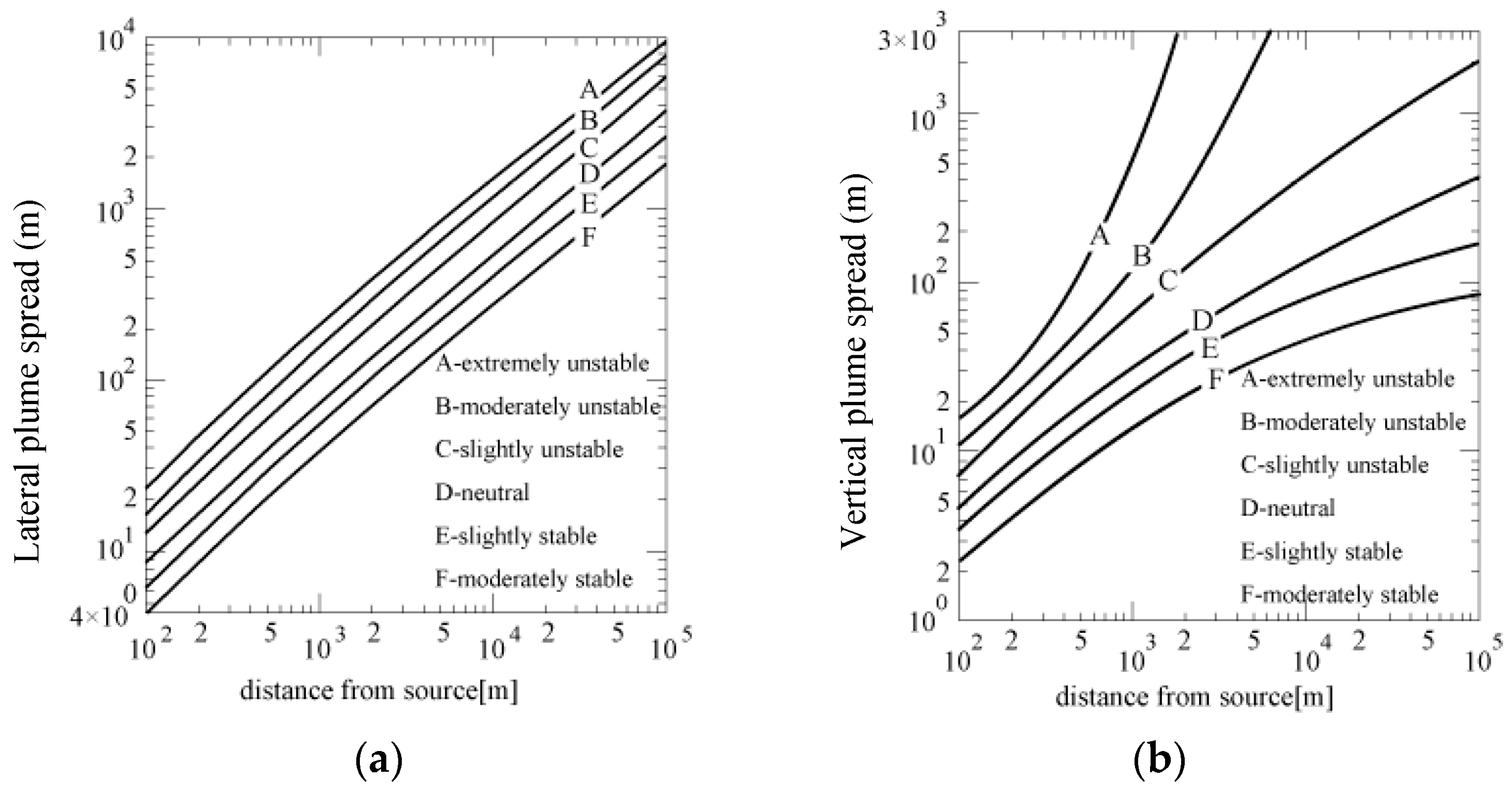
  • Plume spread without terrain: σ y (category D~F) and σ z (C~D)
  • Wind tunnel test section: 3 m width, 2 m height and 25 m length.
Wind tunnel experiments were conducted to validate the effective source height method under the same conditions of wind speed and wind direction as in the field experiment. The boundary layer profile was determined from the “Code for Wind Tunnel Experiments to Calculate the Effective Height of Emitting Source for Nuclear Power Facilities Safety Analysis” [3], not the field data. The wind tunnel profiles of wind velocity and turbulence intensity are shown in Figure 6, and the plume spread in Figure 7. Atmospheric stability conditions in the wind tunnel were neutral, i.e., there was a uniform temperature profile.
Vertical plume spread corresponds well with category C to D of neutral stability, as shown in Figure 7b, while lateral spread corresponds with category D to F. The implication is that the standard deviation of horizontal wind direction in the wind tunnel was smaller than the standard three-minute field average value associated with the Pasquill-Gifford chart.
Ground level concentration was measured at about 400 points, over a full scale range of 10 km from the source. Some examples of concentration distributions are shown in Figure 8 (solid lines), compared with the field data (dashed lines). It is apparent in Figure 8a–c that lateral plume spread in the wind tunnel is less than in the field data. This reflects differences between the fluctuations in wind direction in the wind tunnel and in the field. The mean wind direction in the wind tunnel is steady, and as a result the tracer gas distribution is narrower than in the field data. Meandering of the wind direction in the field (previously discussed in Section 2.2) is the main cause of the enhanced lateral spread. Under the stable condition of Run No. 90-5 (category F), this discrepancy becomes greater due to the additional meandering related to the stagnant regions appearing around the foothills of the mountain. It should also be noted that the field experiment returned a single realization of dispersion behavior in conditions where significant variability could be expected.
It should be noted that extensive meteorological data was observed around Mt. Tsukuba on the ground and by pilot-balloon. These does not be shown in the analysis, as the purpose of this study was to validate the use of the effective source height scheme—i.e., the end point was concentration levels. Consequently, there were no flow field measurements over the scaled model in the wind tunnel.
Previous work (e.g., [17]) has shown how the variance of the wind direction fluctuation (σθ) and the lateral plume spread (σy) in field conditions increase with the average time of the observed data, as shown in Figure 9. The original Pasquill chart [5] was compiled from field data averaged over just a few minutes. Therefore, in environmental assessments, the average time of the wind tunnel experiment and basic Gaussian plume model have been generally considered to be equivalent to 3 min. Because the average time of the field experiment at Mt. Tsukuba was 30 min, it is necessary to consider corrections based on a meandering factor M, defined in Equation (4), in order to use the wind tunnel data and Gaussian plume model together in estimating the concentration in the field. The use of the meandering factor is explained below in the Section 5.2.
M = σ θ 30 σ θ 3

5. Analysis

5.1. Terrain Effect

As already explained in the Introduction, the effective source height determined from wind tunnel experiments has been used to calculate ground level concentrations for regulatory purposes in Japan, and to a lesser degree in the U.K. In the U.K., this method has been mainly associated with the effects of complex site buildings, whereas the effects of terrain have been a focus in Japan, and this paper addresses the latter use. The aim here, therefore, is not to compare data from the wind tunnel and field directly, but to determine the validity of a calculation scheme using the effective source height, He’, in nuclear site safety assessments. The data analysis scheme is summarised in Table 3:
(1)
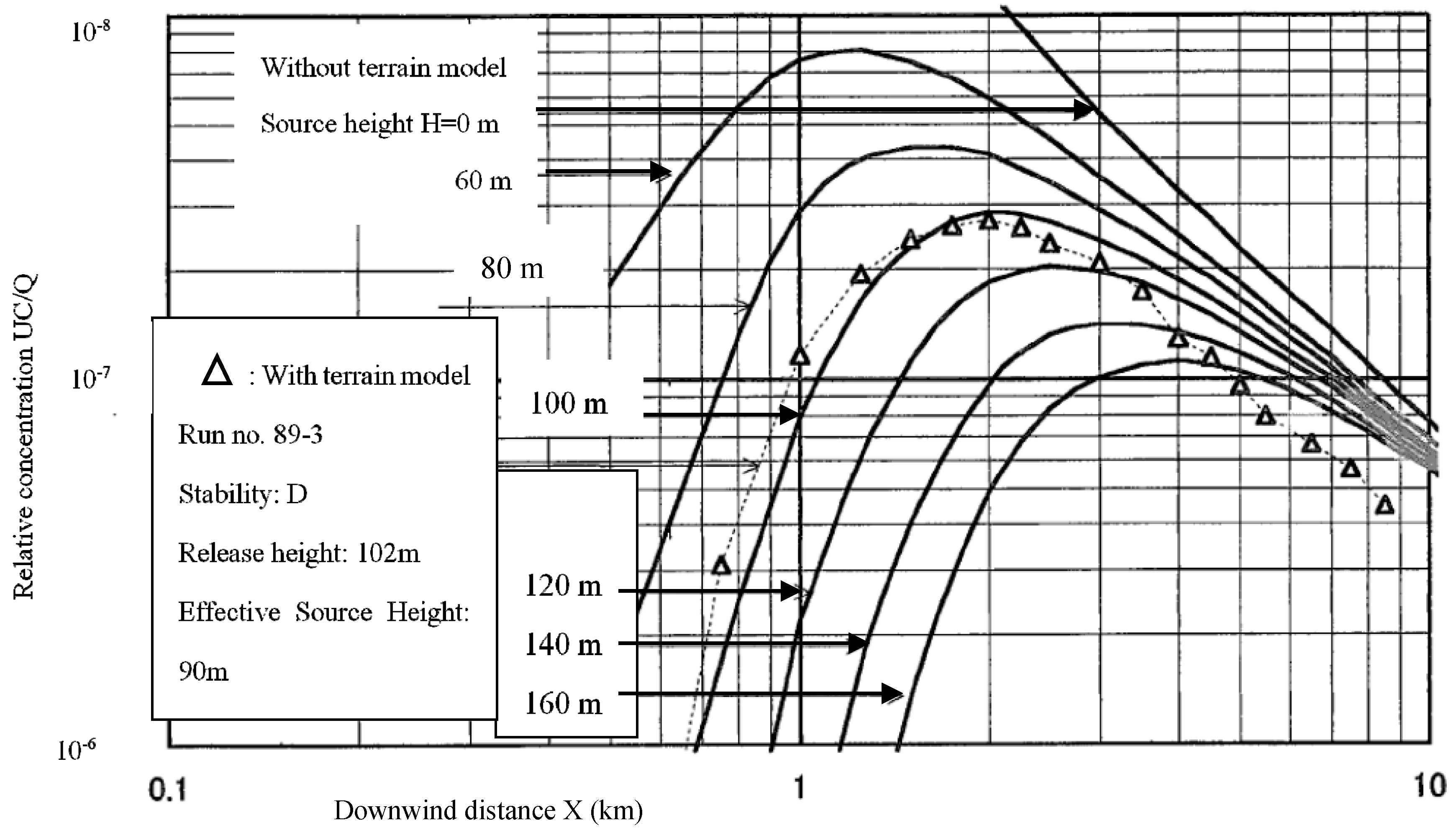
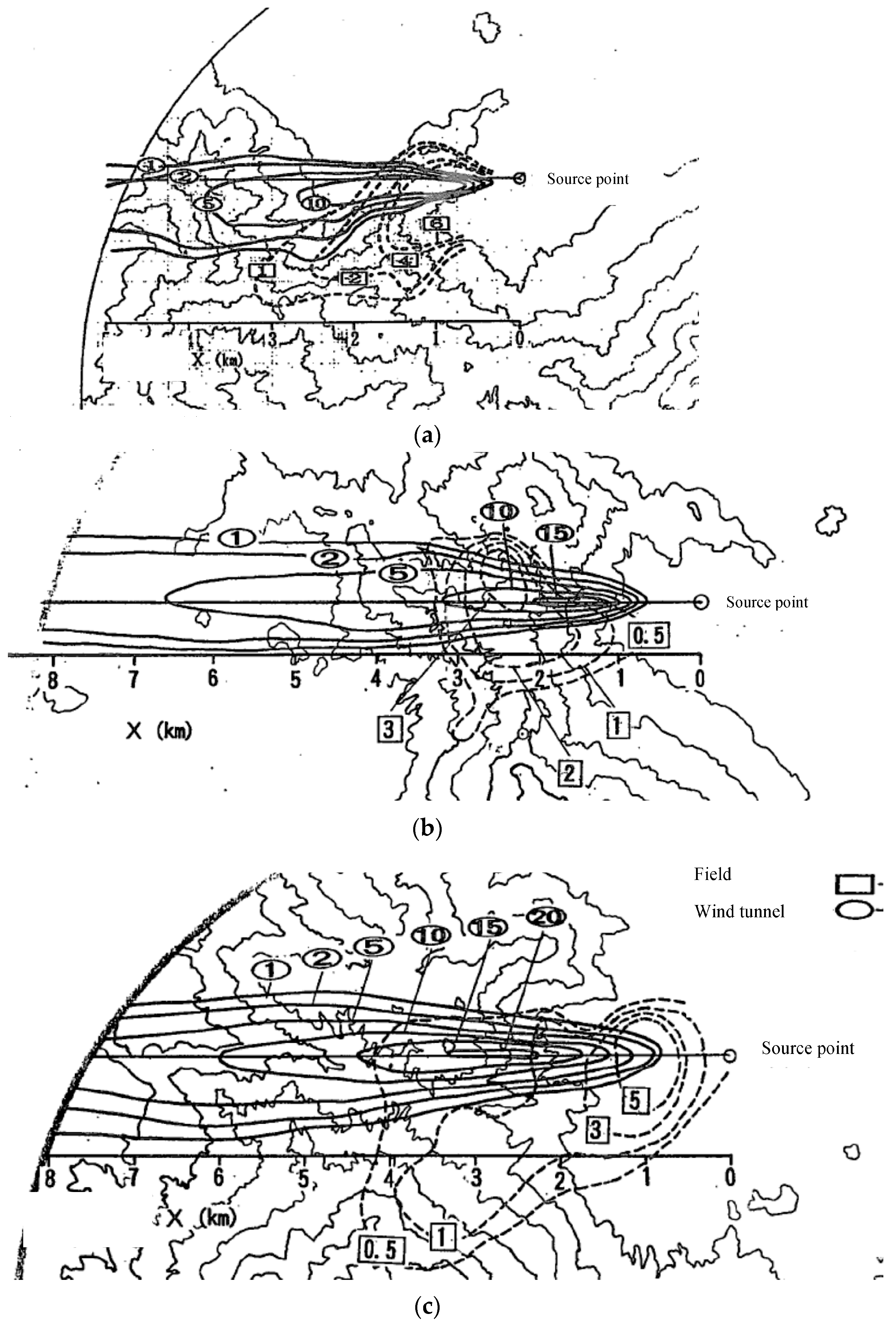
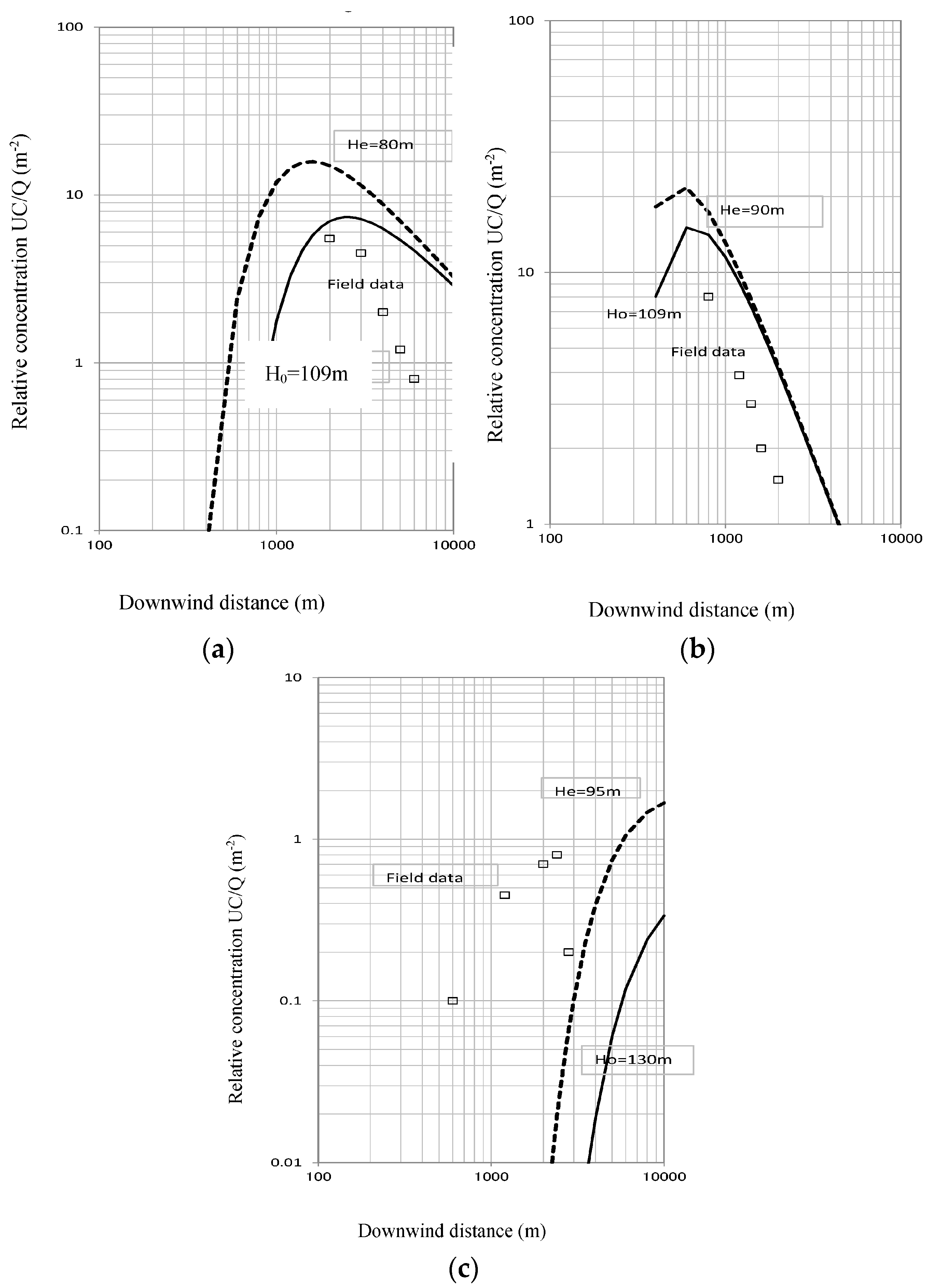
First, wind tunnel ground-level concentration data are compared between cases with and without terrain. The effective source height He’ is derived from these comparisons.
(2)
Second, calculated results using the effective source height He’ are compared with the field observation data under neutral stability.
(3)
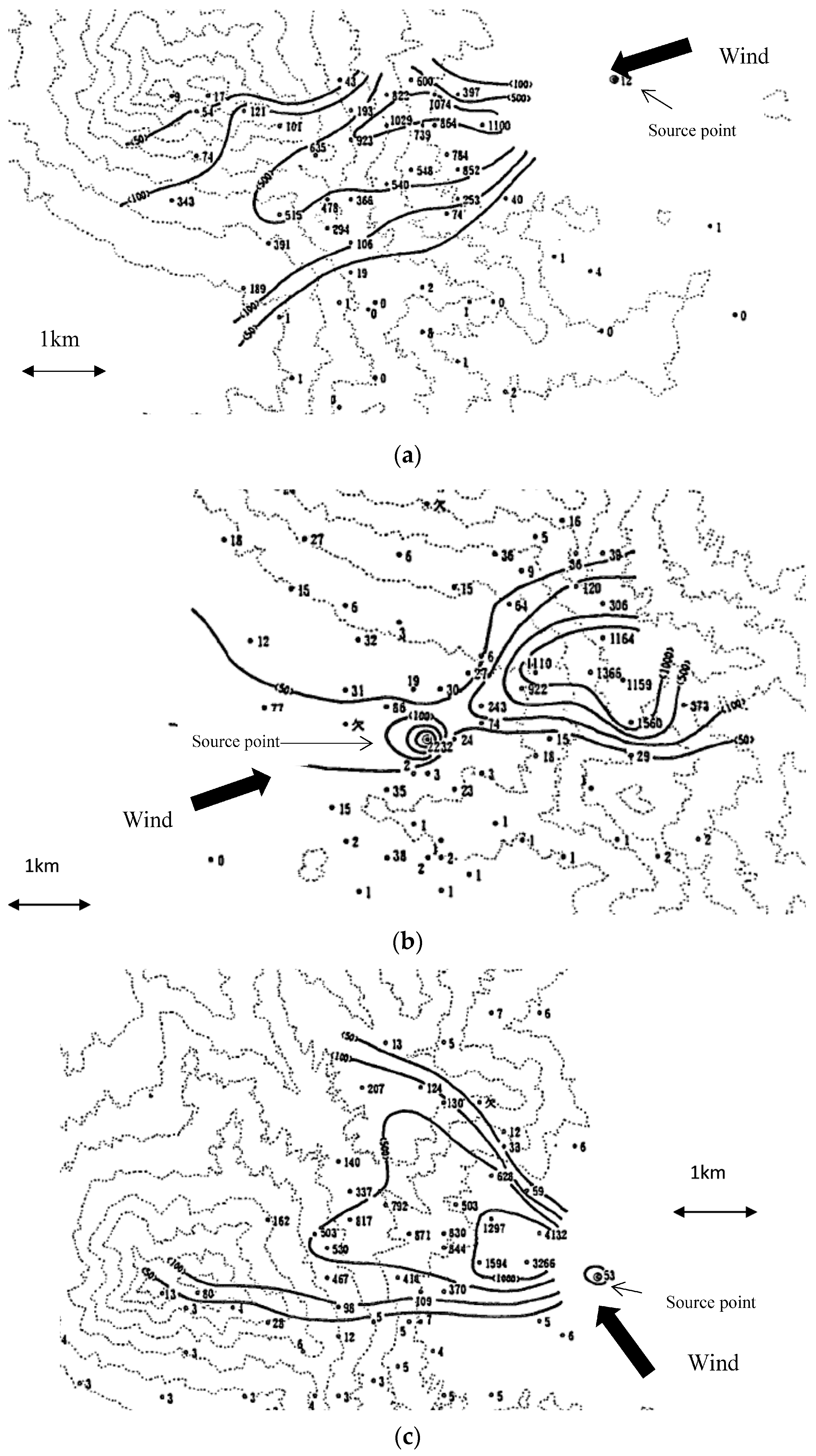
Finally, calculated results using the effective source height He’ are compared with the field observation data under non-neutral stability. The evaluation is based on comparing Result-1 and Result-2 with ground-level concentration field data measured at Mt. Tsukuba.
Results calculated with the Gaussian plume model, using the effective source height, were compared with the field data for ground-level, plume axis concentrations, as shown in Figure 10. Two calculated profiles are shown in each case: one using the effective source height He’ (dashed line), and the other the actual release height H0 (solid line).
It is apparent from Figure 10 that the calculated results using either He’ or H0 overestimate the field data, except in the case of stable atmospheric stability (category F, Run No. 90-5). A conservative estimate is a necessary condition for regulatory nuclear safety assessment purposes, and in that sense the use of either He’ or H0 would appear adequate for neutral and unstable atmospheric stabilities. The main reason for the degree of overestimation in these cases is the wind direction meandering effect discussed earlier. In the stable case, underestimation results because the model does not capture drainage flow or other stability effects over the surface of the mountain and the stagnant region near the foothills. These issues are discussed below.

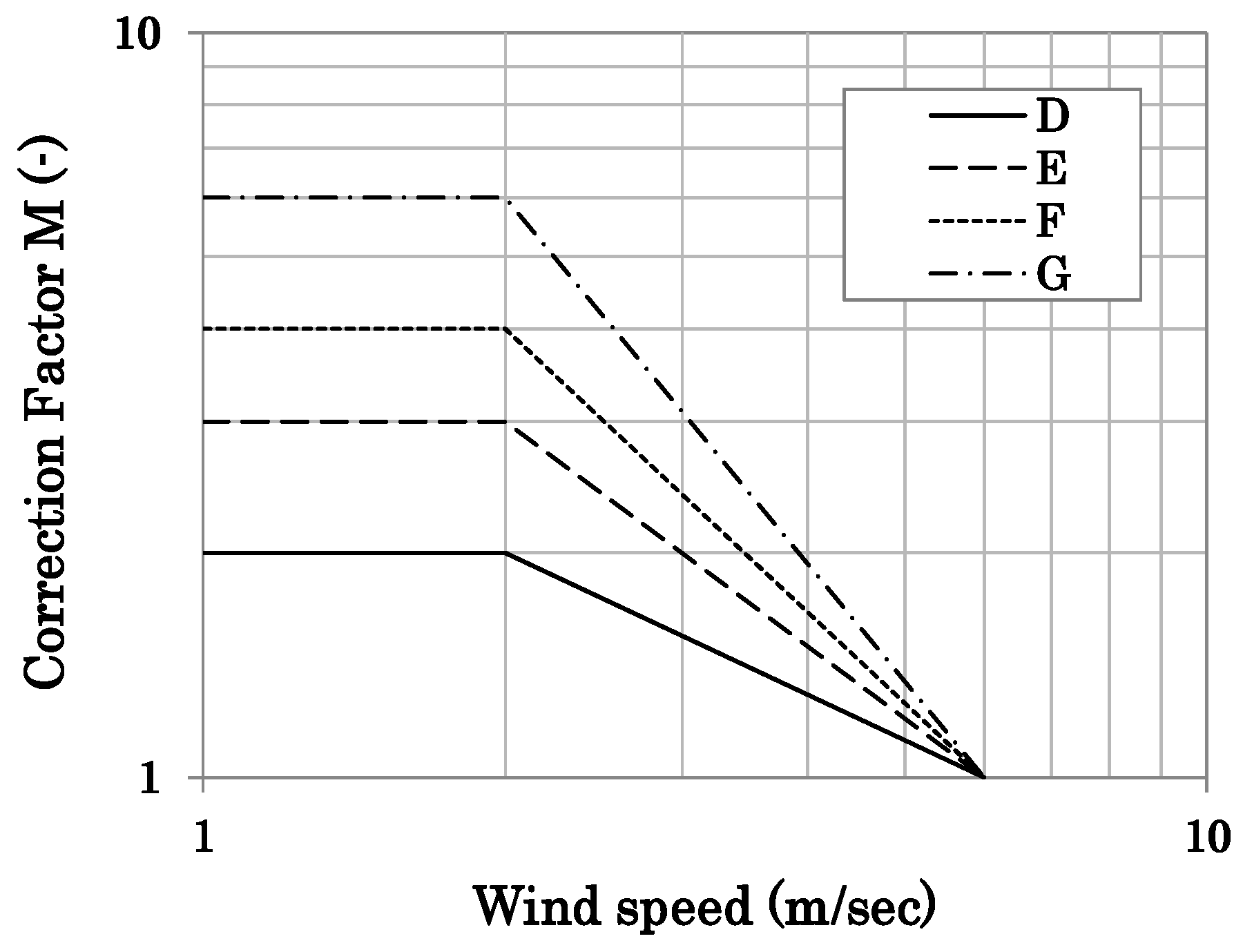
5.2. Meandering Effect

The treatment of meandering is based on the hourly-averaged field data observed by Sagendorf [18] and formulated in the U.S. Nuclear Regulatory Guide NUREG 1.145 [19] as a correction factor, M1, as shown in Figure 11. Each curve in the figure was determined from the minimum of the envelope of the observed data, and thus provides a conservative estimate of concentration. It is found from Figure 11 that the correction factor in stable conditions (categories E, F, or G) becomes larger than in neutral (category D). The correction factor for unstable conditions is very nearly 1.0, and is not actually defined in the U.S. Nuclear Regulatory Guide NUREG 1.145 [19]. It seems that the correction becomes small when turbulence diffusion is large under unstable conditions. Note that the US-NRC use the term “correction factor” instead of “meandering factor”, partly because the effects of nuclear power station buildings were included in the data. As discussed in [12,20,21], the meandering factor depends on wind velocity, stability, release height, terrain, etc. The meandering factor, M1, from the U.S. Nuclear Regulatory Guide NUREG 1.145 [19], was derived from a number of field experiments under a range of meteorological conditions at actual nuclear power stations, and has been extensively used for the nuclear safety assessment.
In the Mt. Tsukuba field experiments, the variance of wind direction was measured over the concentration sampling time (30 min.) by an ultrasonic anemometer, lifted by a balloon to the same height as the gas release, as shown in Table 1. The data were analysed to obtain the meandering factor, M2, from Equations (4) and (5); the standard 3-min average deviation of wind direction σ θ 3 was not observed, so it was calculated from the 3-min average lateral plume spread σ y 3 at 1000 m on the Pasquil chart in Figure 7. The meandering factors M2, were found to be much larger than the correction factor M1 from Figure 11, especially under stable conditions, as shown in Table 4.
M 2 = σ θ 30 σ θ 3
σ θ 3 = 180 π · σ y 3 / 1000
These factors were then used to reduce the predicted ground level concentration values, and the comparison with the data was repeated. Example results based on the resulting effective source heights are shown in Figure 12. This confirmed that:
(1)
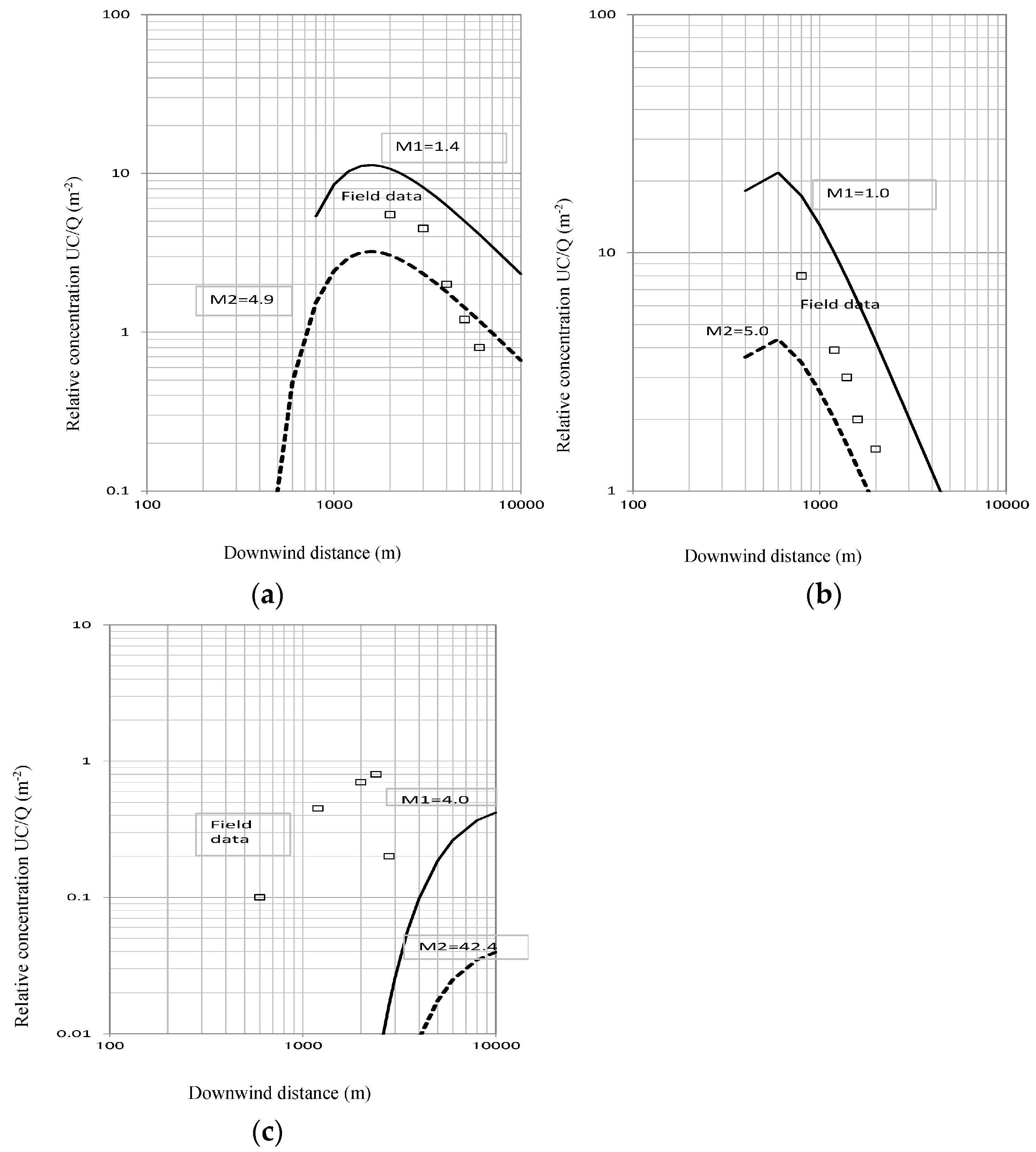
Calculated results based on the effective source height and including the meandering correction factors M1 or M2 agree reasonably well with the field data, except under stable conditions,
(2)
The results using M1 overestimate the field data (i.e., are conservative), except under stable conditions.
It can be said from these comparisons between M1 and M2 that M1 is suitable under near-neutral stability for nuclear safety assessment work, where a conservative estimation is necessary. However, it is necessary to consider the scheme to adjust the effective source height under stable conditions, like those of Run No. 90-5.

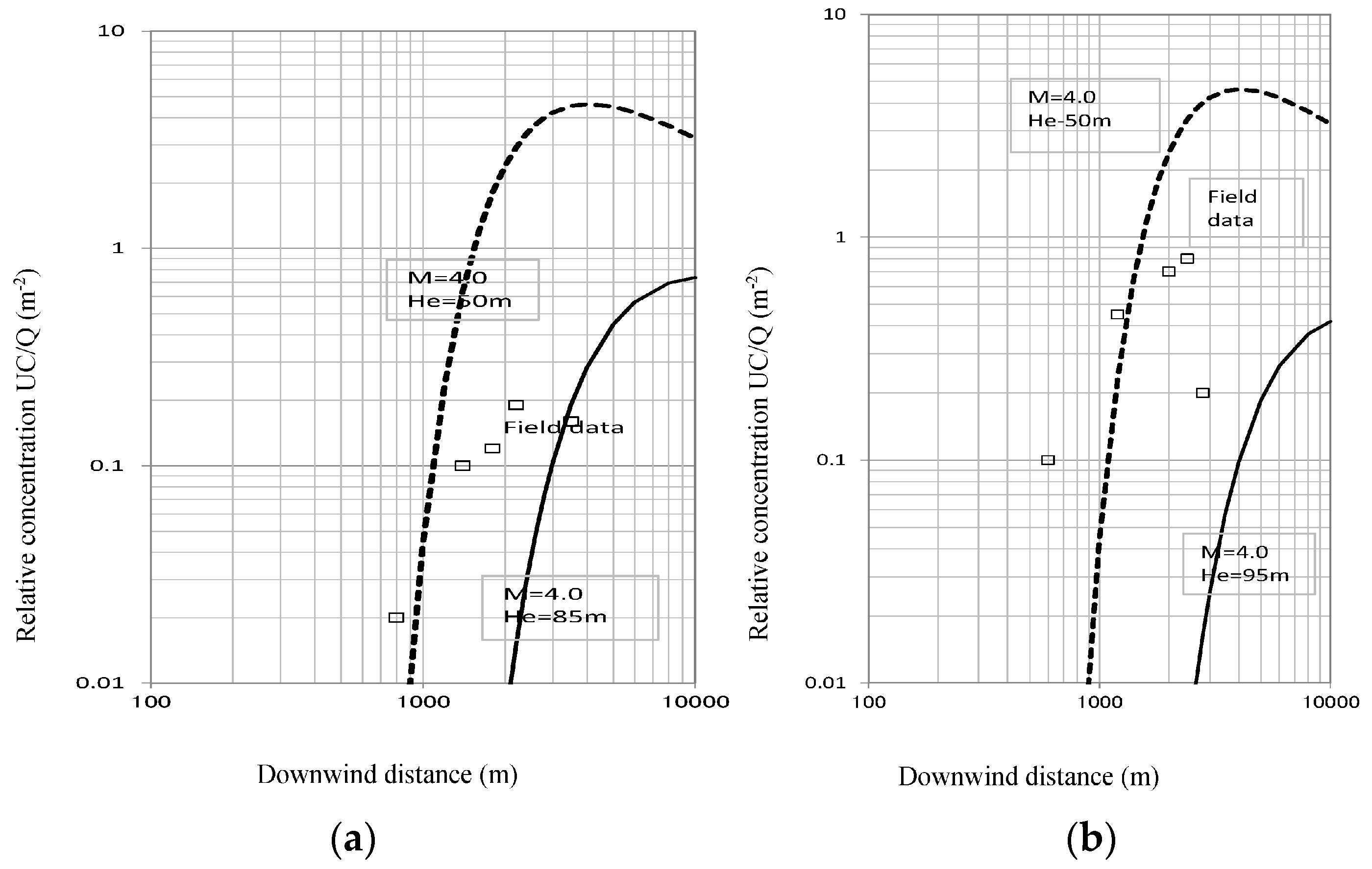
5.3. Effects of Stable Conditions

A number of special flow phenomena can arise in stable flows over terrain, particularly when winds are light [19]. As the degree of stratification increases, the vertical displacement of streamlines decreases, until they go around three dimensional terrain horizontally in very strongly stable flows around three-dimensional terrain. There is also the likelihood that, at certain critical conditions, internal wave motions can be triggered, in which case large deflections can occur, often associated with rollers (regions of recirculating flow) downwind. [22,23]. A further class of flows is associated with the downslope drainage of cool air close to the surface, termed katabatic flow. Both classes of flow can include regions of stagnant flow, upwind or downwind of the terrain. The consequences for effective source height evaluation of Gaussian plume model are clearly likely to be difficult under these stable conditions.
For example, Ohba et al. [24] conducted flow visualisation studies of plume behaviour passing over a three-dimensional hill in a thermally stratified wind tunnel. Figure 13 shows images obtained under neutral and stable stabilities. In particular, it can be seen that the height of the plume axis descends to the surface upwind, and remains low downwind of the hill due to the drainage flow in the particular stable conditions simulated.
Below, in Figure 14, we compare ground level concentrations, calculated using two effective source height options, with data observed in the field under stable conditions:
Option 1)
Effective source height = He’ (determined from neural wind tunnel experiments), meandering factor, M1 = 4.0 (determined from NUREG 1.145),
Option 2)
Effective source height = 50 m (approximately 0.5 × original source height), meandering factor, M1 = 4.0 as above.
It was found that the results calculated with Option 2 overestimated the field data beyond a downwind distance of 1 km, whereas those with Option 1 under-predicted almost all of the observations. Clearly the effective source height in these cases is closer to 50 m than the value derived for neutral conditions.
Following the Verification and Validation Standard defined by the American Society of Mechanical Engineering (ASME) [25], and considering a safety factor of two, it is recommended that a conservative estimate, such as Option 2, should be used for the assessment of nuclear plants, not Option 1.

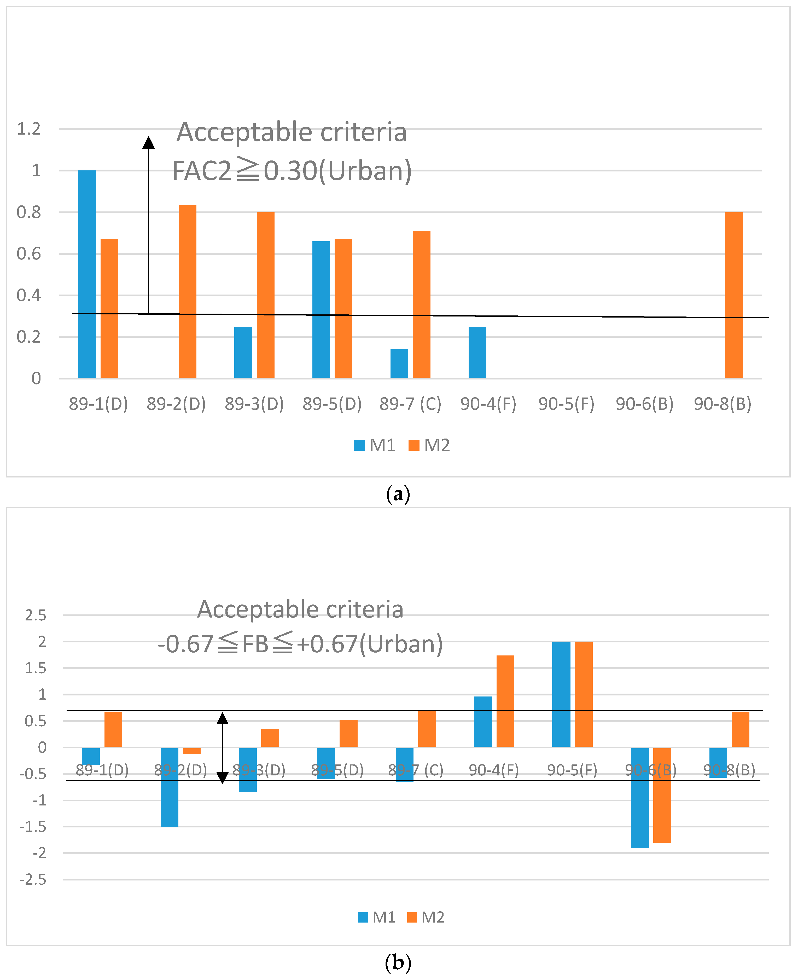
6. Acceptability Criteria

Although a conservative estimation of ground level concentrations is an important condition in nuclear safety assessment, the prediction must remain a good estimate. This can be demonstrated by testing the performance of the calculation procedures against acceptability criteria. Hanna [26] proposed a number of such criteria for the application of dispersion models in rural and urban areas, and here we apply two of these criteria, as used in the European Cooperation of Science and Technology (COST)-ES1016 research project, jointly conducted by 19 European countries [27]. The criteria are based on:
(a)
Fraction of calculated values (FAC2) (Cc) within a factor of two of observed values (Co.)
FAC2 = (fraction where 0.5 < Cc/Co < 2)
(b)
Fractional mean bias (FB)
F B = 2 ( C o C c ) ¯ / ( C o + C c ) ¯
Hanna [26] suggested the following classes of acceptability criteria from comparison studies of several atmospheric dispersion models and field data:
(a)
Rural area: Absolute value of FB ≦ 0.30, FAC2 ≧ 0.50
(b)
Urban area: Absolute value of FB ≦ 0.67, FAC2 ≧ 0.30
We argue that the Mt. Tsukuba area is similar in complexity (from a fluid mechanics point of view) to an urban area, rather than a rural area with flat terrain, and therefore applied criteria (b) for an urban area. The result of the analysis is shown in Figure 15, with calculations being based on the combined effective source height and meandering factor (M1 and M2) procedures.
Figure 15 confirms that the calculated results are close to satisfying the urban acceptability criteria of FAC2 and FB under neutral and unstable stratification conditions, but not under stable ones (Run No. 90-4 and 90-5). Use of the meandering factor M1 is desirable to ensure conservative estimation of doses in nuclear safety assessments; the FB for M1 is negative, which implies a conservative overestimation. An effective source height, equal to 50% of the actual release height, and use of the meandering factor (M1) defined by NUREG 1.145 is necessary to achieve the same end result in the special features of stable flow over Mt. Tsukuba (Run No. 90-4 and 90-5). The FB for Runs no. 90-4 and 90-5 then become conservative, with values of −1.77 and −1.27, respectively.

7. Discussion

It is concluded from the present study that
(1)
Conservative estimation of ground level concentrations under both neutral and unstable conditions can be achieved by using the effective source height He’, determined from wind tunnel experiments and the meandering factor defined by NUREG 1.145.
(2)
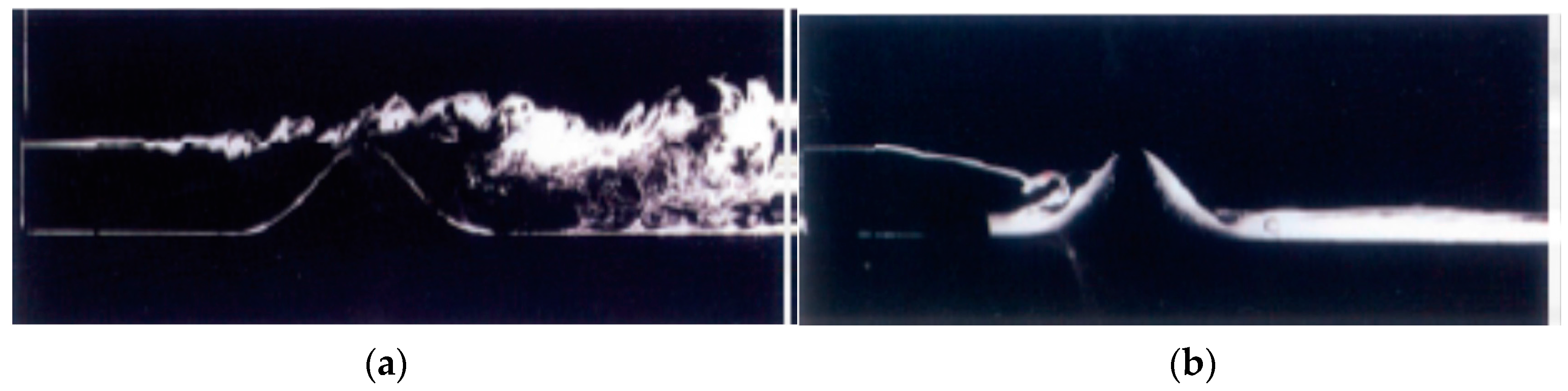
To satisfy the conservative estimate under stable conditions, a reduced effective source height is required to account for the special flow features that arise over complex terrain, such as stagnant regions and slope winds. From the viewpoint of engineering design with a safety factor of two, and following the recommendations of the ASME Verification and Validation Standard [25], use of a conservative value, such as 50% of the actual source height, is recommended.
The effective source height procedure investigated here is one of a number of adaptations of the basic Gaussian plume models to complex dispersion conditions. As here, the general intent is that resulting predictions of ground-level concentrations should be “best estimates”, yet somewhat on the conservative side—i.e., avoiding serious under-estimation. To a degree, this intent biases the performance relative to acceptability criteria. Nevertheless, the results discussed above clearly show the value of the effective source height approach to dispersion over complex terrain in windy (i.e., near-neutral) conditions. Analysis of the stable flow cases demonstrates that additional algorithms need to be introduced to represent the special flow phenomena associated with stable flow over terrain.
A wide range of phenomena is observed in stable flow over hills [23], and this will be reflected in the choice of effective stack height (i.e., each case may need to be treated on its own merits).
Finally, it should be noted that the data from the field experiment at Mt. Tsukuba were also used for the verification study of the System for Prediction of Environmental Emergency Dose Information (SPEEDI) by Chino and Ishikawa of the Japan Atomic Energy Research Institute [28].

Acknowledgments

We appreciate with the kind advices given by H. Nagai of Japan Atomic Energy Agency, S. Hanna of Harvard University, W. Snyder of the U.S. Environmental Protection Agency, and J. Sagendorf of National Oceanic and Atmospheric Administration.

Author Contributions

M. Oura conducted the fundamental calculation of dispersion model, R. Ohba analyzed the calculated wind tunnel and field data, A. Robins provided the chapter on the U.K. scheme, and S. Kato summarized all of the study.

Conflicts of Interest

The authors declare no conflict of interest.

Abbreviation

UKUnited Kingdom
NRPBNational Radiation Protection Board (UK)
ADMSAtmospheric Dispersion Modelling System
BNFLBritish Nuclear Fuels Ltd. (now Sellafield Ltd.)
CFDComputational Fluid Dynamics
ERCOFTACEuropean Research Community On Flow, Turbulence And Combustion
JAEAJapan Atomic Energy Agency
NUREGNuclear Regulatory Guide (US)
ASMEAmerican Society of Mechanical Engineering
COSTEuropean Cooperation of Science and Technology
FBFractional Bias
FAC2Factor 2

References

  1. Nuclear Safety Commission. Meteorology Guideline for Nuclear Power Facilities Safety Analysis; Nuclear Safety Commission: Tokyo, Japan, 1982. (In Japanese) [Google Scholar]
  2. Fulker, M.J.; Singh, S. The role of wind tunnel dispersion measurements in critical group dose assessments for new plant. In Air Pollution II Volume 2: Pollution Control and Monitoring; Baldasano, J.M., Brebbia, C.A., Power, H., Zannetti, P., Eds.; Computational Mechanics Publications: Southampton, UK, 1994; pp. 499–506. [Google Scholar]
  3. Atomic Energy Society of Japan. Code for Wind Tunnel Experiments to Calculate the Effective Height of Emitting Source for Nuclear Power Facilities Safety Analysis; Atomic Energy Society of Japan: Tokyo, Japan, 2009. (In Japanese)
  4. Hayashi, T.; Chino, M.; Yamazawa, H.; Nagai, H.; Moriuchi, S.; Ishikawa, H.; Adachi, T.; Kojima, H.; Okano, H.; Odagawa, H.; et al. Effective Stack Heights Obtained from Wind Tunnel and Atmospheric Diffusion Experiments; JAERI-Tech 2001-034; Japan Atomic Energy Research Institute: Ibaraki, Japan, 2001; (In Japanese). Available online: http://jolissrch-inter.tokai-sc.jaea.go.jp/pdfdata/JAERI-Tech-2001-034.pdf (accessed on 14 February 2018).
  5. Paquill, F.; Smith, F.B. Atmospheric Diffusion, 3rd ed.; Ellis Horwood Ltd.: Chichester, UK, 1983. [Google Scholar]
  6. Clarke, R.H.; National Radiological Protection Board (NRPB). The First Report of a Working Group on Atmospheric Dispersion: A Model for Short and Medium Range Dispersion of Radionuclides Released to the Atmosphere; NRPB Report R91; Atmospheric Dispersion Modelling Liaison Committee (ADMLC): Didcot, UK, 1979.
  7. Jones, J.A.; National Radiological Protection Board (NRPB). The Fifth Report of a Working Group on Atmospheric Dispersion: Models to Allow for the Effects of Coastal Sites, Plume Arise and Buildings on Dispersion of Radionuclides and Guidance on the Value of Deposition Velocity and Washout Coefficients; NRPB Report RI57; Atmospheric Dispersion Modelling Liaison Committee (ADMLC): Didcot, UK, 1983.
  8. Robins, A.G.; Macdonald, R. Review of Flow and Dispersion in the Vicinity of Groups of Buildings, Annex B, Atmospheric Dispersion Modelling Liaison Committee; Annual Report 1998/99, NRPB Report R322; Atmospheric Dispersion Modelling Liaison Committee (ADMLC): Didcot, UK, 2001.
  9. Robins, A.G.; Castro, I.P. A wind tunnel investigation of plume dispersion in the vicinity of a surface mounted cube (II): The concentration field. Atmos. Environ. 1977, 11, 299–311. [Google Scholar] [CrossRef]
  10. Robins, A.G.; Hayden, P. Dispersion from elevated sources above obstacle arrays: Modelling requirements. Int. J. Environ. Pollut. 2000, 14, 186–187. [Google Scholar] [CrossRef]
  11. Robins, A.G.; Hill, T. Borne on the Wind? Understanding the Dispersion of Power Station Emissions; Power Technology: Nottingham, UK, 2005. [Google Scholar]
  12. Hill, R.A.; Lowles, I.; Teasdale, I.; Chambers, N.; Puxley, C.; Parker, T. Comparison between field measurements of 85-Kr around the BNFL Sellafield reprocessing plant and the predictions of the NRPB R-91 and UK-ADMS atmospheric dispersion models. Int. J. Environ. Pollut. 2001, 16, 315–327. [Google Scholar] [CrossRef]
  13. Robins, A.G.; McHugh, C. Development and evaluation of the ADMS building effects module. Int. J. Environ. Pollut. 2001, 16, 161–174. [Google Scholar] [CrossRef]
  14. Hill, R.; Arnott, A.; Hayden, P.; Lawton, T.; Robins, A.; Parker, T. Evaluation of CFD model predictions of local dispersion from an area source on a complex industrial site. Int. J. Environ. Pollut. 2011, 44, 173–181. [Google Scholar] [CrossRef]
  15. European Research Community on Flow, Turbulence and Combustion (ERCOFTAC). Quality and Trust in Industrial CFD: Best Practice Guidelines, version 1.0; European Research Community on Flow, Turbulence and Combustion: Prague, Czech Republic, 2000. [Google Scholar]
  16. Atomic Energy Society of Japan. Code for Numerical Model to Calculate the Effective Height of Emitting Source for Nuclear Power Facilities Safety Analysis; Atomic Energy Society of Japan: Tokyo, Japan, 2011. (In Japanese)
  17. Ohba, R.; Ukeguchi, N.; Kakishima, S.; Lamb, B. Wind tunnel experiment of gas diffusion in stably stratified flow over a complex terrain. Atmos. Environ. 1990, 24, 1987–2001. [Google Scholar] [CrossRef]
  18. Sagendorf, J.E.; Dickson, C.R. Diffusion under Light Wind Speed in Inversion Conditions; NOAA Technical Memorandum ERL ARL-53, ARL; National Oceanic and Atmospheric Administration (NOAA): Idaho Falls, ID, USA, 1974.
  19. US-Nuclear Regulatory Commission. Atmospheric Dispersion Models for Potential Accident Consequence Assessments at Nuclear Power Plants; Regulatory Guide 1.145; US-Nuclear Regulatory Commission: Washington, DC, USA, 1979.
  20. Yee, E.; Chan, R.; Kosteniuk, P.R.; Chandler, G.M.; Biltoft, C.A.; Bowers, J.F. Incorporation of internal fluctuations in a meandering plume model of concentration fluctuations. Bound. Layer Meteorol. 1994, 67, 11–39. [Google Scholar] [CrossRef]
  21. Turner, D.B. Workbook of Atmospheric Dispersion Estimates: An Introduction to Dispersion Modelling, 2nd ed.; CRC Press LLC: New York, NY, USA, 1994; p. 179. [Google Scholar]
  22. Hunt, J.C.R.; Britter, R.E.; Puttock, J.S. Mathematical models of dispersion of air pollution around buildings and hills. In Mathematical Modelling of Turbulent Diffusion in the Environment; Harris, J., Ed.; Academic Press: London, UK, 1979; pp. 145–200. [Google Scholar]
  23. Hunt, J.C.R.; Snyder, W.H.; Lawson, R.E. Flow Structure and Turbulent Diffusion around a Three-Dimensional Hill; US EPA Report EPA-600/4-78/041; United States Environmental Protection Agency: Washington, DC, USA, 1978.
  24. Ohba, R.; Hara, T.; Nakamura, S.; Ohya, Y.; Uchida, T. Gas diffusion over an isolated hill under neutral, stable and unstable conditions. Atmos. Environ. 2002, 36, 5697–5707. [Google Scholar] [CrossRef]
  25. The American Society of Mechanical Engineers (ASME). Standard for Verification and Validation in Computational Fluid Dynamics and Heat Transfer. Available online: https://www.asme.org/shop (accessed on 23 April 2016).
  26. Hanna, S.; Chang, J. Acceptable criteria for urban dispersion model evaluation. Meteorol. Atmos. Phys. 2012, 116, 133–146. [Google Scholar] [CrossRef]
  27. COST ES1006 Best Practice Guideline. 2015. Available online: http://www.elizas.eu/index.php/documents-of-the-action (accessed on 7 January 2016).
  28. Chino, M.; Ishikawa, H. Experimental Verification Study for System for Prediction of Environmental Emergency Dose Information: SPEEDI, (III). J. Nucl. Sci. Technol. 1989, 26, 365–373. [Google Scholar] [CrossRef]
Figure 1. The Gaussian plume model, illustrating the basic concentration distribution.
Atmosphere 09 00111 g001
Figure 2. Pasquill-Gifford chart of plume spreads [5]. (a) Lateral plume spread; (b) Vertical plume spread.
Atmosphere 09 00111 g002
Figure 3. An example determination of effective source height (He’) [4].
Atmosphere 09 00111 g003
Figure 4. Contour map of 30 min averaged ground level concentrations (ppt) [4]. (a) Run No. 89-3 (D); (b) Run No. 90-5 (F); (c) Run No. 90-8 (B).
Atmosphere 09 00111 g004
Figure 5. 1:5000 scale model of Mt. Tsukuba installed in the wind tunnel [4].
Atmosphere 09 00111 g005
Figure 6. Vertical profiles of mean wind speed and turbulence in the wind tunnel flow ahead of the terrain model [4]. (a) Wind velocity (b) Turbulence intensity.
Atmosphere 09 00111 g006
Figure 7. Plume spreads over a flat terrain obtained from wind tunnel simulations [4]. (a) Lateral plume spread; (b) Vertical plume spread.
Atmosphere 09 00111 g007
Figure 8. Comparison of concentration contour maps from the wind tunnel (solid lines) and field (dashed lines) [4], where numerical values indicate normalized concentrations, UC/Q (m−2) × 106. (a) Run No. 89-3 (Neutral: D); (b) Run No. 90-5 (Stable: F); (c) Run No. 90-8 (Unstable: B).
Atmosphere 09 00111 g008
Figure 9. The dependence of the variance of wind direction on average time [17].
Atmosphere 09 00111 g009
Figure 10. Plume axis concentration distribution for each atmospheric stability. Predictions with actual source height (solid line); effective source height (dashed line). (a) Run No. 89-3 (neutral: D); (b) Run No. 90-8 (unstable: B); (c) Run No. 90-5 (stable: F).
Atmosphere 09 00111 g010
Figure 11. Correction factor, M1, defined by the U.S. Nuclear Regulatory Guide (NUREG) 1.145 [19].
Atmosphere 09 00111 g011
Figure 12. Comparison of the field data with the model predictions, based on the effective stack height, and including corrections for meandering (i.e., using M1, solid line, or M2, dashed line). (a) Run No. 89-3 (D); (b) Run No. 90-8 (B); (c) Run No. 90-5 (F).
Atmosphere 09 00111 g012
Figure 13. Images of gas dispersion around a hill in a thermally stratified wind tunnel (flow is from left to right). (a) Neutral stability; (b) Stable stability.
Atmosphere 09 00111 g013
Figure 14. Comparison of calculated concentrations with field data under stable conditions (category F); option 1 is represented by a solid line, option 2 by a dashed line. (a) Run No. 90-4 (F); (b) Run No. 90-5 (F).
Atmosphere 09 00111 g014
Figure 15. Comparison of calculated results with acceptability criteria, where no bar at a run number means zero. (a) Factor 2 (FAC2); (b) Fractional mean bias (FB).
Atmosphere 09 00111 g015
Table 1. Experimental conditions for the gas release and meteorology corresponding to the near-neutral and the non-neutral stabilities in the field experiments [4].
Run No.Experimental Condition for the Gas Release and Meteorology Corresponding to
Near-Neutral Stability in the Field Experimentsthe Non-Neutral Stability in the Field Experiments
89-189-289-389-589-790-490-590-690-8
Year/Month/date14 November 198915 November 198915 November 198917 November 198920 November 198911 November 199012 November 199013 November 199015 November 1990
Sampling time (Japanese standard time)14:00–14:3011:00–11:3015:30–16:0012:00–123015:30–16:0021:00–21:3020:00–20:3014:30–15:0012:00–12:30
Release height (m)1168910290119102130107109
Wind speed (m/s)4.55.24.53.03.61.50.12.32.0
Wind direction (deg.)98697647323324239149134
Atmospheric stabilityDDDDCFFBB
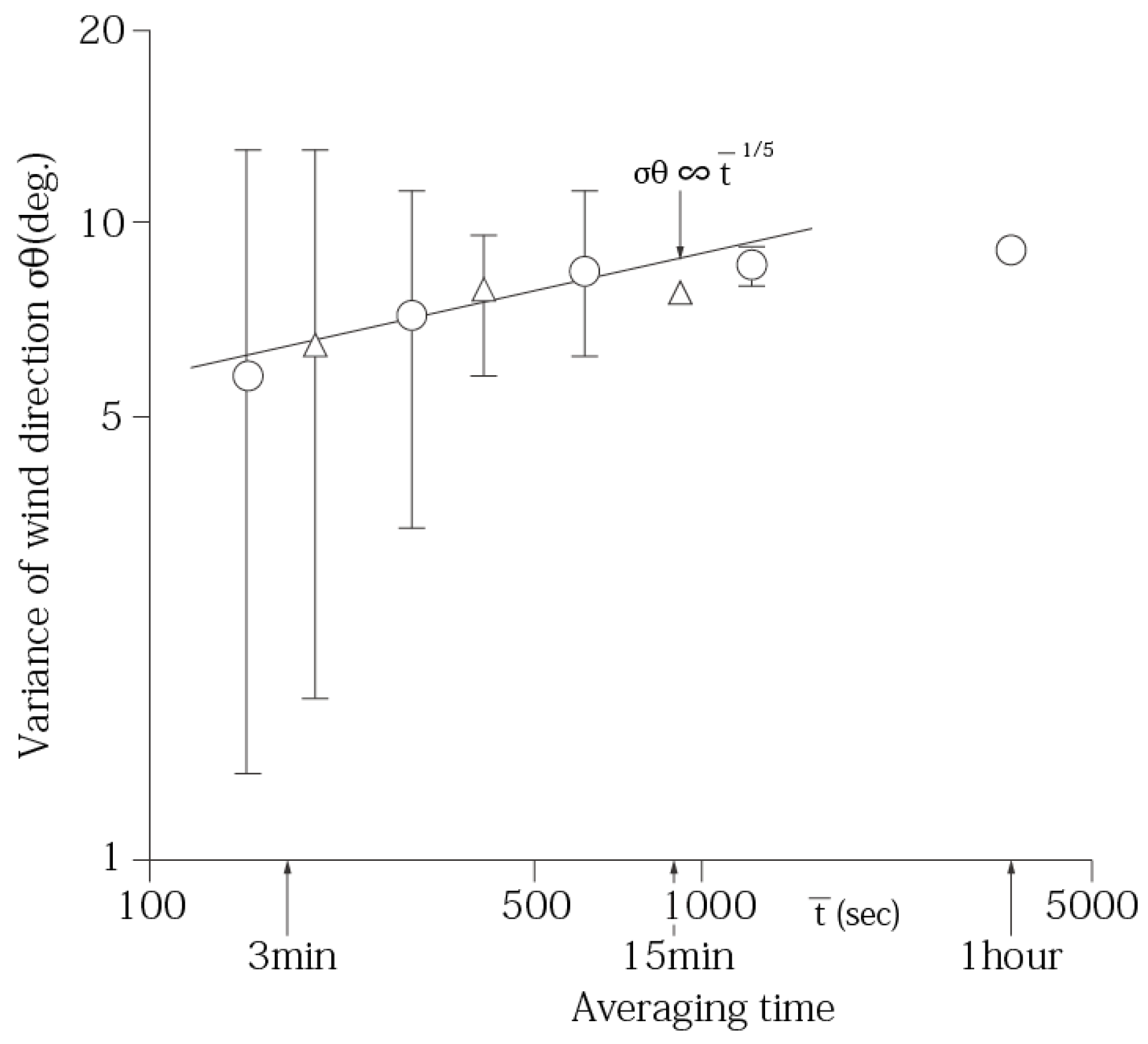
Fluctuation of wind direction (deg.) for sampling time (30 min)16.628.821.037.125.145.392.727.943.1
Table 2. Categorization of atmospheric stability [5].
Wind Speed (m/s)Radiation Flux in Daytime (kw/m2)Radiation Flux in Nighttime (kw/m2)
>0.600.30 ~ 0.600.15 ~ 0.300.15>−0.02>−0.04 ~ −0.02−0.04>
<2ABBDDFF
2~3BBCDDEF
3~4BCCDDDE
4~6CDDDDDD
6<CDDDDDD
Table 3. Schematic representation of the calculation scheme for nuclear safety assessment.
ToolsWithout TerrainWith Terrain
NeutralNon-NeutralNeutralNon-Neutral
Wind tunnel experimentWind Tunnel-1Wind Tunnel-2
Atmosphere 09 00111 i001
He’
Calculation of Gaussian plume model Atmosphere 09 00111 i002Result-2
Result-1
Table 4. Correction factors M2 used for the calculation of concentrations.
Run No.StabilityLateral Plume Spread (m)Meandering Factor (M2)Correction Factor (M1)
σy3σy30σθ30
89-1D76.3299.516.63.91.4
89-2D76.3508.228.86.71.2
89-3D76.3374.221.04.91.4
89-5D76.3651.737.18.51.75
89-7C104.9450.225.14.31.0
90-4F38.1791.245.320.74.0
90-5F38.11617.592.742.44.0
90-6B152.6510.027.93.31.0
90-8B152.6767.243.15.01.0

