Impacts of Traffic Tidal Flow on Pollutant Dispersion in a Non-Uniform Urban Street Canyon
by
Tingzhen Ming
1, 
Weijie Fang
1,
Chong Peng
2,*,
Cunjin Cai
1,
Renaud De Richter
3,
Mohammad Hossein Ahmadi
4 and
Yuangao Wen
1 1
School of Civil Engineering and Architecture, Wuhan University of Technology, No. 122 Luoshi Road, Hongshan District, Wuhan 430070, China
2
School of Architecture and Urban Planning, Huazhong University of Science and Technology, No. 1037, Luoyu Road, Hongshan District, Wuhan 430074, China
3
Tour-Solaire.Fr, 8 Impasse des Papillons, F34090 Montpellier, France
4
Faculty of Mechanical Engineering, Shahrood University of Technology, Shahrood 3619995161, Iran
*
Author to whom correspondence should be addressed.
Atmosphere 2018, 9(3), 82; https://doi.org/10.3390/atmos9030082
Submission received: 5 January 2018
/
Revised: 13 February 2018
/
Accepted: 22 February 2018
/
Published: 25 February 2018
(This article belongs to the Special Issue Recent Advances in Urban Ventilation Assessment and Flow Modelling)
Abstract
:A three-dimensional geometrical model was established based on a section of street canyons in the 2nd Ring Road of Wuhan, China, and a mathematical model describing the fluid flow and pollutant dispersion characteristics in the street canyon was developed. The effect of traffic tidal flow was investigated based on the measurement results of the passing vehicles as the pollution source of the CFD method and on the spatial distribution of pollutants under various ambient crosswinds. Numerical investigation results indicated that: (i) in this three-dimensional asymmetrical shallow street canyon, if the pollution source followed a non-uniform distribution due to the traffic tidal flow and the wind flow was perpendicular to the street, a leeward side source intensity stronger than the windward side intensity would cause an expansion of the pollution space even if the total source in the street is equal. When the ambient wind speed is 3 m/s, the pollutant source intensity near the leeward side that is stronger than that near the windward side (R = 2, R = 3, and R = 5) leads to an increased average concentration of CO at pedestrian breathing height by 26%, 37%, and 41%, respectively. (R is the ratio parameter of the left side pollution source and the right side pollution source); (ii) However, this feature will become less significant with increasing wind speeds and changes of wind direction; (iii) the pollution source intensity exerted a decisive influence on the pollutant level in the street canyon. With the decrease of the pollution source intensity, the pollutant concentration decreased proportionally.
1. Introduction
The recent urbanization process continues to advance all over the world. The rapid growth of vehicle ownership leads to motor vehicle exhaust emissions being one of the main sources of air pollution in cities [1]. Streets become increasingly canyon-style in modern cities due to the increasing frequency of tall buildings. Traffic growth and related congestion results in increased pollution emissions. The construction of high-rise buildings and the increase of building density have caused the deterioration of the urban ventilation environment. Consequently, the pollutants emitted from vehicles are difficult to be diluted and disperse slowly. These factors severely endanger travelers who are directly exposed to the atmosphere and this furthermore has a severe impact on the indoor air quality of street buildings.
Environmental pollution is a severe problem, threatening the health and survival of human beings [2,3,4]. Primarily due to these health-related issues, extensive research on identifying and understanding the physical processes that both drive and influence the near-field pollutant dispersion in urban environments has experienced a substantial progress over the last three decades. Most of these studies began with the basic unit of any city—the Street Canyon. This has been defined as a relatively narrow street space formed by successive buildings on both sides of a city street [5]. Relevant studies mainly relied on field measurements [6,7], wind tunnel experiments [8,9,10], and numerical simulations [11,12,13]. Based on previous studies, important factors that influence the flow patterns and the dispersion mechanism of pollutant can be grouped into the following categories: Inflow conditions (such as wind speed, wind direction [14,15,16], turbulence intensity [17]); Geometric conditions of building structures (such as building aspect ratio [18,19] and the street canyon aspect ratio [20,21]); Ground surface and building surface conditions (such as building surface roughness and hot or cold conditions [22,23,24,25]); The impact of turbulences caused by vehicle movement [11]. Although the research results in this field are substantial and mature, Lateb et al. [26] clearly concluded that “the topic of micro-scale dispersion still requires further investigation to understand the effect of all parameters on wind flow and pollutant dispersion in urban areas”.
At present, both in large and medium-sized cities, by the influence of urban planning layout and the increasing price of central area land, a new pattern of work unit has formed that focuses on the city center area, while the residential areas are mainly concentrated in peripheral regions. In the morning, a large number of motorized vehicles enters the city on one side of the roads, while in the afternoon, a similar number of motorized vehicles leaves the city on the other side of the roads. Usually, this phenomenon is called traffic tidal flow as shown in Figure 1. Traffic tidal flow will increase the pollution source on one side of the road than on the other side because the motor vehicles on one side of the road are far more numerous than on the other side. However, most previous studies on the definition of pollution source are too idealistic, often assuming the pollutant emission source as the constant point source or line source in the center of the road. In addition, geometric models often assume an ideal canyon type with a uniform building roof height. Using even and uneven roof height along each courtyard building’s wall of a regular urban array, Nosek et al. [27] showed that the pollutant fluxes and pollutant removal capabilities through the street-canyon roof top are strongly affected by the roof-height arrangement. Gu et al. [28] furthermore highlighted that the roof-height non-uniformities along both street-canyon walls are able to either improve or worsen the air quality of the street-canyon with regard to the source position and above-roof wind direction. Recently, Nosek et al. [29] employed two street canyon models with either uniform building roof height or non-uniform building roof height to analyze the dispersion characteristics of pollutants. The results showed that the buildings’ roof-height variability at the intersections plays an important role for the resulting dispersion of traffic pollutants within the canyons. These studies provided insight into the pollutant dispersion within street networks formed by blocks of non-uniform height. Therefore, our study focused on the impact of traffic tidal flow on pollutant dispersion in a non-uniform urban street canyon.
The present study is principally an extension of the study of urban traffic pollution and the aims are as follows: (i) to investigate the pollutant exchange processes in a 3D asymmetrical street canyon; (ii) to analyze the impacts of traffic tidal flow on pollutant concentration distribution characteristics; (iii) to find the correlations between source intensity and pollutant concentration levels in the street space. The pollution was simulated via homogeneously emitted passive gas (CO) from a ground-level volume source. Both volume sources were positioned along the two traffic-ways of the investigated street canyon. Field measurements of the traffic flow in two parallel traffic-ways at different time intervals (6:00 a.m. to 8:00 p.m.) were conducted and the results formed the pollution source intensity of the Computational Fluid Dynamics (CFD) method.
2. Model Description
2.1. Geometric Model
A three-dimensional geometrical model was established based on a section of the street canyon in the 2nd Ring Road of Wuhan, China, as an apparent traffic tidal phenomenon regularly occurs in this road. The street length is 220 m. There are six standard motorways in the middle of the road (three on each side) and the width of each lane is 4 m. Either side of the motorway has a non-motorized lane with a single width of 5 m. The total width of the street is 34 m. Street buildings are four main middle-rise residential buildings and a large number of low-rise shops. Not only is this particular road very busy, there are also many pedestrians on both sides of the street. Following appropriate simplification principles we built the geometric model using the Gambit 2.4.6 software (FLUENT INC., Lebanon, NH, USA). Considering the non-uniform distribution of the pollution source under the influence of traffic tidal flow, two pollution sources were set up. The three motorways on the left side became source 1 and those on the right became source 2. This was the main difference to previous studies.
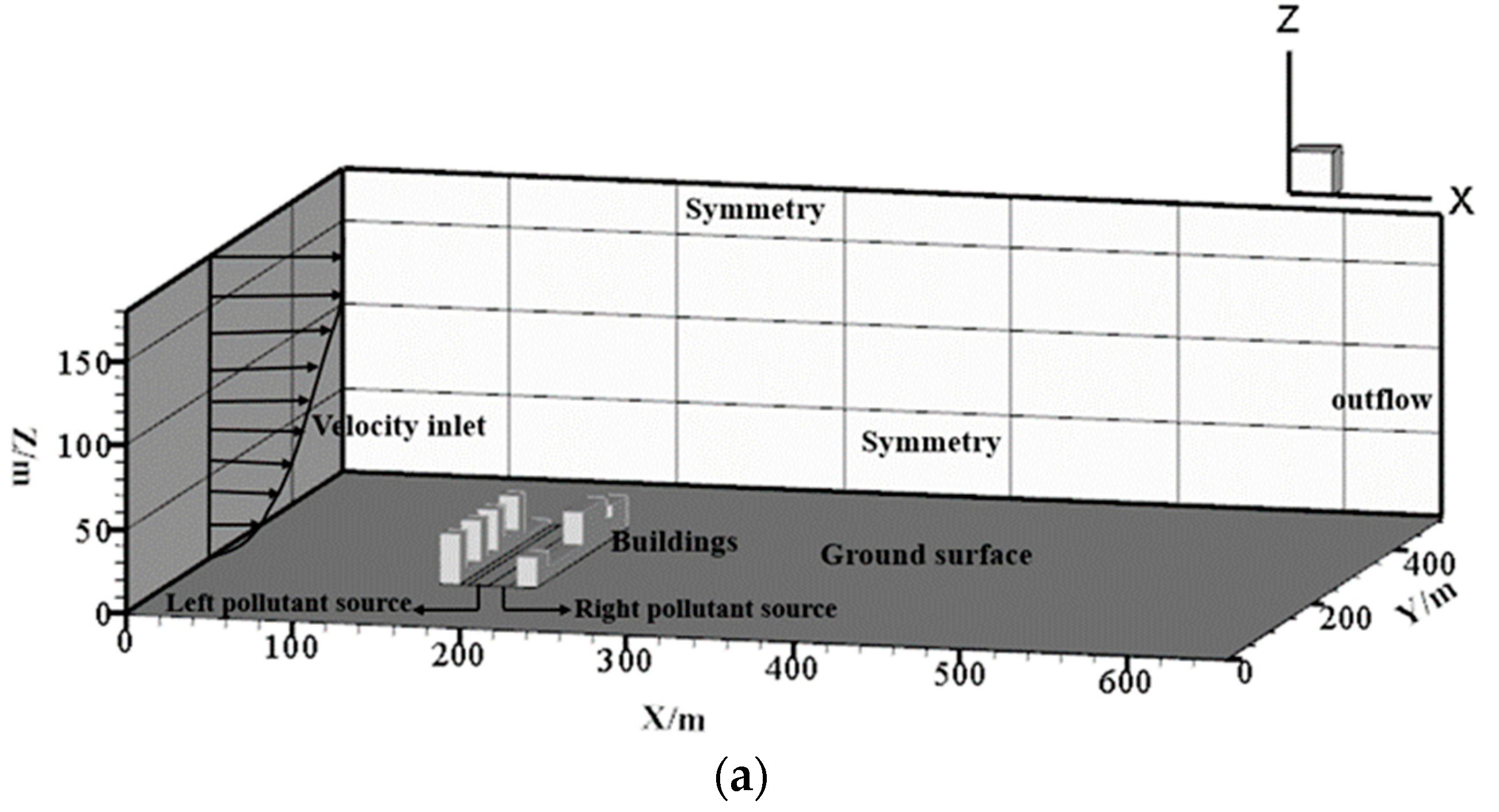
The maximum height of the street buildings was 30 m. Because the maximum height of the buildings (30 m) on both sides of the road still remained below the street width (34 m), the canyon type belonged to the shallow street canyon, where the wind blows easily to the bottom of the street. According to the technical guidance of the Japan AIJ building outdoor wind environment CFD simulation [30], the computing area inlet met 5 H from the windward building boundary, and the lateral boundary was 5 H from the edge of the building. The top boundary was set to be 6 H from the ground, and the outlet boundary was located 15 H from the leeward building edge. H was the target height. This study used H = 30 m as the maximum height. The area of the building covered less than 3% of the total computing area. Based on the above principles, the total size of the computing domain X × Y × Z was 658 m × 520 m × 180 m. The computing domain model and the boundary conditions are shown in Figure 2 below.
2.2. Mathematical Model
Pollutant dispersion in built environments is a both central and complex issue. Complex flow patterns control the wind flow around the buildings; therefore, the dispersion of pollutants in a street canyon is a typical turbulence dispersion issue [31,32]. Consequently, the choice of an accurate CFD turbulence model is a prerequisite for calculation accuracy.
At present, the Reynolds-averaged Navier–Stokes (RANS) turbulence model is widely used for numerical simulations of street canyons. Many scholars have compared different RANS models [33,34,35]. The standard k-ε model (SKE) is less able to show separation flow because it overestimates the turbulence kinetic energy near the windward corner of buildings. In addition, when there is a source exit in the recirculation area of roof and wall, the concentration can be predicted to be low. The renormalization group k-ε (RNG) turbulence model is a modification of the standard k-ε model, which performs well in the prediction of pollutant concentration [36]. Compared to the LES model that has been favored by scholars in recent years, the resulting simulation results show a good agreement [37]. The RNG k-ε model has been widely used to simulate the complex flow of air in construction groups or urban areas [38,39,40]. Therefore, to guarantee calculation accuracy and to ensure that computer resources remain as small as possible, this study employed the RNG k-ε turbulence model proposed by Yakhot and Orszag [41] to simulate the influence of turbulence. The flow of viscous incompressible fluids is commonly described with the Navier-Stokes equations [15]. The solution control equations are as follows:
- Continuity Equation:
- Momentum conservation Equation (N-S):
- Turbulence kinetic Equation k:
- Turbulent kinetic energy dissipation rate ε:
In the above Equation, Ui and Uj represent the average velocity components in the i and j direction coordinates, respectively; represents the air density and P represents the air pressure; ν represents the kinematic viscosity; represents the Reynolds stress term; represents the Kronecker function; k and ε represent the turbulent kinetic energy and turbulent dissipation rate, respectively; G represents the production of turbulent kinetic energy due to the average velocity gradient. represents the turbulence eddy viscosity. Cμ, Cε1 and Cε2 represent empirical constants which can be assumed to be 0.09, 1.44, and 1.92, respectively; and represent the turbulent Prandtl numbers corresponding to the turbulent kinetic energy and the turbulent dissipation rate, respectively, which can be assumed to be 1.0 and 1.3, respectively. , = 0.012, = 4.38 [42].
The species (pollutant) transport Equation:
represents the pollutant concentration (kg/m3), represents the pollutant emission rate (kg/m3 s). represents the turbulent eddy diffusivity of pollutants. Here , represents the turbulent eddy viscosity, represents the turbulent Schmidt number, which represents the ratio of momentum diffusivity and mass (or pollutants) diffusivity. Here we use = 0.7 according to Hang et al. [43].
2.3. Boundary Conditions
2.3.1. Inlet Boundary
The vertical characteristics of the wind speed are affected by terrain and have a close relationship with the roughness of the terrain. Due to the roughness of the ground, wind flow often occurs in the form of gradient winds (see Figure 2). For the inlet boundary conditions, either the exponential law or the logarithmic law can be used as an expression of the wind velocity profile [44,45]. As a result, this paper employed the exponential law for the wind speed profile expression:
where represents the average wind speed at the reference altitude and represents the ground roughness index. The reference height is usually 10 m above the ground. When increases beyond a certain height , different ground conditions lead to different ground roughness index value. According to Wang et al. [46], the simulation value of was chosen to be 0.22.
The inlet boundary turbulence is also an important factor affecting flow characteristics. The following expression describes the turbulent kinetic energy and the dissipation rate at the inlet boundary:
where represents the friction velocity, which is the square root of the ratio of turbulent shear stress to air density. refers to the von Karman constant 0.4; here, the value of was 0.09.
For this study, wind speeds of 1.5 m/s, 3 m/s, 4.5 m/s, and 6 m/s at the reference height of 10 m and wind directions of 0°, 30°, 45°, 60° and 90° were employed.
2.3.2. Outlet Boundary
After taking the effects of ambient wind into account, two vertical surfaces in the model can be considered as outlet boundary, upper and right borders, respectively. To avoid the influence of the “reflection source” formed by the pressure boundary on the calculation convergence, the right exit uses a free flow boundary; however, the upper boundary had a relatively static pressure of zero; therefore, the boundary of the symmetry plane was used.
2.3.3. Lateral Boundary
The two sides and the top of the domain were far away from the building wall, and the wind flow was parallel to the lateral surface. We assumed the speed gradient along the lateral surface to be zero. Therefore, the symmetry boundary was used for lateral of the domain. The speed of both the ground surface and building wall was zero and consequently, a no-slip wall boundary was adopted.
The k-ε model is generally a high Reynolds number turbulent model, which is only effective for the full development of turbulence. The Reynolds number is low in the near-wall area and the turbulence is not sufficiently developed; therefore, it was necessary to utilize the near-wall treatment. The standard wall function method has a good simulation effect for the actual flow of many projects. The principle is as follows:
where , , represents the constant of Von Karman; represents the experimental constant 9.81; represents the average velocity of the fluid at point ; represents the turbulent kinetic energy of point ; represents the wall shear stress and represents the air density; represents the distance from point to the wall; represents the viscosity coefficient of the fluid.
2.4. Measurement of the Traffic Pollution Source in the Street
The source intensity of the pollutants is typically expressed in kg/(m3 s), which is generally affected by the type of vehicles in the street, the emission rate of these vehicles, and the traffic flow. Due to the large proportion of CO emissions as part of the vehicle exhaust, which does not easily react with other components in the air, we chose CO as pollution source to calculate and analyze its dispersion characteristics. The calculation formula of the pollution source intensity can be described with Equation (10). Single vehicle exhaust emissions have a strong relationship with their speed. In this study, the method of calculating the average emission rate in a certain driving speed range proposed by Zhang et al. [47] was adopted to calculate the emission intensity of road pollutants. Table 1 shows the pollutant emission rate for a specific speed range.
here, represents the source intensity of the road pollutant (kg/(m3 s)); represents the total number of vehicles on the road per unit of time (vehicle); represents the average CO emission rate under mixed traffic flow (mg/veh s); and represents the volume of source intensity (m3).
The driving statuses of all different vehicle types on the road are complicated and changeable. Although the changes are complex, they have a certain characteristic tendency, which can be revealed through extensive observations and analysis. To obtain the data of traffic flow and vehicle speed, the area of the road section was measured for one month by means of taking photos and videos. Photos were taken every 30 s to obtain the number of vehicles on the road, thus counting 120 times per hour. Then, we calculated the average value during the corresponding time period. Within a limited distance of 220 m, we marked a vehicle to obtain the time it takes to pass this fixed distance to calculate its speed. The average speed value was obtained through a large number of measurements. Measurement results showed that the traffic on the left side of the road was significantly denser than on the right side from 6:00 to 8:30 a.m. The average number of vehicles was 62, with an average speed of 11.2 km/h. The average number of vehicles on the right side was 20 and their average speed was 27.6 km/h. Table 1 shows that the CO emission rates were 19.86 mg/s and 22.15 mg/s in their respective speed ranges. By multiplying the number of vehicles and then dividing the pollution source volume (220 m × 12 m × 0.3 m), we calculated the pollution source intensity for the left side as 9.93 × 10⁻⁷ kg/(m3 s) and for the right side as 5.54 × 10⁻⁷ kg/(m3 s). Based on this method, the source intensity during noon (11:30–13:00), evening (17:30–20:00), and at other times (8:30–11:30 and 13:00–17:30) could be obtained. The results are shown in Table 2.
The experimental results show that a significant traffic tidal phenomenon exists between the morning and evening, due to migration between working places and residential areas. Non-uniform distribution of vehicles results in non-uniform distribution of pollution sources. Via field experiments, we can conclude that the magnitude of the source intensity was about 10−7. To further explore the pollutant dispersion characteristics under the case of non-uniform pollution source distribution, we added several pollution source settings for CFD simulation based on the experimental value. The specific simulation settings are shown in Table 3.
To facilitate the processing and analysis of results, we defined as the ratio parameter of the left side pollution source (near the leeward side) and the right side pollution source (near the windward side). It can be written as follows:
where represents the left side (near leeward side) pollution source and represents the right side (near winward side) pollution source.
2.5. Meshing Skills and Computational Procedure
Computational area discretization is a critical step in computational fluid dynamics. In general, for the same meshing zones, the hexahedral (HEX) meshing method is more economical and is more efficient at reducing false dispersion than the tetrahedral method. Thanks to the support of Gambit software and grid adaptive technology, the fine grids near the building walls and ground surfaces are particularly concentrated in these locations compared to places that are not proximal to walls or surfaces. This method can save computing resources in case of limited computer hardware, and obtain accurate flow field, concentration field, and other characteristics in the shortest amount of time. Figure 3 shows a schematic of the grid demarcation in a cross-section.
CFD code ANSYS FLUENT 15.0 (ANSYS INC., Pittsburgh, PA, USA) was used to conduct the numerical simulations. FLUENT is a multipurpose commercial CFD software that has widely been used to model flow and dispersion for urban applications. The inflow wind is treated with a user-defined-function (UDF) method. The discretization methods of both convection and dispersion items were selected in QUICK and second-order windward formats. The air is moving at a relatively low speed and can thus be considered incompressible. The solution control equation has no pressure term; therefore, the pressure field distribution has to be obtained via the method of pressure-velocity coupling. The coupling method used the SIMPLE algorithm proposed by Patankar [48]. The iterations were continued until the relative error in the conservation equation was below 1 × 10⁻⁵ and the energy equation was below 1 × 10⁻⁸.
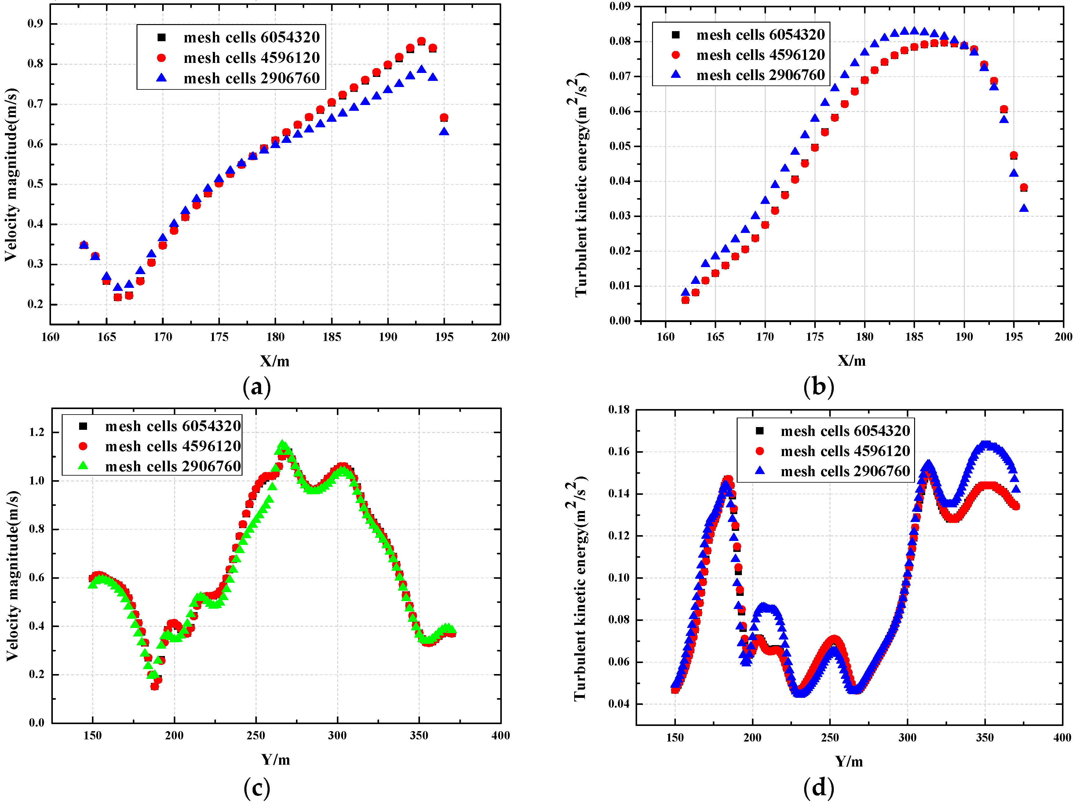
To capture the effects of grid independence to simulate the results, for this study, three types of grids (numbers 2906760, 4596120, and 6054320) were selected and calculated with the same computer under the same working conditions (wind speed v = 1.5 m/s, perpendicular to the street, and a source ratio of R = 2/1). We then selected a specific point in the computing domain, and found wind speeds of 1.571 m/s, 1.593 m/s, and 1.610 m/s under the three different grid numbers. The concentration levels of pollutants were 8.06 × 10⁻⁹, 7.84 × 10⁻⁹, and 7.67 × 10⁻⁹, respectively. In addition, the velocity magnitude and turbulent kinetic energy profile at a height of 2 m along the Y = 160 m section and the street centerline were compared in Figure 4. As can be seen from the figure, the maximum error appears at the turbulent kinetic energy profile at Y = 350 m, about 6%. Apart from this, Other errors are less than 5%. These results showed that further increasing the number of grids does not lead to apparent deviations of velocity and pollutant concentration, thus demonstrating precision of the numerical solution and irrelevance of the number of grids. The grid independence test results provide a good foundation for the remainder of the paper. Thus, mesh cells 4596120 were selected as the basic mesh system of this study.
2.6. Model Validation
To ensure accuracy and reliability of the numerical simulation, model validation is indispensable. Generally, to test the validity of a mathematical model that describes the fluid flow and the heat transfer characteristics of a specific system, the most feasible method is to compare numerical results to experimental results by providing both identical boundary and working conditions. However, many geometric models are too complex to find effective wind tunnel experimental data for comparison. The validation of the accuracy is aimed at testing the applicability of the RNG k-ε numerical model employed in this paper. Therefore, to validate the accuracy of the RNG k-ε numerical model we established another geometric model identical to the wind tunnel experiment model conducted by Takenobu et al. [49]. Experiments were conducted in a wind-tunnel facility (TWINNEL: twinned wind tunnel) at the Central Research Institute of Electric Power Industry (CRIEPI). The utilized wind tunnel is a closed-circuit. The experiment was conducted in the larger test section with dimensions of 17.0 m × 3.0 m × 1.7 m in streamwise (X), spanwise (Y), and vertical (Z) directions, respectively. Seven Irwin-type vortex generators with a height of 0.65 m were placed at the entrance of the test sections and three L-shaped cross-sections were located on the wind-tunnel floor from X = 0 to X = 5.0 m at equal intervals of 1.5 m to generate turbulent motions near the surface. A series of regularly spaced bars of 1.56 m (13 H) × 0.12 m (1 H) × 0.12 m (1 H) were set on the floor at equal intervals of H (0.12 m) from 10.5 m downwind of the entrance, normal to the wind direction. The origin of the coordinate axis forms the centre of the floor at the leeward wall of the 25th block, which is 16.62 m downwind of the entrance of the test section. The streamwise and vertical velocities at X/H = 0.25, 0.5, and 0.75 were measured in the vertical direction at Y/H = 0 using a laser Doppler velocimeter (LDV). The reference streamwise velocity at X/H = 0 and Z/H = 2.0 is 1.15 m/s. The pollutant emission rate Q is represented by a ground-level continuous pollutant line source of length Ly placed parallel to the spanwise axis at X/H = 0.5. The tracer gas ethane (it is both used in wind-tunnel experiment and current numerical simulation) is only emitted from a line source within the canyon. The upstream boundaries of the domain C|X=0 = 0 is applied and the stream at the outlet boundary emits the tracer gas out of the domain. That is, the free stream at the inlet boundary is free of pollutant. The concentration C is normalized by the freestream mean velocity U0 (1 m/s), block height H (0.12 m), line source length L (1.56 m), and total emission Q (10−7 kg/m3 s) as:
Using the same geometry and boundary conditions, we used the RNG k-ε numerical model for numerical calculation and compared the obtained results to experimental data. Vertical distributions of the streamwise velocity and normalized mean concentration at X/H = 0.50 are shown in Figure 5. Figure 5 shows that numerical simulation results of normalized mean concentration agree well with the experiment data. However, there is a small deviation in the vertical distribution of the streamwise velocity. The main reason may be due to the flow generated by the vortex generators in the wind tunnel experiment, which differs from the wind flow in the numerical simulation. Despite some slight differences, the RNG k-ε turbulence model is feasible for solving fluid flow and pollutant dispersion.
3. Results and Discussion
3.1. Impact Analysis of Non-Uniform Pollution Source
During both morning and evening, a two parallel road pollution source non-uniform distribution is caused by the impact of traffic tidal flow. This part focuses on the dispersion characteristics of pollutants under this specific case.
3.1.1. Concentration Distribution of CO at Pedestrian Breathing Height
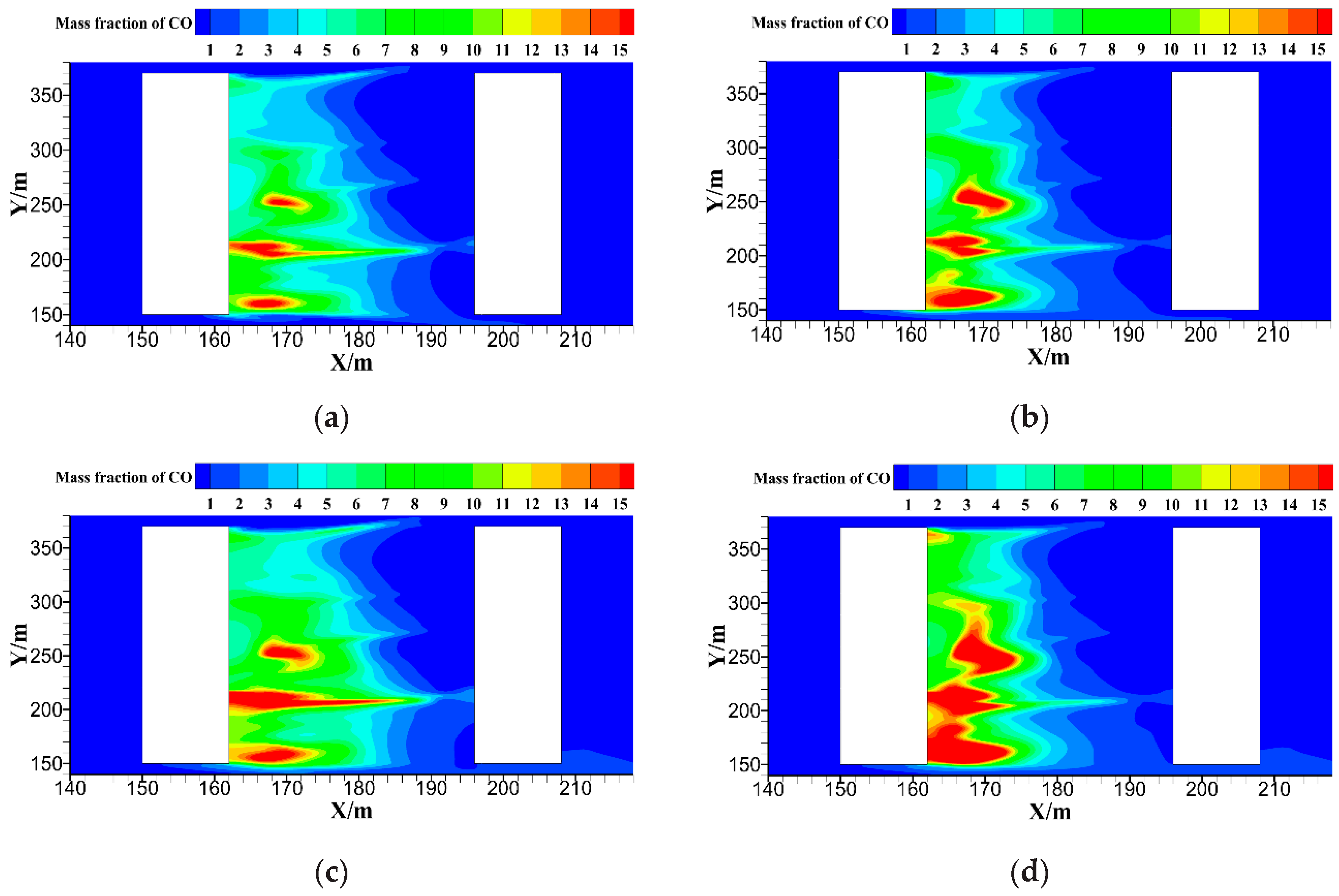
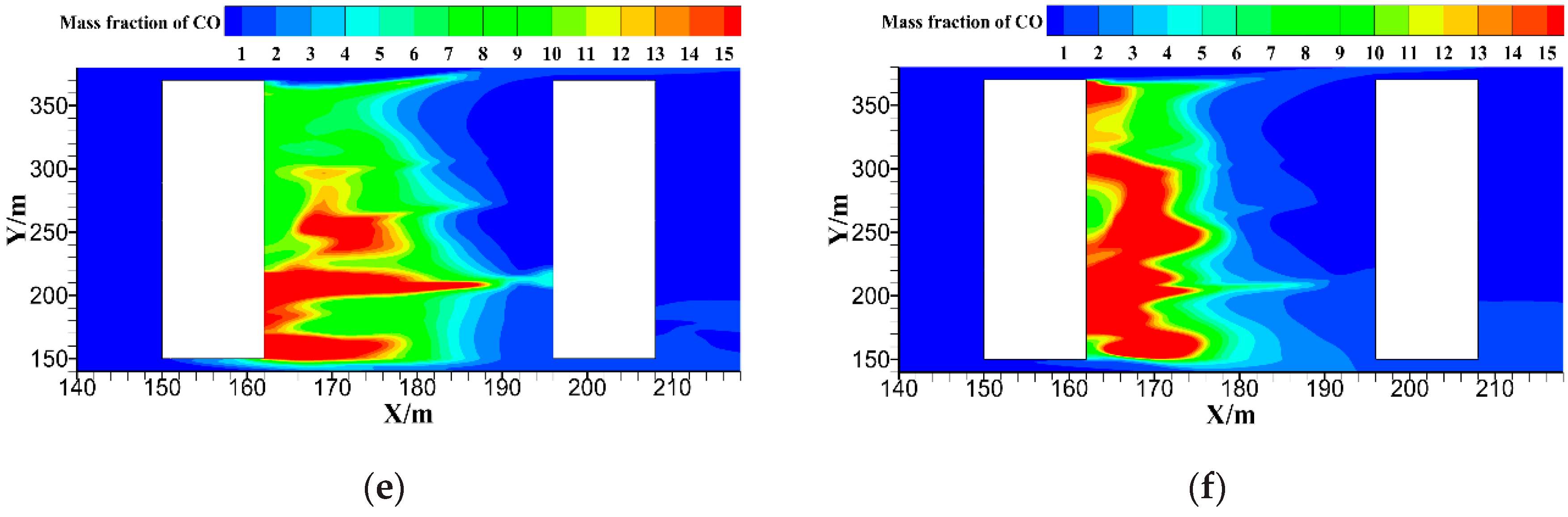
The wind speed 3 m/s, wind direction 90°, pollutant emission ratios 1/2, 1/3, 1/5, and the corresponding 2, 3, and 5 were chosen to show the distribution of CO concentration at the level Z = 1.5 m, which represents the pedestrian breathing height. Due to the asymmetrical arrangement of buildings in this street canyon, the flow field in the canyon becomes increasingly complicated. Figure 6 shows that CO mainly accumulates on the leeward side under the action of the perpendicular inlet wind. In some areas where the upstream building is higher than the downstream, a local high pollution level will appear. For the source distribution of R = 1/3 and R = 3, it can be found that even though the total source intensity in the street is equal, the stronger source at the left side in comparison to the right side (R = 3) will cause the expansion of the high pollution area. The results are found to be consistent when compared to the case of R = 1/2, R = 2 and R = 1/5, R = 5. Furthermore, this phenomenon becomes more apparent with increasing difference of source distribution between the two sides. Therefore, in the horizontal area of Z = 1.5 m in the street canyon, the increase of the pollution source near the leeward side will increase the range of the high pollution concentration area. Figure 7 shows the average concentration of CO at pedestrian breathing height under different pollution source distributions. A source intensity near the leeward side stronger than near the windward side (R = 2, R = 3, and R = 5) leads to an increase of the average concentration of CO by 26%, 37%, and 41%, respectively. The underlying causes of this phenomenon will be explained in Section 3.1.3.
3.1.2. Influence of Height Variation of Street Building on Non-Uniform Distribution Characteristics of the Pollution Source
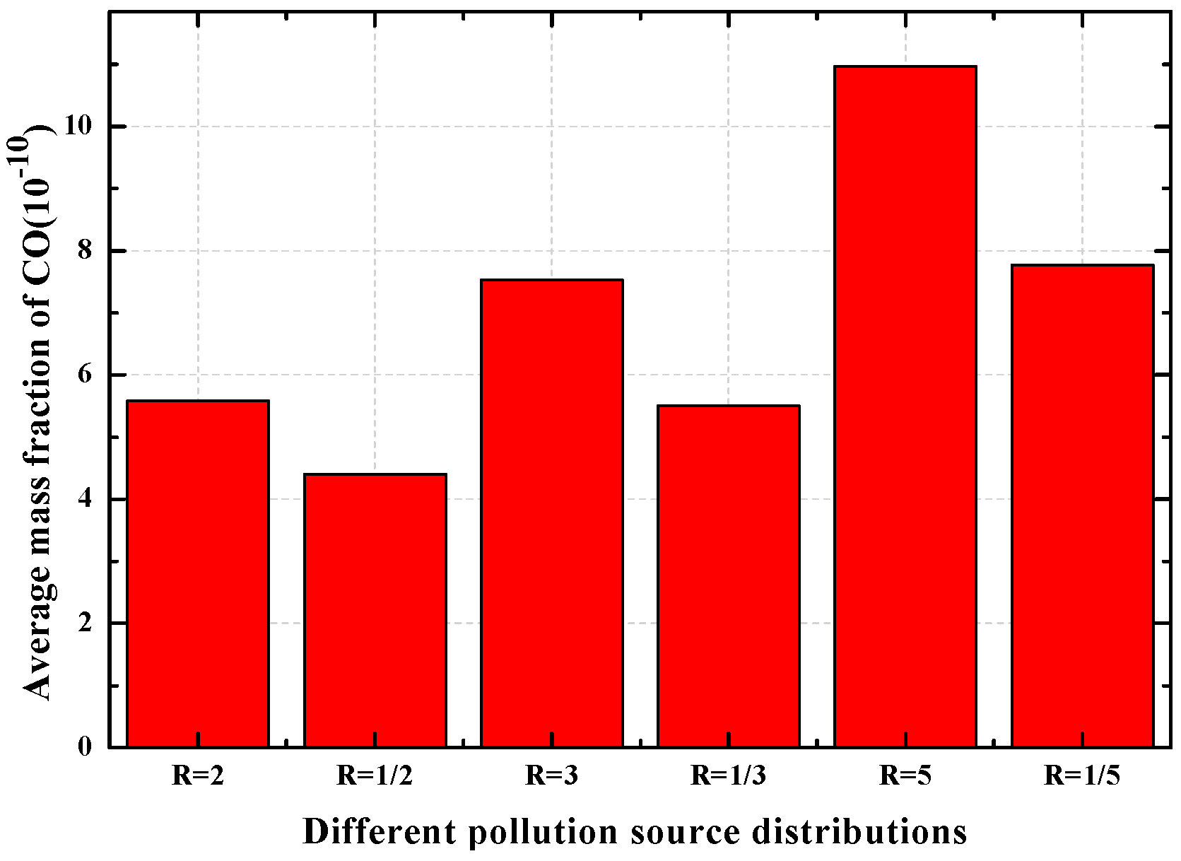
Through the above analysis of different source distributions in the street space at a horizontal height of 1.5 m, we found that high pollution areas appeared locally near the leeward surface. This was mainly related to the height of the buildings on both sides. To further analyze the influence of different building heights on the CO distribution characteristic, the section of Y = 160 m (the difference of building height on both sides is small), Y = 210 m (typical step-up canyon) and Y = 270 m (typical step-down canyon), pollution source intensity R = 1/3 and R = 3 were chosen. Under the lower wind speed condition, the pollutant dispersion was mainly affected by the geometric structure of the canyon; then, the wind speed was chosen to be 1.5 m/s.
In the Y = 160 m section, both sides are residential buildings, belonging to a densely populated area. From Figure 8a,b, it can be seen that the pollutant dispersion characteristics are very different even if the total source intensity would be equal in the street. The specific performance for the pollution source intensity for the left side (near the leeward side) was stronger than for the right side (near the windward side). The high pollution area presents approximately a quarter of a circle at the leeward side. However, when the source intensity at the right side was stronger than at the left side, the high pollution area presents a triangular trend from the leeward side to the center of the street. For a step-down canyon, the increase of source intensity at the right side expands the high pollution concentration area to the windward surface, which greatly increased the whole street space pollution. However, for the step-up canyon, due to the lower upstream building, the wind flow can soon eject pollutants out of the street. Therefore, in the step-up canyon, the impact of the pollution source non-uniform distribution on the pollutant dispersion characteristics is no longer significant.
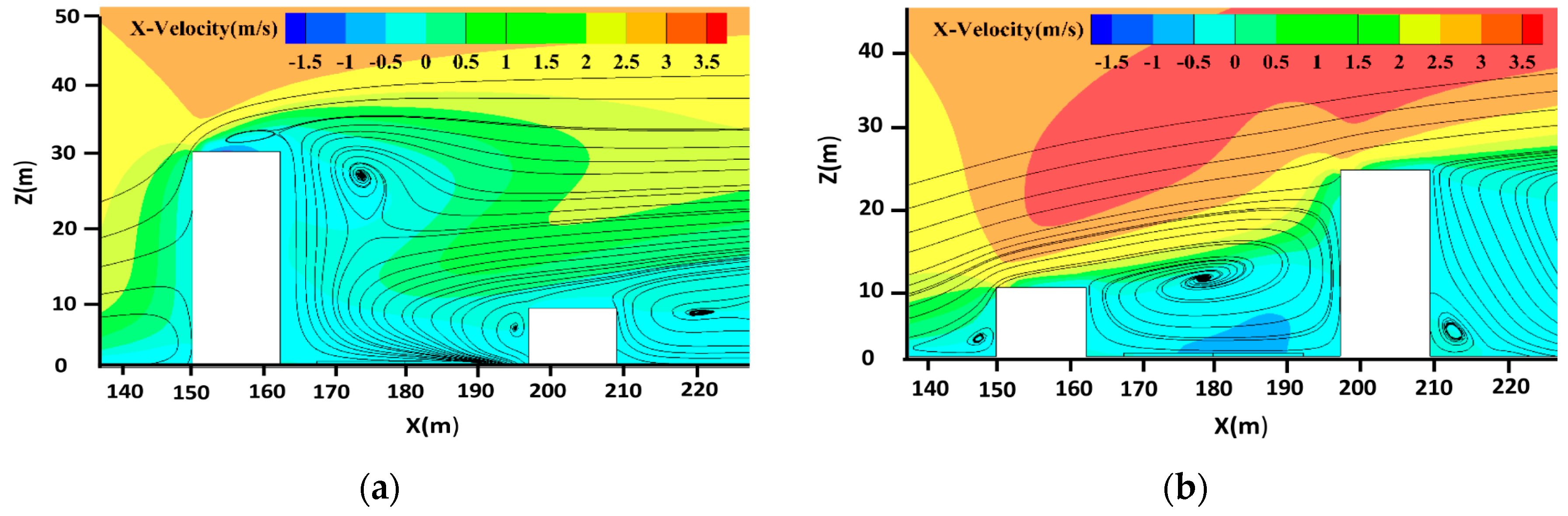
This phenomenon shown above is affected by flow field characteristics and the vortex intensity within the canyon. Figure 9a,b show the distribution of the streamlines in the street cross-section of Y = 210 m (typical step-up canyon) and Y = 270 m (typical step-down canyon) at a wind speed of 3 m/s. For the step-down canyon (Figure 9a), under the action of air transportation, CO accumulates in the leeward side of the street. Due to the increasing height of upstream buildings, the transportation ability of wind flow gradually decreases with increasing height in the leeward building surface. This leads to an accumulation of pollutants in the leeward side. For the step-up canyon (Figure 9b), a clockwise rotation vortex exists in the canyon due to the downstream building block air flow. The vortex center is located at half of the height of the downstream building. Under the action of vortex, the pollutants emitted by motor vehicles are transported from the windward side to the leeward side. Due to the relatively lower height of upstream buildings, CO can be quickly transported to the roof of the leeward surface, and will soon be diluted by the wind flow. The CO moving out of the canyon barely returns to the street. Thus, in the step-up canyon, the impact of the pollution source non-uniform distribution on the pollutant dispersion characteristics is no longer significant.
3.1.3. Analysis of Spatial Distribution Characteristics of CO Concentration in Specific Section
From the analysis in Section 3.1.1 and Section 3.1.2, it can be seen that both the pollution source distribution and the height variation of the buildings on both sides of the street influence the dispersion characteristics of the pollutant. To better understand the distribution of pollutants in the street space when the pollution source is non-uniform distribution, it is necessary to quantitatively analyze the pollutant concentration in the horizontal and vertical directions within the street canyon. However, due to the large computational domain, quantitative analysis is difficult to implement sequentially. Therefore, this paper selected the typical Y = 160 m cross-section in the street with the vertical direction X = 180 m (street center), X = 165 m, and X = 193 m (non-motorized road center in left and right side) and the horizontal direction Z = 1.5 m, Z = 5 m, and Z = 10 m as shown in Figure 10, to plot CO concentration curves at a wind speed of 1.5 m/s and wind direction 90°. Then, the distribution characteristics of CO in the horizontal and vertical street space were analyzed.
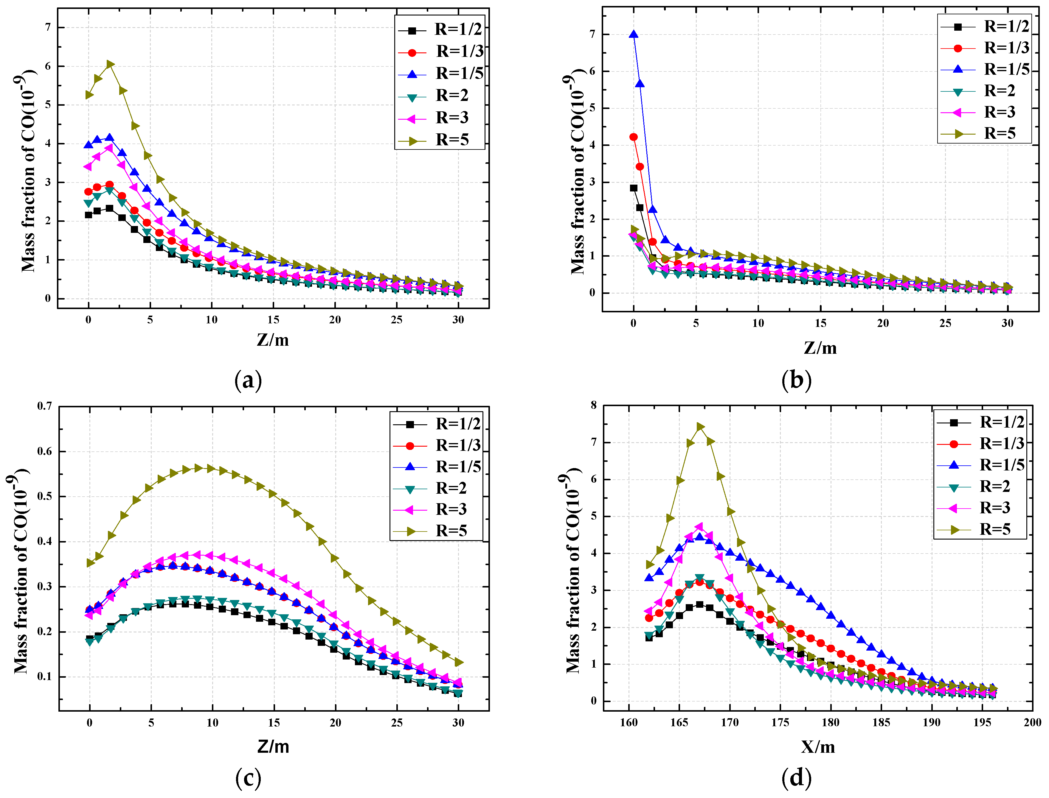
Firstly, the dispersion characteristics of CO in the vertical direction were analyzed when the pollution sources were non-uniformly distributed. Figure 11a shows the distribution of CO along the vertical direction of the non-motorized lane center near the leeward side. This analysis shows that, even though the total pollution source intensity in the street remained the same, the source intensity near the leeward side was stronger than near the windward side (R = 2, R = 3, and R = 5), increasing the CO concentration compared to the corresponding R = 1/2, R = 1/3, and R = 1/5 within the vertical direction of a 10 m height. Furthermore, a larger ratio leads to a more apparent difference in CO concentration. This was mainly because the source intensity near the leeward side had a decisive effect on the concentration of CO. Above a height of 10 m, the influence of non-uniform pollution source distribution basically disappeared. Both CO concentration curves of the same source intensity were basically consistent. With gradually increasing height, the impact of the total source intensity becomes inconspicuous. The CO level obtains a minimum value near the windward side. As the street center X = 180 m was close to the windward side, the CO concentration under the source distribution of R = 1/2, 1/3, and 1/5 was higher than the source distribution of R = 2, 3, and 5 within a height of 1 m. Since the wind force near the ground is relatively small, the CO concentration is mainly affected by the source intensity. However, soon the impact of both source intensity and non-uniform distribution have ceased. Since the vortex formed in the section, the pollutants are blown away from the windward side to the leeward side. Part of them spreads out of the canyon, while part of it accumulates at the leeward surface. Therefore, the CO concentration level in the vertical direction of the street center is neither affected by the source intensity nor by the non-uniform distribution. The concentration of CO is much smaller in the vicinity of the windward surface (X = 193 m), but the effect of pollution source non-uniform distribution is still present: When the source close to the leeward surface is strong, the CO concentration at the same height increases. The greater the ratio, the more obvious the difference in the concentration level will become (as shown in Figure 11c R = 1/5 and R = 5).
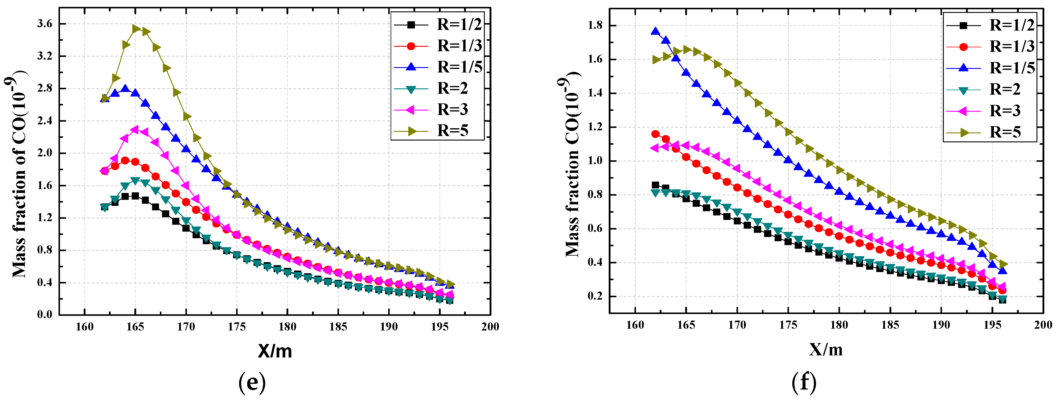
Figure 11d–f represent the CO concentration profiles at horizontal heights of Z = 1.5 m, Z = 5 m, and Z = 10 m, respectively. At the lower horizontal height (Z = 1.5 m), the concentration of CO is mainly dominated by the source intensity of both sides. In the vicinity of the leeward area (162 m < X < 172 m), the concentration of CO in the horizontal direction is high due to the stronger source intensity on the leeward side. With approaching the windward surface, the concentration of CO begin to change: the concentration of CO in the horizontal direction near the windward surface is high due to the stronger source intensity on the windward side. Finally, when the distance from the windward surface is very short, the impacts of pollution source intensity and non-uniform distribution cease. The concentration of CO in the windward surface reaches a minimum. In general, a stronger source intensity closer to the leeward than to the windward side will cause the expansion of the high pollution area. With increasing horizontal height (Z = 5 m), the CO concentration in the area near the leeward side is mainly dominated by the source intensity on the left side. However, as an approach to the windward surface, the impact of source non-uniform distribution basically disappeared. Furthermore, the two CO concentration distribution curves with the same total source intensities are beginning to be consistent. At the horizontal height of Z = 10 m (Figure 11f), a source intensity at left side stronger than at the right side (R = 2, 3, and 5) results in higher CO concentrations even though the total sources are equal.
The above analysis shows that when the pollution source is non-uniformly distributed, the concentration level of CO is mainly affected by the source intensity on both sides at a low horizontal height. As the height increases, the influence of source intensity gradually fades. Finally, a source intensity near the leeward side that is stronger than near the windward side will have a higher CO concentration level. This is mainly caused by the air vortex that formed in this section. The stream flows down along the windward building and begins to flow upward after passing the ground block. Pollutants near the windward area are more likely to be blown out of the street, while part of the pollutants near the leeward area enter the relatively small secondary-vortex which lies at the corner of the leeward surface. Pollutants in the small secondary-vortex are difficult to spread out of the canyon and result in a wide range of pollution areas within the street space. A further reason is due to the wind force near the windward side, which is usually stronger than the wind force near the leeward side. Then, pollutants near the windward side are more easily spread out of the canyon. Furthermore, when the source intensity near the leeward side is stronger, it will cause a large amount of pollutants to remain in the street canyon. Therefore, we can conclude that in the case of low wind speeds, a stronger source intensity near the leeward side easily forms a relatively large street pollution space.
3.2. Influence of Wind Speed and Wind Direction on the Non-Uniform Distribution of Pollution Sources
The above analyses about the dispersion characteristics of CO in the street canyon under non-uniform distribution of pollution source are based on a relatively low wind speed and for when the wind direction is perpendicular to the street. Therefore, it is necessary to analyze whether the influence of a non-uniformly distributed pollution source on the dispersion characteristics of pollutant remains significant under different wind speed and wind direction. We employed the pollution source emission ratios R = 1/5 and R = 5, wind speeds of V = 1.5 m/s, V = 3 m/s, V = 4.5 m/s, and V = 6 m/s, and a wind direction of 90° to analyze the impact of wind speed. Also, the pollution source emission ratios R = 1/5 and R = 5, wind speed V = 3 m/s, and wind direction 0°, 30°, 45°, and 60° were employed to analyze the impact of the wind direction. Then, the average concentration of CO at pedestrian breathing height Z = 1.5 m under different cases are shown in Figure 12.
According to Figure 12a, we firstly found that with increasing wind speeds, the average concentration of CO at the zone of pedestrian breathing height shows a decreasing trend. Furthermore, the characteristics of larger pollution space caused by stronger source intensity near the leeward side are also no longer significant with increasing wind speeds. I.e., the increasing wind speeds will weaken the effect of a non-uniform distribution of the pollution source on the dispersion characteristics of CO. The increasing wind speeds enhance the effect of wind force transportation and dilution, and accelerate the air exchange rate (ACH) between street canyon and the upper atmosphere. In addition, the wind force near the leeward side also enhanced with increasing wind speeds, and consequently, the pollutants near the leeward side are more likely to spread out of the canyon. This causes the phenomenon that larger pollution space caused by stronger source intensity near the leeward side is less significant with increasing wind speeds. Furthermore, when the wind direction is not perpendicular to the street, the effect of the non-uniform pollution source distribution on the dispersion characteristics of CO is also not significant. The average CO concentration remains the same under the two pollution source emission ratios of R = 1/5 and R = 5 as shown in Figure 12b. The wind direction determines the pollutant transport direction. For a wind direction of 0° or if it has a certain angle to the street axis, e.g., 30°, 45°, and 60°, then there is a velocity component on the Y-axis compared to the 90° wind direction. Then, the velocity component on the Y-axis will lead to a downward movement of pollutants along the street. Due to the absence of blocks downstream of the street, pollutants are easily dispersed. The parallel and oblique wind direction strengthens the spanwise (Y) direction dispersion of pollutants. Therefore, the effect of the non-uniform distribution of the pollution source on the dispersion characteristics of CO is no longer significant.
3.3. Influence of Source Intensity on Pollution Levels in Street Space
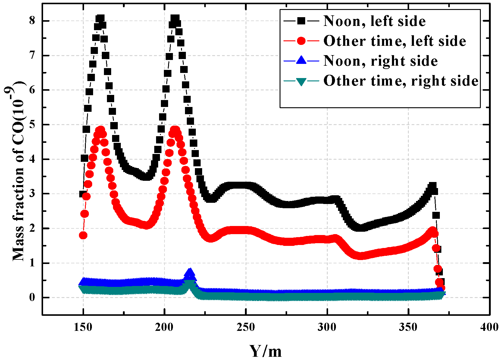
To analyze the influence of different pollution source intensities on the concentration of CO in the street, we employed the source intensity during noon (11:30–13:00) and other time (8:30–11:30 and 13:00–17:30) for the CFD numerical simulation. Then, the CO concentration levels along the center of two non-motorized lanes were plotted at a wind speed of 3 m/s. We mainly focused on the pedestrian breathing height of Z = 1.5 m. Through the field measurement we have obtained the source intensity during noon and at other times. These were 5.5 × 10⁻⁶ (kg/m3 s) and 3.3 × 10⁻⁷ (kg/m3 s).
Figure 13 shows a diagram of CO concentration levels along the center of two non-motorized lanes. The pollution source intensity significantly impacted the level of CO concentration. Through analysis of the CO concentration data, we found that with decreasing pollution source intensity, the average level of CO concentration at pedestrian breathing height decreased proportionally. At the left non-motorized center, the CO concentration decreased by about 30%. Furthermore, it decreased more at the right non-motorized center by about 40%. Thus, for the control of urban street vehicle pollution, the reduction of pollution source intensity is the most direct and effective way.
4. Conclusions
For this study, a three-dimensional geometrical model was established based on a street canyon section with a typical traffic tidal phenomenon in the 2nd Ring Road of Wuhan, China. A mathematical model describing the fluid flow and pollutant dispersion characteristics in the street canyon was developed. The number and driving speeds of vehicles on the road during different periods of one day were measured; then, the emission rate of pollutants in two parallel roads was calculated with the CFD simulation method. The results of the numerical simulation indicate that:
In this three-dimensional asymmetrical shallow street canyon, when pollution sources in the street are non-uniformly distributed and when the wind flow is perpendicular to the street, a stronger source intensity near the leeward side than near the windward side will cause the expansion of pollution space even though the total source intensity remains equal. For example, when the wind speed is 3 m/s, a source intensity near the leeward side stronger than near the windward side (R = 2, R = 3, and R = 5) increases the average concentration of CO at pedestrian breathing height increased by 26%, 37%, and 41%, respectively.
However, with increasing wind speeds and when the wind direction is not perpendicular to the street, the concentration of pollutants in the whole street space shows a decreasing trend. Furthermore, the characteristics of a larger pollution space caused by stronger source intensity near the leeward side were also less significant. I.e., the increase in wind speeds and changes in wind direction weakens the effect of pollution source non-uniform distribution on pollutant dispersion characteristics.
The source intensity significantly impacts the level of pollutant concentration in the street canyon. With decreasing source intensity, the level of pollutant concentration at pedestrian breathing level decreased proportionally. In the left non-motorized center, the CO concentration decreased by about 30%, while it decreased more at the right non-motorized center by about 40%. Thus, for the control of urban street vehicle pollution, a reduction of pollution source intensity is the most direct and effective way.
Acknowledgments
This research was supported by the National Natural Science Foundation of China (Nos. 51778511, 51778253), Key Project of ESI Discipline Development of Wuhan University of Technology (WUT No. 2017001), the Scientific Research Foundation of Wuhan University of Technology (No. 40120237).
Author Contributions
Tingzhen Ming and Chong Peng discussed and aroused the idea; Weijie Fang and Cunjin Cai performed the simulation; Weijie Fang drafted the manuscript; Tingzhen Ming, Renaud de Richter, Mohammad Hossein Ahmadi, and Yuangao Wen finalized the manuscript.
Conflicts of Interest
The authors declare no conflict of interest.
References
- Gong, T.; Ming, T.; Huang, X.; de Richter, R.K.; Wu, Y.; Liu, W. Numerical analysis on a solar chimney with an inverted U-type cooling tower to mitigate urban air pollution. Sol. Energy 2017, 147, 68–82. [Google Scholar] [CrossRef]
- Song, J.; Guang, W.; Li, L.; Xiang, R. Assessment of Air Quality Status in Wuhan, China. Atmosphere 2016, 7, 56. [Google Scholar] [CrossRef]
- Deng, Q.; Lu, C.; Yu, Y.; Li, Y.; Sundell, J.; Norbäck, D. Early life exposure to traffic-related air pollution and allergic rhinitis in preschool children. Respir. Med. 2016, 121, 67–73. [Google Scholar] [CrossRef] [PubMed]
- Deng, Q.; Chan, L.; Wei, J.; Zhao, J.; Deng, L.; Xiang, Y. Association of outdoor air pollution and indoor renovation with early childhood ear infection in China. Chemosphere 2017, 169, 288–296. [Google Scholar] [CrossRef] [PubMed]
- Nicholson, S.E. A pollution model for street-level air. Atmos. Environ. 1975, 9, 19. [Google Scholar] [CrossRef]
- Andreou, E.; Axarli, K. Investigation of urban canyon microclimate in traditional and contemporary environment. Experimental investigation and parametric analysis. Renew. Energy 2012, 43, 354–363. [Google Scholar] [CrossRef]
- Prajapati, S.K.; Tripathi, B.D.; Pathak, V. Distribution of vehicular pollutants in street canyons of Varanasi, India: A different case. Environ. Monit. Assess. 2009, 148, 167–172. [Google Scholar] [CrossRef] [PubMed]
- Salizzoni, P.; Soulhac, L.; Mejean, P. Street canyon ventilation and atmospheric turbulence. Atmos. Environ. 2009, 43, 5056–5067. [Google Scholar] [CrossRef]
- Allegrini, J.; Dorer, V.; Carmeliet, J. Wind tunnel measurements of buoyant flows in street canyons. Build. Environ. 2013, 59, 315–326. [Google Scholar] [CrossRef]
- Stabile, L.; Arpino, F.; Buonanno, G.; Russi, A.; Frattolillo, A. A simplified benchmark of ultrafine particle dispersion in idealized urban street canyons: A wind tunnel study. Build. Environ. 2015, 93, 186–198. [Google Scholar] [CrossRef]
- Wang, Y.; Huang, Z.; Liu, Y.; Yu, Q.; Ma, W. Back-Calculation of Traffic-Related PM10 Emission Factors Based on Roadside Concentration Measurements. Atmosphere 2017, 8, 99. [Google Scholar] [CrossRef]
- Chew, L.; Nazarian, N.; Norford, L. Pedestrian-Level Urban Wind Flow Enhancement with Wind Catchers. Atmosphere 2017, 8, 159. [Google Scholar] [CrossRef]
- Zhou, Y.; Deng, Q. Numerical simulation of inter-floor airflow and impact on pollutant transport in high-rise buildings due to buoyancy-driven natural ventilation. Indoor Built Environ. 2014, 23, 246–258. [Google Scholar] [CrossRef]
- Soulhac, L.; Mejean, P.; Perkins, R.J. Modelling the transport and dispersion of pollutants in street canyons. Int. J. Environ. Pollut. 2001, 16, 404–416. [Google Scholar] [CrossRef]
- Kim, J.J.; Baik, J.J. A numerical study of the effects of ambient wind direction on flow and dispersion in urban street canyons using the RNG—Turbulence model. Atmos. Environ. 2004, 38, 3039–3048. [Google Scholar] [CrossRef]
- Balogun, A.A.; Tomlin, A.S.; Wood, C.R.; Barlow, J.F.; Belcher, S.E.; Smalley, R.J.; Lingard, J.J.N.; Arnold, S.J.; Dobre, A.; Robins, A.G. In-Street Wind Direction Variability in the Vicinity of a Busy Intersection in Central London. Bound.-Layer Meteorol. 2010, 136, 489–513. [Google Scholar] [CrossRef]
- Kim, J.J.; Baik, J.J. Effects of inflow turbulence intensity on flow and pollutant dispersion in an urban street canyon. J. Wind Eng. Ind. Aerodyn. 2003, 91, 309–329. [Google Scholar] [CrossRef]
- Chan, A.T.; So, E.S.; Samad, S.C. Erratum to “Strategic guidelines for street canyon geometry to achieve sustainable street air quality” (Atmospheric Environment 35 (24) 4089–4098). Atmos. Environ. 2001, 35, 5679. [Google Scholar] [CrossRef]
- Chan, A.T.; So, E.S.; Samad, S.C. Strategic guidelines for street canyon geometry to achieve sustainable street air quality. Atmos. Environ. 2001, 35, 5681–5691. [Google Scholar] [CrossRef]
- Chang, C.H.; Meroney, R.N. Concentration and flow distributions in urban street canyons: Wind tunnel and computational data. J. Wind Eng. Ind. Aerodyn. 2003, 91, 1141–1154. [Google Scholar] [CrossRef]
- Liu, C.; Barth, M.C.; Leung, D.Y.C. Large-Eddy Simulation of Flow and Pollutant Transport in Street Canyons of Different Building-Height-to-Street-Width Ratios. J. Appl. Meteorol. 2004, 43, 1410–1424. [Google Scholar] [CrossRef]
- Kang, Y.S.; Baik, J.J.; Kim, J.J. Further studies of flow and reactive pollutant dispersion in a street canyon with bottom heating. Atmos. Environ. 2008, 42, 4964–4975. [Google Scholar] [CrossRef]
- Kim, J.J.; Baik, J.J. Effects of Street-Bottom and Building-Roof Heating on Flow in Three-Dimensional Street Canyons. Adv. Atmos. Sci. 2010, 27, 513–527. [Google Scholar] [CrossRef]
- Kim, J.J.; Pardyjak, E.; Kim, D.Y.; Han, K.S.; Kwon, B.H. Effects of building-roof cooling on flow and air temperature in urban street canyons. Asia Pac. J. Atmos. Sci. 2014, 50, 365–375. [Google Scholar] [CrossRef]
- Gronemeier, T.; Raasch, S.; Ng, E. Effects of Unstable Stratification on Ventilation in Hong Kong. Atmosphere 2017, 8, 168. [Google Scholar] [CrossRef]
- Lateb, M.; Meroney, R.N.; Yataghene, M.; Fellouah, H.; Saleh, F.; Boufadel, M.C. On the use of numerical modelling for near-field pollutant dispersion in urban environments—A review. Environ. Pollut. 2016, 208, 271–283. [Google Scholar] [CrossRef] [PubMed]
- Nosek, Š.; Kukačka, L.; Kellnerová, R.; Jurčáková, K.; Jaňour, Z. Ventilation Processes in a Three-Dimensional Street Canyon. Bound.-Layer Meteorol. 2016, 159, 1–26. [Google Scholar] [CrossRef]
- Gu, Z.; Zhang, Y.; Cheng, Y.; Lee, S.C. Effect of uneven building layout on air flow and pollutant dispersion in non-uniform street canyons. Build. Environ. 2011, 46, 2657–2665. [Google Scholar] [CrossRef]
- Nosek, Š.; Kukačka, L.; Jurčáková, K.; Kellnerová, R.; Jaňour, Z. Impact of roof height non-uniformity on pollutant transport between a street canyon and intersections. Environ. Pollut. 2017, 227, 125. [Google Scholar] [CrossRef] [PubMed]
- Tominaga, Y.; Mochida, A.; Yoshie, R.; Kataoka, H.; Nozu, T.; Yoshikawa, M.; Shirasawa, T. AIJ guidelines for practical applications of CFD to pedestrian wind environment around buildings. J. Wind Eng. Ind. Aerodyn. 2008, 96, 1749–1761. [Google Scholar] [CrossRef]
- Ming, T.; Gong, T.; Peng, C.; Li, Z. Pollutant Dispersion in Built Environment; Springer: Singapore, 2017. [Google Scholar]
- de_Richter, R.; Ming, T.; Davies, P.; Liu, W.; Caillol, S. Removal of non-CO2 greenhouse gases by large-scale atmospheric solar photocatalysis. Prog. Energy Combust. Sci. 2017, 60, 68–96. [Google Scholar] [CrossRef]
- Chan, T.L.; Dong, G.; Leung, C.W.; Cheung, C.S.; Hung, W.T. Validation of a two-dimensional pollutant dispersion model in an isolated street canyon. Atmos. Environ. 2002, 36, 861–872. [Google Scholar] [CrossRef]
- Blocken, B.; Stathopoulos, T.; Saathoff, P.; Wang, X. Numerical evaluation of pollutant dispersion in the built environment: Comparisons between models and experiments. J. Wind Eng. Ind. Aerodyn. 2008, 96, 1817–1831. [Google Scholar] [CrossRef] [Green Version]
- Nazridoust, K.; Ahmadi, G. Airflow and pollutant transport in street canyons. J. Wind Eng. Ind. Aerodyn. 2006, 94, 491–522. [Google Scholar] [CrossRef]
- Blocken, B.; Stathopoulos, T.; Carmeliet, J.; Hensen, J.L.M. Application of computational fluid dynamics in building performance simulation for the outdoor environment: An overview. J. Build. Perform. Simul. 2011, 4, 157–184. [Google Scholar] [CrossRef]
- Tominaga, Y.; Stathopoulos, T. CFD modeling of pollution dispersion in a street canyon: Comparison between LES and RANS. J. Wind Eng. Ind. Aerodyn. 2011, 99, 340–348. [Google Scholar] [CrossRef]
- Xie, X.; Liu, C.H.; Leung, D.Y.C.; Leung, M.K.H. Characteristics of air exchange in a street canyon with ground heating. Atmos. Environ. 2006, 40, 6396–6409. [Google Scholar] [CrossRef]
- Xie, X.; Liu, C.H.; Leung, D.Y.C. Impact of building facades and ground heating on wind flow and pollutant transport in street canyons. Atmos. Environ. 2007, 41, 9030–9049. [Google Scholar] [CrossRef]
- Hang, J.; Li, S. Effect Of Urban Morphology On Wind Condition In Idealized City Models. Atmos. Environ. 2009, 43, 869–878. [Google Scholar] [CrossRef]
- Yakhot, V.; Orszag, S.A. Renormalization group and local order in strong turbulence. Nucl. Phys. B 1987, 2, 417–440. [Google Scholar] [CrossRef]
- Li, X.; Liu, C.H.; Leung, D.Y.C. Development of a k–ε model for the determination of air exchange rates for street canyons. Atmos. Environ. 2005, 39, 7285–7296. [Google Scholar] [CrossRef]
- Hang, J.; Li, Y.; Sandberg, M.; Buccolieri, R.; Sabatino, S.D. The influence of building height variability on pollutant dispersion and pedestrian ventilation in idealized high-rise urban areas. Build. Environ. 2012, 56, 346–360. [Google Scholar] [CrossRef]
- Rajapaksha, I.; Nagai, H.; Okumiya, M. A ventilated courtyard as a passive cooling strategy in the warm humid tropics. Renew. Energy 2003, 28, 1755–1778. [Google Scholar] [CrossRef]
- Leung, K.K.; Liu, C.H.; Wong, C.C.C.; Lo, J.C.Y.; Ng, G.C.T. On the study of ventilation and pollutant removal over idealized two-dimensional urban street canyons. Build. Simul. 2012, 5, 359–369. [Google Scholar] [CrossRef]
- Wang, H.; Chen, Q. A new empirical model for predicting single-sided, wind-driven natural ventilation in buildings. Energy Build. 2012, 54, 386–394. [Google Scholar] [CrossRef]
- Zhang, K.; Yao, L. Research on the relationship between driving behavior and exhaust emission. Highw. Automot. Appl. 2014, 160, 39–43. [Google Scholar]
- Patankar, S.V. Numerical Heat Transfer and Fluid Flow; CRC press: Boca Raton, FL, USA, 1980; pp. 125–126. [Google Scholar]
- Michioka, T.; Takimoto, H.; Kanda, M. Large-Eddy Simulation for the Mechanism of Pollutant Removal from a Two-Dimensional Street Canyon. Bound.-Layer Meteorol. 2011, 138, 195–213. [Google Scholar] [CrossRef]
Figure 1.
Tidal phenomenon of urban road traffic (Photo was taken on Wednesday, 9 November 2016 at 7:23 a.m.).
Figure 1.
Tidal phenomenon of urban road traffic (Photo was taken on Wednesday, 9 November 2016 at 7:23 a.m.).
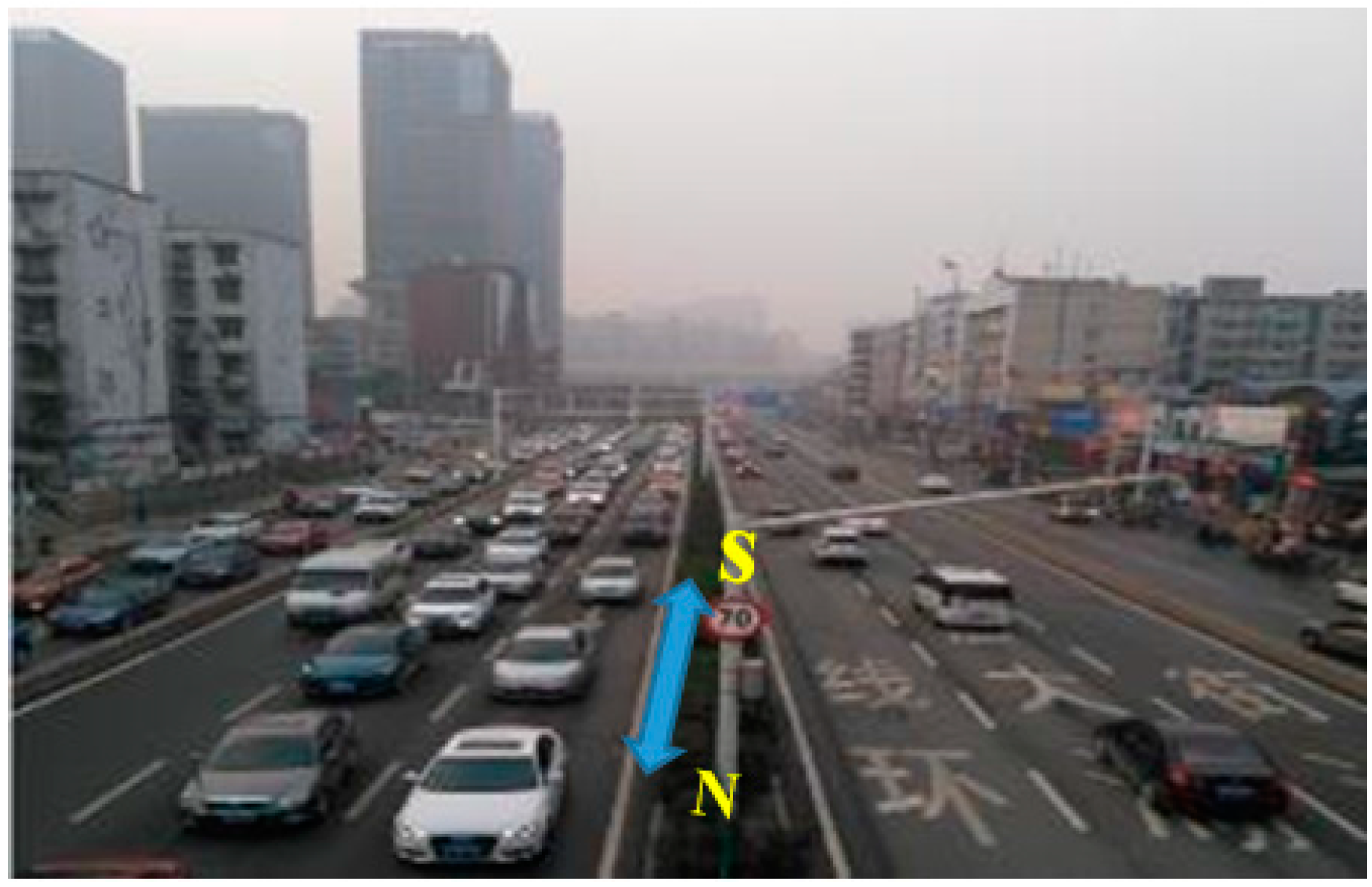
Figure 2.
Street canyon model (a) computing domain model and the boundary conditions; (b) building geometric structure.
Figure 2.
Street canyon model (a) computing domain model and the boundary conditions; (b) building geometric structure.

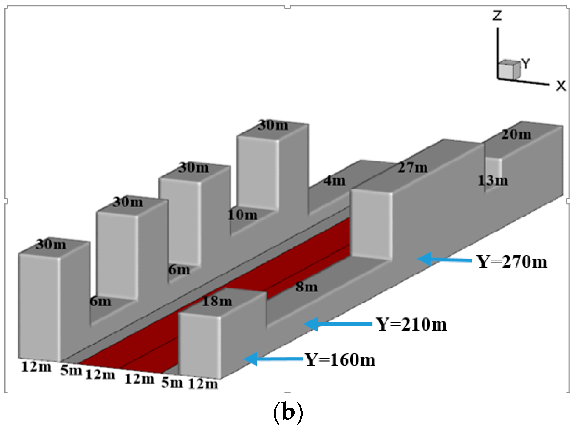
Figure 3.
Schematic diagram of grid demarcation in a cross-section.
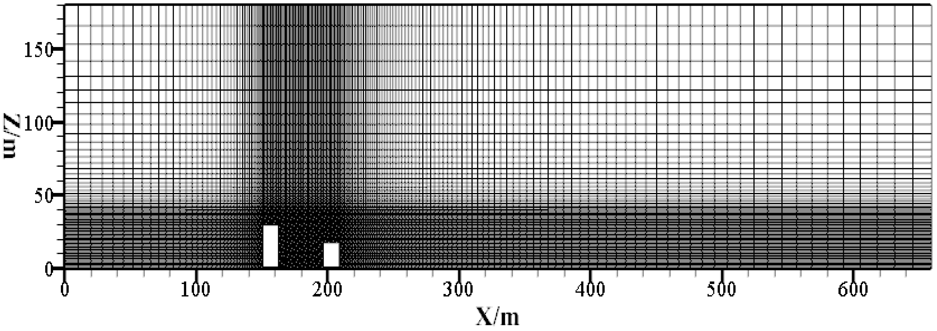
Figure 4.
Velocity magnitude and turbulent kinetic energy profile at a height of 2 m along the Y = 160 m section and the street centerline. (a) velocity magnitude profile along the Y = 160 m section; (b) turbulent kinetic energy profile along the Y = 160 m section; (c) velocity magnitude profile along the street centerline; (d) turbulent kinetic energy profile along the street centerline.

Figure 5.
Vertical distributions of streamwise velocity (a) and normalized mean concentration (b) at x/H = 0.50.
Figure 5.
Vertical distributions of streamwise velocity (a) and normalized mean concentration (b) at x/H = 0.50.
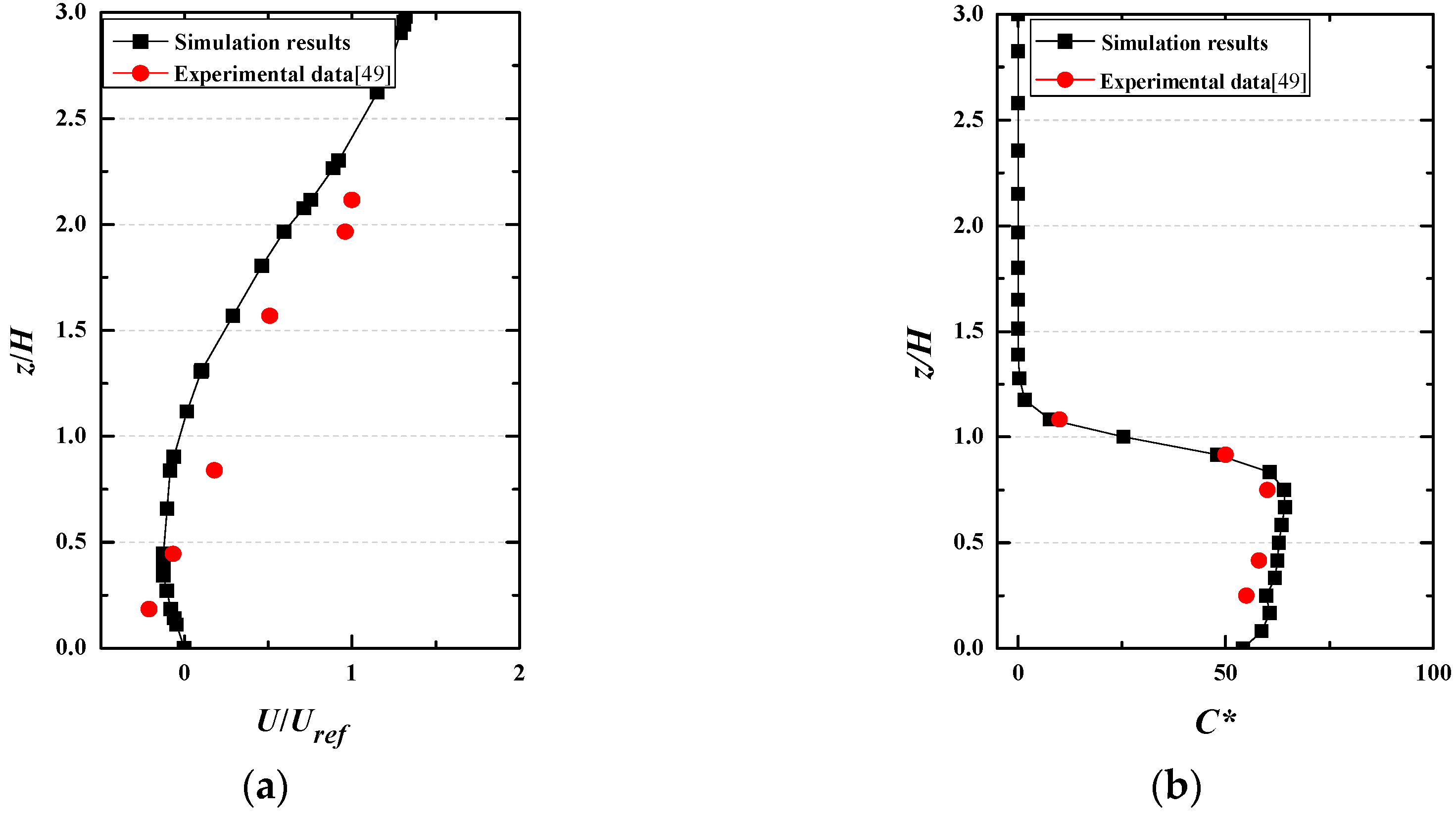
Figure 6.
CO concentration field profiles (10−9) in the street space for different pollution source distributions under a wind speed of 3 m/s. (a) R = 1/2; (b) R = 2; (c) R = 1/3; (d) R = 3; (e) R = 1/5; (f) R = 5.
Figure 6.
CO concentration field profiles (10−9) in the street space for different pollution source distributions under a wind speed of 3 m/s. (a) R = 1/2; (b) R = 2; (c) R = 1/3; (d) R = 3; (e) R = 1/5; (f) R = 5.


Figure 7.
The average concentration of CO at pedestrian breathing height under different pollution source distributions.
Figure 7.
The average concentration of CO at pedestrian breathing height under different pollution source distributions.

Figure 8.
CO concentration field profile (10−9) in three different sections at a wind speed of 1.5 m/s and emission ratios of R = 1/3 and R = 3. (a) Y = 160 m, R = 1/3; (b) Y = 160 m, R = 3; (c) Y = 210 m, R = 1/3; (d) Y = 210 m, R = 3; (e) Y = 270 m, R = 1/3; (f) Y = 270 m, R = 3.
Figure 8.
CO concentration field profile (10−9) in three different sections at a wind speed of 1.5 m/s and emission ratios of R = 1/3 and R = 3. (a) Y = 160 m, R = 1/3; (b) Y = 160 m, R = 3; (c) Y = 210 m, R = 1/3; (d) Y = 210 m, R = 3; (e) Y = 270 m, R = 1/3; (f) Y = 270 m, R = 3.

Figure 9.
Schematic diagram of the streamline at a wind speed of 3 m/s: (a) Y = 210 m section; (b) Y = 270 m section.
Figure 9.
Schematic diagram of the streamline at a wind speed of 3 m/s: (a) Y = 210 m section; (b) Y = 270 m section.

Figure 10.
Selected line diagram of vertical and horizontal directions in the Y = 160 m section. (a) Vertical direction; (b) Horizontal direction.
Figure 10.
Selected line diagram of vertical and horizontal directions in the Y = 160 m section. (a) Vertical direction; (b) Horizontal direction.

Figure 11.
CO concentration profile at different spatial positions at the wind speed 1.5 m/s: (a) X = 165 m; (b) X = 180 m; (c) X = 193 m; (d) Z = 1.5 m; (e) Z = 5 m; (f) Z = 10 m.
Figure 11.
CO concentration profile at different spatial positions at the wind speed 1.5 m/s: (a) X = 165 m; (b) X = 180 m; (c) X = 193 m; (d) Z = 1.5 m; (e) Z = 5 m; (f) Z = 10 m.


Figure 12.
Average concentration of CO at pedestrian breathing height under different wind speeds (a) and wind direction (b).
Figure 12.
Average concentration of CO at pedestrian breathing height under different wind speeds (a) and wind direction (b).
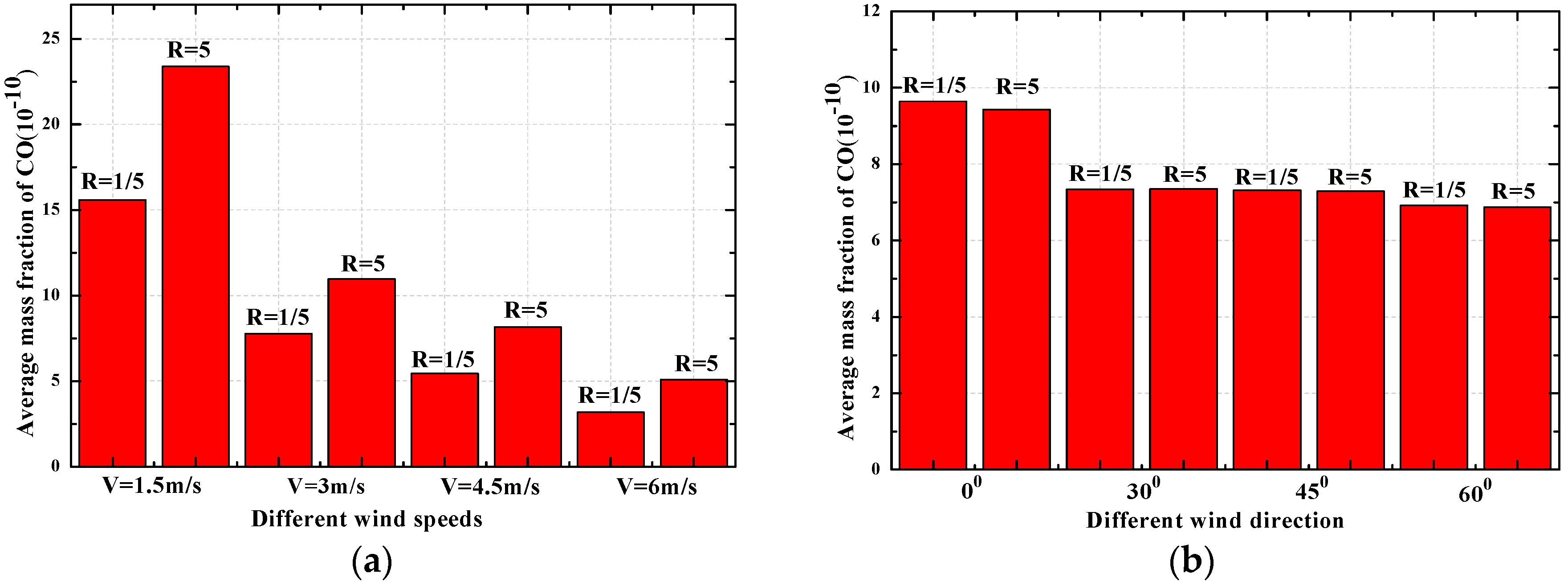
Figure 13.
CO concentration profile at a height of Z = 1.5 m at the left and right sides of the non-motorized center.
Figure 13.
CO concentration profile at a height of Z = 1.5 m at the left and right sides of the non-motorized center.

Table 1.
Relationship between driving speed and emission rate [47].
Table 1.
Relationship between driving speed and emission rate [47].
| Speed Range km/h | Emission Rate mg/(veh s) | ||
|---|---|---|---|
| NOx | HC | CO | |
| 0–10 | 0.20013 | 0.53241 | 5.90124 |
| 10–20 | 0.67005 | 1.01235 | 19.86452 |
| 20–30 | 1.65470 | 1.05106 | 22.14546 |
| 30–40 | 2.03404 | 1.10454 | 23.14653 |
| 40–50 | 3.10247 | 1.22414 | 26.15460 |
| 50–60 | 2.75461 | 1.45127 | 24.15641 |
| 60–70 | 4.05120 | 1.10021 | 14.48432 |
| 70–80 | 4.16471 | 1.01145 | 9.08424 |
| 80–90 | 3.45153 | 1.02104 | 4.11461 |
| 90–100 | 2.13451 | 1.01412 | 2.21457 |
| >100 | 1.02465 | 1.01214 | 0.94564 |
Table 2.
Experimental values of pollution source intensity at different times during one day.
| Experimental Value | Time | Morning | Evening | Noon | Other Times |
| 6:00–8:30 | 17:30–20:00 | 11:30–13:00 | 8:30–11:30 | ||
| 13:00–17:30 | |||||
| Traffic flow on the left side (vehicle) | 62 | 30 | 30 | 16 | |
| Driving speed on the left side (km/h) | 11 | 25 | 25 | 40 | |
| CO emission rate (mg/s) | 19.86 | 22.14 | 22.15 | 26.15 | |
| Pollution source intensity on the left side (kg/m3 s) | 9.93 × 10⁻⁷ | 5.5 × 10⁻⁷ | 5.5 × 10⁻⁷ | 3.3 × 10⁻⁷ | |
| Traffic flow on the right side (vehicle) | 28 | 72 | 30 | 16 | |
| Driving speed on the right side (km/h) | 25 | 11 | 25 | 40 | |
| CO emission rate (mg/s) | 22.14 | 19.86 | 22.15 | 26.15 | |
| Pollution source intensity on the right side (kg/m3 s) | 5.54 × 10⁻⁷ | 1.15 × 10⁻⁶ | 5.5 × 10⁻⁷ | 3.3 × 10⁻⁷ |
Table 3.
Simulation setting value of pollution source on both sides.
| Pollution Source at the Left Side (kg/m3 s) | Pollution Source at the Right Side (kg/m3 s) |
|---|---|
| 2 × 10⁻⁷ | 1 × 10⁻⁷ |
| 3 × 10⁻⁷ | 1 × 10⁻⁷ |
| 5 × 10⁻⁷ | 1 × 10⁻⁷ |
| 1 × 10⁻⁷ | 2 × 10⁻⁷ |
| 1 × 10⁻⁷ | 3 × 10⁻⁷ |
| 1 × 10⁻⁷ | 5 × 10⁻⁷ |
© 2018 by the authors. Licensee MDPI, Basel, Switzerland. This article is an open access article distributed under the terms and conditions of the Creative Commons Attribution (CC BY) license (http://creativecommons.org/licenses/by/4.0/).
Share and Cite
MDPI and ACS Style
Ming, T.; Fang, W.; Peng, C.; Cai, C.; De Richter, R.; Ahmadi, M.H.; Wen, Y. Impacts of Traffic Tidal Flow on Pollutant Dispersion in a Non-Uniform Urban Street Canyon. Atmosphere 2018, 9, 82. https://doi.org/10.3390/atmos9030082
AMA Style
Ming T, Fang W, Peng C, Cai C, De Richter R, Ahmadi MH, Wen Y. Impacts of Traffic Tidal Flow on Pollutant Dispersion in a Non-Uniform Urban Street Canyon. Atmosphere. 2018; 9(3):82. https://doi.org/10.3390/atmos9030082
Chicago/Turabian StyleMing, Tingzhen, Weijie Fang, Chong Peng, Cunjin Cai, Renaud De Richter, Mohammad Hossein Ahmadi, and Yuangao Wen. 2018. "Impacts of Traffic Tidal Flow on Pollutant Dispersion in a Non-Uniform Urban Street Canyon" Atmosphere 9, no. 3: 82. https://doi.org/10.3390/atmos9030082
Note that from the first issue of 2016, this journal uses article numbers instead of page numbers. See further details here.