Comprehensive Evaluation of Machine Learning Techniques for Estimating the Responses of Carbon Fluxes to Climatic Forces in Different Terrestrial Ecosystems


1
Key Laboratory of Coalbed Methane Resources and Reservoir Formation Process of the Ministry of Education, China University of Mining and Technology, Xuzhou 221116, China
2
School of Resources and Geosciences, China University of Mining and Technology, Xuzhou 221116, China
*
Author to whom correspondence should be addressed.
Atmosphere 2018, 9(3), 83; https://doi.org/10.3390/atmos9030083
Submission received: 15 December 2017
/
Revised: 11 February 2018
/
Accepted: 22 February 2018
/
Published: 25 February 2018
(This article belongs to the Special Issue Weather and Climate Change Challenges in Agricultural and Forest Meteorology)
Abstract
:Accurately estimating the carbon budgets in terrestrial ecosystems ranging from flux towers to regional or global scales is particularly crucial for diagnosing past and future climate change. This research investigated the feasibility of two comparatively advanced machine learning approaches, namely adaptive neuro-fuzzy inference system (ANFIS) and extreme learning machine (ELM), for reproducing terrestrial carbon fluxes in five different types of ecosystems. Traditional artificial neural network (ANN) and support vector machine (SVM) models were also utilized as reliable benchmarks to measure the generalization ability of these models according to the following statistical metrics: coefficient of determination (R2), index of agreement (IA), root mean square error (RMSE), and mean absolute error (MAE). In addition, we attempted to explore the responses of all methods to their corresponding intrinsic parameters in terms of the generalization performance. It was found that both the newly proposed ELM and ANFIS models achieved highly satisfactory estimates and were comparable to the ANN and SVM models. The modeling ability of each approach depended upon their respective internal parameters. For example, the SVM model with the radial basis kernel function produced the most accurate estimates and performed substantially better than the SVM models with the polynomial and sigmoid functions. Furthermore, a remarkable difference was found in the estimated accuracy among different carbon fluxes. Specifically, in the forest ecosystem (CA-Obs site), the optimal ANN model obtained slightly higher performance for gross primary productivity, with R2 = 0.9622, IA = 0.9836, RMSE = 0.6548 g C m−2 day−1, and MAE = 0.4220 g C m−2 day−1, compared with, respectively, 0.9554, 0.9845, 0.4280 g C m−2 day−1, and 0.2944 g C m−2 day−1 for ecosystem respiration and 0.8292, 0.9306, 0.6165 g C m−2 day−1, and 0.4407 g C m−2 day−1 for net ecosystem exchange. According to the findings in this study, we concluded that the proposed ELM and ANFIS models can be effectively employed for estimating terrestrial carbon fluxes.
1. Introduction
Terrestrial ecosystems play a vital role in sequestering the carbon dioxide in the atmosphere [1,2]. In general, the amount of carbon sequestration in different terrestrial ecosystems varies on seasonal, annual, and inter-annual time scales [3]. To account for this, the responses of terrestrial carbon exchanges to global environmental change involving climate extremes such as windstorms, heat waves, frosts and droughts, and a variety of disturbances, mainly including land use changes, fires, nitrogen deposition, and CO2 elevation, have recently attracted much attention [4,5,6]. These drivers may alter the composition, structure, and function of terrestrial ecosystems [7] and subsequently influence the magnitude and behavior of carbon cycles and their feedbacks to global change [8,9]. The inability of sufficiently characterizing the ongoing evolution of carbon fluxes using different techniques has been a primary impediment in our understanding of the underlying mechanisms in terrestrial carbon exchange processes [10,11,12]. For this reason, it is crucial to accurately estimate the carbon budgets in terrestrial ecosystems ranging from flux towers to regional or global scales for diagnosing past and future climate change.
To date, most prior studies that examine the roles of the aforementioned drivers and assess their induced uncertainties in the terrestrial carbon flux estimation have relied primarily upon the process-based models through describing complex biological and physical processes [13,14]. In general, the precision and reliability of these models are severely hindered due to the underlying nonlinear and nonstationary characteristics of terrestrial ecosystems. In contrast to process-based models, Schindler and Hilborn [15] suggested that mechanism-free models constitute the best alternative technology; such models depend upon constantly changing statistical characteristics of pooled data for short-term projections. Ye et al. [16] demonstrated the superiority of empirical dynamic modeling over static equilibrium-based models with deterministic rules and parameters, due to the fact that the former is viewed as an equation-free mechanistic forecasting technology, with the capability of adjusting both non-equilibrium dynamics and nonlinearities in natural ecosystems. The potential and versatility of machine learning techniques has been widely acknowledged with respect to solving the complex nonlinear problems [17,18] in the field of eco-informatics in the context of data-intensive ecological sciences [19]. Motivated by this and the recent availability of large amounts of accumulated data measured by the eddy covariance technique from flux tower networks across different vegetation types, the present research was undertaken to imitate the nonlinear relationships between carbon fluxes and environmental variables using machine learning approaches.
Over the past decades, machine learning techniques have gained great attention for dealing with different nonlinear issues in the ecological, climatological, and environmental fields, such as above-ground biomass estimation [20], methane emission prediction [21], meteorological anomaly detection [22], and biophysical parameter retrieval from remote sensing data [23]. In fact, the carbon exchanges of terrestrial ecosystems are complex nonlinear processes, which are predominantly controlled by environmental variables (e.g., solar radiation, air temperature, wind speed, and relative humidity). For this reason, the use of machine learning techniques was taken into consideration to characterize the carbon exchange processes between land and the atmosphere. In recent years, several lines of evidence have illustrated that machine learning techniques are able to perform better than some physically based models in terms of estimating the terrestrial carbon fluxes at different spatial and temporal scales [14,24,25]. Among machine learning techniques, two prominent approaches are the artificial neural network (ANN) and the support vector machine (SVM). They have been broadly utilized by previous studies for estimating terrestrial carbon fluxes [26,27,28].
Despite the increased use of machine learning techniques for simulating carbon fluxes, it is particularly important to note that the operability, robustness, and predictability of these techniques, especially for the ubiquitous ANN and SVM, may be limited by their respective disadvantages. Specifically, the ANN method still suffers from several drawbacks [29], such as over-fitting, local minima, and many inner parameters that need to be determined (e.g., the number of nodes in the hidden layer and the selection of training function), while the major drawbacks of SVM include a long computing time during the training process as well as a high memory requirement for solving problems of large-scale quadratic programming [30]. To address the shortcomings of these supervised learning-based approaches, a number of novel methods have been proposed in recent years. Among these methods, two advanced modeling techniques, namely the extreme learning machine (ELM) and the adaptive neuro-fuzzy inference system (ANFIS), are considered here due to their innovative design features, extremely fast convergence rate, and high performance. Some recent applications of these two relatively new methods in a wide variety of fields include solar radiation prediction [31,32], wind power prediction [33,34,35], stream-flow forecasting [36,37], and reference evapotranspiration prediction [38,39]. To the best of our knowledge, no research has yet been conducted that applies both the ELM and AFNIS methods to predict terrestrial carbon fluxes.
Many existing practical applications of the aforementioned methods in other different fields have suggested that the modeling and predictive capability of these approaches strongly depends on their respective internal parameters, despite the fact that they may provide some satisfactory results for a given problem. It seems quite evident that comparing and evaluating the ability of different parameters or functions for each approach is an outstanding prerequisite for removing their influences. For example, Tezel and Buyukyildiz [40] evaluated the effects of four different training algorithms used in the ANN method for predicting monthly pan evaporation that make use of several climatic variables—(1) resilient backpropagation, (2) scaled conjugate gradient (SCG), (3) Levenberg–Marquardt and gradient descent with momentum, and (4) adaptive learning rule backpropagation—and found that obvious differences existed among these training algorithms and that the SCG algorithm provided the best estimates. Moosavi et al. [41] compared the ability of an ANN with six different training algorithms and the ANFIS with four different membership functions to forecast monthly groundwater level and reported that the Bayesian regularization algorithm and the bell-shaped function generated the best results for the ANN and ANFIS methods, respectively. In a word, there is still great interest in identifying optimal inner algorithm for ensuring a method’s accuracy and stability for a given application. In particular, the predictive ability of these methods responding to their respective intrinsic parameters has not yet been appraised.
Taking the above-mentioned considerations into account, the objectives of the present research are fourfold: (1) to explore the adaptability and potential of the ELM and ANFIS methods in estimating daily carbon fluxes across five different types of terrestrial ecosystems; (2) to compare the predictive accuracy of our newly developed approaches with conventional ANN and SVM methods; (3) to evaluate the effects of internal parameters of each method on their respective generalization ability; and (4) to probe into the modeling difference among three primary components of carbon exchanges, i.e., gross primary production (GPP), ecosystem respiration (R), and net ecosystem exchange (NEE). It should be pointed out that further investigation on the ability of the models used in this study in quantifying the carbon fluxes at a sub-daily time scale can lead to deeper insights and ideas about the versatility and potential of these models. However, this topic is beyond the scope of this article and will be undertaken in our follow-up work.
2. Materials and Methods
2.1. Study Sites
This study selected five flux tower sites across different vegetation types from the FLUXNET database (http://fluxnet.ornl.gov/). Details of these sites are given in Table 1. Specifically, AT-Neu site was established at a meadow in the vicinity of the village Neustift in the Stubai Valley, Austria. The site is mainly dominated by graminoid and forb species and represents a typical temperate mountain grassland ecosystem. The wetland site (SE-Deg) is located in a mixed acid mire system in the Kulbäcksliden Experimental Forest in Västerbotten, Sweden. The climate is defined as cold temperate humid. The observed part of the mire is a poor fen dominated by lawn and carpet plant communities. The cropland site (US-Bo1) is situated near Champaign, Illinois, in the Midwestern part of the United States. The site was established in 1996 based on the periodically cultivating no-till agricultural ecosystems with alternating years of maize and soybean crops. The two mature forest sites, CA-Oas and CA-Obs, are located near the southern boundary of the sub-humid boreal plain ecological region of Western Canada. The two sites include the dominant boreal tree species and are the most representative forest ecosystems. The two sites are exposed to similar meteorological conditions. Notwithstanding, there are appreciable differences between these two sites in their tree stem density, topography, and soil texture. The mature trembling aspen site (CA-Oas), situated in Prince Albert National Park, Saskatchewan, Canada, was regenerated from a fire in 1919. This boreal deciduous broadleaf forest ecosystem had a mean stand age of 75 years in 2004 and a mean canopy height of 22 m [42]. The CA-Obs site, located about 80 km east-northeast of CA-Oas, is predominately covered by black spruce with a mean canopy height of 7.2 m.
2.2. Data Preparation
At all sites, continuous measurements of half-hourly carbon fluxes have been undertaken using the eddy covariance technique [48]. Other observed variables mainly comprise energy fluxes (latent heat and sensible heat) and meteorological variables, including air temperature (Ta), soil temperature (Ts), net radiation (Rn), relative humidity (Rh), photosynthetically active radiation, volumetric soil moisture content, and wind speed. In general, the NEE data at the AT-Neu, SE-Deg, and US-Bo1 sites were generally gap-filled on the basis of the ANN technique and the marginal distribution sampling (MDS) approach. In this study, we selected the former because of its slight superiority over MDS reported by Moffat et al. [49]. GPP and R data were calculated from the partitioning of NEE. Positive values of NEE signify a carbon source, while negative values signify a carbon uptake by the ecosystem. For the CA-Oas and CA-Obs sites, the detailed data processing procedures, including quality control, flux correction, and NEE partitioning, can be found in Griffis et al. [46].
Statistical parameters of the used data during the 6-year period at the sites are shown in Table 2. It can be seen that the annual mean Ta changes from 1.00 °C at CA-Obs to 11.52 °C at US-Bo1; the annual mean Ts is between 3.19 °C at CA-Obs and 12.30 °C at US-Bo1; the annual mean Rn ranges from 2.43 mol m−2 day−1 at SE-Deg to 6.71 mol m−2 day−1 at CA-Obs; the annual mean Rh varies from 69.88% at CA-Oas to 81.04% at SE-Deg. Other statistical features of each variable are also given in the table. Moreover, Table 2 also shows the correlation coefficients between environmental variables and each carbon flux. At the five sites, the correlation values for both GPP and R are generally greater than those of values for NEE, which may lead to difficulty in accurately estimating NEE. Among the five sites, on the whole, the lowest correlation values for the carbon fluxes occur at US-Bo1.
2.3. Machine Learning Methods
2.3.1. Adaptive Neuro-Fuzzy Inference System
The ANFIS method has been widely acknowledged as a promising alternative tool to traditional ANN and SVM techniques in recent years, especially for predicting hydrological time series [50,51,52]. The popularity of the ANFIS modeling technique predominantly stems from its powerful generalization ability and robustness in terms of elucidating nonlinear processes by combining the advantages of both an adaptive ANN and a fuzzy inference system (FIS). In the present study, the most commonly used Sugeno FIS [53] was adopted to calculate the final network outputs from our developed ANFIS models. When a specific ANFIS model is trained, determining the related parameters is of particular importance for ensuring the model’s generalization ability. The hybrid-learning algorithm is devoted to optimizing the premise parameters according to the gradient descent procedure and the consequent parameters according to the least squares algorithm.
In addition, it is worth noting that the applicability and generalization performance of ANFIS strongly relies on the methods of generating the FIS. Therefore, the present study aims to examine not only the effects of different membership functions under the grid partitioning method on the ability of developed ANFIS models, but also the impacts of different FIS identification algorithms, including fuzzy c-means clustering, grid partitioning, and subtractive clustering algorithms. For these purposes, the predictive ability of the ANFIS method was explored with respect to eight different membership functions under the grid partitioning method, including Gaussian curve (gaussmf), Gaussian combination (gauss2mf), π-shaped (pimf), difference between two sigmoidal (dsigmf), trapezoidal-shaped (trapmf), product of two sigmoidal (psigmf), triangular-shaped (trimf), and generalized bell-shaped (gbellmf) algorithms. For the sake of convenience, the ANFIS models with the membership functions gaussmf, gauss2mf, pimf, dsigmf, trapmf, psigmf, trimf, and gbellmf are hereinafter referred to as ANFIS1, ANFIS2, ANFIS3, ANFIS4, ANFIS5, ANFIS6, ANFIS7, and ANFIS8, respectively. Moreover, the ANFIS models with two other FIS identification methods, subtractive clustering and fuzzy c-means clustering, are abbreviated as ANFIS9 and ANFIS10, respectively.
2.3.2. Extreme Learning Machine
ELM as a comparatively new machine learning approach was proposed by Huang et al. [54]. In the last few years, this state of the art approach has been extensively applied in solving different nonlinear problems in other research fields [55,56]. These applications have demonstrated that the ELM method with a single hidden-layer feedforward neural network architecture has many remarkable strengths against the conventional machine learning techniques. A noteworthy strength of the ELM method is that the number of hidden nodes as well as their related parameters (weights and biases), which can be randomly generated, are commonly independent of the training dataset and thus do not need to be tuned. In contrast, for a traditional ANN model, these parameters and other additional ones, such as the number of hidden layers, the learning epochs, and the learning rate, should be delicately set or updated by a commonly used, time-consuming trial and error algorithm. Moreover, another noteworthy point about the ELM method is that its learning speed is found to be thousands of times faster than that of conventional ANN and SVM approaches.
The selection of an appropriate activation function is essential for guaranteeing the generalization performance of the ELM method. The sigmoid, sine, and hard limit algorithms are the three most widely used activation functions for the hidden layer. The detailed impacts of activation functions based on these three algorithms were evaluated in the present study. For convenience, the ELM models with the sigmoid, sine, and hard limit algorithms, were abbreviated as ELM1, ELM2, and ELM3, respectively. In addition, the linear algorithm was consistently used as the activation function for the output layer for the developed ELM models.
2.3.3. Artificial Neural Network
The ANN method is a classical supervised-based machine leaning technique, and much attention has been paid to the modeling and prediction in nonlinear time series in a broad range of fields over the past few decades [57,58,59,60]. Several lines of evidence have demonstrated that a feed-forward ANN with a single hidden layer can universally approximate any target continuous function over a compact set [61,62]. Hence, this type of network architecture was adopted by the current study. The backpropagation algorithm was used to adjust the weights of trained networks. The neurons in the hidden layer were operated through a hyperbolic tangent sigmoid transfer (tansig) function, while the neurons in the output layer were performed through a linear (purelin) function. More theoretical information and practical applications as to the ANN method can be found in Maier and Dandy [29] and Abrahart et al. [63].
The present study also attempts to examine the effects of different training functions on the ability of the proposed ANN model. MATLAB-based training functions are generally grouped into three categories: quasi-Newton, gradient descent, and conjugate gradient. The quasi-Newton methods include Broyden–Fletcher–Goldfarb–Shanno quasi-Newton backpropagation (trainbfg) and Levenberg–Marquardt backpropagation (trainlm) algorithms. The gradient descent approaches are based on gradient descent with momentum and adaptive learning rate backpropagation (traingdx), and resilient backpropagation (trainrp) algorithms. The conjugate gradient methods consist of the conjugate gradient backpropagation algorithm with the Fletcher–Reeves update (traincgf), the conjugate gradient backpropagation algorithm with the Polak–Ribiere update (traincgp), the conjugate gradient backpropagation algorithm with the Powell–Beale restart (traincgb), and the scaled conjugate gradient backpropagation (trainscg) algorithm. In addition, another two training algorithms, namely, Bayesian regulation backpropagation (trainbr) and one step secant backpropagation (trainoss), were also considered in this study. As a matter of convenience, the ANN models with these extensively used training algorithms, trainlm, trainbr, trainbfg, traincgb, traincgf, traincgp, traingdx, trainoss, trainrp, and trainscg, are abbreviated as ANN1, ANN2, ANN3, ANN4, ANN5, ANN6, ANN7, ANN8, ANN9, and ANN10, respectively.
2.3.4. Support Vector Machine
The SVM method was proposed by Cortes and Vapnik [64], and details of its fundamental principle can be found in Vapnik [65] and Smola and Schölkopf [66]. It has become a widely accepted fact that the proper selection of kernel function is a relatively important aspect in terms of the use of SVM approach [67], when addressing a variety of problems, such as classification and regression [30,68]. In view of the practical application for the simulation and prediction of carbon fluxes, the present study firstly emphasized the importance of different kernel functions for the SVM method. Three widely used kernel algorithms, i.e., the radial basis function (RBF), the polynomial function, and the sigmoid function, were applied and evaluated together. For convenience, the SVM models with these kernel functions are hereinafter referred to as SVM1, SVM2, and SVM3, respectively.
Another noteworthy point is the optimization of relevant parameters during the training procedure. These parameters primarily included the cost of training error, the width of the insensitive error band, and the value of the parameter of the respective kernel algorithm, which were carefully considered in this work. In order to ensure the performance and robustness of the SVM models, both the grid search and threefold cross-validation approaches were employed during the process of seeking the best parameters [69].
2.4. Model Development and Software Availability
Four different machine learning models (ANN, ELM, ANFIS, and SVM) were developed and compared for the purpose of simulating the daily carbon fluxes in five different ecosystems. In order to achieve a reasonable comparison, not only among different carbon fluxes but also among different ecosystems, the same environmental variables (Ta, Ts, Rn, and Rh), which have relatively strong correlation with each carbon flux, were used as inputs to develop the proposed models. At the five sites, daily available data during the period of six years are divided into three parts. The first four years dataset was utilized for training, the fifth-year dataset was used for validation with the intention of preventing over-training or over-fitting of the training dataset, and the final year dataset was employed for testing. Before the training of each applied model, the inputs and outputs were normalized to a range between 0 and 1.
In developing aforementioned ANN and ANFIS models, MATLAB software (version 8.2, The Mathworks, Inc., Natick, MA, USA) and its toolboxes, including Neural Network Toolbox 8.1 and Fuzzy Logic Toolbox 2.2.18, were utilized. In addition, the LIBSVM package written by Chang and Lin [70] was used to develop the SVM model, which is one of the most popular packages. It can be downloaded from https://www.csie.ntu.edu.tw/~cjlin/libsvm/. The ELM model was developed based on the software package written by Huang et al. [54], which can be downloaded from http://www.ntu.edu.sg/home/egbhuang/.
2.5. Model Performance Evaluation
In this study, the performance of all of the developed models in the three periods was evaluated according to the following statistical indices: the coefficient of determination (R2), index of agreement (IA), root mean square error (RMSE), and mean absolute error (MAE). These performances indicators can be calculated by the following equations:
where and denote the observed and modeled values of daily carbon fluxes, respectively; and are the means of observed and modeled values, respectively; is the number of observed values.
3. Results
3.1. Evaluation of Model Performance for the GPP Flux in Different Ecosystems
In order to assess the influences of intrinsic parameters on the machine learning models (ANN, ELM, ANFIS, and SVM) in the prediction of carbon fluxes (GPP, R, and NEE), a total of 130 models for each flux were developed, trained, validated, and tested in the present study according to the application of the 26 models (10 ANN, 3 ELM, 10 ANFIS, and 3 SVM models) to the five sites. The accuracy of these applied models was evaluated by using the performance indices, R2, IA, RMSE, and MAE. Specifically, R2 and IA with larger values and RMSE and MAE with smaller values imply a higher model performance. Based on this criterion, each performance index of the applied models was ranked. Overall performance rankings for the employed models were obtained by summing the rankings of the four performance indices and by then sorting the added ranking values.
Two types of statistics for overall performance rankings for GPP prediction in the testing period are illustrated in Figure 1. The numbers shown in the figure reveal the overall rankings of model efficiency that were calculated based on the aforementioned approach. A smaller number indicates higher model efficiency. Figure 1a shows the overall model performance rankings of GPP estimation for five different sites and four different machine learning methods with their respective internal functions (130 models). It can be clearly seen in the figure that the performance of all models depends on the intrinsic parameters and sites. The ANN1, ANN2, ANN5, ANFIS9, and SVM1 models at the CA-Obs site provide better model performance, while the ANFIS8 and SVM3 models at AT-Neu, as well as the ANFIS2, ANFIS7, and SVM3 models at US-Bo1, produce worse model performance. Moreover, except for the SVM2 and SVM3 models, other models generally yield the highest model efficiency at CA-Obs among the five sites, and all models achieve the second highest efficiency at SE-Deg but generate the lowest efficiency at US-Bo1.
The performance rankings of the GPP prediction for four different machine learning methods with their respective internal functions (26 models) at each site are displayed in Figure 1b. The numbers represent the rankings of model efficiency at each stand. It is clear from the figure that, among the 26 models, ANN1, ANN2, ANFIS10, and SVM1 perform better than the others at the AT-Neu site. Similarly, the first four best models at other stands can be concluded as follows: ANN3, ANN5, ANN6, and ELM2 at SE-Deg; ANN1, ANN3, ANN4, and ANN9 at US-Bo1; ANN1, ANFIS9, ANFIS10, and SVM1 at CA-Oas; ANN1, ANN2, ANN5, and ANFIS9 at CA-Obs. In addition, it should be pointed out that the ANN1 model gives the best model performance at both AT-Neu and CA-Obs, and the second and fourth best at US-Bo1 and CA-Oas, respectively. However, the ANN6 model yields the highest model efficiency at SE-Deg.
On the other hand, it can be seen in Figure 1b that the performance of all methods appreciably depends on their internal parameters, when they were used for the GPP prediction in different stands. The optimal models for each approach are briefly summarized as follows: for the ANN, the ANN1 model generates the highest model efficiency at AT-Neu, CA-Oas, and CA-Obs, and the second highest at US-Bo1; for the ELM, the ELM1 and ELM2 models achieve similar model efficiency and are both substantially superior to the ELM3 model at all stands; for the ANFIS, ANFIS9 obtains the best model performance at CA-Obs, and the second best at US-Bo1, while ANFIS10 attains the best performance at AT-Neu, SE-Deg, and CA-Oas; for the SVM, SVM1 performs considerably superior to the SVM2 and SVM3 models at all stands.
The performance of the used models with the best internal functions for GPP forecasting among the training, validation, and testing periods in the five stands is presented in Table 3. It is apparent from the table that the ANN1 model in the testing period gains higher R2 and IA values and lower RMSE and MAE values than those of other optimal models at both AT-Neu and CA-Obs, which is similar to the ANN6, ANN9, and ANFIS10 models at SE-Deg, US-Bo1, and CA-Oas, respectively. This is also confirmed by Figure 1b. Additionally, it can be seen in Table 3 that the applied models at CA-Obs generally have higher R2 and IA values and lower RMSE and MAE values than those of the optimal models at the other sites.
The observed values of the daily GPP and corresponding simulated values by the optimal models at the five sites are compared in Figure 2 and Figure 3, in the form of scatter plot and time series graph, respectively. As can be seen in Figure 2, the fit lines of the four best models at the CA-Oas site are closer to the ideal line (1:1 line) in comparison with those of the optimal models at other sites, while the four best models at the CA-Obs site have a higher R2 value, indicating that it provides less scattered GPP estimates for the CA-Obs site than the optimal models for other sites. It is evident from Figure 3 that most of the estimated values from the optimal models at each site closely follow the corresponding measured ones. A noteworthy point is that the ANN1 model at CA-Obs underestimates the peaks during the growing season in the validation and testing periods. However, the ANN6 model at the SE-Deg site overestimates the peaks in the testing period.
3.2. Evaluation of Model Performance for the R Flux in Different Ecosystems
The overall model performance rankings for the R prediction for five different sites and four different machine learning methods with their respective internal functions in the testing period are displayed in Figure 4a. As shown from the figure, the ANN1, ANN4, ANN6, ANFIS8, and ANN10 models at the CA-Obs site gain higher model efficiency, while the SVM3 models at AT-Neu, and the ANFIS2, ANFIS6, ANFIS7 and SVM3 models at US-Bo1 obtain lower model efficiency. In addition, except for the SVM2 and SVM3 models, the models generally achieve the best model performance at CA-Obs among the five sites, and all models achieve the second best efficiency at CA-Oas but provide the worst performance at Us-Bo1.
Figure 4b presents the overall model performance rankings of R prediction for four different machine learning methods with their respective internal functions at each site. As shown from the figure, among the 26 models at AT-Neu, the ANN1, ANN2, ANFIS9 and ANFIS10 models are superior. Similarly, at the other four sites, the first four best models can be summarized as follows: ANN8, ANN9, ANN10, and ELM1 at SE-Deg; ANN2, ANN5, ANN9, and ELM1 at US-Bo1; ANN1, ANN3, ANN4, and ANN5 at CA-Oas; ANN1, ANN4, ANN6, and ANN10 at CA-Obs. Moreover, it should be noted that the ANN4 model gains the highest model efficiency at CA-Obs and the second highest at US-Bo1 and CA-Oas. However, the ANN2 and ANN8 obtain the highest model efficiency at AT-Neu and SE-Deg, respectively.
Furthermore, as illustrated in Figure 4b, the selection of the internal parameters has significant effects on the performance of the corresponding method in the prediction of R among the five stands. The optimal models for each machine learning method are briefly overviewed as follows: for the ANN, the ANN4 model achieves the best model performance at US-Bo1 and CA-Obs and achieves the second best at CA-Oas, while the ANN2 and ANN8 models obtain the best model efficiency at AT-Neu and SE-Deg, respectively; for the ELM, ELM1 generally performs the best at all sites, and the ELM2 model achieves an inferior performance; for the ANFIS, the ANFIS9 and ANFIS10 models achieve similar model performance and both surpass the other ANFIS models in all stands; for the SVM, SVM1 substantially outperforms the SVM2 and SVM3 models at all sites.
The estimated accuracies of the applied methods with the optimal internal functions in the forecasting of daily R among the training, validation, and testing periods in the five stands are displayed in Table 4. As shown in the table, during the testing period, the ANN2 model with higher R2 and IA values and lower RMSE and MAE values performs better than the other optimal models at AT-Neu, which is similar to the ANN8, ELM1, ANN5 and ANN4 models at SE-Deg, US-Bo1, CA-Oas, and CA-Obs, respectively. This is confirmed by Figure 4b. In addition, as presented in Table 4, similar to GPP forecasting among the five stands, the models at CA-Obs generally achieve higher prediction precision in terms of R2, IA, RMSE, and MAE metrics than those of the optimal models at the other four sites.
Figure 5 and Figure 6 show the measured and predicted daily R by the methods with the best internal functions at the five sites in the form of a scatter plot and time series graph, respectively. It is clear from Figure 5 that the fit lines of these optimal models at the four sites (except for the models at AT-Neu) are reasonably close to the ideal lines (1:1 lines), considering the corresponding equations of these fit lines. The four best models at CA-Obs generally generated less scattered estimates than the optimal models at other sites. Additionally, it can be clearly seen in Figure 6 that most of the predicted values from each optimal model at the five sites closely match the corresponding measured ones. Nevertheless, the underestimations of the peaks by both ANN2 at AT-Neu and ANN4 at CA-Obs site and the overestimations of the peaks by ANN8 at SE-Deg are clearly illustrated.
3.3. Evaluation of Model Performance for NEE flux in Different Ecosystems
Figure 7a presents the overall rankings of model efficiency in the prediction of daily NEE for five different sites and four different machine learning methods with their respective internal functions in the testing period. As illustrated in the figure, the ANN1, ANN2, ANN9, ANFIS2, and SVM1 models at CA-Obs obtain higher model efficiency, while the ANFIS4, ANFIS6, and SVM3 models at AT-Neu, and the ANFIS7 and SVM3 models at US-Bo1 achieve lower model efficiency. Moreover, the applied models generally achieve similar performance at both CA-Obs and SE-Deg, and the overall performances at these two sites are superior to those at the other three sites. The worst model performance occurs at AT-Neu.
The model efficiency rankings of the applied methods with their respective internal functions at each site in predicting NEE in the testing period are shown in Figure 7b. At AT-Neu, among the 26 models, the ANN1, ANN2, ANN9 and ANFIS10 models obtain higher model efficiency than those at the other models. Similarly, for the other four stands, the first four highest efficiency models can be generalized as follows: ANN1, ANN2, ANN3, and ANN7 at SE-Deg; ANN1, ANN3, ANN5, and SVM1 at US-Bo1; ANN1, ANFIS1, ANFIS9, and ANFIS10 at CA-Oas; ANN1, ANN2, ANN9, and SVM1 at CA-Obs. Furthermore, it should be particularly emphasized that the ANN1 model attains the highest model efficiency at AT-Neu and US-Bo1, the second highest at CA-Obs, and the third highest at SE-Deg and CA-Oas.
It can be clearly seen in Figure 7b that the selection of internal parameters is of importance for the performance of the used models in forecasting daily NEE in the five sites. The best models for each data-driven approach are briefly generalized as follows: for the ANN, the ANN1 model gains the best model efficiency for AT-Neu and US-Bo1, the second best for CA-Obs and the third best for both SE-Deg and CA-Oas; for the ELM, except for SE-Deg, ELM1 and ELM2 generally yield similar model performance, and these two models outperform the ELM3 model at the other four sites; for the ANFIS, except for SE-Deg, the ANFIS9 outperforms the other ANFIS models at the other four sites; for the SVM, SVM1 appreciably surpasses the SVM2 and SVM3 models at all sites, and the SVM2 and SVM3 models have similar model performance in all five stands.
Table 5 exhibits the estimated precision of the employed approaches with the optimal internal functions in the prediction of daily NEE in all stands. It can be clearly seen in the table that the ANN1 model with higher R2 and IA values and lower RMSE and MAE values in the testing period is superior to the other optimal models at AT-Neu, which is similar to the ANN3, ANN1, ANFIS10 and ANN2 models at SE-Deg, US-Bo1, CA-Oas, and CA-Obs, respectively. This is confirmed by Figure 7b. In addition, as displayed in Table 5, all optimal models obtain similar accuracy at both CA-Oas and CA-Obs sites and these models achieve higher accuracy than those of the other models at AT-Neu, SE-Deg, and US-Bo1 sites, with respect to R2, IA, RMSE, and MAE statistics.
The observed and estimated daily NEE by the methods with the best internal functions at the five sites are illustrated in Figure 8 and Figure 9. As can be seen in the scatter plots in Figure 8, the fit lines of the ANN3 model at SE-Deg and the ANFIS10 model at CA-Oas are closer the exact fit lines (1:1 lines) than those of the optimal models at other sites, taking into account the corresponding equations of fit lines. The four best models at AT-Neu yield the most scattered estimates compared with the optimal models at other sites, followed by the models at US-Bo1. In addition, it is found from Table 5 and Figure 9 that the estimated accuracy for daily NEE in the testing period is substantially inferior to those for GPP and R in the five stands. Nonetheless, all of these selected optimal models at SE-Deg, CA-Oas, and CA-Obs in the prediction of daily NEE as shown in Table 5 provide satisfactory estimates with R2 values ranging from 0.6747 to 0.8345 and IA ranging from 0.7910 to 0.9540. As illustrated in Figure 9, most of the predicted values from the best models at the five sites closely follow the corresponding measured ones. However, at CA-Obs, during the growing season, the estimate values from the ANN2 model seem to fail to well match the corresponding measured ones. Specifically, the predicted NEE error during the growing season contributes to approximately 59% of the annual total NEE error. Additionally, the ANN2 model during the growing season obtained reasonable results with R2 = 0.71 and IA = 0.85, and the error estimated by this model during the growing season is equal to 47 g C m−2 day−1, in comparison with the inter-annual variability of observed NEE from 2003 to 2008 (from 30 to 70 g C m−2 day−1).
4. Discussion
4.1. Modeling Capability of Machine Learning Approaches and Their Comparison
The results of this study demonstrated that the proposed machine learning methods were able to imitate the dynamic processes of carbon exchanges between terrestrial ecosystems and the atmosphere. Though these models were developed using only four different climatic forces (Ta, Ts, Rn, and Rh) as inputs, it was found that a significant amount of variation in daily carbon fluxes, especially for GPP and R, was explained by these independent variables (Table 3, Table 4 and Table 5). For example, among the optimal SVM models at CA-Obs, SVM1 provided the most accurate estimates for all carbon fluxes, with R2 = 0.9574, IA = 0.9818, RMSE = 0.6915 g C m−2 day−1, and MAE = 0.4290 g C m−2 day−1 for GPP, 0.9471, 0.9809, 0.4692 g C m−2 day−1, and 0.3385 g C m−2 day−1 for R, and 0.8175, 0.9255, 0.6426 g C m−2 day−1, and 0.4746 g C m−2 day−1 for NEE. In addition, at CA-Oas, for each carbon flux, these superior models (Table 3, Table 4 and Table 5) achieved similar estimates of the annual total flux, and the errors of mean annual total are equal to 5.74%, 2.15%, and 11.40% for GPP, R and NEE, respectively. Therefore, it can be concluded that these developed machine learning models successfully reproduced daily carbon fluxes in terrestrial ecosystems.
Furthermore, comparing the modeling accuracy of multiple machine learning models can enable us to determine the most appropriate model for solving a given application. In recent years, the predictive abilities of both ANN and SVM methods for carbon flux prediction have been substantiated by many previous studies [27,71,72]. In addition, since the relatively new ELM and ANFIS methods, used here for the first time to forecast daily carbon fluxes, exhibited comparatively satisfactory predictive accuracy in terms of various performance criteria, they can be viewed as promising alternative tools to traditional ANN and SVM approaches. Nevertheless, according to our estimates, it should be pointed out that, among the evaluated approaches, the ANN method generally performed the best for each carbon flux at all five sites.
4.2. Effects of Different Inner Parameters on Their Corresponding Approaches
It is further discovered that different internal parameters considerably affected the modeling ability of their corresponding methods for the carbon fluxes at all sites. In spite of the fact that our proposed methods presented a strong ability to reproduce carbon fluxes measured by the eddy covariance technique, their generalization performance was still restricted by the corresponding inner functions. To be specific, regarding the ANN method, it is well acknowledged that the Levenberg–Marquardt algorithm (trainlm) is the most widely utilized training function. However, according to our estimates, the ANN model with the Levenberg–Marquardt algorithm (ANN1) was not the universally optimal model for each carbon flux at all sites (Figure 1, Figure 4 and Figure 7). Therefore, it seems to be difficult to find a single common training function that guarantees the best calculation accuracy for all situations. Similarly, for the ELM method, a noteworthy point is that both the ELM1 (sine) and ELM2 (sigmoid) models were appreciably and consistently superior to the ELM3 (hard limit) model in all cases. Moreover, it was found that the ELM1 model did not always perform better than the ELM2 model in terms of the performance metrics for each flux at all sites. Consequently, the modeling capability of both ELM1 and ELM2, to some degree, depended on their given applications. For this reason, in order to accurately estimate the daily carbon fluxes, both the sine and sigmoid algorithms should be used as alternative transfer functions.
In addition, it was observed that the SVM1 model (RBF kernel) substantially surpassed the SVM2 (polynomial kernel) and SVM3 (sigmoid kernel) models in terms of mapping the complex carbon exchange processes at the five sites, which concurs with the previous findings for the applications of other fields [73,74]. In addition, in most cases, the SVM2 and SVM3 models offered the worst modeling accuracy in comparison with the other three methods (ANN, ELM, and ANFIS) with different internal parameters. Therefore, when dealing with a nonlinear regression problem, it is particularly important to determine a proper kernel function when a SVM model is developed.
Lastly, the potential and effectiveness of the ANFIS technique was explored to estimate the daily carbon fluxes. Additionally, investigating the potential impacts of the inner parameters on the predictive performance of the ANFIS was also taken into consideration as a second important task for this method. Specifically, we not only examined the effects of different types of membership functions under a grid partitioning algorithm but also investigated the influences of different types of FISs. Regarding the former, it was demonstrated that appreciable differences in the forecasting ability of the ANFIS models existed among the eight various membership functions for each carbon flux at all sites. The prediction accuracy of these ANFIS models depended on the membership functions. No single membership function was universally optimal for the grid partitioning algorithm for this study. Based on this finding, the trial and error method was recommended in order to determine the most appropriate membership function. On the other hand, based on the comparison of three different identification methods for generating FISs, most of the ANFIS models with both the subtractive clustering and fuzzy c-means algorithms provided similar modeling precision for each flux at all sites and performed substantially better than the ANFIS models with the grid partitioning algorithm (ANFIS1-8). Therefore, both the subtractive clustering and fuzzy c-means algorithms should be viewed as the preferable alternative methods for developing an optimal ANFIS model for predicting daily carbon fluxes.
Given the findings above, our research has confirmed the importance of evaluating the effects of inner parameters on their respective methods in order to more accurately characterize the terrestrial carbon fluxes. These effects should be taken into consideration with respect to the estimation of terrestrial carbon and water fluxes and the interpolation of missing carbon flux data at the ecosystem level. When these issues are to be addressed, the optimal inner parameters can be determined by trial and error.
4.3. Difference in Forecasting Accuracy among Various Fluxes and Sites
Adopting the same inputs for all fluxes with the continuous six-year measurement data can offer a reliable and valuable means for benchmarking the prediction of different carbon fluxes. Among the three carbon fluxes at the five sites, our proposed models generally provided the best estimates for both GPP and R, but obtained inferior estimates for NEE, which is in good agreement with previous results found by Dou et al. [27]. Despite the fact that higher accuracy for both GPP and R was obtained by only using four climatic factors as explanatory variables, which made it more convenient and easy to develop the relevant models, it turned out that omitting certain driving factors as model inputs, especially for NEE, may lead to slight under-fitting in the model training and generalization periods. In addition to the variables used in this study, numerous recent studies have focused on the responses of carbon fluxes to other factors, such as drought, precipitation, vapor pressure deficit, and soil moisture content [75,76,77,78,79]. Therefore, identifying the important factors controlling the processes of terrestrial carbon exchanges and adding some key factors should be able to enhance the predictive capability of the models.
Furthermore, the forecasting accuracy of various carbon fluxes is constrained by the quality of carbon flux measurement data induced by the eddy covariance method. This is because, when using these data for diverse applications, there are still many problems and challenges, such as data uncertainty mainly from random and systematic errors [80], energy balance closure [81], and the partitioning of NEE flux into GPP and R [82]. Moreover, appropriately selecting an effective gap-filling method for flux data may be capable of enhancing the predictive accuracy of carbon fluxes [49,83]. It should be noted that the use of daily flux data obtained from the gap-filled half-hourly flux data may lead to additional error. However, based on the daily time scale, relatively less time is required to train the applied models, and their estimates can provide helpful insight into carbon budget studies.
Considerable difference among various sites was found in the simulated accuracy of each flux. More specifically, our developed models generally performed the best for the three fluxes in forest ecosystems, including CA-Oas and CA-Obs sites, but provided the worst estimates for both GPP and R in a cropland ecosystem (US-Bo1) and for NEE in a grassland ecosystem (AT-Neu). These estimates highlighted the importance of discussing the differences among different terrestrial ecosystems in the estimation of carbon fluxes. It has been acknowledged that many biophysical factors affect the photosynthetic and respiration capacity in terrestrial ecosystems, such as stomatal conductance [84] and light use efficiency [85,86]. However, these factors are either often poorly described or omitted in the estimation of carbon fluxes.
In addition, the superior generalization ability in the two mature forest ecosystems may be attributed predominantly to the obvious periodic fluctuation in the carbon fluxes within the continuous multi-year measurements and their relatively stable interactions with the change and variation in environmental factors [87]. In contrast, uncontrolled grazing, vegetation removal, and fire can cause severe damage to grassland ecosystems [88,89,90]. During the long-time human management activities, a variety of practices, such as irrigation, fertilization, harvesting, and rotation, substantially affect the ecological processes and ecological functions of cropland ecosystems [91,92,93]. The above-mentioned disturbed factors should be taken into account and incorporated into the applied machine learning modes with the intention of enhancing predictive precision, especially for grassland and cropland ecosystems.
5. Conclusions
The use of two state-of-the-art machine learning techniques (ELM and ANFIS) was undertaken in this investigation as a major contribution to the study of carbon flux estimation in terrestrial ecosystems. This contribution is expected to exert a considerable effect upon elucidating the biophysical mechanisms that dominate the exchanges of carbon dioxide between the land surface and atmosphere. More specifically, in this study, four modeling techniques were used and compared for estimating daily carbon fluxes in five different types of ecosystems. Moreover, the effects of internal algorithms on each method were also appraised based on four performance indices (R2, IA, RMSE, and MAE).
Our results demonstrated that machine learning models were able to effectively quantify the nonlinear processes that control the variation of carbon fluxes, especially for GPP and R, between the land surface and atmosphere, using the limited climatic factors. The estimates from the novel ELM and ANFIS models were highly satisfactory. Their estimates were comparable to those of the conventional ANN and SVM models. On the whole, although the ANN method performed the best for each flux at the five sites, the ELM and ANFIS methods should be strongly recommended mainly due to their robustness and flexibility. In addition, in practical terms, the ELM and ANFIS approaches, in comparison with traditional ANN and SVM methods, require fewer parameters to be selected and optimized. In particular, for the ELM method, the computational time was substantially reduced. Moreover, it was found that the generalization ability of each method was dependent upon their respective internal parameters considered in this study. Specifically, the most widely utilized Levenberg–Marquardt algorithm in the ANN method was not the universally optimal choice for any of the carbon fluxes at the study sites. The ELM models with the sine and sigmoid transfer functions provided similar modeling accuracy and were consistently superior to the ELM model with the hard limit function. Among the three kernel functions for the SVM method, the RBF kernel function generated the most accurate estimates and substantially outperformed the polynomial and sigmoid functions. When the grid partitioning algorithm was used to generate the FISs, the modeling performance of the ANFIS approach appreciably differed among the different membership functions. In addition, the subtractive clustering and fuzzy c-means algorithms in the ANFIS method generally achieved similar estimates and performed substantially better than the grid partitioning algorithm. Among the five sites, considerable differences were found in the estimated accuracy of each flux. In general, the models performed the best in forest ecosystems for the three fluxes, including those of the CA-Oas and CA-Obs sites, and provided the worst estimates of both GPP and R in cropland ecosystem fluxes and of NEE in the grassland ecosystem.
Our findings show that the two newly proposed ELM and ANFIS methods can be considered as desirable complements to conventional machine learning methods for characterizing land-atmosphere carbon fluxes. However, it is likely that these intelligent approaches will be criticized, predominantly owing to the lack of clarity regarding the intrinsic mechanisms of well-trained models. This criticism reduces, to some extent, their reliability and then hinders their applications and popularity. Therefore, in theory, more efforts should be made to uncover the hidden and useful knowledge from these black boxes in future work. Furthermore, another alternative solution can be considered: machine learning methods can be utilized in conjunction with physically based models through correction in the latter models. This combination is inspired by the fact that machine learning techniques and physically based methods can complement each other. The former have a strong ability to deal with nonlinear problems, while the latter are established based on detailed mechanisms controlling the physical processes of carbon exchanges and hence can produce more reliable estimates. For this reason, this incorporation will be carried out in our future studies with the aim of achieving more accurate carbon flux estimates, on ecosystem or on global scales, and eventually providing for the scientific community reliable knowledge leading to diagnoses of present and future climate change.
Acknowledgments
This work was financially supported by the Fundamental Research Funds for the Central Universities (No. 2017CXNL03). The present research used the eddy covariance measurements acquired and shared by the FLUXNET community, including Fluxnet-Canada, AmeriFlux, and CarboEurope networks. The authors would like to thank all of the project investigators of the used sites for providing the flux data. The authors also gratefully acknowledge the anonymous reviewers for their constructive comments. The authors also gratefully acknowledge Jinhui Luo for his helpful suggestions for improving our manuscript and the anonymous reviewers for their constructive comments.
Author Contributions
Yongguo Yang and Xianming Dou conceived and designed the experiments; Xianming Dou performed the experiments, analyzed the data, and wrote the manuscript; Yongguo Yang provided important suggestions for the final manuscript.
Conflicts of Interest
The authors declare no conflict of interest.
References
- Green, J.K.; Konings, A.G.; Alemohammad, S.H.; Berry, J.; Entekhabi, D.; Kolassa, J.; Lee, J.-E.; Gentine, P. Regionally strong feedbacks between the atmosphere and terrestrial biosphere. Nat. Geosci. 2017, 10, 410–414. [Google Scholar] [CrossRef]
- Schimel, D.; Pavlick, R.; Fisher, J.B.; Asner, G.P.; Saatchi, S.; Townsend, P.; Miller, C.; Frankenberg, C.; Hibbard, K.; Cox, P. Observing terrestrial ecosystems and the carbon cycle from space. Glob. Chang. Biol. 2015, 21, 1762–1776. [Google Scholar] [CrossRef] [PubMed]
- Stoy, P.C.; Dietze, M.C.; Richardson, A.D.; Vargas, R.; Barr, A.G.; Anderson, R.S.; Arain, M.A.; Baker, I.T.; Black, T.A.; Chen, J.M.; et al. Evaluating the agreement between measurements and models of net ecosystem exchange at different times and timescales using wavelet coherence: An example using data from the North American Carbon Program Site-Level Interim Synthesis. Biogeosciences 2013, 10, 6893–6909. [Google Scholar] [CrossRef] [Green Version]
- Frank, D.; Reichstein, M.; Bahn, M.; Frank, D.; Mahecha, M.D.; Smith, P.; Thonicke, K.; Velde, M.; Vicca, S.; Babst, F. Effects of climate extremes on the terrestrial carbon cycle: Concepts, processes and potential future impacts. Glob. Chang. Biol. 2015, 21, 2861–2880. [Google Scholar] [CrossRef] [PubMed] [Green Version]
- Zhao, F.; Zeng, N.; Asrar, G.; Friedlingstein, P.; Ito, A.; Jain, A.; Kalnay, E.; Kato, E.; Koven, C.D.; Poulter, B.; et al. Role of CO2, climate and land use in regulating the seasonal amplitude increase of carbon fluxes in terrestrial ecosystems: A multimodel analysis. Biogeosciences 2016, 13, 5121–5137. [Google Scholar] [CrossRef]
- Stassen, P. Carbon cycle: Global warming then and now. Nat. Geosci. 2016, 9, 268–269. [Google Scholar] [CrossRef]
- Cramer, W.; Bondeau, A.; Woodward, F.I.; Prentice, I.C.; Betts, R.A.; Brovkin, V.; Cox, P.M.; Fisher, V.; Foley, J.A.; Friend, A.D. Global response of terrestrial ecosystem structure and function to CO2 and climate change: Results from six dynamic global vegetation models. Glob. Chang. Biol. 2001, 7, 357–373. [Google Scholar] [CrossRef]
- Arneth, A.; Harrison, S.P.; Zaehle, S.; Tsigaridis, K.; Menon, S.; Bartlein, P.J.; Feichter, J.; Korhola, A.; Kulmala, M.; O’donnell, D. Terrestrial biogeochemical feedbacks in the climate system. Nat. Geosci. 2010, 3, 525–532. [Google Scholar] [CrossRef]
- Luo, Y. Terrestrial carbon–cycle feedback to climate warming. Annu. Rev. Ecol. Evol. Syst. 2007, 38, 683–712. [Google Scholar] [CrossRef]
- Schwalm, C.R.; Huntzinger, D.N.; Fisher, J.B.; Michalak, A.M.; Bowman, K.; Ciais, P.; Cook, R.; El-Masri, B.; Hayes, D.; Huang, M. Toward “optimal” integration of terrestrial biosphere models. Geophys. Res. Lett. 2015, 42, 4418–4428. [Google Scholar] [CrossRef]
- Zscheischler, J.; Michalak, A.M.; Schwalm, C.; Mahecha, M.D.; Huntzinger, D.N.; Reichstein, M.; Berthier, G.; Ciais, P.; Cook, R.B.; El-Masri, B.; et al. Impact of large-scale climate extremes on biospheric carbon fluxes: An intercomparison based on mstmip data. Glob. Biogeochem. Cycles 2014, 28, 585–600. [Google Scholar] [CrossRef]
- Bauerle, W.L.; Daniels, A.B.; Barnard, D.M. Carbon and water flux responses to physiology by environment interactions: A sensitivity analysis of variation in climate on photosynthetic and stomatal parameters. Clim. Dynam. 2014, 42, 2539–2554. [Google Scholar] [CrossRef]
- Walker, A.P.; Zaehle, S.; Medlyn, B.E.; De Kauwe, M.G.; Asao, S.; Hickler, T.; Parton, W.; Ricciuto, D.M.; Wang, Y.-P.; Wårlind, D.; et al. Predicting long-term carbon sequestration in response to CO2 enrichment: How and why do current ecosystem models differ? Glob. Biogeochem. Cycles 2015, 29, 476–495. [Google Scholar] [CrossRef]
- Raczka, B.M.; Davis, K.J.; Huntzinger, D.; Neilson, R.P.; Poulter, B.; Richardson, A.D.; Xiao, J.; Baker, I.; Ciais, P.; Keenan, T.F. Evaluation of continental carbon cycle simulations with North American flux tower observations. Ecol. Monogr. 2013, 83, 531–556. [Google Scholar] [CrossRef] [Green Version]
- Schindler, D.E.; Hilborn, R. Prediction, precaution, and policy under global change. Science 2015, 347, 953–954. [Google Scholar] [CrossRef] [PubMed]
- Ye, H.; Beamish, R.J.; Glaser, S.M.; Grant, S.C.H.; Hsieh, C.-h.; Richards, L.J.; Schnute, J.T.; Sugihara, G. Equation-free mechanistic ecosystem forecasting using empirical dynamic modeling. Proc. Nat. Acad. Sci. USA 2015, 112, E1569–E1576. [Google Scholar] [CrossRef] [PubMed]
- Crisci, C.; Ghattas, B.; Perera, G. A review of supervised machine learning algorithms and their applications to ecological data. Ecol. Model. 2012, 240, 113–122. [Google Scholar] [CrossRef]
- Olden, J.D.; Lawler, J.J.; Poff, N.L. Machine learning methods without tears: A primer for ecologists. Q. Rev. Biol. 2008, 83, 171–193. [Google Scholar] [CrossRef] [PubMed]
- Michener, W.K.; Jones, M.B. Ecoinformatics: Supporting ecology as a data-intensive science. Trends Ecol. Evol. 2012, 27, 85–93. [Google Scholar] [CrossRef] [PubMed]
- Vahedi, A.A. Artificial neural network application in comparison with modeling allometric equations for predicting above-ground biomass in the hyrcanian mixed-beech forests of iran. Biomass Bioenerg. 2016, 88, 66–76. [Google Scholar] [CrossRef]
- Dengel, S.; Zona, D.; Sachs, T.; Aurela, M.; Jammet, M.; Parmentier, F.-J.W.; Oechel, W.; Vesala, T. Testing the applicability of neural networks as a gap-filling method using CH4 flux data from high latitude wetlands. Biogeosciences 2013, 10, 8185–8200. [Google Scholar] [CrossRef]
- Saigusa, N.; Ichii, K.; Murakami, H.; Hirata, R.; Asanuma, J.; Den, H.; Han, S.J.; Ide, R.; Li, S.G.; Ohta, T. Impact of meteorological anomalies in the 2003 summer on gross primary productivity in East Asia. Biogeosciences 2010, 7, 641–655. [Google Scholar] [CrossRef]
- Verrelst, J.; Muñoz, J.; Alonso, L.; Delegido, J.; Rivera, J.P.; Camps-Valls, G.; Moreno, J. Machine learning regression algorithms for biophysical parameter retrieval: Opportunities for sentinel-2 and -3. Remote Sens. Environ. 2012, 118, 127–139. [Google Scholar] [CrossRef]
- Huntzinger, D.N.; Post, W.M.; Wei, Y.; Michalak, A.M.; West, T.O.; Jacobson, A.R.; Baker, I.T.; Chen, J.M.; Davis, K.J.; Hayes, D.J.; et al. North American Carbon Program (NACP) regional interim synthesis: Terrestrial biospheric model intercomparison. Ecol. Model. 2012, 232, 144–157. [Google Scholar] [CrossRef]
- Beer, C.; Reichstein, M.; Tomelleri, E.; Ciais, P.; Jung, M.; Carvalhais, N.; RC6denbeck, C.; Arain, M.A.; Baldocchi, D.; Bonan, G.B. Terrestrial gross carbon dioxide uptake: Global distribution and covariation with climate. Science 2010, 329, 834–838. [Google Scholar] [CrossRef] [PubMed]
- Papale, D.; Black, T.A.; Carvalhais, N.; Cescatti, A.; Chen, J.; Jung, M.; Kiely, G.; Lasslop, G.; Mahecha, M.D.; Margolis, H.; et al. Effect of spatial sampling from european flux towers for estimating carbon and water fluxes with artificial neural networks. J. Geophys. Res. Biogeosci. 2015, 120, 1941–1957. [Google Scholar] [CrossRef]
- Dou, X.; Chen, B.; Black, T.; Jassal, R.; Che, M. Impact of nitrogen fertilization on forest carbon sequestration and water loss in a chronosequence of three Douglas-fir stands in the Pacific Northwest. Forests 2015, 6, 1897–1921. [Google Scholar] [CrossRef]
- Evrendilek, F. Quantifying biosphere–atmosphere exchange of CO2 using eddy covariance, wavelet denoising, neural networks, and multiple regression models. Agric. For. Meteorol. 2013, 171, 1–8. [Google Scholar] [CrossRef]
- Maier, H.R.; Dandy, G.C. Neural network based modelling of environmental variables: A systematic approach. Math. Comput. Model. 2001, 33, 669–682. [Google Scholar] [CrossRef]
- Raghavendra, N.S.; Deka, P.C. Support vector machine applications in the field of hydrology: A review. Appl. Soft Comput. 2014, 19, 372–386. [Google Scholar]
- Şahin, M.; Kaya, Y.; Uyar, M.; Yıldırım, S. Application of extreme learning machine for estimating solar radiation from satellite data. Int. J. Energy Res. 2014, 38, 205–212. [Google Scholar] [CrossRef]
- Olatomiwa, L.; Mekhilef, S.; Shamshirband, S.; Petković, D. Adaptive neuro-fuzzy approach for solar radiation prediction in nigeria. Renew. Sust. Energy Rev. 2015, 51, 1784–1791. [Google Scholar] [CrossRef]
- Mohammadi, K.; Shamshirband, S.; Yee, P.L.; Petković, D.; Zamani, M.; Ch, S. Predicting the wind power density based upon extreme learning machine. Energy 2015, 86, 232–239. [Google Scholar] [CrossRef]
- Osório, G.J.; Matias, J.C.O.; Catalão, J.P.S. Short-term wind power forecasting using adaptive neuro-fuzzy inference system combined with evolutionary particle swarm optimization, wavelet transform and mutual information. Renew. Energy 2015, 75, 301–307. [Google Scholar] [CrossRef]
- Shamshirband, S.; Mohammadi, K.; Tong, C.W.; Petković, D.; Porcu, E.; Mostafaeipour, A.; Ch, S.; Sedaghat, A. Application of extreme learning machine for estimation of wind speed distribution. Clim. Dynam. 2015, 46, 1893–1907. [Google Scholar] [CrossRef]
- Yaseen, Z.M.; Jaafar, O.; Deo, R.C.; Kisi, O.; Adamowski, J.; Quilty, J.; El-Shafie, A. Stream-flow forecasting using extreme learning machines: A case study in a semi-arid region in Iraq. J. Hydrol. 2016, 542, 603–614. [Google Scholar] [CrossRef]
- Kisi, O. Streamflow forecasting and estimation using least square support vector regression and adaptive neuro-fuzzy embedded fuzzy c-means clustering. Water Resour. Manag. 2015, 29, 5109–5127. [Google Scholar] [CrossRef]
- Abdullah, S.S.; Malek, M.A.; Abdullah, N.S.; Kisi, O.; Yap, K.S. Extreme learning machines: A new approach for prediction of reference evapotranspiration. J. Hydrol. 2015, 527, 184–195. [Google Scholar] [CrossRef]
- Gavili, S.; Sanikhani, H.; Kisi, O.; Mahmoudi, M.H. Evaluation of several soft computing methods in monthly evapotranspiration modelling. Meteorol. Appl. 2018, 25, 128–138. [Google Scholar] [CrossRef]
- Tezel, G.; Buyukyildiz, M. Monthly evaporation forecasting using artificial neural networks and support vector machines. Theor. Appl. Climatol. 2016, 124, 69–80. [Google Scholar] [CrossRef]
- Moosavi, V.; Vafakhah, M.; Shirmohammadi, B.; Behnia, N. A wavelet-ANFIS hybrid model for groundwater level forecasting for different prediction periods. Water Resour. Manag. 2013, 27, 1301–1321. [Google Scholar] [CrossRef]
- Zha, T.; Barr, A.G.; van der Kamp, G.; Black, T.A.; McCaughey, J.H.; Flanagan, L.B. Interannual variation of evapotranspiration from forest and grassland ecosystems in Western Canada in relation to drought. Agric. For. Meteorol. 2010, 150, 1476–1484. [Google Scholar] [CrossRef]
- Wohlfahrt, G.; Hammerle, A.; Haslwanter, A.; Bahn, M.; Tappeiner, U.; Cernusca, A. Seasonal and inter-annual variability of the net ecosystem CO2 exchange of a temperate mountain grassland: Effects of climate and management. J. Geophys. Res. -Atmos. 2008, 113, D8. [Google Scholar] [CrossRef] [PubMed]
- Lund, M.; Lafleur, P.M.; Roulet, N.T.; Lindroth, A.; Christensen, T.R.; Aurela, M.; Chojnicki, B.H.; Flanagan, L.B.; Humphreys, E.R.; Laurila, T. Variability in exchange of CO2 across 12 northern peatland and tundra sites. Glob. Chang. Biol. 2010, 16, 2436–2448. [Google Scholar] [CrossRef]
- Meyers, T.P.; Hollinger, S.E. An assessment of storage terms in the surface energy balance of maize and soybean. Agric. For. Meteorol. 2004, 125, 105–115. [Google Scholar] [CrossRef]
- Griffis, T.J.; Black, T.A.; Morgenstern, K.; Barr, A.G.; Nesic, Z.; Drewitt, G.B.; Gaumont-Guay, D.; McCaughey, J.H. Ecophysiological controls on the carbon balances of three southern boreal forests. Agric. For. Meteorol. 2003, 117, 53–71. [Google Scholar] [CrossRef]
- Krishnan, P.; Black, T.A.; Barr, A.G.; Grant, N.J.; Gaumont-Guay, D.; Nesic, Z. Factors controlling the interannual variability in the carbon balance of a southern boreal black spruce forest. J. Geophys. Res. 2008, 113, D09109. [Google Scholar] [CrossRef]
- Baldocchi, D. Measuring fluxes of trace gases and energy between ecosystems and the atmosphere–the state and future of the eddy covariance method. Glob. Chang. Biol. 2014, 20, 3600–3609. [Google Scholar] [CrossRef] [PubMed]
- Moffat, A.M.; Papale, D.; Reichstein, M.; Hollinger, D.Y.; Richardson, A.D.; Barr, A.G.; Beckstein, C.; Braswell, B.H.; Churkina, G.; Desai, A.R.; et al. Comprehensive comparison of gap-filling techniques for eddy covariance net carbon fluxes. Agric. For. Meteorol. 2007, 147, 209–232. [Google Scholar] [CrossRef]
- Yaseen, Z.M.; Ebtehaj, I.; Bonakdari, H.; Deo, R.C.; Mehr, A.D.; Mohtar, W.H.M.W.; Diop, L.; El-Shafie, A.; Singh, V.P. Novel approach for streamflow forecasting using a hybrid ANFIS-FFA model. J. Hydrol. 2017, 554, 263–276. [Google Scholar] [CrossRef]
- Seo, Y.; Kim, S.; Kisi, O.; Singh, V.P. Daily water level forecasting using wavelet decomposition and artificial intelligence techniques. J. Hydrol. 2015, 520, 224–243. [Google Scholar] [CrossRef]
- Lohani, A.K.; Goel, N.K.; Bhatia, K.K.S. Improving real time flood forecasting using fuzzy inference system. J. Hydrol. 2014, 509, 25–41. [Google Scholar] [CrossRef]
- Takagi, T.; Sugeno, M. Fuzzy identification of systems and its applications to modeling and control. IEEE Trans. Syst. Man Cybern. 1985, 15, 116–132. [Google Scholar] [CrossRef]
- Huang, G.-B.; Zhu, Q.-Y.; Siew, C.-K. Extreme learning machine: Theory and applications. Neurocomputing 2006, 70, 489–501. [Google Scholar] [CrossRef]
- Huang, G.-B.; Wang, D.H.; Lan, Y. Extreme learning machines: A survey. Int. J. Mach. Learn. Cybern. 2011, 2, 107–122. [Google Scholar] [CrossRef]
- Ding, S.; Xu, X.; Nie, R. Extreme learning machine and its applications. Neural Comput. Appl. 2014, 25, 549–556. [Google Scholar] [CrossRef]
- Pirdashti, M.; Curteanu, S.; Kamangar, M.H.; Hassim, M.H.; Khatami, M.A. Artificial neural networks: Applications in chemical engineering. Rev. Chem. Eng. 2013, 29, 205–239. [Google Scholar] [CrossRef]
- Shahin, M.A.; Jaksa, M.B.; Maier, H.R. State of the art of artificial neural networks in geotechnical engineering. EJGE 2008, 8, 1–26. [Google Scholar]
- Kamp, R.; Savenije, H. Hydrological model coupling with anns. Hydrol. Earth Syst. Sc. 2007, 11, 1869–1881. [Google Scholar] [CrossRef]
- Dawson, C.W.; Wilby, R.L. Hydrological modelling using artificial neural networks. Prog. Phys. Geogr. 2001, 25, 80–108. [Google Scholar] [CrossRef]
- Funahashi, K.-I. On the approximate realization of continuous mappings by neural networks. Neural Netw. 1989, 2, 183–192. [Google Scholar] [CrossRef]
- Cybenko, G. Approximation by superpositions of a sigmoidal function. MCSS 1989, 2, 303–314. [Google Scholar] [CrossRef]
- Abrahart, R.J.; Anctil, F.; Coulibaly, P.; Dawson, C.W.; Mount, N.J.; See, L.M.; Shamseldin, A.Y.; Solomatine, D.P.; Toth, E.; Wilby, R.L. Two decades of anarchy? Emerging themes and outstanding challenges for neural network river forecasting. Prog. Phys. Geogr. 2012, 36, 480–513. [Google Scholar] [CrossRef]
- Cortes, C.; Vapnik, V. Support-vector networks. Mach. Learn. 1995, 20, 273–297. [Google Scholar] [CrossRef]
- Vapnik, V.N. An overview of statistical learning theory. IEEE Trans. Neural Netw. 1999, 10, 988–999. [Google Scholar] [CrossRef] [PubMed]
- Smola, A.J.; Schölkopf, B. A tutorial on support vector regression. Stat. Comput. 2004, 14, 199–222. [Google Scholar] [CrossRef]
- Ding, Y.; Song, X.; Zen, Y. Forecasting financial condition of Chinese listed companies based on support vector machine. Expert Syst. Appl. 2008, 34, 3081–3089. [Google Scholar] [CrossRef]
- Mountrakis, G.; Im, J.; Ogole, C. Support vector machines in remote sensing: A review. ISPRS J. Photogramm. 2011, 66, 247–259. [Google Scholar] [CrossRef]
- Min, J.H.; Lee, Y.-C. Bankruptcy prediction using support vector machine with optimal choice of kernel function parameters. Expert Syst. Appl. 2005, 28, 603–614. [Google Scholar] [CrossRef]
- Chang, C.-C.; Lin, C.-J. LIBSVM: A library for support vector machines. ACM Trans. Intell. Syst. Technol. 2011, 2, 27. [Google Scholar] [CrossRef]
- Wen, X.; Zhao, Z.; Deng, X.; Xiang, W.; Tian, D.; Yan, W.; Zhou, X.; Peng, C. Applying an artificial neural network to simulate and predict Chinese fir (cunninghamia lanceolata) plantation carbon flux in subtropical China. Ecol. Model. 2014, 294, 19–26. [Google Scholar] [CrossRef]
- Evrendilek, F. Assessing neural networks with wavelet denoising and regression models in predicting diel dynamics of eddy covariance-measured latent and sensible heat fluxes and evapotranspiration. Neural Comput. Appl. 2012, 24, 327–337. [Google Scholar] [CrossRef]
- Zounemat-Kermani, M.; Kişi, Ö.; Adamowski, J.; Ramezani-Charmahineh, A. Evaluation of data driven models for river suspended sediment concentration modeling. J. Hydrol. 2016, 535, 457–472. [Google Scholar] [CrossRef]
- Tabari, H.; Martinez, C.; Ezani, A.; Talaee, P.H. Applicability of support vector machines and adaptive neurofuzzy inference system for modeling potato crop evapotranspiration. Irrig. Sci. 2013, 31, 575–588. [Google Scholar] [CrossRef]
- Mitchell, S.R.; Emanuel, R.E.; McGlynn, B.L. Land–atmosphere carbon and water flux relationships to vapor pressure deficit, soil moisture, and stream flow. Agric. For. Meteorol. 2015, 208, 108–117. [Google Scholar] [CrossRef]
- van der Molen, M.K.; Dolman, A.J.; Ciais, P.; Eglin, T.; Gobron, N.; Law, B.E.; Meir, P.; Peters, W.; Phillips, O.L.; Reichstein, M.; et al. Drought and ecosystem carbon cycling. Agric. For. Meteorol. 2011, 151, 765–773. [Google Scholar] [CrossRef]
- Petrie, M.D.; Brunsell, N.A.; Vargas, R.; Collins, S.L.; Flanagan, L.B.; Hanan, N.P.; Litvak, M.E.; Suyker, A.E. The sensitivity of carbon exchanges in great plains grasslands to precipitation variability. J. Geophys. Res.-Biogeosci. 2016, 121, 280–294. [Google Scholar] [CrossRef]
- Rowland, L.; Lobo-do-Vale, R.L.; Christoffersen, B.O.; Melem, E.A.; Kruijt, B.; Vasconcelos, S.S.; Domingues, T.; Binks, O.J.; Oliveira, A.A.; Metcalfe, D.; et al. After more than a decade of soil moisture deficit, tropical rainforest trees maintain photosynthetic capacity, despite increased leaf respiration. Glob. Chang. Biol. 2015, 21, 4662–4672. [Google Scholar] [CrossRef] [PubMed]
- Mystakidis, S.; Seneviratne, S.I.; Gruber, N.; Davin, E.L. Hydrological and biogeochemical constraints on terrestrial carbon cycle feedbacks. Environ. Res. Lett. 2017, 12, 014009. [Google Scholar] [CrossRef]
- Loescher, H.W.; Law, B.E.; Mahrt, L.; Hollinger, D.Y.; Campbell, J.; Wofsy, S.C. Uncertainties in, and interpretation of, carbon flux estimates using the eddy covariance technique. J. Geophys. Res.-Atmos. 2006, 111. [Google Scholar] [CrossRef]
- Franssen, H.J.H.; Stöckli, R.; Lehner, I.; Rotenberg, E.; Seneviratne, S.I. Energy balance closure of eddy-covariance data: A multisite analysis for European FLUXNET stations. Agric. For. Meteorol. 2010, 150, 1553–1567. [Google Scholar] [CrossRef]
- Reichstein, M.; Falge, E.; Baldocchi, D.; Papale, D.; Aubinet, M.; Berbigier, P.; Bernhofer, C.; Buchmann, N.; Gilmanov, T.; Granier, A.; et al. On the separation of net ecosystem exchange into assimilation and ecosystem respiration: Review and improved algorithm. Glob. Chang. Biol. 2005, 11, 1424–1439. [Google Scholar] [CrossRef]
- Soloway, A.D.; Amiro, B.D.; Dunn, A.L.; Wofsy, S.C. Carbon neutral or a sink? Uncertainty caused by gap-filling long-term flux measurements for an old-growth boreal black spruce forest. Agric. For. Meteorol. 2017, 233, 110–121. [Google Scholar] [CrossRef]
- Ainsworth, E.A.; Rogers, A. The response of photosynthesis and stomatal conductance to rising [CO2]: Mechanisms and environmental interactions. Plant. Cell. Environ. 2007, 30, 258–270. [Google Scholar] [CrossRef] [PubMed]
- Xue, W.; Lindner, S.; Dubbert, M.; Otieno, D.; Ko, J.; Muraoka, H.; Werner, C.; Tenhunen, J. Supplement understanding of the relative importance of biophysical factors in determination of photosynthetic capacity and photosynthetic productivity in rice ecosystems. Agric. For. Meteorol. 2017, 232, 550–565. [Google Scholar] [CrossRef]
- Flanagan, L.B.; Sharp, E.J.; Gamon, J.A. Application of the photosynthetic light-use efficiency model in a northern great plains grassland. Remote Sens. Environ. 2015, 168, 239–251. [Google Scholar] [CrossRef]
- Stoy, P.; Richardson, A.; Baldocchi, D.; Katul, G.; Stanovick, J.; Mahecha, M.; Reichstein, M.; Detto, M.; Law, B.; Wohlfahrt, G. Biosphere-atmosphere exchange of CO2 in relation to climate: A cross-biome analysis across multiple time scales. Biogeosciences 2009, 6, 2297–2312. [Google Scholar] [CrossRef]
- Zhu, L.; Johnson, D.A.; Wang, W.; Ma, L.; Rong, Y. Grazing effects on carbon fluxes in a northern China grassland. J. Arid Environ. 2015, 114, 41–48. [Google Scholar] [CrossRef]
- Texeira, M.; Oyarzabal, M.; Pineiro, G.; Baeza, S.; Paruelo, J.M. Land cover and precipitation controls over long-term trends in carbon gains in the grassland biome of South America. Ecosphere 2015, 6, 1–21. [Google Scholar] [CrossRef]
- Zhou, X.; Sherry, R.A.; An, Y.; Wallace, L.L.; Luo, Y. Main and interactive effects of warming, clipping, and doubled precipitation on soil CO2 efflux in a grassland ecosystem. Glob. Biogeochem. Cycles 2006, 20. [Google Scholar] [CrossRef]
- Buysse, P.; Bodson, B.; Debacq, A.; De Ligne, A.; Heinesch, B.; Manise, T.; Moureaux, C.; Aubinet, M. Carbon budget measurement over 12 years at a crop production site in the silty-loam region in Belgium. Agric. For. Meteorol. 2017, 246, 241–255. [Google Scholar] [CrossRef]
- Aubinet, M.; Moureaux, C.; Bodson, B.; Dufranne, D.; Heinesch, B.; Suleau, M.; Vancutsem, F.; Vilret, A. Carbon sequestration by a crop over a 4-year sugar beet/winter wheat/seed potato/winter wheat rotation cycle. Agric. For. Meteorol. 2009, 149, 407–418. [Google Scholar] [CrossRef]
- Verma, S.B.; Dobermann, A.; Cassman, K.G.; Walters, D.T.; Knops, J.M.; Arkebauer, T.J.; Suyker, A.E.; Burba, G.G.; Amos, B.; Yang, H.; et al. Annual carbon dioxide exchange in irrigated and rainfed maize-based agroecosystems. Agric. For. Meteorol. 2005, 131, 77–96. [Google Scholar] [CrossRef]
Figure 1.
Model performance rankings of gross primary productivity (GPP) estimation in the testing period: (a) for five different sites and four different machine learning methods with their respective internal functions (130 models); (b) for four different machine learning methods with their respective internal functions (26 models) at each site.

Figure 2.
Daily GPP observed via the eddy covariance method and modeled by the four different machine learning models with the best internal functions in the testing period at the five sites: (a) AT-Neu; (b) SE-Deg; (c) US-Bo1; (d) CA-Oas; (e) CA-Obs.
Figure 2.
Daily GPP observed via the eddy covariance method and modeled by the four different machine learning models with the best internal functions in the testing period at the five sites: (a) AT-Neu; (b) SE-Deg; (c) US-Bo1; (d) CA-Oas; (e) CA-Obs.
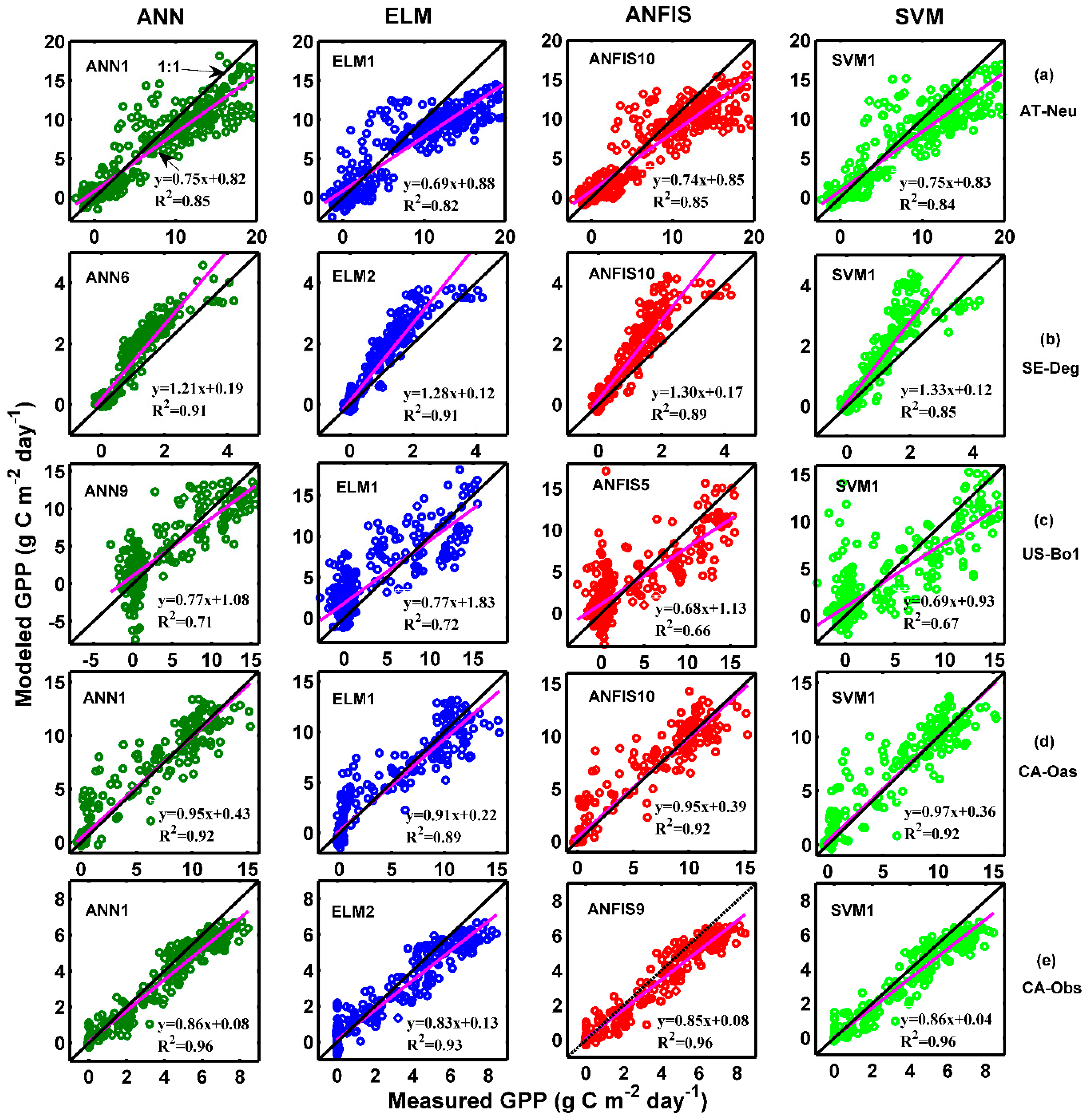
Figure 3.
Daily GPP observed via the eddy covariance method and modeled by the optimal machine learning models for the five sites in the whole period including training (the first four years), validation (the fifth year), and testing (the final year) periods. (a) ANN1 at AT-Neu; (b) ANN6 at SE-Deg; (c) ANN9 at US-Bo1; (d) ANFIS10 at CA-Oas; (e) ANN1 at CA-Obs.

Figure 4.
Model performance rankings of ecosystem respiration (R) estimation in the testing period: (a) for five different sites and four different machine learning methods with their respective internal functions (130 models); (b) for four different machine learning methods with their respective internal functions (26 models) at each site.
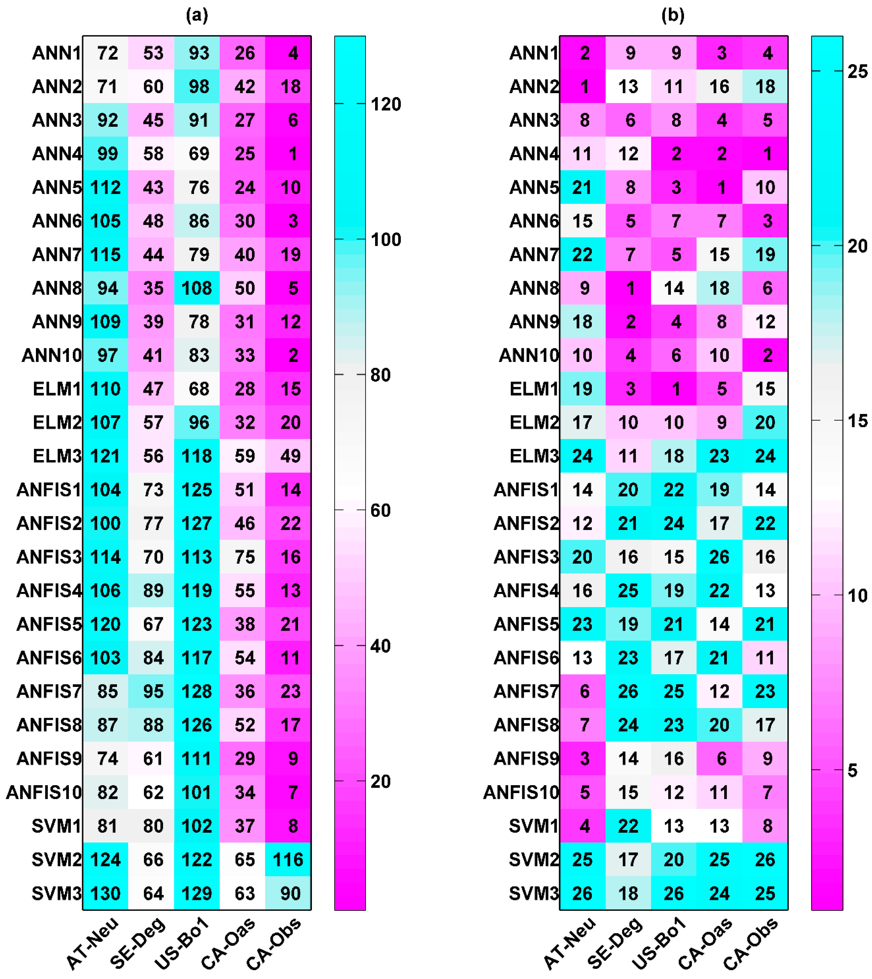
Figure 5.
Daily R values observed via the eddy covariance method and modeled by the four different machine learning models with the best internal functions in the testing period at the five sites. (a) AT-Neu; (b) SE-Deg; (c) US-Bo1; (d) CA-Oas; (e) CA-Obs.
Figure 5.
Daily R values observed via the eddy covariance method and modeled by the four different machine learning models with the best internal functions in the testing period at the five sites. (a) AT-Neu; (b) SE-Deg; (c) US-Bo1; (d) CA-Oas; (e) CA-Obs.
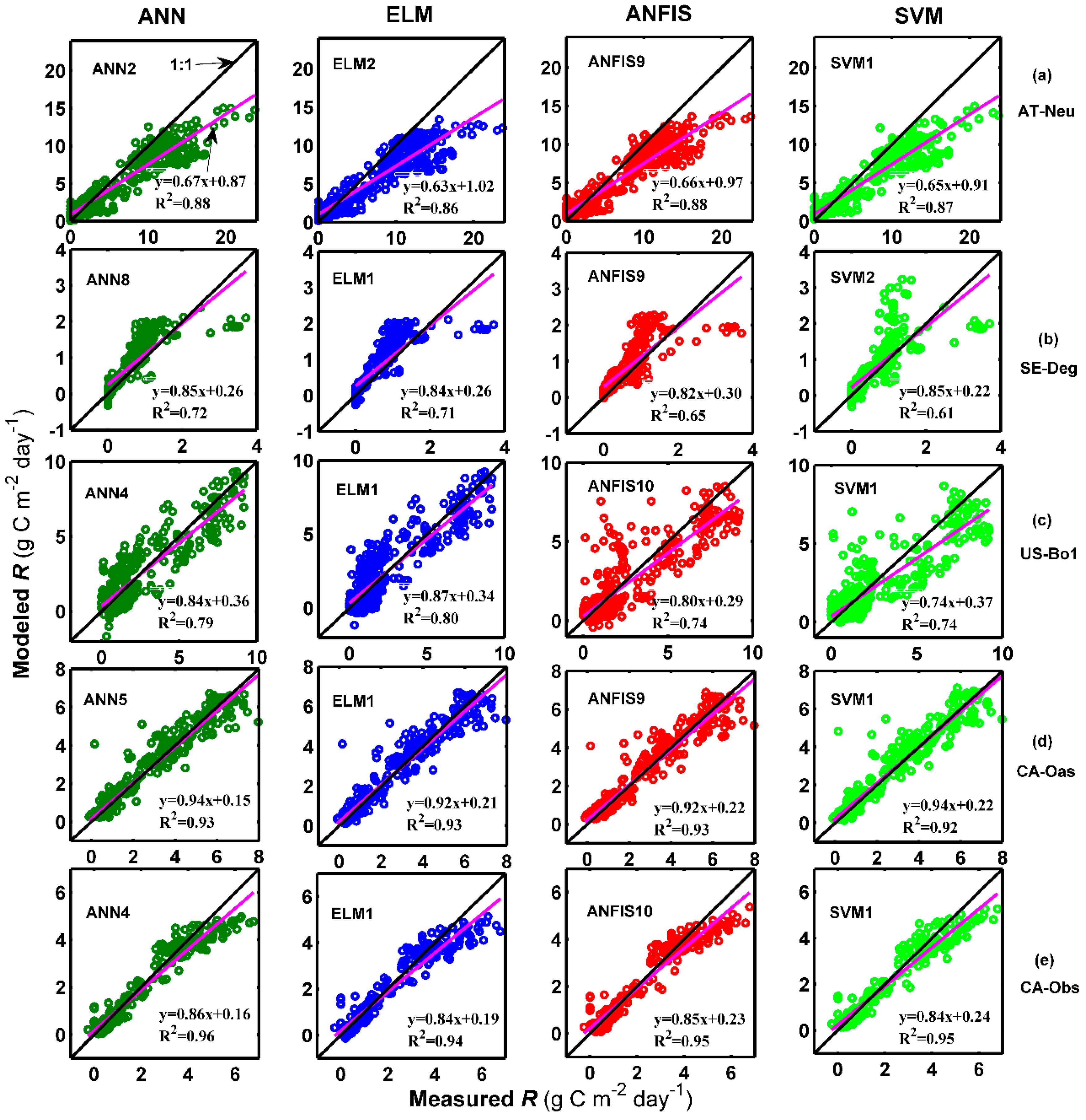
Figure 6.
Daily R observed via the eddy covariance method and modeled by the optimal machine learning models for the five sites in the whole period including training (the first four years), validation (the fifth year), and testing (the final year) periods. (a) ANN2 at AT-Neu; (b) ANN8 at SE-Deg; (c) ELM1 at US-Bo1; (d) ANN5 at CA-Oas; (e) ANN4 at CA-Obs.
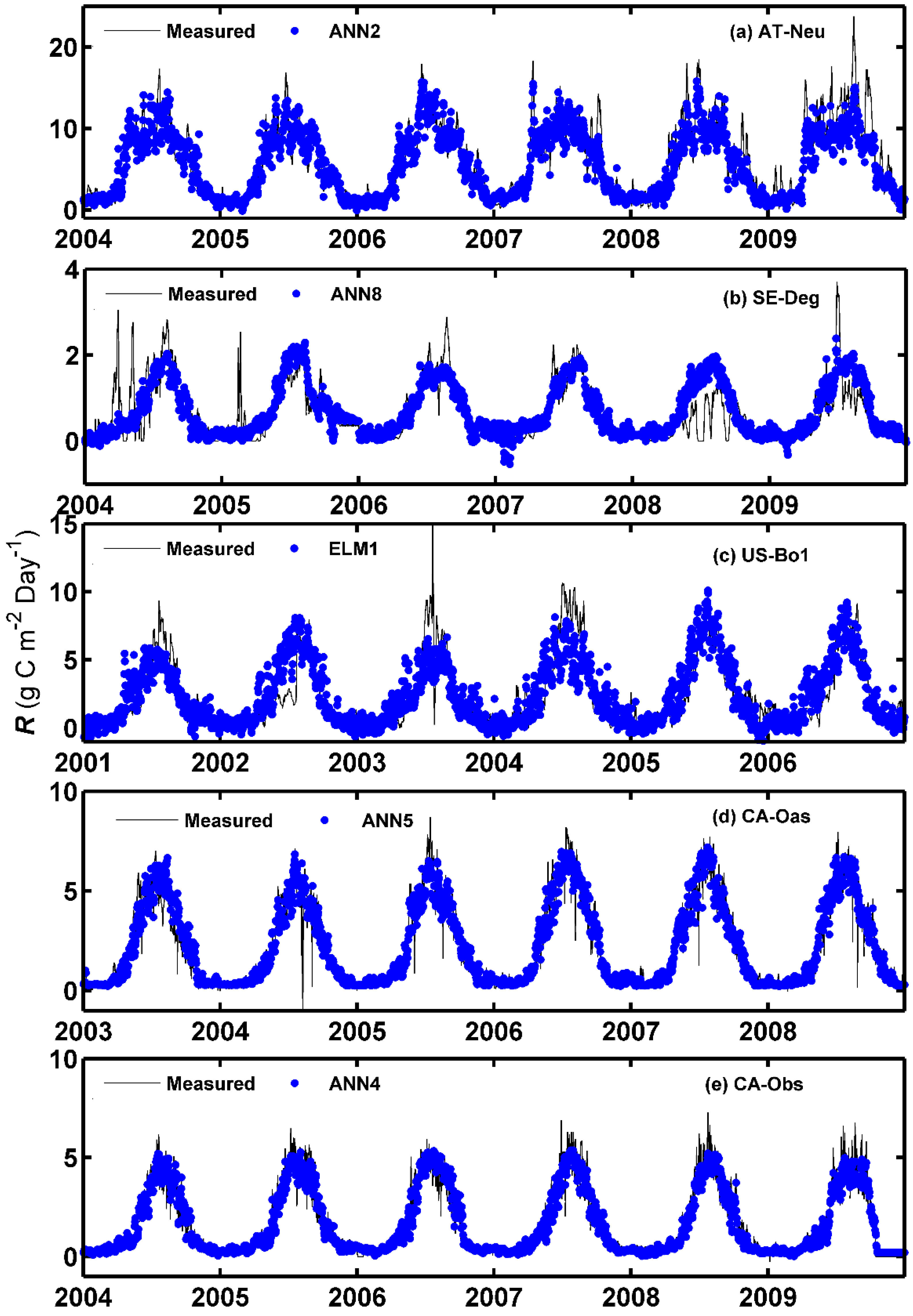
Figure 7.
Model performance rankings of net ecosystem exchange (NEE) estimation in the testing period: (a) for five different sites and four different machine learning methods with their respective internal functions (130 models); (b) for four different machine learning methods with their respective internal functions (26 models) at each site.
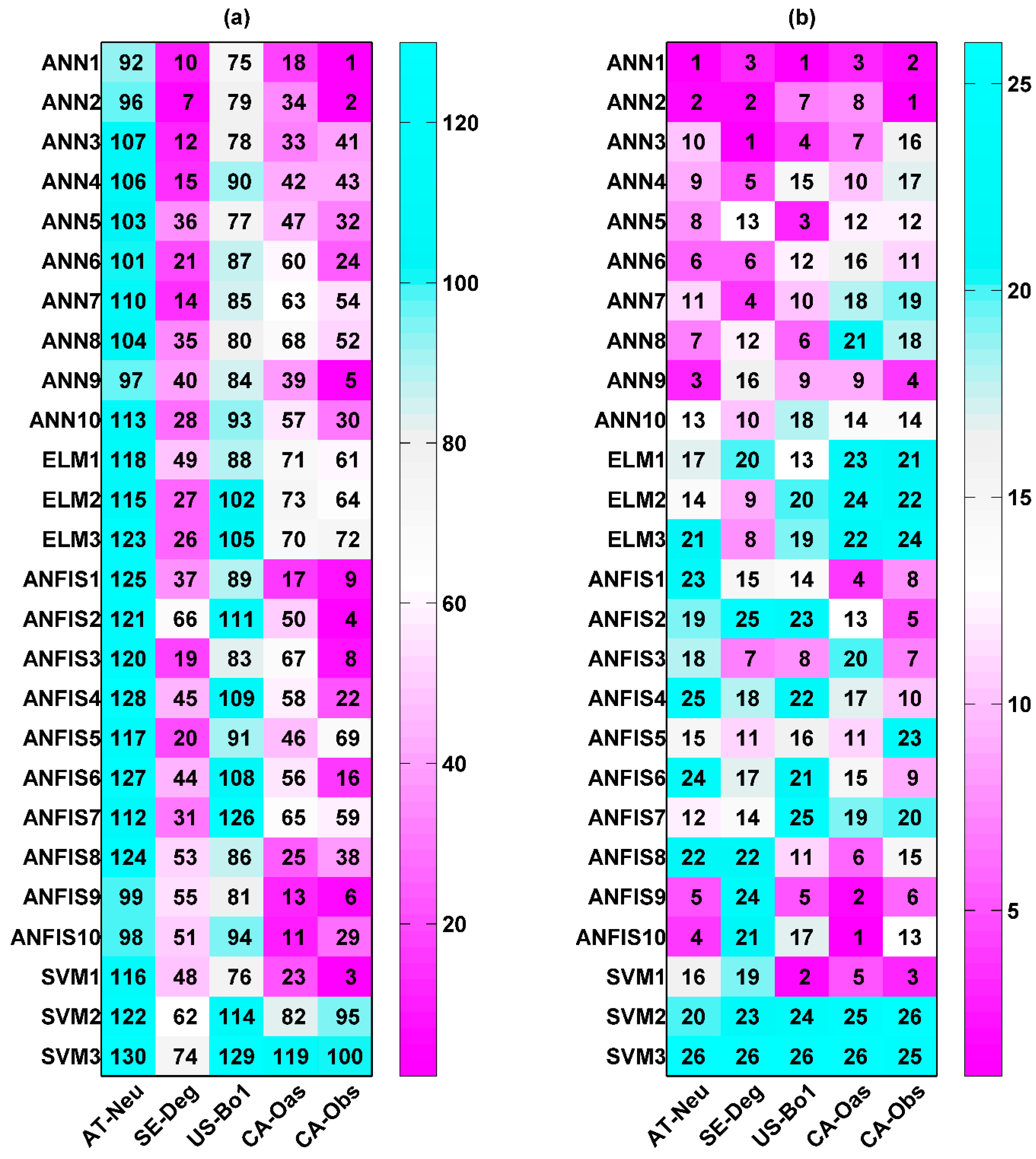
Figure 8.
Daily NEE observed via the eddy covariance method and modeled by the four different machine learning models with the best internal functions in the testing period at the five sites. (a) AT-Neu; (b) SE-Deg; (c) US-Bo1; (d) CA-Oas; (e) CA-Obs.
Figure 8.
Daily NEE observed via the eddy covariance method and modeled by the four different machine learning models with the best internal functions in the testing period at the five sites. (a) AT-Neu; (b) SE-Deg; (c) US-Bo1; (d) CA-Oas; (e) CA-Obs.

Figure 9.
Daily NEE observed via the eddy covariance method and modeled by the optimal machine learning models for the five sites in the whole period including training (the first four years), validation (the fifth year), and testing (the final year) periods. (a) ANN1 at AT-Neu; (b) ANN3 at SE-Deg; (c) ANN1 at US-Bo1; (d) ANFIS10 at CA-Oas; (e) ANN2 at CA-Obs.


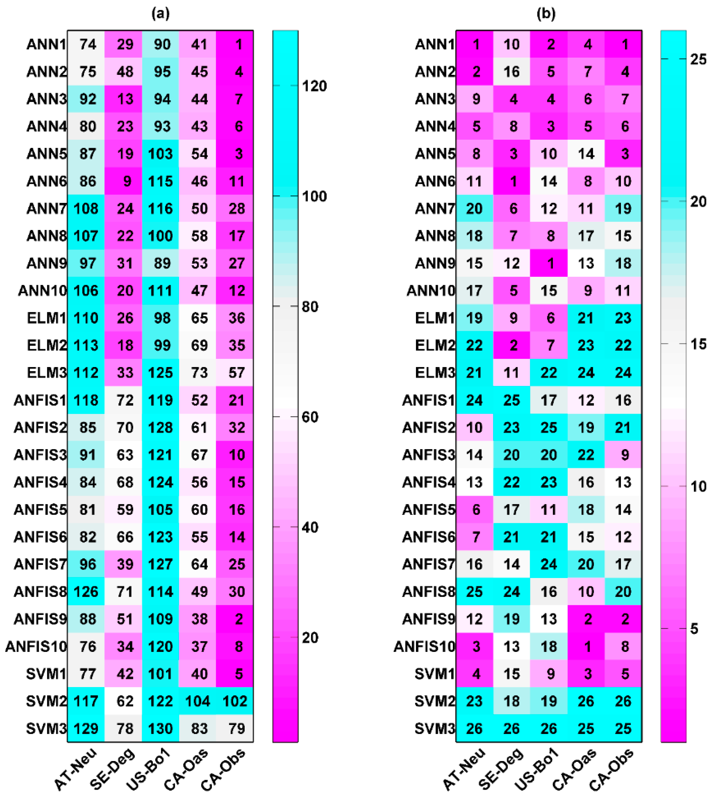
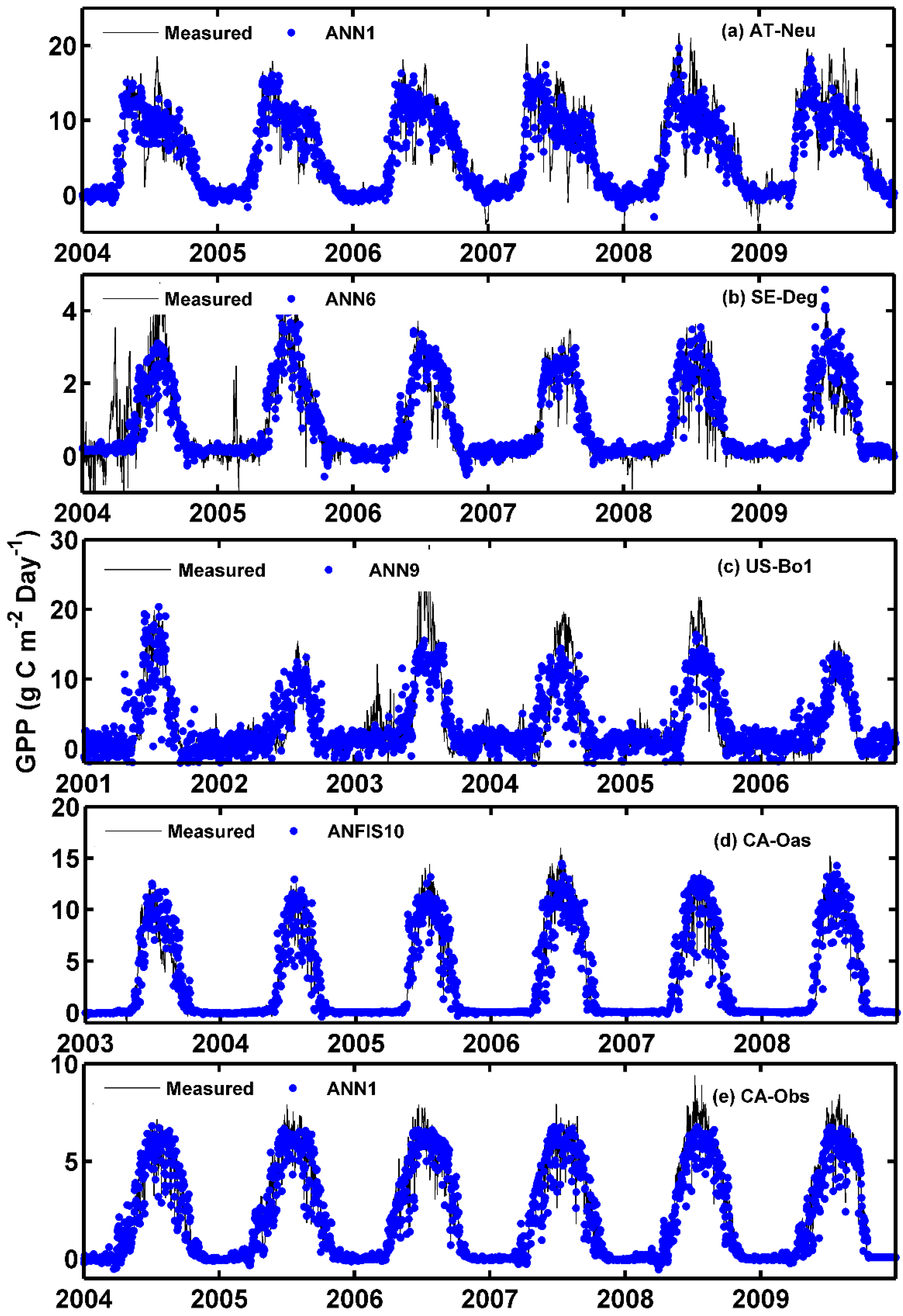
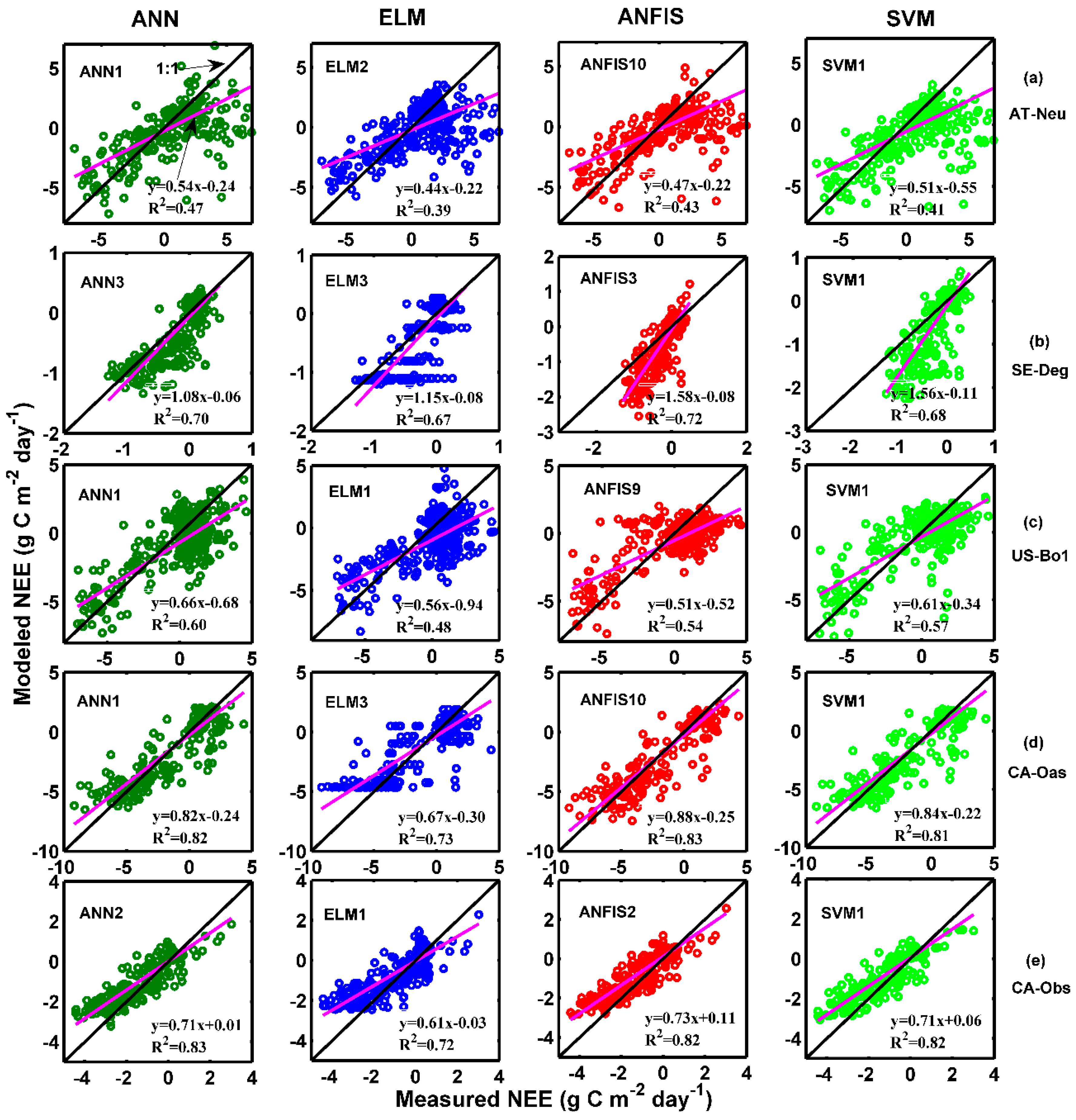
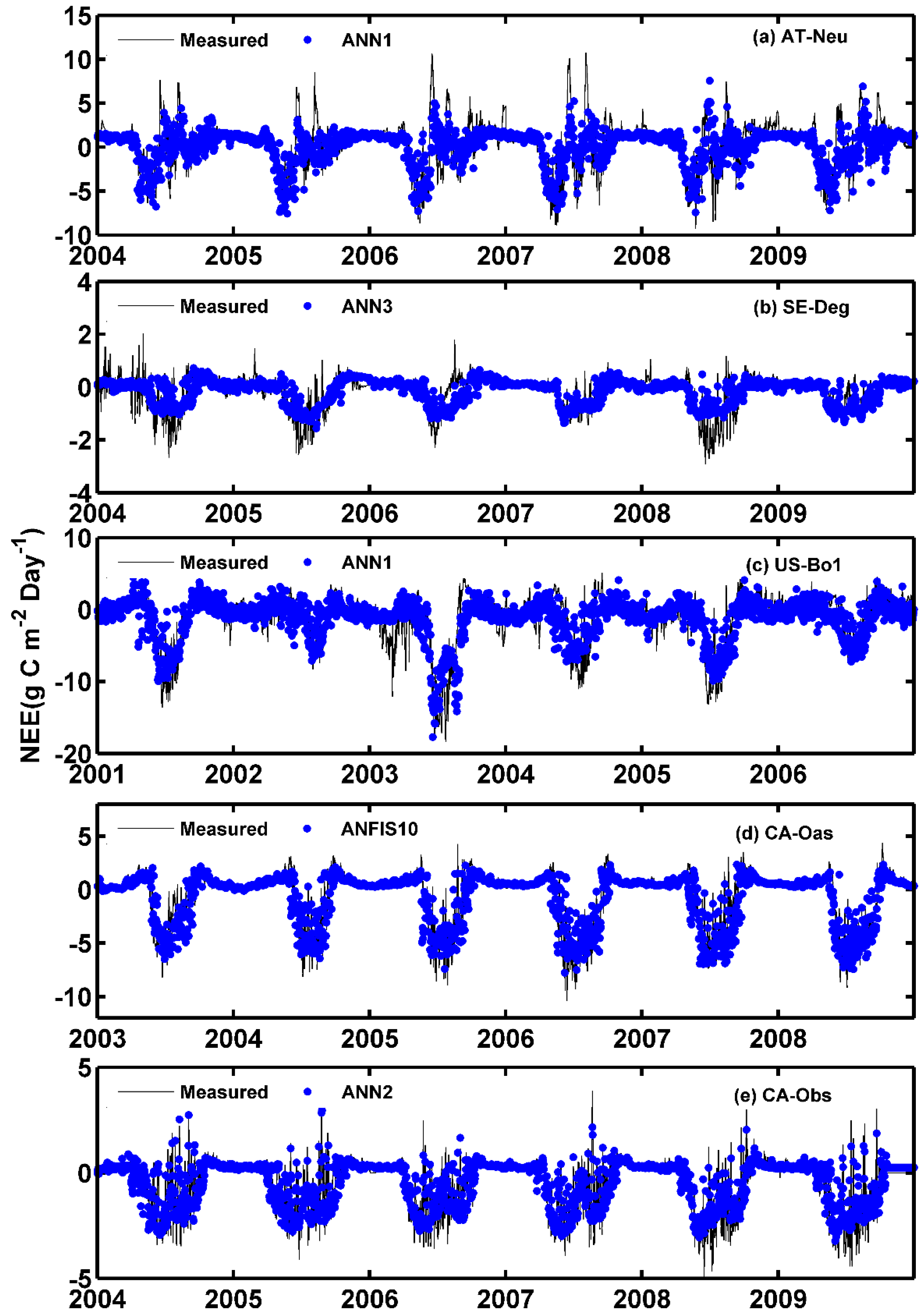
Table 1.
Site characteristics used in this study. The mean annual temperature (MAT, °C) and total annual precipitation (TAP, mm year−1) are calculated according to the time period (Period). Vegetation types include grassland (GRA), wetland (WET), cropland (CRO), deciduous broadleaf forest (DBF), and evergreen needle leaf forest (ENF).
| Site | Latitude | Longitude | Elevation | MAT | TAP | Vegetation | Period | Reference |
|---|---|---|---|---|---|---|---|---|
| AT-Neu | 47.12 | 11.32 | 970 | 6.68 | 669 | GRA | 2004–2009 | Wohlfahrt et al. [43] |
| SE-Deg | 64.18 | 19.55 | 270 | 2.90 | 436 | WET | 2004–2009 | Lund et al. [44] |
| US-Bo1 | 40.01 | −88.29 | 219 | 11.52 | 785 | CRO | 2001–2006 | Meyers and Hollinger [45] |
| CA-Oas | 53.63 | −106.20 | 601 | 1.82 | 343 | DBF | 2003–2008 | Griffis et al. [46] |
| CA-Obs | 53.99 | −105.12 | 629 | 1.00 | 373 | ENF | 2004–2009 | Krishnan et al. [47] |
Table 2.
Daily statistical parameters of eddy covariance tower measured environmental variables including air temperature (Ta, °C), net radiation (Rn, mol m−2), relative humidity (Rh, %), and soil temperature (Ts, °C) in the whole period in all five stands.
Table 2.
Daily statistical parameters of eddy covariance tower measured environmental variables including air temperature (Ta, °C), net radiation (Rn, mol m−2), relative humidity (Rh, %), and soil temperature (Ts, °C) in the whole period in all five stands.
| Stand | Variable | Xmean | Xmax | Xmin | Xsd | Xku | Xsk | CCGPP | CCR | CCNEE |
|---|---|---|---|---|---|---|---|---|---|---|
| AT-Neu | Ta | 6.68 | 22.96 | −17.63 | 8.19 | 2.24 | −0.29 | 0.80 | 0.88 | −0.23 |
| Rn | 4.24 | 16.51 | −6.44 | 5.33 | 1.97 | 0.16 | 0.81 | 0.77 | −0.43 | |
| Rh | 79.80 | 99.98 | 44.36 | 10.98 | 2.52 | −0.46 | −0.39 | −0.35 | 0.24 | |
| Ts | 8.71 | 21.28 | −2.56 | 6.86 | 1.50 | 0.01 | 0.81 | 0.88 | −0.24 | |
| SE-Deg | Ta | 2.90 | 28.40 | −26.79 | 9.43 | 2.90 | −0.08 | 0.77 | 0.74 | −0.54 |
| Rn | 2.43 | 14.72 | −12.74 | 4.33 | 2.41 | 0.54 | 0.67 | 0.50 | −0.62 | |
| Rh | 81.04 | 100.00 | 37.50 | 13.10 | 2.56 | −0.62 | −0.45 | −0.28 | 0.48 | |
| Ts | 4.98 | 16.75 | −0.31 | 4.99 | 1.89 | 0.61 | 0.79 | 0.73 | −0.59 | |
| US-Bo1 | Ta | 11.52 | 29.21 | −20.46 | 10.31 | 2.09 | −0.33 | 0.52 | 0.72 | −0.28 |
| Rn | 6.37 | 23.14 | −4.31 | 6.12 | 2.13 | 0.58 | 0.38 | 0.48 | −0.24 | |
| Rh | 74.80 | 100.00 | 17.98 | 17.46 | 3.60 | −0.97 | −0.01 | −0.02 | 0.01 | |
| Ts | 12.30 | 30.63 | −5.35 | 9.29 | 1.65 | 0.03 | 0.58 | 0.76 | −0.36 | |
| CA-Oas | Ta | 1.82 | 26.46 | −35.04 | 13.02 | 2.22 | −0.40 | 0.70 | 0.82 | −0.50 |
| Rn | 5.19 | 18.94 | −4.67 | 5.66 | 2.02 | 0.45 | 0.69 | 0.68 | −0.60 | |
| Rh | 69.88 | 98.78 | 21.83 | 16.15 | 2.62 | −0.52 | −0.18 | −0.21 | 0.13 | |
| Ts | 4.73 | 17.31 | −5.81 | 5.81 | 1.69 | 0.30 | 0.83 | 0.93 | −0.64 | |
| CA-Obs | Ta | 1.00 | 26.37 | −35.31 | 13.15 | 2.15 | −0.34 | 0.83 | 0.81 | −0.58 |
| Rn | 6.71 | 21.90 | −4.28 | 6.17 | 2.05 | 0.48 | 0.72 | 0.56 | −0.71 | |
| Rh | 72.35 | 100.00 | 24.56 | 16.69 | 2.46 | −0.43 | −0.31 | −0.16 | 0.42 | |
| Ts | 3.19 | 15.41 | −9.18 | 4.99 | 1.99 | 0.58 | 0.87 | 0.94 | −0.48 |
Note: Xmean, Xmax, Xmin, Xsd, Xku, and Xsk refer to the mean, maximum, minimum, standard deviation, kurtosis, and skewness of each variable, respectively; CCGPP, CCR, and CCNEE refer to the correlation coefficient between each variable and GPP, R, and NEE, respectively.
Table 3.
Performance of machine learning models with the best internal functions for gross primary productivity (GPP, g C m−2 day−1) among the training, validation, and testing periods in the five stands.
Table 3.
Performance of machine learning models with the best internal functions for gross primary productivity (GPP, g C m−2 day−1) among the training, validation, and testing periods in the five stands.
| Stand | Model | Training | Validation | Testing | |||||||||
|---|---|---|---|---|---|---|---|---|---|---|---|---|---|
| R2 | IA | RMSE | MAE | R2 | IA | RMSE | MAE | R2 | IA | RMSE | MAE | ||
| AT-Neu | ANN1 | 0.8312 | 0.9529 | 2.2268 | 1.4728 | 0.8529 | 0.9468 | 2.5424 | 1.9219 | 0.8519 | 0.9432 | 2.6885 | 1.9724 |
| ELM1 | 0.7760 | 0.9340 | 2.5641 | 1.7764 | 0.8225 | 0.9278 | 2.8483 | 2.1407 | 0.8201 | 0.9222 | 3.0660 | 2.3044 | |
| ANFIS10 | 0.8363 | 0.9540 | 2.1918 | 1.4487 | 0.8422 | 0.9398 | 2.6682 | 1.9318 | 0.8486 | 0.9412 | 2.7268 | 1.9568 | |
| SVM1 | 0.8377 | 0.9556 | 2.2129 | 1.3228 | 0.8349 | 0.9423 | 2.6402 | 1.9385 | 0.8433 | 0.9434 | 2.7004 | 1.9075 | |
| SE-Deg | ANN6 | 0.7951 | 0.9418 | 0.5184 | 0.3462 | 0.8303 | 0.9382 | 0.5019 | 0.3544 | 0.9140 | 0.9373 | 0.5116 | 0.3679 |
| ELM2 | 0.7952 | 0.9405 | 0.5175 | 0.3545 | 0.8204 | 0.9352 | 0.5352 | 0.3571 | 0.9059 | 0.9340 | 0.5389 | 0.3642 | |
| ANFIS10 | 0.8277 | 0.9512 | 0.4747 | 0.3181 | 0.8314 | 0.9297 | 0.5674 | 0.3803 | 0.8884 | 0.9158 | 0.6206 | 0.4122 | |
| SVM1 | 0.8743 | 0.9661 | 0.4068 | 0.2307 | 0.8310 | 0.9172 | 0.6543 | 0.4174 | 0.8483 | 0.9029 | 0.6782 | 0.4093 | |
| US-Bo1 | ANN9 | 0.6058 | 0.8653 | 3.6494 | 2.5147 | 0.7233 | 0.9074 | 3.1101 | 2.2727 | 0.7128 | 0.9127 | 2.5075 | 1.9127 |
| ELM1 | 0.4532 | 0.7804 | 4.2979 | 2.8972 | 0.8078 | 0.9459 | 2.6739 | 1.9537 | 0.7248 | 0.9017 | 2.6946 | 2.0094 | |
| ANFIS5 | 0.7113 | 0.9102 | 3.1227 | 2.0373 | 0.7606 | 0.9323 | 2.9541 | 2.0404 | 0.6582 | 0.8919 | 2.6830 | 1.8824 | |
| SVM1 | 0.6854 | 0.9024 | 3.2784 | 1.8555 | 0.7028 | 0.9099 | 3.2500 | 1.9768 | 0.6744 | 0.8984 | 2.6043 | 1.6394 | |
| CA-Oas | ANN1 | 0.9160 | 0.9778 | 1.2361 | 0.6850 | 0.9292 | 0.9775 | 1.2908 | 0.7781 | 0.9153 | 0.9771 | 1.3444 | 0.7653 |
| ELM1 | 0.8663 | 0.9630 | 1.5586 | 1.0494 | 0.8804 | 0.9663 | 1.5508 | 1.0379 | 0.8899 | 0.9707 | 1.4929 | 0.9629 | |
| ANFIS10 | 0.9124 | 0.9766 | 1.2618 | 0.6763 | 0.9329 | 0.9793 | 1.2326 | 0.7107 | 0.9189 | 0.9783 | 1.3044 | 0.6921 | |
| SVM1 | 0.9205 | 0.9792 | 1.2044 | 0.5942 | 0.9217 | 0.9750 | 1.3680 | 0.7567 | 0.9156 | 0.9772 | 1.3528 | 0.7324 | |
| CA-Obs | ANN1 | 0.9491 | 0.9868 | 0.5500 | 0.3633 | 0.9565 | 0.9779 | 0.7722 | 0.5063 | 0.9622 | 0.9836 | 0.6548 | 0.4220 |
| ELM2 | 0.9281 | 0.9810 | 0.6534 | 0.4868 | 0.9301 | 0.9710 | 0.8724 | 0.6255 | 0.9329 | 0.9741 | 0.8115 | 0.5682 | |
| ANFIS9 | 0.9484 | 0.9866 | 0.5535 | 0.3584 | 0.9531 | 0.9771 | 0.7875 | 0.5131 | 0.9595 | 0.9816 | 0.6898 | 0.4477 | |
| SVM1 | 0.9553 | 0.9884 | 0.5156 | 0.3091 | 0.9556 | 0.9778 | 0.7750 | 0.4936 | 0.9574 | 0.9818 | 0.6915 | 0.4290 | |
Table 4.
Performance of machine learning models with the best internal functions for ecosystem respiration (R, g C m−2 day−1) among the training, validation, and testing periods in the five stands.
Table 4.
Performance of machine learning models with the best internal functions for ecosystem respiration (R, g C m−2 day−1) among the training, validation, and testing periods in the five stands.
| Stand | Model | Training | Validation | Testing | |||||||||
|---|---|---|---|---|---|---|---|---|---|---|---|---|---|
| R2 | IA | RMSE | MAE | R2 | IA | RMSE | MAE | R2 | IA | RMSE | MAE | ||
| AT-Neu | ANN2 | 0.9035 | 0.9742 | 1.2858 | 0.9130 | 0.8853 | 0.9552 | 1.7460 | 1.2169 | 0.8834 | 0.9155 | 2.7290 | 1.9584 |
| ELM2 | 0.8708 | 0.9644 | 1.4878 | 1.0620 | 0.8807 | 0.9505 | 1.8119 | 1.2977 | 0.8590 | 0.8958 | 2.9793 | 2.1264 | |
| ANFIS9 | 0.8942 | 0.9714 | 1.3464 | 0.9579 | 0.8629 | 0.9543 | 1.8124 | 1.2480 | 0.8797 | 0.9122 | 2.7619 | 1.9803 | |
| SVM1 | 0.8988 | 0.9722 | 1.3205 | 0.8715 | 0.8702 | 0.9515 | 1.8184 | 1.2737 | 0.8708 | 0.9043 | 2.8800 | 2.0479 | |
| SE-Deg | ANN8 | 0.7031 | 0.9093 | 0.3765 | 0.2421 | 0.3091 | 0.6450 | 0.5947 | 0.3966 | 0.7212 | 0.9016 | 0.4011 | 0.2724 |
| ELM1 | 0.7028 | 0.9075 | 0.3763 | 0.2422 | 0.3078 | 0.6424 | 0.5948 | 0.3984 | 0.7096 | 0.8968 | 0.4107 | 0.2819 | |
| ANFIS9 | 0.7631 | 0.9294 | 0.3359 | 0.2123 | 0.3141 | 0.6478 | 0.5912 | 0.3806 | 0.6516 | 0.8709 | 0.4612 | 0.3253 | |
| SVM2 | 0.6525 | 0.8906 | 0.4142 | 0.2561 | 0.3679 | 0.6915 | 0.5484 | 0.3562 | 0.6098 | 0.8666 | 0.4776 | 0.2830 | |
| US-Bo1 | ANN4 | 0.6497 | 0.8828 | 1.5390 | 1.0309 | 0.8241 | 0.9519 | 1.0657 | 0.8351 | 0.7927 | 0.9419 | 1.1644 | 0.9524 |
| ELM1 | 0.6546 | 0.8852 | 1.5278 | 1.0300 | 0.8524 | 0.9545 | 1.1009 | 0.8443 | 0.7956 | 0.9437 | 1.1653 | 0.9155 | |
| ANFIS10 | 0.7939 | 0.9397 | 1.1800 | 0.7493 | 0.8338 | 0.9443 | 1.2617 | 0.9314 | 0.7415 | 0.9239 | 1.3215 | 0.9503 | |
| SVM1 | 0.8126 | 0.9454 | 1.1276 | 0.6244 | 0.7209 | 0.9169 | 1.3433 | 0.9443 | 0.7413 | 0.9175 | 1.3272 | 0.9492 | |
| CA-Oas | ANN5 | 0.9114 | 0.9765 | 0.6203 | 0.3824 | 0.9397 | 0.9845 | 0.5256 | 0.3594 | 0.9337 | 0.9827 | 0.5580 | 0.3580 |
| ELM1 | 0.9118 | 0.9765 | 0.6187 | 0.3740 | 0.9431 | 0.9852 | 0.5076 | 0.3340 | 0.9303 | 0.9815 | 0.5722 | 0.3595 | |
| ANFIS9 | 0.9238 | 0.9799 | 0.5751 | 0.3534 | 0.9287 | 0.9815 | 0.5714 | 0.3420 | 0.9299 | 0.9813 | 0.5741 | 0.3512 | |
| SVM1 | 0.9264 | 0.9808 | 0.5657 | 0.3039 | 0.9458 | 0.9858 | 0.5042 | 0.3319 | 0.9246 | 0.9800 | 0.6019 | 0.3701 | |
| CA-Obs | ANN4 | 0.9330 | 0.9824 | 0.4371 | 0.2818 | 0.9392 | 0.9791 | 0.4889 | 0.3273 | 0.9554 | 0.9845 | 0.4280 | 0.2944 |
| ELM1 | 0.9297 | 0.9815 | 0.4477 | 0.2874 | 0.9411 | 0.9798 | 0.4775 | 0.3061 | 0.9422 | 0.9800 | 0.4821 | 0.3289 | |
| ANFIS10 | 0.9391 | 0.9841 | 0.4167 | 0.2619 | 0.9418 | 0.9785 | 0.4902 | 0.3084 | 0.9498 | 0.9825 | 0.4522 | 0.3199 | |
| SVM1 | 0.9414 | 0.9847 | 0.4089 | 0.2334 | 0.9425 | 0.9791 | 0.4850 | 0.3102 | 0.9471 | 0.9809 | 0.4692 | 0.3385 | |
Table 5.
Performance of machine learning models with the best internal functions for net ecosystem exchange (NEE, g C m−2 day−1) among the training, validation, and testing periods in the five stands.
Table 5.
Performance of machine learning models with the best internal functions for net ecosystem exchange (NEE, g C m−2 day−1) among the training, validation, and testing periods in the five stands.
| Stand | Model | Training | Validation | Testing | |||||||||
|---|---|---|---|---|---|---|---|---|---|---|---|---|---|
| R2 | IA | RMSE | MAE | R2 | IA | RMSE | MAE | R2 | IA | RMSE | MAE | ||
| AT-Neu | ANN1 | 0.5032 | 0.8130 | 2.0021 | 1.2738 | 0.4827 | 0.8100 | 2.0669 | 1.4847 | 0.4679 | 0.8057 | 1.9879 | 1.2727 |
| ELM2 | 0.3843 | 0.7389 | 2.2282 | 1.4976 | 0.4798 | 0.7825 | 2.0855 | 1.6120 | 0.3862 | 0.7613 | 2.1270 | 1.4395 | |
| ANFIS10 | 0.4851 | 0.8038 | 2.0377 | 1.2949 | 0.6456 | 0.8543 | 1.7610 | 1.3050 | 0.4324 | 0.7789 | 2.0406 | 1.2892 | |
| SVM1 | 0.4781 | 0.8074 | 2.0784 | 1.1627 | 0.5855 | 0.8401 | 1.8886 | 1.3730 | 0.4099 | 0.7731 | 2.2073 | 1.3812 | |
| SE-Deg | ANN3 | 0.5493 | 0.8344 | 0.4267 | 0.2828 | 0.7219 | 0.8018 | 0.5597 | 0.3734 | 0.7018 | 0.8917 | 0.2638 | 0.1834 |
| ELM3 | 0.5437 | 0.8355 | 0.4278 | 0.2787 | 0.7171 | 0.8385 | 0.5307 | 0.3482 | 0.6747 | 0.8667 | 0.3080 | 0.2028 | |
| ANFIS3 | 0.7387 | 0.9203 | 0.3237 | 0.2123 | 0.7137 | 0.9131 | 0.4634 | 0.3016 | 0.7238 | 0.8147 | 0.4362 | 0.2693 | |
| SVM1 | 0.7619 | 0.9296 | 0.3091 | 0.1784 | 0.7067 | 0.9088 | 0.4686 | 0.2963 | 0.6800 | 0.7910 | 0.4685 | 0.2736 | |
| US-Bo1 | ANN1 | 0.5440 | 0.8411 | 2.6355 | 1.8241 | 0.6539 | 0.8699 | 2.3804 | 1.7979 | 0.5999 | 0.8579 | 1.6549 | 1.3337 |
| ELM1 | 0.3628 | 0.7179 | 3.1072 | 2.2364 | 0.6812 | 0.8863 | 2.2871 | 1.7946 | 0.4836 | 0.7931 | 1.9581 | 1.6110 | |
| ANFIS9 | 0.5789 | 0.8530 | 2.5261 | 1.7290 | 0.2906 | 0.6814 | 3.4383 | 2.2186 | 0.5387 | 0.8179 | 1.6927 | 1.3535 | |
| SVM1 | 0.5572 | 0.8497 | 2.6103 | 1.5559 | 0.6013 | 0.8676 | 2.5591 | 1.7161 | 0.5679 | 0.8523 | 1.6019 | 1.1772 | |
| CA-Oas | ANN1 | 0.7755 | 0.9313 | 1.2105 | 0.7227 | 0.7561 | 0.9267 | 1.2592 | 0.7873 | 0.8163 | 0.9471 | 1.1252 | 0.6872 |
| ELM3 | 0.6380 | 0.8797 | 1.5348 | 1.0086 | 0.6994 | 0.9011 | 1.3719 | 0.9026 | 0.7293 | 0.9087 | 1.3745 | 0.8726 | |
| ANFIS10 | 0.7935 | 0.9397 | 1.1591 | 0.6545 | 0.8044 | 0.9394 | 1.2147 | 0.7318 | 0.8345 | 0.9540 | 1.0826 | 0.6343 | |
| SVM1 | 0.7867 | 0.9369 | 1.1783 | 0.6314 | 0.7765 | 0.9343 | 1.2225 | 0.7280 | 0.8125 | 0.9474 | 1.1390 | 0.6518 | |
| CA-Obs | ANN2 | 0.8083 | 0.9441 | 0.5080 | 0.3407 | 0.8496 | 0.9389 | 0.6095 | 0.4113 | 0.8292 | 0.9306 | 0.6165 | 0.4407 |
| ELM1 | 0.6754 | 0.8956 | 0.6610 | 0.4944 | 0.7611 | 0.8831 | 0.7850 | 0.5716 | 0.7216 | 0.8827 | 0.7651 | 0.5640 | |
| ANFIS2 | 0.8108 | 0.9454 | 0.5045 | 0.3345 | 0.8584 | 0.9369 | 0.6169 | 0.4184 | 0.8224 | 0.9237 | 0.6560 | 0.5027 | |
| SVM1 | 0.8130 | 0.9457 | 0.5019 | 0.3139 | 0.8406 | 0.9320 | 0.6358 | 0.4313 | 0.8175 | 0.9255 | 0.6426 | 0.4746 | |
© 2018 by the authors. Licensee MDPI, Basel, Switzerland. This article is an open access article distributed under the terms and conditions of the Creative Commons Attribution (CC BY) license (http://creativecommons.org/licenses/by/4.0/).
Share and Cite
MDPI and ACS Style
Dou, X.; Yang, Y. Comprehensive Evaluation of Machine Learning Techniques for Estimating the Responses of Carbon Fluxes to Climatic Forces in Different Terrestrial Ecosystems. Atmosphere 2018, 9, 83. https://doi.org/10.3390/atmos9030083
AMA Style
Dou X, Yang Y. Comprehensive Evaluation of Machine Learning Techniques for Estimating the Responses of Carbon Fluxes to Climatic Forces in Different Terrestrial Ecosystems. Atmosphere. 2018; 9(3):83. https://doi.org/10.3390/atmos9030083
Chicago/Turabian StyleDou, Xianming, and Yongguo Yang. 2018. "Comprehensive Evaluation of Machine Learning Techniques for Estimating the Responses of Carbon Fluxes to Climatic Forces in Different Terrestrial Ecosystems" Atmosphere 9, no. 3: 83. https://doi.org/10.3390/atmos9030083
Note that from the first issue of 2016, this journal uses article numbers instead of page numbers. See further details here.