Article

On-Road Air Quality Associated with Traffic Composition and Street-Canyon Ventilation: Mobile Monitoring and CFD Modeling

1
School of Natural Resources and Environmental Science, Kangwon National University, Chuncheon 24341, Korea
2
Center for Environment, Health and Welfare Research, Korea Institute of Science and Technology, Seoul 02792, Korea
3
Center for Particulate Air Pollution and Health, Korea Institute of Science and Technology, Seoul 02792, Korea
4
Department of Environmental Engineering, Konkuk University, Seoul 05029, Korea
5
School of Earth and Environmental Sciences, Seoul National University, Seoul 08826, Korea
*
Author to whom correspondence should be addressed.
Atmosphere 2018, 9(3), 92; https://doi.org/10.3390/atmos9030092
Submission received: 1 February 2018 / Revised: 24 February 2018 / Accepted: 24 February 2018 / Published: 2 March 2018
(This article belongs to the Special Issue Recent Advances in Urban Ventilation Assessment and Flow Modelling)

Abstract

:
Mobile monitoring and computational fluid dynamics (CFD) modeling are complementary methods to examine spatio-temporal variations of air pollutant concentrations at high resolutions in urban areas. We measured nitrogen oxides (NOx), black carbon (BC), particle-bound polycyclic aromatic hydrocarbons (pPAH), and particle number (PN) concentrations in a central business district using a mobile laboratory. The analysis of correlations between the measured concentrations and traffic volumes demonstrate that high emitting vehicles (HEVs) are deterministically responsible for poor air quality in the street canyon. The determination coefficient (R2) with the HEV traffic volume is the largest for the pPAH concentration (0.79). The measured NOx and pPAH concentrations at a signalized intersection are higher than those on a road between two intersections by 24% and 25%, respectively. The CFD modeling results reveal that the signalized intersection plays a role in increasing on-road concentrations due to accelerating and idling vehicles (i.e., emission process), but also plays a countervailing role in decreasing on-road concentrations due to lateral ventilation of emitted pollutants (i.e., dispersion process). It is suggested that the number of HEVs and street-canyon ventilation, especially near a signalized intersection, need to be controlled to mitigate poor air quality in a central business district of a megacity.

Graphical Abstract

1. Introduction

Vehicle emission is one of the major sources of air pollution in urban areas. Exposure to air pollutants that are emitted from vehicles can cause human health problems, such as cardiovascular, respiratory, and allergic diseases [1,2,3]. Diesel exhaust was recently classified as Group 1 carcinogen by the International Agency for Research on Cancer [4].
On-road emissions of primary pollutants (e.g., nitrogen oxides (NOx = NO + NO2), carbon monoxide (CO), and particulate matter) have been estimated based on nationwide annual databases and are allocated with specified temporal and spatial profiles. In estimating on-road emissions, an emission factor or emission rate of air pollutant is calculated using various factors. Across a nation, the number of registered vehicles, traffic volume and composition, fuel-use fraction, and vehicle age are well reported. For example, on-road emission studies have stated that heavy-duty diesel vehicles (HDDVs), or heavy emitters, dominantly contribute up to 50% of NO2, 41% of NOx, 51% of CO, 77% of black carbon (BC), 70% of polycyclic aromatic hydrocarbons (PAHs), 50% of particle number (PN), and 60% of particulate matter emissions [5,6,7,8,9,10]. It is challenging to represent the effects of actual driving situations on on-road emissions because driving mode (i.e., idling, accelerating, cruising, and decelerating) and road configuration (i.e., intersection, upslope, and downslope) spatio-temporally vary at small scale, particularly in urban areas [11,12]. Among various driving situations, congestion with frequent accelerations at low vehicle speeds [13,14,15], signalized traffic intersection [16,17], and upslope [7,18] are found to aggravate on-road air quality.
Intra-urban variability of on-road air quality is largely associated with not only vehicle emission distribution [19,20], but also urban built environment [21,22,23]. A street canyon is a space that is enclosed by road and roadside buildings on both sides and is often characterized by heavy traffic, poor ventilation, and a large floating population. The street canyon has attracted many researchers for pollutant emission and dispersion studies because of the direct impacts on human health and the excellence as an experimental space similar to a road tunnel. To investigate the distribution of near-or on-road air quality, mobile measurements have been utilized to overcome certain limitations to the representation of spatial variability when using stationary measurements [24,25,26,27,28,29]. A few studies using mobile measurements have focused on the street-canyon environment in the central business districts of New York City [30], Hong Kong [31], Seoul [32], and Thessaloniki [33], where situations are highly complex. The first aim of this study is to investigate on-road air quality in a street canyon in a central business district using a mobile laboratory (ML) and the relationship between the on-road air quality and individual traffic compositions that are heavily responsible for pollutant emissions.
Air quality in the street canyon is significantly influenced by dispersion characteristics due to in-canyon ventilation along with ambient wind as well as vehicle emission [34,35]. To take the dispersion characteristics into account suitably, numerical models have been utilized to examine on-road emission and dispersion in the urban built environment [36,37,38,39,40]. Computational fluid dynamics (CFD) models can explicitly resolve roads and buildings at high resolutions [41,42,43]. Mobile monitoring and CFD modeling are complementary methods to examine the temporal and spatial patterns of air quality in street canyons. CFD modeling requires a real-world pollutant emission rate on roads as a boundary condition for any pollutant concentration, while mobile monitoring results need to be interpreted by considering pollutant dispersion with the presence of building and ambient wind effects. The second aim of this study is to investigate the horizontal distribution of on-road air quality in a street canyon in a central business district by applying CFD modeling results for analyzing mobile monitoring results.

2. Methods

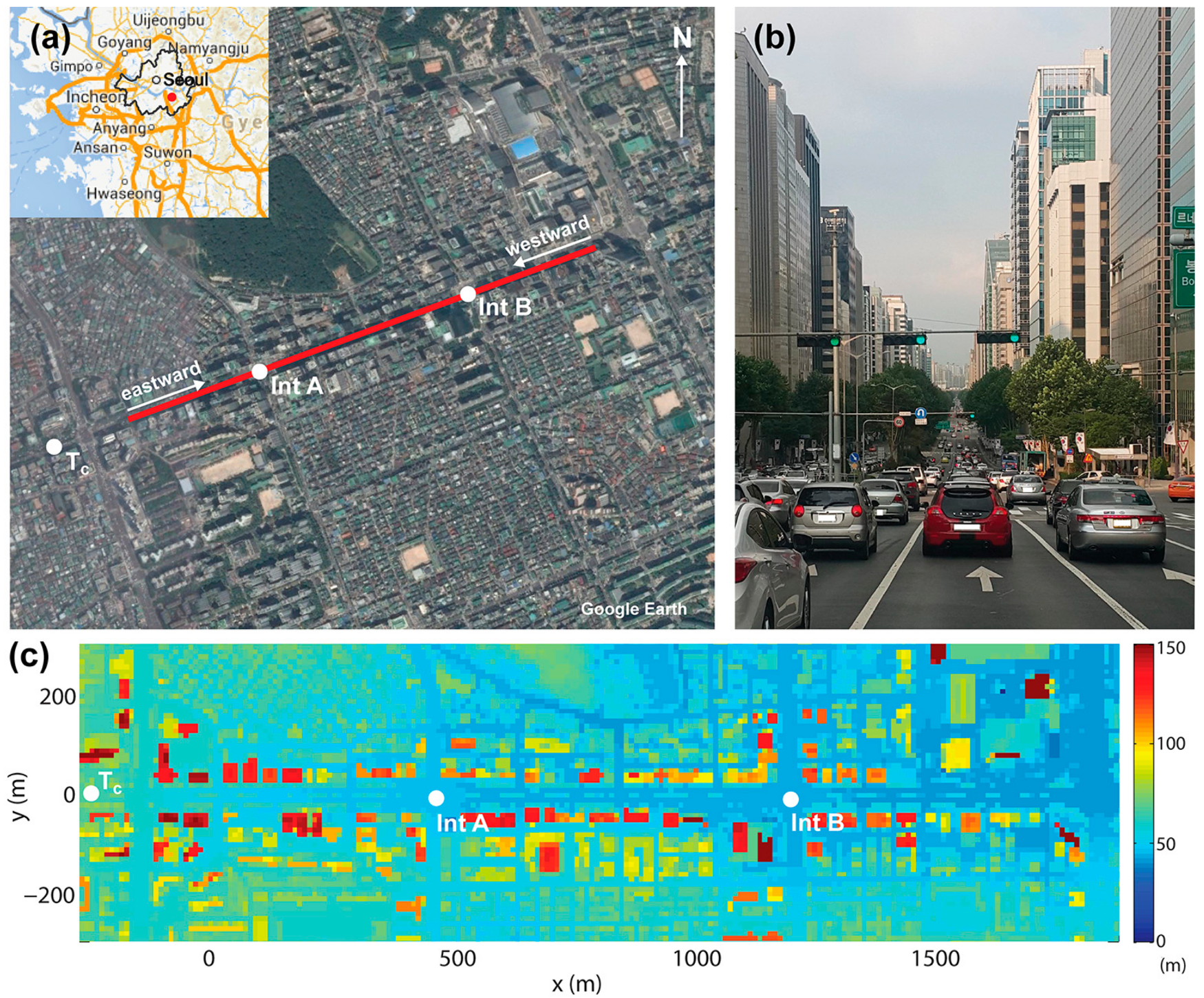
2.1. Site Description

The study area of interest is a street canyon of eight-lane Teheran road with a southwest-northeast (i.e., 249° and 69° from the due north) orientation in a central business district of Seoul, which is a megacity in Republic of Korea (Figure 1a). The areas surrounding Teheran road are highly-developed commercial and residential areas, and a vegetated area is located in the north. Many high-rise buildings are densely located on both sides in the 1.8 km-long street canyon crossing with four-lane and six-lane roads at signalized intersections A and B, respectively (Figure 1b,c). The elevation of road gradually decreases from the southwest to the northeast by a few meters.
The traffic volumes of private cars, taxis, RV/SUVs, trucks, vans, buses, and motorcycles were manually counted at Tc. At first, traffic flows on the road were continuously recorded using a video camera in a roadside building for a week. Then, the number of vehicles in each traffic composition was counted for 15 min consecutively. Note that diesel and gasoline vehicles were not distinguished during this process. The diurnal variations of hourly traffic volumes on 5–8 November 2013 are shown in Figure 2. The traffic pattern on Teheran road is different from the typical bimodal pattern with maxima during the morning and evening rush-hours in urban areas. The daily traffic volume is over 90,000 vehicles on weekdays, and the maximum hourly traffic volume appears in the middle of working hours (i.e., 11:00–12:00 LT). The hourly traffic volume larger than 4000 vehicles consistently appears from 08:00 to 23:00 LT. Among the seven traffic compositions, private car (50%) accounts for the largest portion of traffic volume followed by taxi (28%), RV/SUV (9%), and truck (4%). Here, RV/SUVs, trucks, vans, and buses are grouped into high emitting vehicles (HEVs) based on their conventional vehicle emissions. The daily HEV traffic volume is 19% of the daily total traffic volume. The HEV portion of hourly traffic volume reaches a maximum during the morning rush hour (07:00–08:00 LT) (29%) and remains larger than 20% (06:00–17:00 LT) till the working hours.

2.2. Mobile Monitoring

The mobile monitoring was repeatedly conducted in the 1.8 km-long street canyon of Teheran road on 5–8 November 2013 (Table 1). During the three monitoring periods, the predominant wind directions were the along-canyon direction (period 1), opposite along-canyon direction (period 2), and direction oblique to along-canyon direction (period 3). An ML has been developed and operated for the last few years to monitor on-road concentrations of gaseous and particulate air pollutants in urban areas [16,32]. The sampling inlet in front of the ML at a 2-m height consists of a Teflon tube and a stainless steel pipe for gaseous and particulate pollutants, respectively. Table 2 provides the brief information on the instruments equipped in the ML. NOx, BC, particle-bound PAH (pPAH), and PN (>5 nm) concentrations were measured using a chemiluminescence NOx analyzer (AC32M, Environmental S.A., Poissy, France), an aethalometer (AE42, Magee Scientific, Berkeley, CA, USA) with an impactor of 2.5 μm cut-off diameter, a photoelectric aerosol sensor (PAS2000, EcoChem Analytics, League City, TX, USA), and a condensation particle counter (CPC model 5.403, GRIMM, Ainring, Germany), respectively. In the pre-processing step, the NOx analyzer was calibrated using pure air and standard NO gas, and the instruments for particulate pollutants were initialized and/or zero checked. The time in the data acquisition system was synchronized with the global positioning system (GPS) data that was recorded every 1 s by a GPS data logger (GPS742, Ascen, Seoul, Republic of Korea). In the post-processing step, delay times of instruments in the ML were adjusted.
The on-road measurements of NOx, BC, pPAH, and PN concentrations during the three periods are divided into every two-way trip starting from the eastern end of the street canyon. Thirteen trips for each period are valid after excluding incomplete and interrupted measurements. In every trip, the median concentration is calculated in every 100-m section in the street canyon for each driving direction. A 100-m spacing is acceptable for studying the spatial variation of air pollutant near a major road [44]. For calculating the median concentration in a 100-m section, the measured concentrations with a vehicle speed higher than 20 km h−1 are used to avoid the effects of exhaust plumes of a vehicle directly ahead [45].

2.3. CFD Modeling

The CFD model used in this study is a Reynolds-averaged Navier–Stokes equations (RANS) model with the renormalization group (RNG) k-ε turbulence closure scheme [46]. The RANS model has been validated and used for simulating urban flow and pollutant dispersion, particularly in street canyons [43,47,48]. Numerical simulations are performed for the three dispersion scenarios corresponding to mobile monitoring periods 1, 2, and 3. The isothermal condition is considered because of sufficiently low air temperature (7–17 °C) and reduced or absent daylight during the mobile monitoring periods. The size of the domain covering the 1.8-km long street canyon oriented in the x-direction and surrounding commercial and residential areas is 4000 m in the x-direction, 1800 m in the y-direction, and 997 m in the z-direction. The grid size is 10 m in the x- and y-direction and 4 m in the z-direction up to z = 200 m, with an increasing ratio (1.05) of vertical grid size above the height. The surface geometries in the domain were obtained from the airborne light detection and ranging (LIDAR) measurement (Figure 1c). The logarithmic vertical wind profile is applied at the inflow boundaries. Inflow wind speed at the top boundary (z = 997 m) and direction are 1.4 m s−1 and 69° from the due north for the period-1 scenario, 1.7 m s−1 and 249° from the due north for the period-2 scenario, and 2.0 m s−1 and 292° from the due north for the period-3 scenario. A zero-gradient boundary condition is applied at the outflow boundaries. At all of the boundaries, the vertical velocity is specified to be zero. The inflow pollutant concentration is set to zero, and the inert pollutant emission is identically considered at a same emission rate for all the lowest grids on major roads (the number of lanes ≥ 2) in the domain. As the vertical size of lowest grids on roads is 4 m, it is accordingly assumed that the emitted pollutants at the tailpipe are instantaneously mixed by the vehicle-induced turbulence within the extents of grids. On Teheran road, four rows of grids corresponding to the 40-m width in the y-direction are considered to be the pollutant emission points. It is noteworthy that the emission setting is deviated from the real-world emission distribution in order to solely examine the dispersion of emitted pollutants on roads in different dispersion scenarios. The model integration time is 120 min, with a time step of 1 s. Pollutant emission is activated after 10-min integration.

3. Results and Discussion

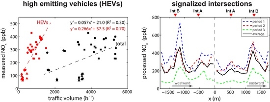
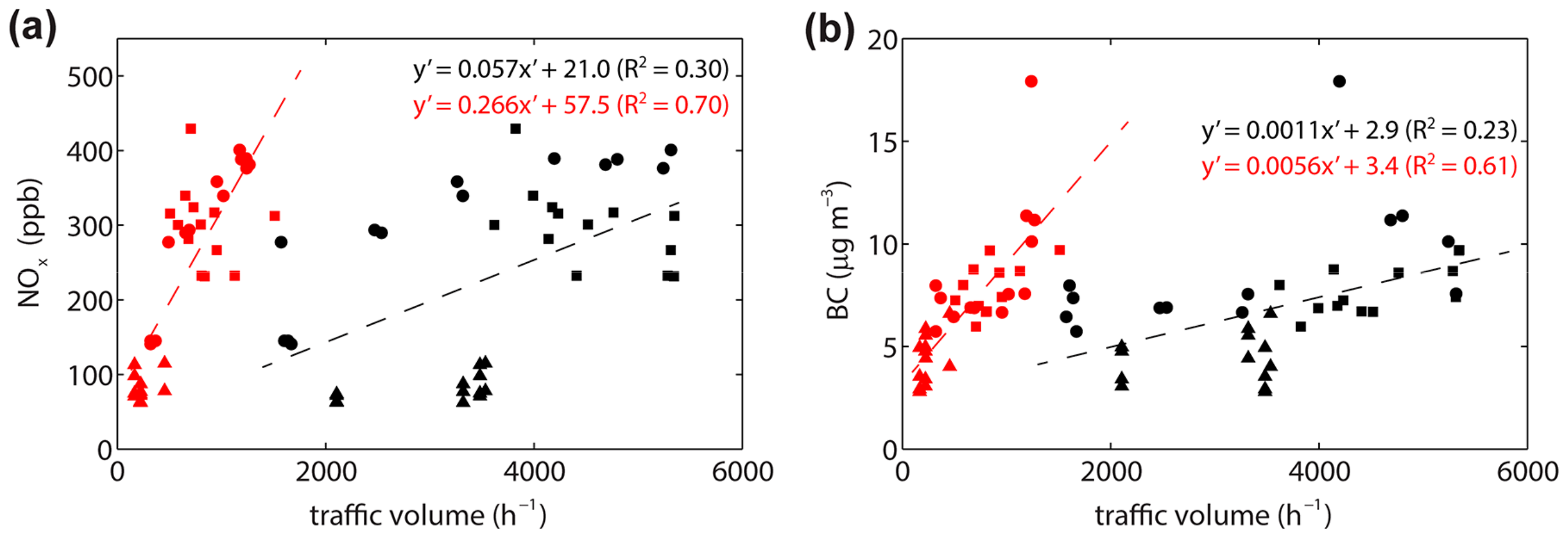
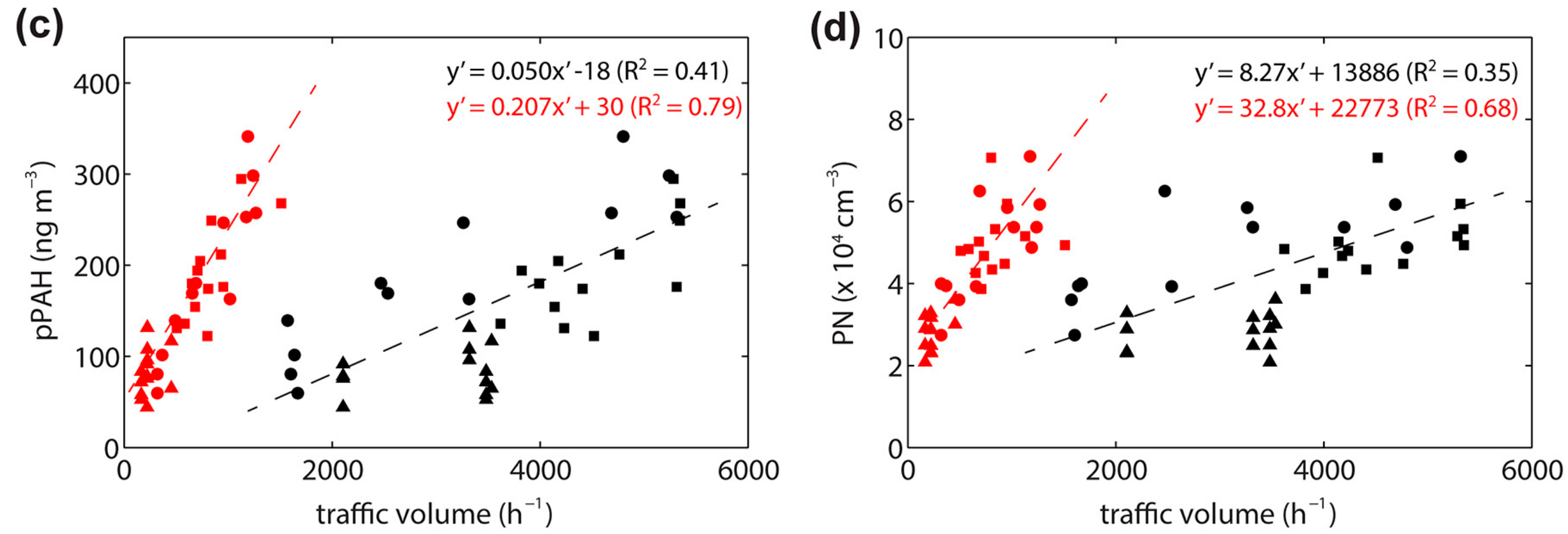
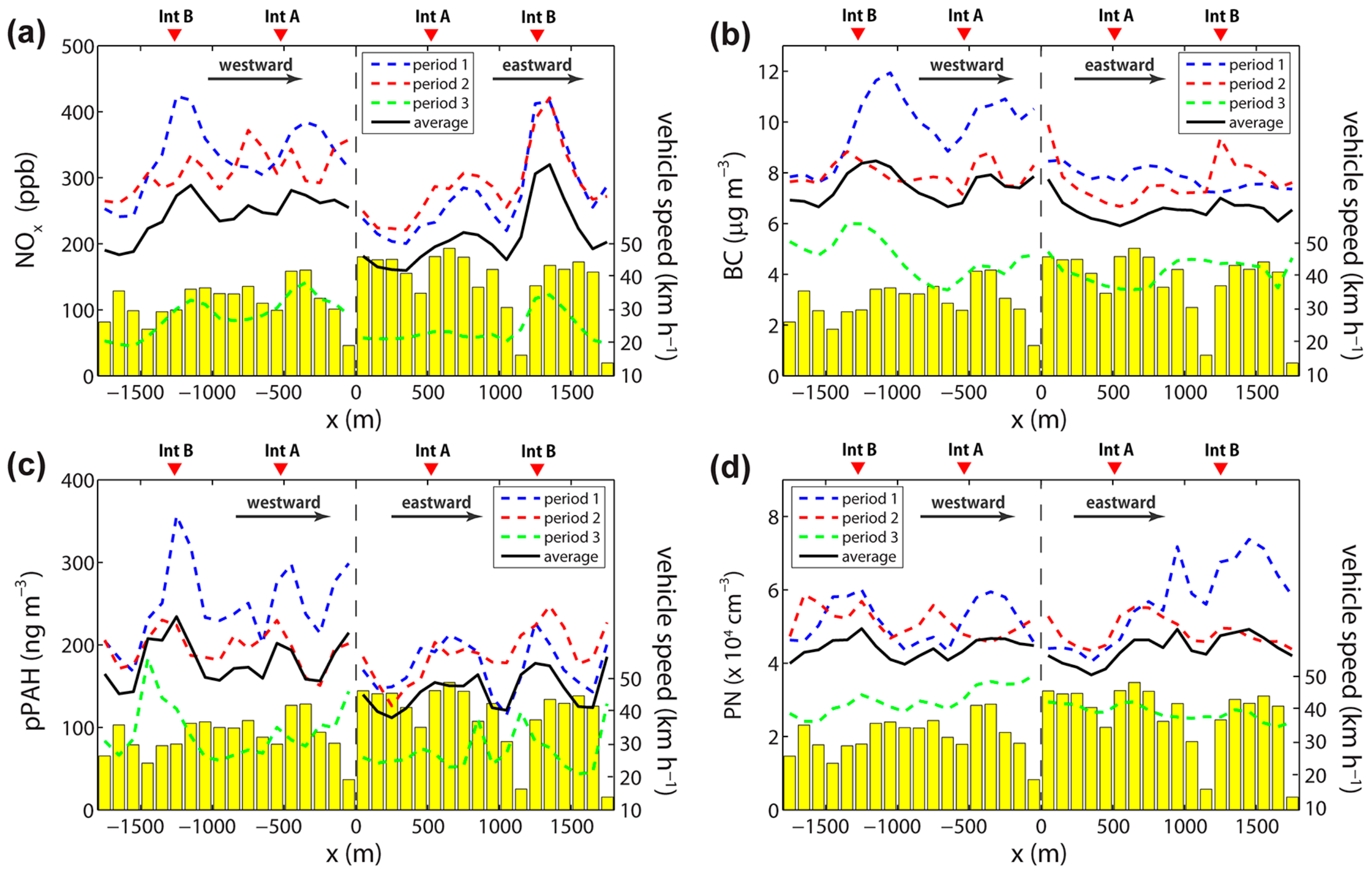
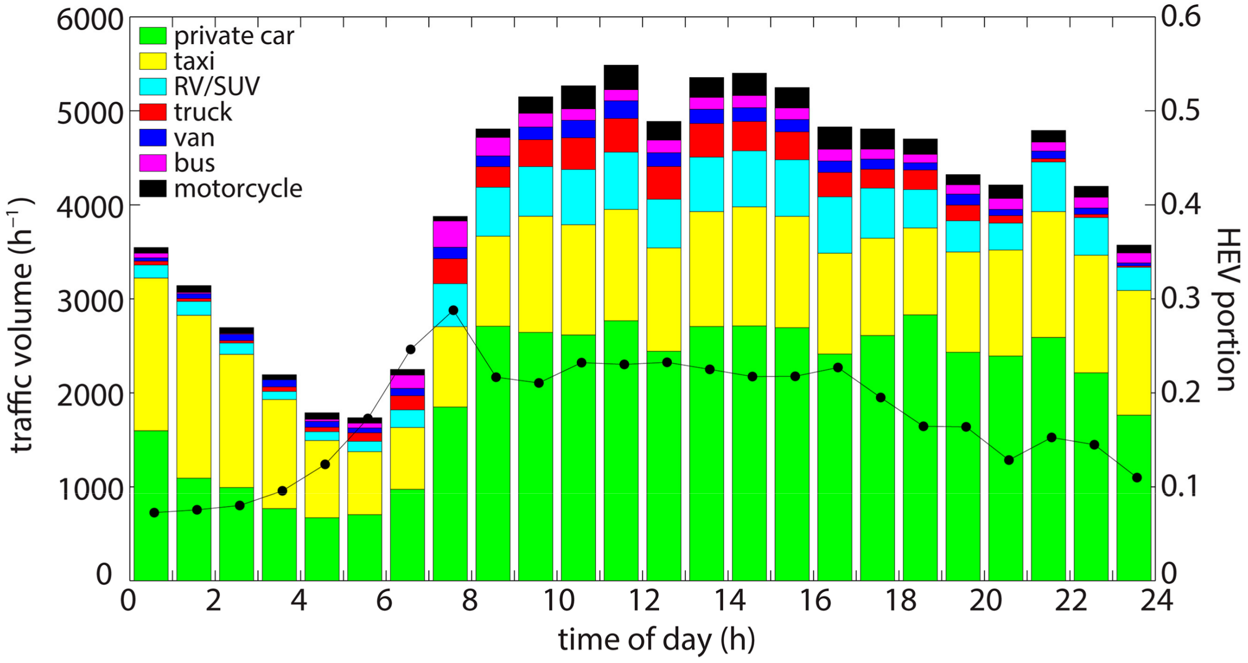
3.1. Association with Traffic Composition

The measured NOx, BC, pPAH, and PN concentration for a trip is obtained by averaging their median concentrations of all 100-m sections. Similar to the concentrations, the traffic volumes collected for 15 min consecutively during the mobile monitoring periods are assigned to the corresponding trips. Then, the traffic volumes of each composition are averaged for each trip. The associations of the measured concentrations with the traffic volumes of individual compositions are analyzed by calculating the determination coefficients (R2) based on the linear regressions for 39 trips in the street canyon (Table 3). Although private car has the largest portion of traffic volumes, the correlations with the NOx, BC, pPAH, and PN concentrations are intermediate (0.36, 0.26, 0.41, and 0.42, respectively). Taxi has the second largest portion of traffic volumes and is more weakly correlated with the concentrations than private car. This is because the majority of private car and taxi are gasoline-and liquefied petroleum gas (LPG)-powered vehicles, respectively. In contrast to private car and taxi, RV/SUV for which the portion of traffic volumes is only 9% is strongly correlated with the NOx, BC, pPAH, and PN concentrations (R2 = 0.52, 0.44, 0.62, and 0.44, respectively). The emission amount of a RV/SUV is undoubtedly smaller than that of a truck, van, or bus. However, the 2–4 times larger traffic volume of RV/SUV than those of truck, van, and bus results in stronger or similar correlations with the concentrations. The first and second largest determination coefficients among the seven traffic compositions for any measured pollutant correspond to one of the HEV compositions (i.e., RV/SUV, truck, van, or bus). It is thought that the on-road emission capacities of individual compositions grouped into HEVs are comparable to each other and obviously larger than those of private car, taxi, and motorcycle in the street canyon.
The scatter diagrams (Figure 3) exhibit that the measured NOx, BC, pPAH, and PN concentrations are well correlated with the traffic volumes. Among the measured pollutants, the highest correlations with the traffic volumes are shown for the pPAH concentration (R2 = 0.41 and 0.79 for the total and HEV traffic volumes, respectively), whereas the lowest ones are shown for the BC concentration (R2 = 0.23 and 0.61 for the total and HEV traffic volumes, respectively). The highest correlations for the pPAH concentration are attributed to the dominant contribution of local mobile sources to the concentration in a roadside environment [49]. Regardless of pollutants, the correlations with the HEV traffic volume are significantly higher than those with the total traffic volume. This implies that only 19% of the total traffic volume is capable of describing the on-road pollutant concentrations in the street canyon. The relative importance of HEVs to the on-road pollutant concentrations is assessed with the linear regression lines in the scatter diagrams. When the pollutant concentration is ideally correlated with the traffic volume, the slope and y-intercept of a regression line indicate an increase in concentration per an increase in traffic volume and a base concentration with no vehicle emission on a road, respectively. The slopes of the regression lines for the HEV traffic volume are distinctly 4–5 times larger than those for the total traffic volume. The increase in concentration responding to the increase in HEV traffic volume is 266 ppb for NOx, 5.6 μg m−3 for BC, 207 ng m−3 for pPAH, and 3.28 × 104 cm−3 for PN per 1000 HEVs. Although the increase in concentration is not entirely attributed to the HEV emission, the concentration gradient with respect to the HEV traffic volume can be a useful indicator to the on-road NOx, BC, pPAH, and PN concentrations in the street canyon.

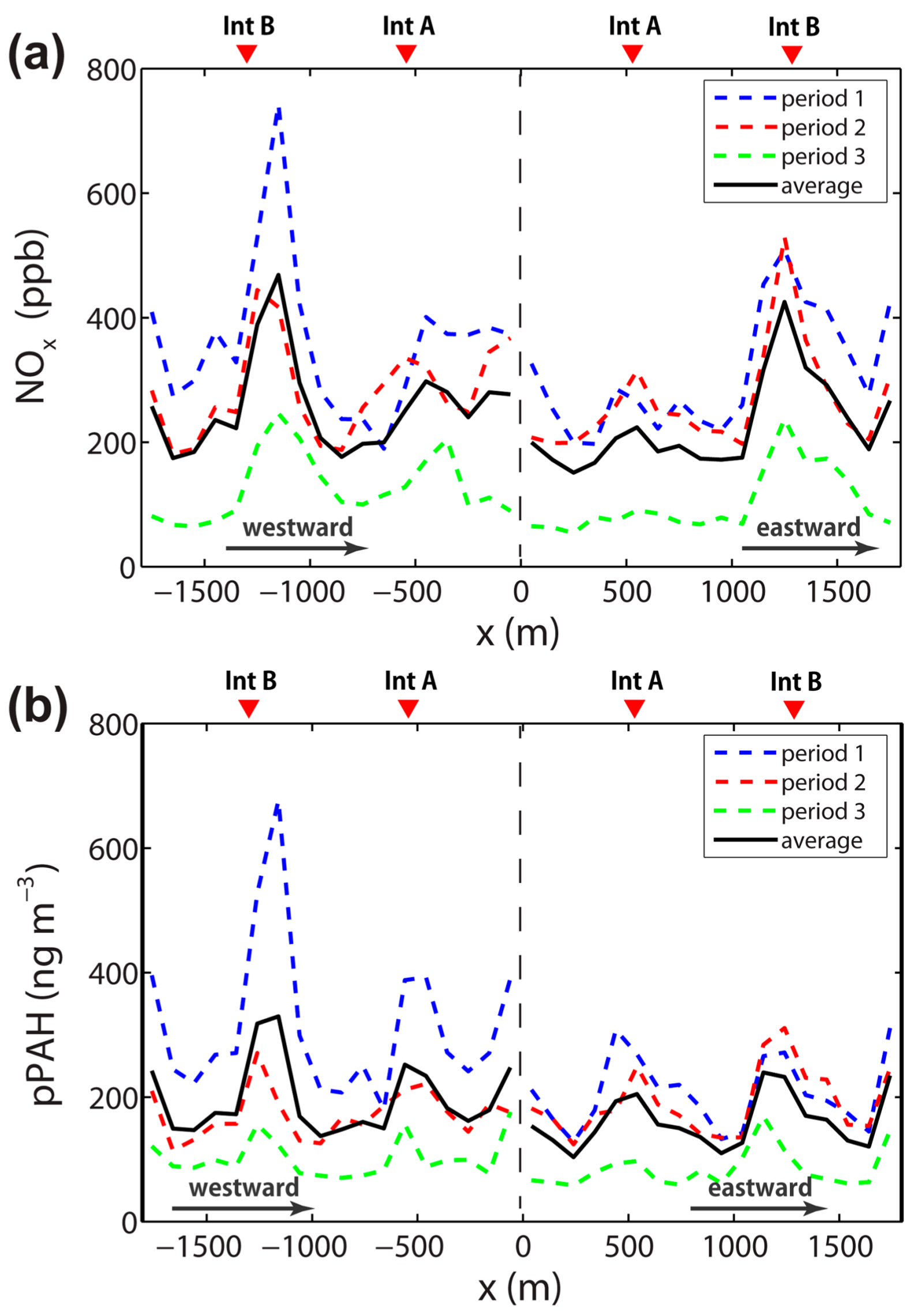
3.2. Association with Street-Canyon Ventilation

The measured NOx, BC, pPAH, and PN concentrations are unevenly distributed in the 1.8-km street canyon. The unevenly distributed concentrations in the street canyon are attributed to the combination of uneven driving modes due to traffic signals and congestion and irregular street-canyon ventilation. In the following analysis, the distributions of measured concentrations in the street canyon are presented first and later converted by taking account of the influence of pollutant dispersion through CFD model simulations for the three dispersion scenarios.
Figure 4 shows the horizontal distributions of measured NOx, BC, pPAH, and PN concentrations and ML speed in the street canyon. The median NOx, BC, pPAH, and PN concentrations and ML speed in 100-m sections for 13 trips are averaged over each mobile monitoring period. Among the three periods, all of the measured concentrations in 100-m sections are the lowest for period 3 (i.e., nighttime) when the traffic volume is the smallest. The average NOx, BC, and pPAH concentrations that were measured during the westward driving are generally higher than those that were measured during the eastward driving. This is because of slight upsloping and also congested traffic flow in the westward driving direction. The average PN concentrations tend to be invariable, regardless of driving direction. The NOx and pPAH concentrations at the two signalized intersections are higher than those between the intersections by up to 24% and 25%, respectively (Table 4). The higher NOx and pPAH concentrations are more significant at signalized intersection B than at signalized intersection A. This is because vehicle emissions are larger at signalized intersection B due to accelerating and idling vehicles, not only on Teheran road, but also on the six-lane road that perpendicularly cross with the street canyon. The differences between concentrations at the intersections and those between the intersections for BC and PN are smaller (<±10%) than those for NOx and pPAH (Table 4). The y-intercepts of linear regression lines for HEV traffic volumes in Figure 3 may explain the base NOx, BC, pPAH, and PN concentrations (57.5 ppb, 3.4 μg m−3, 30 ng m−3, and 22,773 cm−3, respectively). The NOx and pPAH concentrations at the intersections are 4–6 times higher than the base concentrations, while BC and PN concentrations at the intersections are only about two times higher than the base concentrations. The BC and PN concentrations are less localized than the NOx and pPAH concentrations at the signalized intersections partly because the time resolution for the BC measurement is relatively large, and also because some influencing sources outside other than HEVs are considerably involved in determining on-road BC and PN concentrations.
Scalar dispersion for the three different scenarios corresponding to mobile monitoring periods 1, 2, and 3 is numerically examined through the CFD model simulations with an identical distribution of on-road pollutant emission. Scalar dispersion has been commonly interpreted as dispersion of chemically inactive gases or ultrafine particles at small scale such as road environment [50]. Figure 5 shows the horizontal distributions of normalized on-road wind speed and pollutant concentration (hereafter, model coefficient) and of building height on the driving side in the street canyon for the three dispersion scenarios. The on-road wind speeds are normalized by the ambient (inflow) wind speed for each simulation. On the other hand, the on-road concentrations are normalized by the average on-road concentration over the three simulations. By doing this, the influence of ambient wind direction is included in both horizontal distributions of normalized on-road wind speeds and concentrations, whereas the influence of ambient wind speed is solely included in the horizontal distribution of normalized on-road concentrations. Therefore, the average of all the model coefficients for the three simulations is unity. The normalized on-road wind speed is generally higher for the period-1 and period-2 dispersion scenarios than for the period-3 dispersion scenario, since the ambient wind directions are fairly parallel to the canyon orientation for the period-1 and period-2 dispersion scenarios. The higher on-road wind speed for the parallel ambient wind directions is attributed to channeling flows that formed in the street canyon [51,52]. However, the normalized on-road pollutant concentration is higher for the period-1 and period-2 dispersion scenarios than for the period-3 dispersion scenario. This is because the emitted pollutants hardly escape from the street canyon for the parallel ambient wind directions. The ambient wind speed is slightly lower during periods 1 and 2 than during period 3, which also contributes to the inverse-proportional increase in on-road pollutant concentration. As a result, the ambient wind direction as well as the ambient wind speed is one of the determining factors in estimating the on-road pollutant concentrations in the street canyon. The normalized on-road wind speed is obviously high at the intersections where roadside buildings rarely obstruct lateral ventilation. The normalized on-road pollutant concentrations are consequently low at the intersections, particularly at intersection B wider than intersection A.
It is interesting that emission and dispersion processes play counterbalancing roles in determining any pollutant concentration at a signalized intersection in the street canyon. At a signalized intersection, pollutants are intensively emitted from idling and accelerating vehicles and are ventilated out of the street canyon. Figure 6 exhibits the horizontal distributions of converted NOx and pPAH concentrations in the street canyon. The converted concentration is the measured concentration (shown in Figure 4) multiplied by a reciprocal of the model coefficient (shown in Figure 5b). In the process, the influence of pollutant dispersion is excluded from the measured concentration. In the calculation of converted concentrations, the BC and PN concentrations are not taken into account because their base concentrations seem to be comparable to their on-road concentrations. The horizontal variations of converted NOx and pPAH concentrations become more pronounced since the converted NOx and pPAH concentrations are elevated at intersections A and B. The converted NOx and pPAH concentrations are higher than those between the intersections by 7% and 26% at signalized intersection A, respectively, and by 57% and 43% at signalized intersection B, respectively (Table 4). The higher converted concentrations than the measured concentrations are more evident at signalized intersection B than at signalized intersection A. This reveals that signalized intersection B is a distinct hotspot where the dispersion process acts to alleviate severe air pollution due to the emission process. In conclusion, the emission process aggravates on-road air quality in the street canyon, and is efficiently compensated by the dispersion process at signalized intersection B. Later, the horizontal distributions of converted NOx and pPAH concentrations can be utilized as the real-world on-road emission for realistic CFD modeling.

4. Conclusions

Spatio-temporal variations of air pollutant concentrations in a street canyon in a central business district of Seoul, Republic of Korea were investigated on multiple days based on complementary approaches using an ML and a CFD model. The ML monitored primary pollutants that were emitted from on-road vehicles, and traffic volume and composition were recorded at the same time. The CFD model simulates pollutant dispersion in the presence of proper inflow boundary conditions and real building morphology. In the emission and dispersion processes of on-road air pollutants, the HEV portion and the street-canyon ventilation are the determining factors of the spatio-temporal variations in their on-road concentrations. Among the seven traffic compositions, RV/SUV appears to be the most responsible for poor air quality in the street canyon. A signalized intersection that is commonly characterized as a traffic hotspot exhibits countervailing roles between the emission and dispersion processes. In the street canyon, air quality at a signalized intersection is aggravated by up to 25% over that between signalized intersections due to the emission increase that is partially compensated by efficient lateral ventilation. Consequently, controlling the number of HEVs and the in-canyon ventilation near signalized intersections can effectively manage on-road air quality in street canyons.

Acknowledgments

This work was supported by the Korea Auto-Oil Program (13-04-10) and the Institutional Program (2E28160) of the Korea Institute of Science and Technology.

Author Contributions

Kyung-Hwan Kwak conducted CFD modeling and wrote the paper; Sung Ho Woo, Kyung Hwan Kim, and Seung-Bok Lee conducted mobile monitoring; Seung-Bok Lee and Gwi-Nam Bae managed the research project and contributed to the discussion of mobile monitoring results; Young-Il Ma and Young Sunwoo analyzed the traffic data; Jong-Jin Baik contributed to CFD modeling.

Conflicts of Interest

The authors declare no conflict of interest.

References

  1. Bernard, S.M.; Samet, J.M.; Grambsch, A.; Ebi, K.L.; Romieu, I. The potential impacts of climate variability and change on air pollution-related health effects in the United States. Environ. Health Perspect. 2001, 109, 199–209. [Google Scholar] [CrossRef] [PubMed]
  2. Kim, B.-J.; Lee, S.-Y.; Kwon, J.-W.; Jung, Y.-H.; Lee, E.; Yang, S.I.; Kim, H.-Y.; Seo, J.-H.; Kim, H.-B.; Kim, H.-C.; et al. Traffic-related air pollution is associated with airway hyperresponsiveness. J. Allergy Clin. Immunol. 2014, 133, 1763–1765. [Google Scholar] [CrossRef] [PubMed]
  3. Halonen, J.I.; Blangiardo, M.; Toledano, M.B.; Fecht, D.; Gulliver, J.; Anderson, H.R.; Beevers, S.D.; Dajnak, D.; Kelly, F.J.; Tonne, C. Long-term exposure to traffic pollution and hospital admissions in London. Environ. Pollut. 2016, 208, 48–57. [Google Scholar] [CrossRef] [PubMed]
  4. IARC. Diesel Engine Exhaust Carcinogenic; International Agency for Research on Cancer, World Health Organization: Lyon, France, 2012; Available online: http://www.iarc.fr/en/media-centre/pr/2012/pdfs/pr213_E.pdf (accessed on 1 March 2018).
  5. Riddle, S.G.; Robert, M.A.; Jakober, C.A.; Hannigan, M.P.; Kleeman, M.J. Size-resolved source apportionment of airborne particle mass in a roadside environment. Environ. Sci. Technol. 2008, 42, 6580–6586. [Google Scholar] [CrossRef] [PubMed]
  6. Wang, X.; Westerdahl, D.; Wu, Y.; Pan, X.; Zhang, K.M. On-road emission factor distributions of individual diesel vehicles in and around Beijing, China. Atmos. Environ. 2011, 45, 503–513. [Google Scholar] [CrossRef]
  7. Wang, X.; Westerdahl, D.; Hu, J.; Wu, Y.; Yin, H.; Pan, X.; Zhang, K.M. On-road diesel vehicle emission factors for nitrogen oxides and black carbon in two Chinese cities. Atmos. Environ. 2012, 46, 45–55. [Google Scholar] [CrossRef]
  8. Dallmann, T.R.; DeMartini, S.J.; Kirchstetter, T.W.; Herndon, S.C.; Onasch, T.B.; Wood, E.C.; Harley, R.A. On-road measurement of gas and particle phase pollutant emission factors for individual heavy-duty diesel trucks. Environ. Sci. Technol. 2012, 46, 8511–8518. [Google Scholar] [CrossRef] [PubMed]
  9. Tan, Y.; Lipsky, E.M.; Saleh, R.; Robinson, A.L.; Presto, A.A. Characterizing the spatial variation of air pollutants and the contributions of high emitting vehicles in Pittsburgh, PA. Environ. Sci. Technol. 2014, 48, 14186–14194. [Google Scholar] [CrossRef] [PubMed]
  10. Lau, C.F.; Rakowska, A.; Townsend, T.; Brimblecombe, P.; Chan, T.L.; Yam, Y.S.; Močnik, G.; Ning, Z. Evaluation of diesel fleet emissions and control policies from plume chasing measurements of on-road vehicles. Atmos. Environ. 2015, 122, 171–182. [Google Scholar] [CrossRef]
  11. Durbin, T.D.; Johnson, K.; Miller, J.W.; Maldonado, H.; Chernich, D. Emissions from heavy-duty vehicles under actual on-road driving conditions. Atmos. Environ. 2008, 42, 4812–4821. [Google Scholar] [CrossRef]
  12. Maness, H.L.; Thurlow, M.E.; McDonald, B.C.; Harley, R.A. Estimates of CO2 traffic emissions from mobile concentration measurements. J. Geophys. Res. Atmos. 2015, 120, 2087–2102. [Google Scholar] [CrossRef]
  13. Shah, S.D.; Johnson, K.C.; Miller, J.W.; Cocker, D.R., III. Emission rates of regulated pollutants from on-road heavy-duty diesel vehicles. Atmos. Environ. 2006, 40, 147–153. [Google Scholar] [CrossRef]
  14. Chen, C.; Huang, C.; Jing, Q.; Wang, H.; Pan, H.; Li, L.; Zhao, J.; Dai, Y.; Huang, H.; Schipper, L.; et al. On-road emission characteristics of heavy-duty diesel vehicles in Shanghai. Atmos. Environ. 2007, 41, 5334–5344. [Google Scholar] [CrossRef]
  15. Zhang, K.; Batterman, S. Air pollution and health risks due to vehicle traffic. Sci. Total Environ. 2013, 450–451, 307–316. [Google Scholar] [CrossRef] [PubMed]
  16. Kim, K.H.; Lee, S.-B.; Woo, S.H.; Bae, G.-N. NOx profile around a signalized intersection of busy roadway. Atmos. Environ. 2014, 97, 144–154. [Google Scholar] [CrossRef]
  17. Goel, A.; Kumar, P. Characterisation of nanoparticle emissions and exposure at traffic intersections through fast–response mobile and sequential measurements. Atmos. Environ. 2015, 107, 374–390. [Google Scholar] [CrossRef] [Green Version]
  18. Sun, K.; Tao, L.; Miller, D.J.; Khan, M.A.; Zondlo, M.A. On-road ammonia emissions characterized by mobile, open-path measurements. Environ. Sci. Technol. 2014, 48, 3943–3950. [Google Scholar] [CrossRef] [PubMed]
  19. Beevers, S.D.; Kitwiroon, N.; Williams, M.L.; Carslaw, D.C. One way coupling of CMAQ and a road source dispersion model for fine scale air pollution predictions. Atmos. Environ. 2012, 59, 47–58. [Google Scholar] [CrossRef] [PubMed]
  20. Klompmaker, J.O.; Montagne, D.R.; Meliefste, K.; Hoek, G.; Brunekreef, B. Spatial variation of ultrafine particles and black carbon in two cities: Results from a short-term measurement campaign. Sci. Total Environ. 2015, 508, 266–275. [Google Scholar] [CrossRef] [PubMed]
  21. Wu, H.; Reis, S.; Lin, C.; Beverland, I.J.; Heal, M.R. Identifying drivers for the intra-urban spatial variability of airborne particulate matter components and their interrelationships. Atmos. Environ. 2015, 112, 306–316. [Google Scholar] [CrossRef] [Green Version]
  22. Ghassoun, Y.; Ruths, M.; Löwner, M.-O.; Weber, S. Intra-urban variation of ultrafine particles as evaluated by process related land use and pollutant driven regression modelling. Sci. Total Environ. 2015, 536, 150–160. [Google Scholar] [CrossRef] [PubMed]
  23. Choi, W.; Ranasinghe, D.; Bunavage, K.; DeShazo, J.R.; Wu, L.; Seguel, R.; Winer, A.M.; Paulson, S.E. The effects of the built environment, traffic patterns, and micrometeorology on street level ultrafine particle concentrations at a block scale: Results from multiple urban sites. Sci. Total Environ. 2016, 553, 474–485. [Google Scholar] [CrossRef] [PubMed]
  24. Kittelson, D.B.; Watts, W.F.; Johnson, J.P. Nanoparticle emissions on Minnesota highways. Atmos. Environ. 2004, 38, 9–19. [Google Scholar] [CrossRef]
  25. Weijers, E.P.; Khlystov, A.Y.; Kos, G.P.A.; Erisman, J.W. Variability of particulate matter concentrations along roads and motorways determined by a moving measurement unit. Atmos. Environ. 2004, 38, 2993–3002. [Google Scholar] [CrossRef]
  26. Westerdahl, D.; Fruin, S.; Sax, T.; Fine, P.M.; Sioutas, C. Mobile platform measurements of ultrafine particles and associated pollutant concentrations on freeways and residential streets in Los Angeles. Atmos. Environ. 2005, 39, 3597–3610. [Google Scholar] [CrossRef]
  27. Hagler, G.S.W.; Thoma, E.D.; Baldauf, R.W. High-resolution mobile monitoring of carbon monoxide and ultrafine particle concentrations in a near-road environment. J. Air Waste Manag. Assoc. 2010, 60, 328–336. [Google Scholar] [CrossRef] [PubMed]
  28. Brantley, H.L.; Hagler, G.S.W.; Kimbrough, E.S.; Williams, R.W.; Mukerjee, S.; Neas, L.M. Mobile air monitoring data-processing strategies and effects on spatial air pollution trends. Atmos. Meas. Tech. 2014, 7, 2169–2183. [Google Scholar] [CrossRef] [Green Version]
  29. Baldwin, N.; Gilani, O.; Raja, S.; Batterman, S.; Ganguly, R.; Hopke, P.; Berrocal, V.; Robins, T.; Hoogterp, S. Factors affecting pollutant concentrations in the near-road environment. Atmos. Environ. 2015, 115, 223–235. [Google Scholar] [CrossRef]
  30. Zwack, L.M.; Paciorek, C.J.; Spengler, J.D.; Levy, J.I. Characterizing local traffic contributions to particulate air pollution in street canyons using mobile monitoring techniques. Atmos. Environ. 2011, 45, 2507–2514. [Google Scholar] [CrossRef]
  31. Rakowska, A.; Wong, K.C.; Townsend, T.; Chan, K.L.; Westerdahl, D.; Ng, S.; Močnik, G.; Drinovec, L.; Ning, Z. Impact of traffic volume and composition on the air quality and pedestrian exposure in urban street canyon. Atmos. Environ. 2014, 98, 260–270. [Google Scholar] [CrossRef]
  32. Kim, K.H.; Woo, D.; Lee, S.-B.; Bae, G.-N. On-road measurements of ultrafine particles and associated air pollutants in a densely populated area of Seoul, Korea. Aerosol Air Qual. Res. 2015, 15, 142–153. [Google Scholar] [CrossRef]
  33. Argyropoulos, G.; Samara, C.; Voutsa, D.; Kouras, A.; Manoli, E.; Voliotis, A.; Tsakis, A.; Chasapidis, L.; Konstandopoulos, A.; Eleftheriadis, K. Concentration levels and source apportionment of ultrafine particles in road microenvironments. Atmos. Environ. 2016, 129, 68–78. [Google Scholar] [CrossRef]
  34. Kumar, P.; Fennell, P.; Britter, R. Measurements of particles in the 5–1000 nm range close to road level in an urban street canyon. Sci. Total Environ. 2008, 390, 437–447. [Google Scholar] [CrossRef] [PubMed] [Green Version]
  35. Kwak, K.-H.; Lee, S.-H.; Seo, J.M.; Park, S.-B.; Baik, J.-J. Relationship between rooftop and on-road concentrations of traffic-related pollutants in a busy street canyon: Ambient wind effects. Environ. Pollut. 2016, 208, 185–197. [Google Scholar] [CrossRef] [PubMed]
  36. Oanh, N.T.K.; Martel, M.; Pongkiatkul, P.; Berkowicz, R. Determination of fleet hourly emission and on-road vehicle emission factor using integrated monitoring and modeling approach. Atmos. Res. 2008, 89, 223–232. [Google Scholar] [CrossRef]
  37. Solazzo, E.; Vardoulakis, S.; Cai, X. A novel methodology for interpreting air quality measurements from urban streets using CFD modeling. Atmos. Environ. 2011, 45, 5230–5239. [Google Scholar] [CrossRef]
  38. Pu, Y.; Yang, C. Estimating urban roadside emissions with an atmospheric dispersion model based on in-field measurements. Environ. Pollut. 2014, 192, 300–307. [Google Scholar] [CrossRef] [PubMed]
  39. Hang, J.; Wang, Q.; Chen, X.; Sandberg, M.; Zhu, W.; Buccolieri, R.; Di Sabatino, S. City breathability in medium density urban-like geometries evaluated through the pollutant transport rate and the net escape velocity. Build. Environ. 2015, 94, 166–182. [Google Scholar] [CrossRef]
  40. Zhai, W.; Wen, D.; Xiang, S.; Hu, Z.; Noll, K.E. Ultrafine-particle emission factors as a function of vehicle mode of operation for LDVs based on near-roadway monitoring. Environ. Sci. Technol. 2016, 50, 782–789. [Google Scholar] [CrossRef] [PubMed]
  41. Liu, Y.S.; Cui, G.X.; Wang, Z.S.; Zhang, Z.S. Large eddy simulation of wind field and pollutant dispersion in downtown Macao. Atmos. Environ. 2011, 45, 2849–2859. [Google Scholar] [CrossRef]
  42. Wang, Y.J.; Nguyen, M.T.; Steffens, J.T.; Tong, Z.; Wang, Y.; Hopke, P.K.; Zhang, K.M. Modeling multi-scale aerosol dynamics and micro-environmental air quality near a large highway intersection using the CTAG model. Sci. Total Environ. 2013, 443, 375–386. [Google Scholar] [CrossRef] [PubMed]
  43. Kwak, K.-H.; Baik, J.-J.; Ryu, Y.-H.; Lee, S.-H. Urban air quality simulation in a high-rise building area using a CFD model coupled with mesoscale meteorological and chemistry-transport models. Atmos. Environ. 2015, 100, 167–177. [Google Scholar] [CrossRef]
  44. Batterman, S.; Chambliss, S.; Isakov, V. Spatial resolution requirements for traffic-related air pollutant exposure evaluations. Atmos. Environ. 2014, 94, 518–528. [Google Scholar] [CrossRef] [PubMed]
  45. Woo, S.-H.; Kwak, K.-H.; Bae, G.-N.; Kim, K.H.; Kim, C.H.; Yook, S.-J.; Jeon, S.; Kwon, S.; Kim, J.; Lee, S.-B. Overestimation of on-road air quality surveying data measured with a mobile laboratory caused by exhaust plumes of a vehicle ahead in dense traffic areas. Environ. Pollut. 2016, 218, 1116–1127. [Google Scholar] [CrossRef] [PubMed]
  46. Kim, J.-J.; Baik, J.-J. A numerical study of the effects of ambient wind direction on flow and dispersion in urban street canyons using the RNG k–ε turbulence model. Atmos. Environ. 2004, 38, 3039–3048. [Google Scholar] [CrossRef]
  47. Baik, J.-J.; Kwak, K.-H.; Park, S.-B.; Ryu, Y.-H. Effects of building roof greening on air quality in street canyons. Atmos. Environ. 2012, 61, 48–55. [Google Scholar] [CrossRef]
  48. Kwak, K.-H.; Baik, J.-J. Diurnal variation of NOx and ozone exchange between a street canyon and the overlying air. Atmos. Environ. 2014, 86, 120–128. [Google Scholar] [CrossRef]
  49. Kim, B.M.; Lee, S.-B.; Kim, J.Y.; Kim, S.; Seo, J.; Bae, G.-N.; Lee, J.Y. A multivariate receptor modeling study of air-borne particulate PAHs: Regional contributions in a roadside environment. Chemosphere 2016, 144, 1270–1279. [Google Scholar] [CrossRef] [PubMed]
  50. Tong, Z.; Wang, Y.J.; Patel, M.; Kinney, P.; Chrillrud, S.; Zhang, K.M. Modeling spatial variations of black carbon particles in an urban highway-building environment. Environ. Sci. Technol. 2012, 46, 312–319. [Google Scholar] [CrossRef] [PubMed]
  51. Baik, J.-J.; Park, S.-B.; Kim, J.-J. Urban flow and dispersion simulation using a CFD model coupled to a mesoscale model. J. Appl. Meteorol. Climatol. 2009, 48, 1667–1681. [Google Scholar] [CrossRef]
  52. Weber, S.; Kordowski, K.; Kuttler, W. Variability of particle number concentration and particle size dynamics in an urban street canyon under different meteorological conditions. Sci. Total Environ. 2013, 449, 102–114. [Google Scholar] [CrossRef] [PubMed]
Figure 1. (a) Satellite image (Google Earth) covering a mobile monitoring route and a traffic count location (Tc). Inset on the left-top corner is a map of Seoul metropolitan area with the monitoring area indicated by a red dot. (b) Photo of Teheran road at a location near Tc. (c) Building-top and topographical heights in and around Teheran road in the CFD model domain.
Atmosphere 09 00092 g001
Figure 2. Hourly traffic volumes of private car, taxi, RV/SUV, truck, van, bus, and motorcycle and hourly HEV portion (black dot) counted at Tc for 72 h from 04:00 LT on 5 November to 04:00 LT on 8 November 2013.
Atmosphere 09 00092 g002
Figure 3. Scatter diagrams between measured (a) NOx, (b) BC, (c) pPAH, and (d) PN concentrations and total (black) and HEV (red) traffic volumes during mobile monitoring periods 1 (circle), 2 (square), and 3 (triangle) with linear regression lines for total (black dashed line) and HEV (red dashed line) traffic volumes, separately.
Atmosphere 09 00092 g003aAtmosphere 09 00092 g003b
Figure 4. Horizontal distributions of measured (a) NOx, (b) BC, (c) pPAH, and (d) PN concentrations during mobile monitoring periods 1 (blue dashed line), 2 (red dashed line), and 3 (green dashed line) and averaged over the three monitoring periods (black solid line). The horizontal distribution of vehicle speed averaged over the three monitoring periods is given by yellow bars. The concentrations with negative (positive) distance in x on the left (right) side were measured by the ML driven westward (eastward).
Atmosphere 09 00092 g004
Figure 5. Horizontal distributions of normalized (a) wind speed and (b) scalar concentration (i.e., model coefficient) for the period-1 (blue dashed line), period-2 (red dashed line), and period-3 (green dashed line) dispersion scenarios and averaged over the three dispersion scenarios (black solid line). The horizontal distributions of normalized wind speed and scalar concentration are symmetric with x = 0 m as the centerline of symmetry. The horizontal distribution of building height on the driving side is given by dark gray bars.
Atmosphere 09 00092 g005
Figure 6. Horizontal distributions of converted (a) NOx and (b) pPAH concentrations during mobile monitoring periods 1 (blue dashed line), 2 (red dashed line), and 3 (green dashed line) and averaged over the three monitoring periods (black solid line).
Atmosphere 09 00092 g006
Table 1. Overview of mobile monitoring using the ML. The dates of monitoring period 1, 2, and 3 were 5, 5, and 7–8 November, respectively.
Monitoring PeriodTime of DayNumber of TripsWind Speed a (m s−1)Predominant Wind Direction a
104:21 to 09:00 LT131.4ENE (parallel)
217:13 to 23:00 LT131.7WSW (parallel)
323:02 to 04:00 LT132.0WNW (diagonal)
a Wind speed and direction were observed at the nearest automatic weather station with a 950-m distance from Teheran road.
Table 2. Overview of instruments equipped in the ML.
PollutantInstrumentFlow Rate (L min−1)Time Resolution (s)Delay Time (s)
NOxAC32M, Environmental S.A.1519
BCAE42, Magee Scientific53028
pPAHPAS2000, EcoChem Analytics2613
PNCPC model 5.403, GRIMM1.5118
Table 3. Determination coefficients (R2) between NOx, BC, pPAH, and PN concentrations and traffic volumes of individual compositions based on the linear regression.
PollutantPrivate CarTaxiRV/SUVTruckVanBusMotorcycle
NOx0.360.270.520.340.210.530.08
BC0.260.210.440.330.280.380.05
pPAH0.410.140.620.380.440.320.07
PN0.420.210.440.430.310.300.16
Bold numbers indicate R2 larger than 0.4.
Table 4. Comparison of NOx, BC, pPAH, and PN concentrations at the two signalized intersections with those between the intersections (Btw Int). The 300-m and 400-m sections corresponding to signalized intersections A and B are centered at ±550 and ±1300 m, respectively. The numbers in parentheses indicate the relative percentages of concentrations at the intersections to those between the intersections.
PollutantMeasured ConcentrationConverted Concentration
Btw IntInt AInt BBtw IntInt AInt B
NOx (ppb)214226 (6)265 (24)212227 (7)333 (57)
BC (μg m−3)6.986.57 (–6)7.34 (5)
pPAH (ng m−3)151167 (11)189 (25)157198 (26)225 (43)
PN (× 104 cm−3)4.324.30 (–1)4.68 (8)

