Article

Wintertime Local Wind Dynamics from Scanning Doppler Lidar and Air Quality in the Arve River Valley

Centre National de Recherches Météorologiques, METEO-FRANCE & CNRS, UMR 3589, 31100 Toulouse, France
*
Author to whom correspondence should be addressed.
Atmosphere 2018, 9(4), 118; https://doi.org/10.3390/atmos9040118
Submission received: 25 January 2018 / Revised: 8 March 2018 / Accepted: 16 March 2018 / Published: 21 March 2018
(This article belongs to the Special Issue Atmospheric Processes over Complex Terrain)

Abstract

:
Air quality issues are frequent in urbanized valleys, particularly in wintertime when a temperature inversion forms and the air within the valley is stably stratified over several days. In addition to pollutant sources, local winds can have a significant impact on the spatial distribution and temporal evolution of pollutant concentrations. They can be very complex and difficult to represent in numerical weather prediction models, particularly under stable conditions. Better knowledge of these local winds from observations is also a prerequisite to improving air quality prediction capability. This paper analyses local winds during the Passy-2015 field experiment that took place in a section of the Arve river valley, near Chamonix–Mont-Blanc. This location is one of the worst places in France regarding air quality. The wind analysis, which is mainly based on scanning Doppler lidar data sampling a persistent temperature inversion episode, reveals features consistent with the higher pollutant concentrations observed in this section of the valley as well as their spatial heterogeneities. In particular, an elevated down-valley jet is observed at night in the northern half of the valley, which, combined with a weak daytime up-valley wind, leads to very poor ventilation of the lowest layers. A northeast–southwest gradient in ventilation is observed on a daily-average, and is consistent with the PM10 heterogeneities observed within the valley.

1. Introduction

The cumulative effects of local emissions and specific orography result in urbanized mountainous areas being substantially affected by pollution episodes in wintertime [1,2,3,4]. Pollution episodes of airborne particulate matter with diameters of less than 10 μ m (PM10) have been increasingly documented over the last two decades. These particles can penetrate deeply into the respiratory system and have been associated with increased health issues, such as asthma, cardiovascular risks and lung cancer [5,6,7]. PM10 pollution episodes are frequent in winter because of the development of cold air pools resulting from the filling of valley bottoms with cold air [8]. The temperature inversion thus generated drastically reduces the vertical mixing and may trap the pollutants near the ground, especially when it persists over several days [3,9]. This is favoured by the length of the nights in winter. As a result, the pollutant redistribution becomes essentially driven by horizontal wind dynamics, which is local and mainly thermally driven [10]. A thermo-topographic conceptual model was introduced by Wagner [11] and Ekhart [12] who first linked temperature gradients to the development of valley wind systems. In reality, these systems are much more complex because of their dependence on the thermal stratification structure [13], flux exchanges with tributary valleys [14], and valley dimensions, as shown by several idealized modelling studies [15,16]. Indeed, the valley depth, width, length and slope inclination drive the temperature range within the valley, leading to more or less intense wind systems [17]. As a result, over complex terrain, the variety of topography can generate a myriad of local meteorological processes that influence pollutant dispersion [18,19,20]. The structure of the along-valley wind can be altered by local heterogeneities. For instance, Rucker et al. [21] reported a wind acceleration in the up-valley direction as a consequence of volume effect and variations in the heating rate. In the Adige Italian valley, Giovannini et al. [22] characterised the along-valley wind over 140 km using permanent weather stations. They stated that anomalies in the along-valley wind reversal can be explained by change in the valley geometry that modifies heating and cooling of the atmosphere or by the urban heat island that modifies the pressure field.
In recent decades, several field campaigns have been designed and run to understand the influence of local dynamics on pollution. For instance, vertical transport and mixing of pollutants were investigated in October 2000 in Salt Lake Valley during the VTMX campaign (Vertical Transport and Mixing, [23]). Banta et al. [24] and Darby et al. [1] have shown that the Salt Lake basin dynamics can be dominated by local features such as a nocturnal low level jet, which may generate regions of convergence motion. As a result, large differences in tracer dispersion and so in concentrations, were observed depending on the presence or absence of small scale thermally forced flows. In Austria, Gohm et al. [25] and Harnisch et al. [26] investigated the mechanism responsible for pollutant transport within the urbanized Inn valley using airborne observations of aerosol backscatter intensity, temperature and wind. They highlighted three types of wintertime dynamics leading to pollutant concentration heterogeneities: (i) pollutant gradients observed at the valley scale were associated with an advection of polluted air by a density current while (ii) temporal variations at a specific location were explained by multiple flow reversals and (iii) asymmetric pollutant distribution in the cross-valley direction was explained by an advection of the particles by up-slope winds running along the sidewalls warmed by the sun. Complementary idealized modelling studies have shown that the slope circulation is largely dependent on the albedo and thus on the ground coverage of the sidewalls [13]. More recently, the KASCADE experiment (KAtabatic winds and Stability over CAdarache for Dispersion of Effluents) took place in the French pre-Alps to characterize the local dynamics at the intersection of two valleys under stable conditions. Duine et al. [27] have shown that the onset, speed and depth of the down-valley winds depend on the valley dimensions: the larger valley was influenced by large scale circulation whereas the narrower one was primarily affected by thermally driven winds. All these studies finally revealed the need for dedicated local field experiments since the valley wind dynamics are complex, strongly influenced by the local terrain characteristics, and sometimes decoupled from the large scale wind. The understanding of the wind structure complexity requires high frequency measurements with large spatial coverage. This was pointed out by Banta et al. [24] and Rucker et al. [21], who both used scanning Doppler wind lidar.
A recent field experiment (Passy-2015) dealing with air pollution and wind dynamics took place in the vicinity of the town of Passy in the Arve river valley in 2015. This location in the French Alps close to Mont-Blanc is one of the worst places in France regarding air quality. European standards state that the daily-averaged concentration of PM10 of 50 μ g·m 3 must not be exceeded, with a tolerance for 35 exceedances per year (directive 2008/50/EC). These limits are regularly exceeded near the town of Passy. For instance, during the winter of 2016–2017, the local air quality agency reported that 30 consecutive days were over the limit during a single pollution episode [28]. Besides the large PM10 concentration recorded in winter, strong spatial heterogeneities are observed over a few tens of kilometres within this narrow steep-sided valley. These heterogeneities may be due to variations in emission rate and/or to local dynamics. To evaluate the role of the local dynamics, a better understanding is needed. This was the main motivation for the Passy-2015 field experiment that took place during winter 2014–2015 in the Arve river valley [29].
The present study focuses on an analysis of the local wind dynamics in the section of the Arve river valley close to the town of Passy, during a persistent temperature inversion episode. Chemel et al. [30] have shown a good overall correlation between the daily PM10 concentration and the heat deficit, with a correlation coefficient ranging between 0.44 and 0.69 over January and February 2015. Using temperature profiles acquired from a radiometer at a given site within the valley, they revealed that the hourly PM10 evolution cannot be solely explained by the temperature inversion dynamics and is probably influenced by the local dynamics. The aim of the present study is to characterise the fine-scale wind dynamics within the valley on the basis of the field experiment dataset and to identify which features of this local dynamics may participate in the observed high concentrations and spatial heterogeneities in PM10. This study mainly relies on data from a scanning Doppler Wind Lidar (DWL), which offers the advantage of mapping out the velocity field in the horizontal and vertical and thus providing 3D wind data.
The paper is organized as follows: Section 2 gives an overview of the Passy-2015 field experiment and Section 3 introduces the scanning DWL and the associated database. Local wind characteristics retrieved from the scanning DWL are presented in the Section 4 based on a spatial and temporal analysis. A discussion of the results and their relevance to an understanding of the PM10 concentrations observed within the valley is finally proposed in Section 5.

2. Passy-2015 Field Experiment

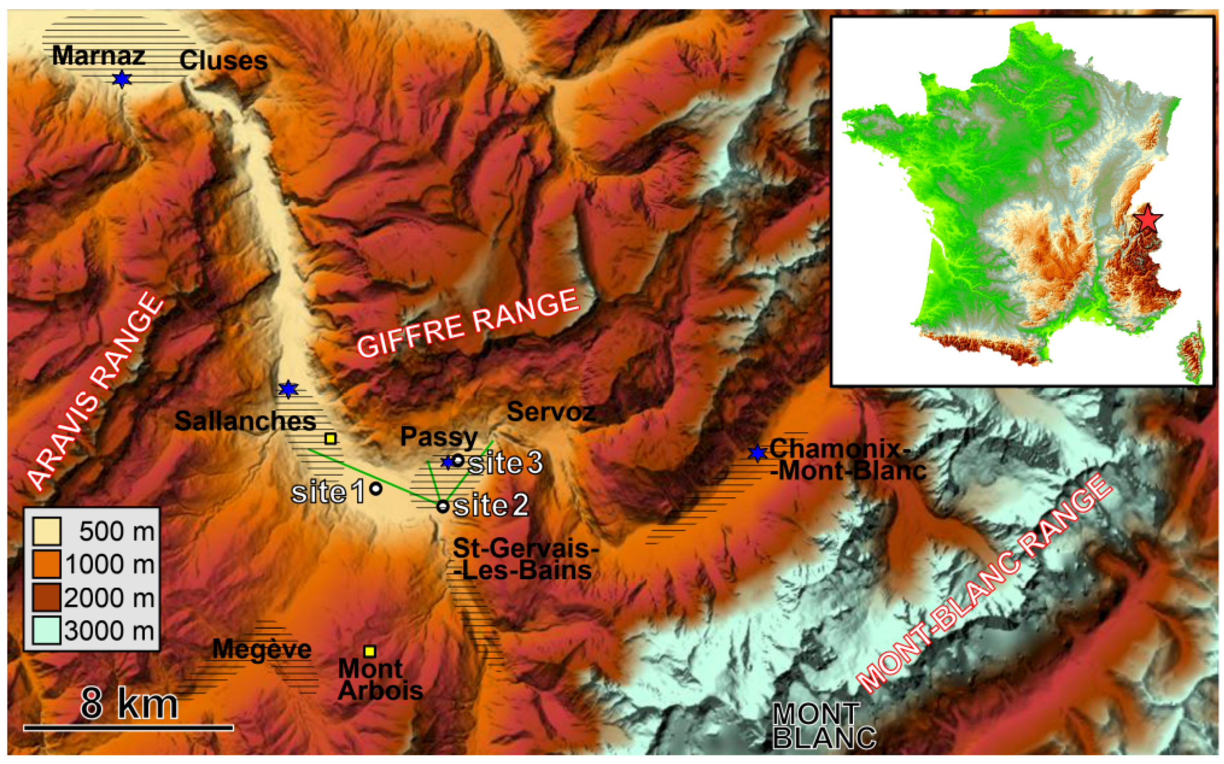
2.1. Context: A Steep Sided Polluted Alpine Valley

The Arve River Valley is located in the French Alps close to the border between France and Switzerland. It starts in the vicinity of Mont-Blanc and extends over about 100 km to Lake Geneva. This study focuses on a section of the Arve River Valley close to the town of Passy, hereafter referred to as the Passy basin. The topography of the Passy basin and its surroundings is presented in Figure 1. This section of the valley is approximately 23 km long, has a maximum width of 2 km and an average valley bottom slope of 1 % . The basin is confined by the Giffre range (about 2000 m Above Sea Level (ASL)) to the north, the Aravis range (about 2000 m ASL) to the west and the Mont-Blanc range (rising to 4808 m ASL) to the southeast. The floor in the centre of the Passy basin is around 560 m ASL, giving a valley depth of more than 1500 m. The Passy basin is connected with the upstream part of the Arve river valley (Chamonix, 1030 m ASL) and the downstream part (Marnaz, 480 m ASL) through two constricted passageways, at Servoz and Cluzes, respectively. At Servoz, the valley is less than 50 m wide and its floor rises by 200 m over a distance of 4 km. This forms a natural barrier between the upper part of the valley and the Passy basin. Two smaller tributary valleys are connected to the south of the basin, orientated in a northeasterly direction (“Megève” valley) and northwesterly direction (“Saint-Gervais” valley).
The Arve river valley regularly experiences severe pollution episodes in winter. The valley is urbanized, with 27,000 residents within the Passy basin (Passy, Sallanches), 10,000 residents in the upstream town of Chamonix and about 6000 residents in each of the southern tributary valleys (Megève and Saint-Gervais). An Atmosphere Protection Plan [31] has been in force for the whole Arve River Valley since February 2012 for winter PM10 pollution episodes among other things. PM10 can have anthropogenic or natural origins, the former being the main source of pollution within the valley. Anthropogenic PM10 results from residential heating (wood burning), transport (the valley has been one of the major access roads to Italy through the Mont-Blanc tunnel since it was opened in 1965) and industrial emissions.
In 2015, the local air quality agency, Atmo Auvergne-Rhône-Alpes, recorded 44 and 20 days when PM10 concentration exceeded the air quality standard at Passy and Sallanches, respectively [33]. In contrast, the neighbouring cities outside the Passy basin were significantly less affected, with 10 days at Chamonix (20 km up the valley) and only 3 days at Marnaz (20 km down the valley). Figure 2a displays the time evolution of PM10 for the four towns through January and February 2015. Grey areas represents the pollution episodes based on PM10 levels measured at Passy. It can be seen that PM10 time series at Passy and Sallanches display similar trends. However, concentrations at Sallanches remain systematically lower during pollution events, whereas the two towns are only 5 km apart. At Chamonix, the PM10 time series appears significantly distinct from those at Passy and Sallanches during pollution peaks but remains similar the rest of the time. Table 1 lists the pollution episodes represented in grey and gives the day of the episode during which the maximum PM10 concentration was reached for the three stations. While the maximum was reached on the same day for the two stations within the Passy basin, it was shifted towards the beginning or the end of the episodes for the Chamonix up-valley station.
Figure 2b displays the time evolution of the sea level pressure (Psea) measured in the middle of the Passy basin. In addition, the Psea time series recorded by the METEO-FRANCE automatic weather station at Annecy, 45 km west of the Passy basin, is represented. The two series are very close, with an average difference of 0.65 hPa and a maximum difference of 3.5 hPa. Annecy Psea measurements can therefore be used to complete data missing from the Passy Psea series. The temperature gradient between 540 and 1833 m ASL is represented in blue. It was computed using METEO-FRANCE automatic weather stations of Sallanches (541 m ASL) and Mont-Arbois (1833 m ASL). It appears that pollution episodes occur during anticyclonic conditions, which favour the development of persistent temperature inversion ( d T / d z > 0 ), as already noted by [34,35,36].
The high levels of PM10 and the spatial variability could be explained by emissions rates and/or local dynamics. However, the emissions cannot solely explain the important pollutant levels, which are similar or higher than the levels measured in more urbanized areas. For instance, the nearby urban area of Lyon, which is the third most densely populated city in France, show lower wintertime PM10 levels while there are 50 times more residents. A better understanding of the local mechanisms within the Passy basin and its vicinity is therefore needed to understand its importance on pollutant dispersion. This was one of the main reasons for the Passy-2015 field experiment.

2.2. Objectives and Overview of the Field Experiment

The Passy-2015 field experiment was designed to give a better understanding of the atmospheric dynamics in the Passy basin under anticyclonic wintertime episodes and improve numerical weather prediction and air quality models in these conditions. More precisely, the objectives were to determine which mechanisms may:
  • lead to the high PM10 concentrations observed in the Passy basin during winter,
  • participate in the spatial variations of PM10 concentrations observed within the Passy basin and its vicinity,
  • pilot the time evolution of PM10 concentrations (diurnal cycle and over the whole episode).
The field experiment was conducted in winter 2014/2015, from November 2014 to April 2015, with a larger set of instruments in January and February 2015 [29]. Observations were reinforced during two Intensive Observation Periods (IOPs) in February 2015. IOPs were planned according to weather and air quality forecasts. The first one took place from 6 to 14 February and the second from 17 to 20 February, corresponding respectively to episodes 3 and 4 of Table 1. The present study focuses on IOP1, which was the most thermally stable and polluted of the two IOPs as shown in Figure 2. A persistent temperature inversion developed from 9 to 13 February. Largeron and Staquet [9] have suggested that the use of a simple temperature gradient can be relevant to describe the overall thermal inversion dynamics and the PM10 concentration evolution during a pollution peak. Based on this consideration and on Largeron et al. [37], the three phases of the persistent inversion cycle during IOP1 are defined as:
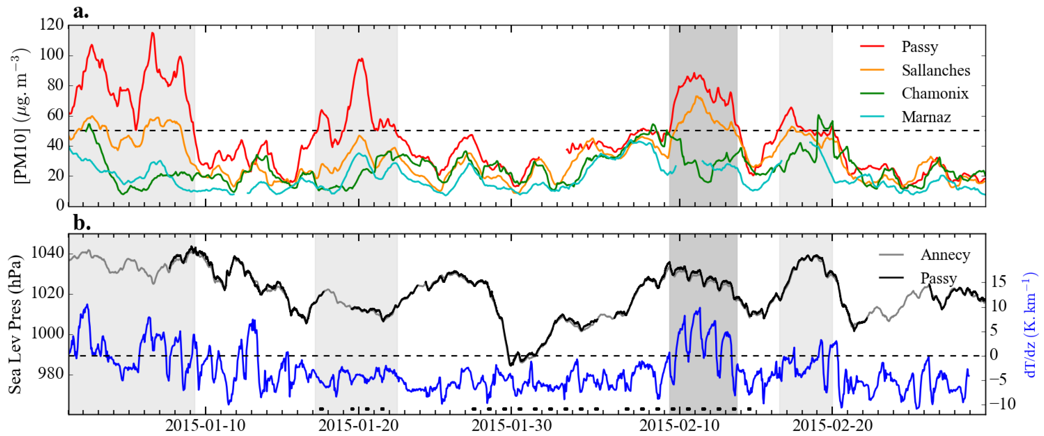
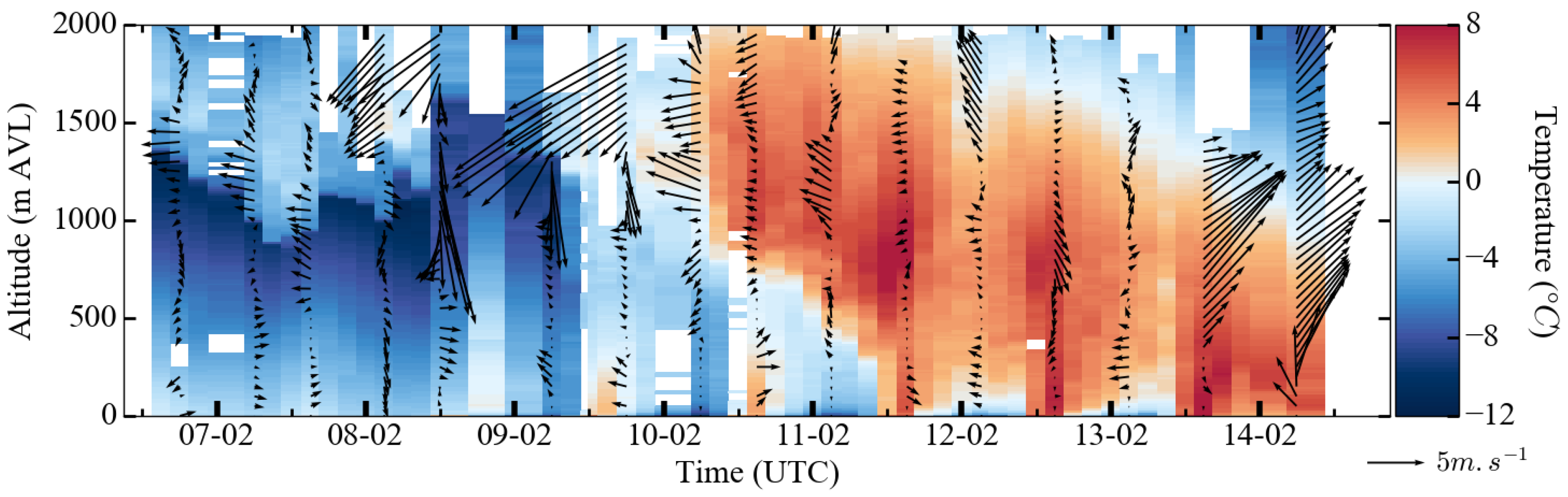
  • the formation stage: an anticyclone formed at the beginning of IOP1 and reached a pressure maximum on the morning of 9 February. The temperature inversion became established during the same day, with a reduction of the synoptic wind and an advection of warm air above the Passy basin (Figure 3). This advection generated a capping inversion, which favoured the decoupling of the atmosphere within the valley from the atmosphere above and thus allowed the development of local dynamics. This stage was associated with an increase of the temperature gradient as observed in Figure 2.
  • the stagnation stage: from 10 to 12 February, the capping inversion persisted over the period with its top lowering slowly day by day. A ground-based inversion developed at night and was destroyed in the early afternoon because of weak convection. The maximum intensity of the temperature inversion was reached on 11 February at 6:00 a.m. UTC.
  • the destruction stage: the sea level pressure dropped during the night of 13 February and the temperature gradient became negative. This was explained by the elevated inversion erosion caused by an increasing synoptic wind and a rain episode on 14 February. Figure 2 shows that this rain event appeared coincidently with the drop in the PM10 concentrations.
In this study, we focus our analysis on the wind dynamics within the Passy basin in the first few hundred metres above the ground. The main objective is to characterize the wind dynamics during this persistent temperature inversion episode, and to identify which features may contribute to the observed PM10 concentration heterogeneities described previously.

2.3. Instrumentation and Measurement Strategy

Figure 1 and Table 2 present the instruments used in this study and the three corresponding sites deployed within the Passy basin. A complete description of the large set of instruments deployed is available in [29]. Situated in the valley centre, Site 1 was the most instrumented. Its elevation is taken as the valley level reference and used to define elevation in metres Above Valley Level (m AVL). Site 1 was dedicated to the vertical description of the atmosphere from the ground up to a few kilometres AVL. A profiler Doppler wind lidar (DWL) the WLS8-5 was used in this study. It provided profiles of wind speed and direction every 3 s from 40 m up to 500 m AVL with a 20 m vertical resolution. More technical details of the WLS8-5 specifications are given in Table 3. During IOPs, radiosoundings were launched every 3 h using a technique of reusable radiosondes developed by Legain et al. [38]. Radiosoundings provided profiles of wind, temperature and humidity, with a 10 m vertical resolution up to 2000 m AVL. Fog episodes were detected using data from a Present Weather Detector (PWD22) and a Ceilometer (CT25K). The CNR1 net radiometer measuring radiative fluxes was used to derived the surface albedo. The bare ground has an albedo of 0.2 and a threshold of 0.5 was used to identify the days with snow cover (black dots in Figure 2).
Site 2 was installed in the southeastern part of the valley, 2.6 km away from Site 1 and about 40 m higher. The main purpose of this site was to describe the spatial variability of the lower levels of the atmosphere. Its panoramic view permitted scanning of the atmosphere with horizontal and vertical cross-sections. A scanning DWL was deployed and will be described in the following section. The pollutant monitoring was performed at Site 3 by an automatic TEOM-FDMS station of the local air quality agency Atmo Auvergne-Rhône-Alpes. It provided hourly-averaged PM10 concentrations. TEOM-FDMS stations are also routinely-operated at Sallanches, Marnaz and Chamonix (blue stars in Figure 1). Finally, some of the 20 Meteo-France automatic weather stations located in the area of interest were also used in this study (Annecy, Sallanches and Mont-Arbois, yellow squares in Figure 1).

3. Material: WLS200S Lidar

The database analysed here was provided mainly by a 3D long range DWL, the WLS200S, developed by Leosphere [39] and located at Site 2. Another DWL, the WLS8-5 located at Site 1 is also used.

3.1. Lidar Specifications

3.1.1. Instrument Description

The WLS200S and WLS8-5 specifications are given in Table 3.
A DWL is an active remote sensing instrument that emits a laser pulse into the atmosphere and records the radiation backscattered by particles. The WLS200S operates at a wavelength of λ = 1.54 μ m , which means that the laser beam is mainly scattered by atmospheric aerosol particles having diameters above about 100 nm. Because of their movements relative to the instrument, the backscattered signal is subject to the Doppler effect and its frequency is shifted compared to the emitted laser pulse frequency [40]. Since the particle movements are assumed to follow the wind, the frequency shift is proportional to the wind velocity in the Line-Of-Sight (LOS) direction. This leads to the relation Δ f = 2 V l o s c , where c corresponds to the speed of light and V l o s to the LOS velocity, counted positive when the wind is blowing away from the lidar.

3.1.2. Measured Quantities

The WLS200S provides high resolution range-resolved measurements of:
  • the Line-Of-Sight velocity ( V l o s ) in m·s 1 . Negative velocities represent a flow toward the lidar while positive velocities indicate a flow away from the lidar. To facilitate the plot interpretation, a convention based on the north–south or west–east direction is applied in this study whenever possible, and is specified in the figure caption.
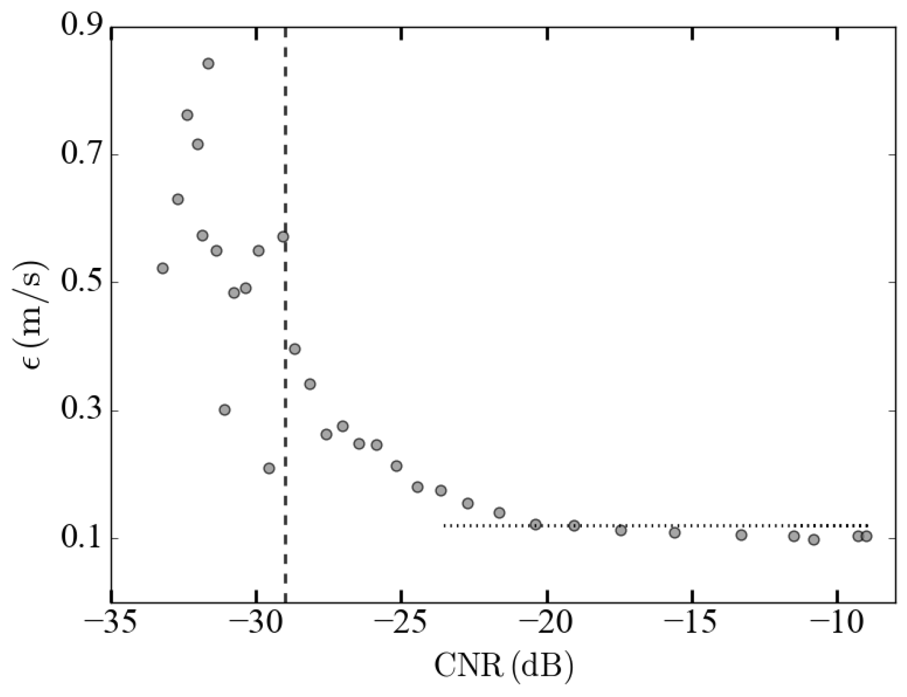
  • the Carrier to Noise ratio (CNR) in dB, corresponding to the ratio of the power of the received heterodyne signal to the noise power. The CNR depends, among others things, on aerosol content and can be expressed by the Equation (1) [41]:
    C N R ( R ) = 10 l o g 10 1 R 2 I ( R ) β ( R ) T 2 ( R ) ,
    where R represents the distance from the lidar in the LOS direction, β ( R ) is the backscatter coefficient, T 2 ( R ) = e x p ( 2 α R ) is the atmospheric transmission (with α being the extinction coefficient) and I ( R ) gathers together the geometric dependences on R, including the heterodyne efficiency, which mainly affects the signal in the nearest range gates. The CNR gives an indication of the measurement quality and is used for data quality checking (Appendix A).

3.1.3. Limitations

Under clear sky conditions, the lidar sensitivity depends on the aerosol content meaning that pollution episodes are favourable to longer ranges. Under fog conditions, high extinction caused by water droplets may lead to a severely reduced range. Long distance ranges are automatically discarded by the CNR thresholding during fog episodes. These episodes detected by PWD22 and CT25K are consistent with the time periods filtered by the CNR thresholding. The most important episodes occurred in the nights of 10 to 11 and 11 to 12 February.

3.2. Scanning Strategy

During the Passy-2015 field experiment, the WLS200S was operated with the following strategy:
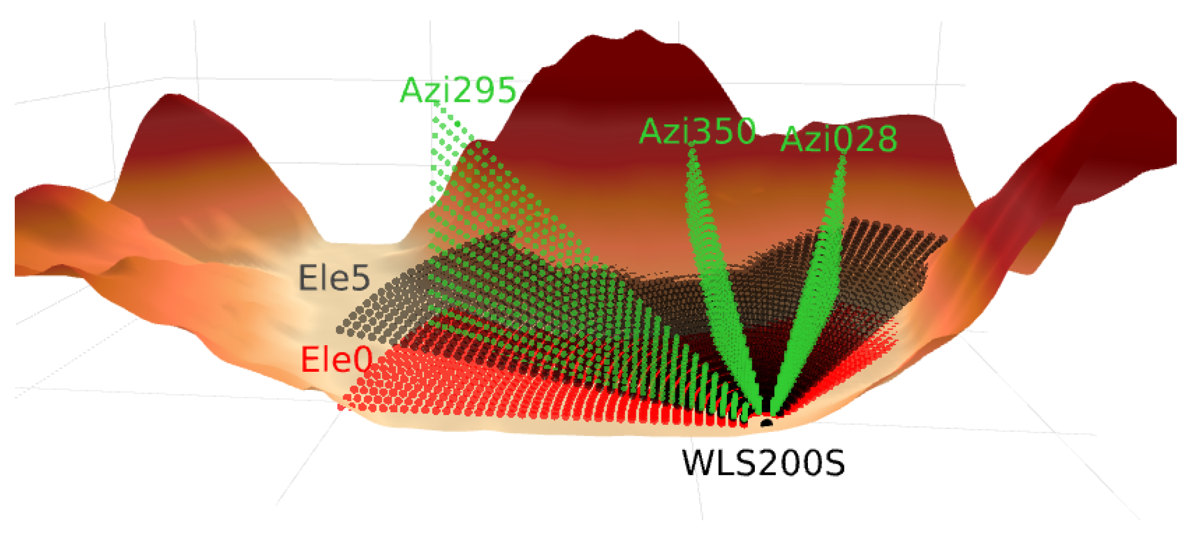
  • An horizontal Plan Position Indicator scan (PPI) every 10 min. This was obtained by the lidar beam scanning in azimuth, between 250° and 60° with respect to the north, while keeping the elevation angle at 0° (in red in Figure 4). Horizontal PPIs allowed the structure of the horizontal valley wind, 40 m AVL, to be investigated.
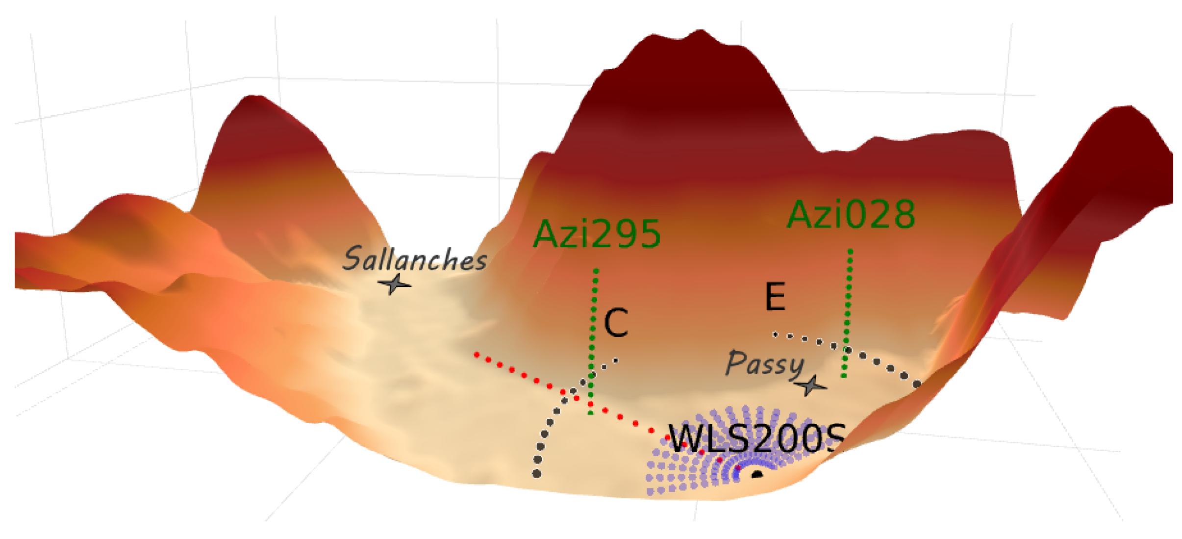
  • A set of three Vertical Range Height Indicator scans (RHI) every 30 min, obtained by maintaining a constant azimuth angle of the lidar beam and scanning vertically between 0° and 90° in elevation (in green in Figure 4). RHI scans were performed in three azimuth directions: 295°, 350°, 28° in order to capture the vertical structure of the wind in the along-valley direction (azimuth 295°), along the north slopes (azimuth 350°) and in the eastern part of the basin close to the Servoz passageway that leads to the upstream part of the valley (Chamonix). The baselines of RHI scans are indicated by the green lines in Figure 1.
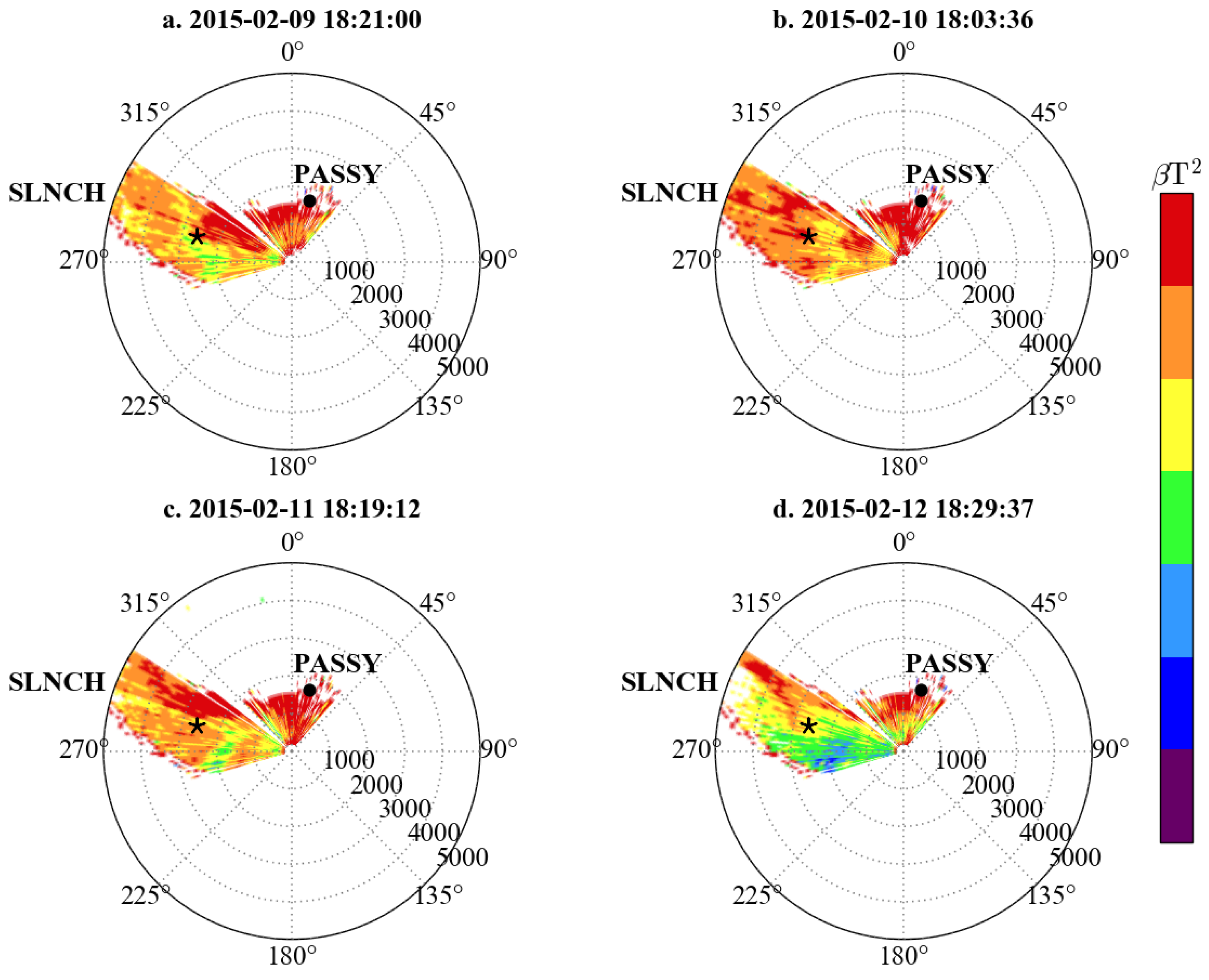
  • Meanwhile, a set of slanted PPI scans was obtained every hour by scanning the lidar beam in azimuth between 250° and 60° and gradually increasing the elevation angle between 1° and 15°. An example of PPI scan at elevation 5° is represented in black in Figure 4.
This strategy provided a three-dimensional volume of measurement within the valley every hour, with a resolution of 100 m. The system was set with 59 ranges gates, of size 100 m, giving a potential maximum range of 6 km.

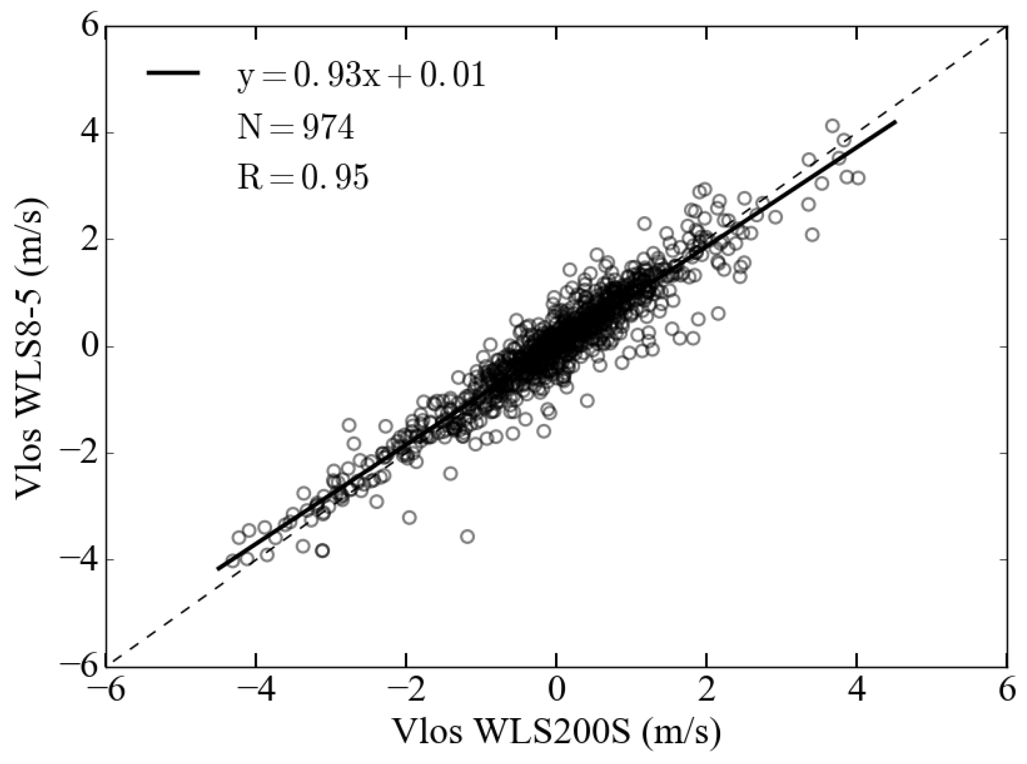
3.3. Inter-Comparison

In this section, V l o s , measured from the WLS200S, and the same quantity derived from zonal and meridional velocities measured by the WLS8-5, are compared. DWL profilers have been used increasingly for atmospheric and wind turbine studies in the last decade. Comparison studies have shown very good agreement with readings from mast-mounted anemometers, with a correlation coefficient R 2 = 0.99 [42], or with radiosonde wind measurements [43]. The WLS8-5 is thus considered as a reference in the current study.
The comparison was made using the first gate of the WLS8-5, 40 m AVL at Site 1, and the closest WLS200S measurement extracted at azimuth 287°, 2600 m in the LOS direction. One-minute-averaged zonal and meridional velocities from the WLS8-5 were computed and the corresponding LOS velocity was derived by applying Relation (2):
V l o s = u s i n ( γ ) v c o s ( γ ) ,
where u and v represent zonal and meridional components, respectively, measured by the WLS8-5 and γ the azimuth angle of the WLS200S. The result of the comparison is displayed in Figure 5 and reveals a very good correlation between the two lidars with a correlation coefficient of R = 0.95 . The linear regression slope ( s = 0.93 ) indicates that the V l o s derived from the WLS8-5 are slightly under-estimated in comparison to those measured by the WLS200S. An explanation for this under-estimation may be the difference in observation volumes of the two instruments. The WLS200S performs an integration over a very thin horizontal cylinder 100 m long, whereas the WLS8-5 performs an integration over a 3D cone of approximately 21 m mean diameter and 20 m height.
To evaluate the consequence of these differences in the volume of integration, the same comparison was made by considering only the cases in the time range 10:00 a.m.–4:59 p.m. UTC that were likely to be more homogeneous along the vertical because of convective mixing over the first 500 m (see Figure 3). This subset gave a similar correlation coefficient and a linear regression slope much closer to 1 ( s = 0.98 ), suggesting that the more homogeneous the wind is in the vertical direction, the better is the comparison. This suggests that at least a part of the slight underestimation of the WLS8-5 measurements relative to the WLS200S ones was due to the differences of the volume of integration in the vertical direction.
This comparison finally allows a validation of the WLS200S database. This was confirmed by a determination of the error on V l o s measurements, which showed that 80 % of the database has a mean error of 0.12 m·s 1 (Appendix A) .

4. Results

This section is divided into three parts: Section 4.1: a general overview of the wind intensities over a winter, Section 4.2 the characterization of the along-valley wind during the IOP1 with spatial and temporal analysis and Section 4.3 the identification of flows coming from the Saint-Gervais and Megève tributary valleys.

4.1. Overview of the Wind Intensity over a Winter

This section aims to provide a general overview of the wind distribution under stable conditions compared with more vertically mixed conditions. Figure 6 represents box plots of V l o s extracted at 40 m AVL at two locations within the basin. These locations were chosen so that characteristics of the along- and cross-valley wind components could be inferred. Along (cross) valley components were extracted at azimuth 287° (350°) and 2600 m (700 m) from the lidar. Blue boxes represent the January–February database (Jan–Feb), which contains a large range of wintertime atmospheric conditions and associated wind patterns. Red boxes correspond to the stagnation stage of IOP1, described in Section 2.2 (10–12 Feb). The bottom and top of the box correspond to the 25th and 75th percentiles and the whiskers extend from the 1st to the 99th percentile, meaning that 98 % of the database is between the two whiskers.
For both along- and cross-valley winds, the extrema are significantly reduced for the 10–12 Feb dataset. This means that stable conditions limit the ventilation. To evaluate the distribution symmetry, the skewness ( γ 1 ) was computed. For along-valley winds, the Jan–Feb distribution is symmetric, whereas the 10–12 Feb is negatively skewed with γ 1 = 0.27 . This asymmetry means that, over the period, there was a range of wind intensity, above 1.2 m·s 1 , for up-valley winds that was not observed for down-valley winds. For cross-valley winds, the distribution ranges are less spread than for the along-valley component, which is consistent with the steep-sided basin shape. Both distributions are positively skewed meaning that, at least at the location considered (north of Site 2), the cross-valley winds blow more frequently from the south.
Finally, this figure shows that the wind intensities are significantly weaker in the Passy basin bottom during stable conditions than in the full two months database. The observed asymmetry on both the cross and along valley wind distributions may be of major importance for pollutant dispersion. In the following, the analysis focuses on the dynamics during the persistent temperature inversion episode.

4.2. Spatio-Temporal Fluctuations of the Along-Valley Wind

The along-valley wind is analysed in the three directions represented in Figure 7:
  • along two vertical profiles (green lines) extracted in the centre (Azimuth 295°) and eastern part of the basin (Azimuth 28°), 2000 m away from the lidar, with data available every 30 min.
  • along the horizontal valley axis (red line), 40 m AVL, with data available every 10 min.
  • across the valley, along cross-valley transects (black lines) in the centre and eastern part of the Passy basin, with data available every 1 h.

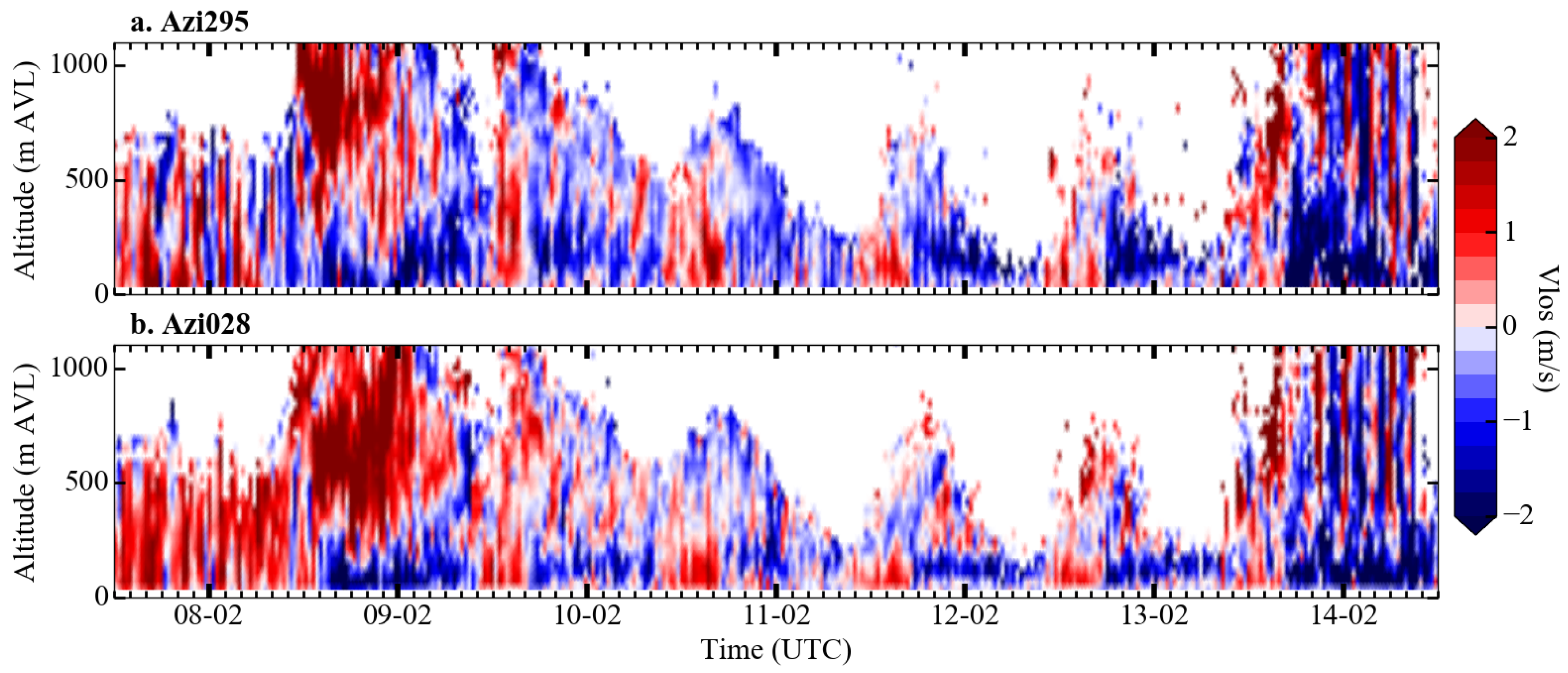
4.2.1. Vertical Structure

Figure 8 presents space and time (z,t) diagrams of V l o s , extracted for two vertical profiles within the Passy basin (green lines in Figure 7). Each panel represents the time evolution of the profile, extracted at azimuth 295° in the centre of the basin (panel a) and at azimuth 28° in the eastern part of the basin (panel b). Red corresponds to up-valley winds (approximately westerly in the basin centre) and blue to down-valley winds (approximately easterly).

Vertical Range

The vertical range of the WLS200S (hereafter denoted H W L S ) changes over the period. From 7 to the middle of 8 February, H W L S remains approximately constant at around 700 m AVL. This height is consistent with the cloud base detected by a ceilometer at Site 1. The clouds dissipate at noon UTC on 8 February, the time at which H W L S increases. Then, a diurnal cycle starts, which lasts until 13 February (i.e., during the stagnation stage of the temperature inversion episode). H W L S starts its increase around 10:00 a.m. UTC, when convection begins in the low-level layers, and reaches its maximum between 4:00 p.m. and 6:00 p.m. UTC everyday. Then, it decreases during the night and reaches its minimum around 8:00 a.m. UTC the next day. The day-to-day comparison shows that H W L S tends to decrease slightly during the episode, probably following the aerosol layer thickness. Its daily-maximum ranges from 1400 m AVL on 9 February at 4:00 p.m. UTC to 650 m AVL on 12 February. This reduction is first driven by an increasing stability at the beginning of the episode, which confines the pollutant within a thinner layer. Afterwards, it may result from the subsidence of the capping inversion (Figure 3). Finally, H W L S behaves in a very similar way over the two profiles, which highlights the homogeneity of the aerosol layer structure within the Passy basin. Note that H W L S may be perturbed by fog episodes in the early morning and is therefore more difficult to interpret.

Wind Dynamics

Figure 8a shows the onset of the up-valley wind in the valley centre, which occurs around 10:00 a.m. UTC and coincides with the vertical range increase. The mean up-valley wind intensity and depth tend to decrease during the stagnation stage. The layer develops up to 500 m AVL on 9 and 10 February, then decreases to a depth of around 200–300 m AVL on 11 and 12 February.
The down-valley wind starts at 5:00 p.m. UTC and is characterised by a jet-like structure that varies in thickness, elevation, and intensity over the period:
  • The signature of the jet is pronounced during the night of 9 to 10 February with wind oscillations. The first hundred metres above the ground are the most affected by oscillations, with hourly wind reversal (more details in Section 4.2.2).
  • The down-valley wind intensity is very weak on the night of 10 to 11 February This induces poor ventilation in the Passy basin boundary-layer, which is mainly affected by wind oscillations and waves.
  • During the following night from 11 to 12 February, the jet forms at around 200 m AVL and then descends, reaching 120 m AVL in the early morning. Its upper structure is out of reach, probably because of signal extinction.
  • For the last night of the episode, from 12 to 13 February, the jet forms at lower altitude (40 m AVL) with a base slightly disconnected from the ground, resulting in an almost motionless surface layer.
The recurrence of the alternation between up-valley winds during the day and down-valley winds at night throughout the episode shows that the circulation is thermally driven, as expected under winter conditions [10]. The morning transition (from down- to up-valley wind) occurs 1 h 40 min after the local sunrise, which is at around 8:20 a.m. UTC according to the Site 1 observations. The evening transition is close to the local sunset, which occurs at 3:50 p.m. UTC. Those delays are consistent with those observed in the Cadarache valley by Duine et al. [27]. It is interesting to note that the daytime and nightime maximum wind intensities are similar. In comparison, up-valley winds three times stronger than down-valley winds have been reported by Giovannini et al. [22], who focused on late spring and summer periods in the Adige Italian valley. However, it is important to bear in mind that, during the wintertime period considered in the present study, the energy available from solar insolation to support the up-valley wind is significantly lower.
In the eastern part of the basin, the morning and evening transitions occur at the same times, but Figure 8b shows a more strongly layered structure. The down-valley wind layer remains at constant elevation (130 m AVL) and has a mean thickness of 80 m. Above this layer, an up-valley wind is observed intermittently during the night. Differences between the two parts of the basin will be discussed in greater details in Section 5.1.

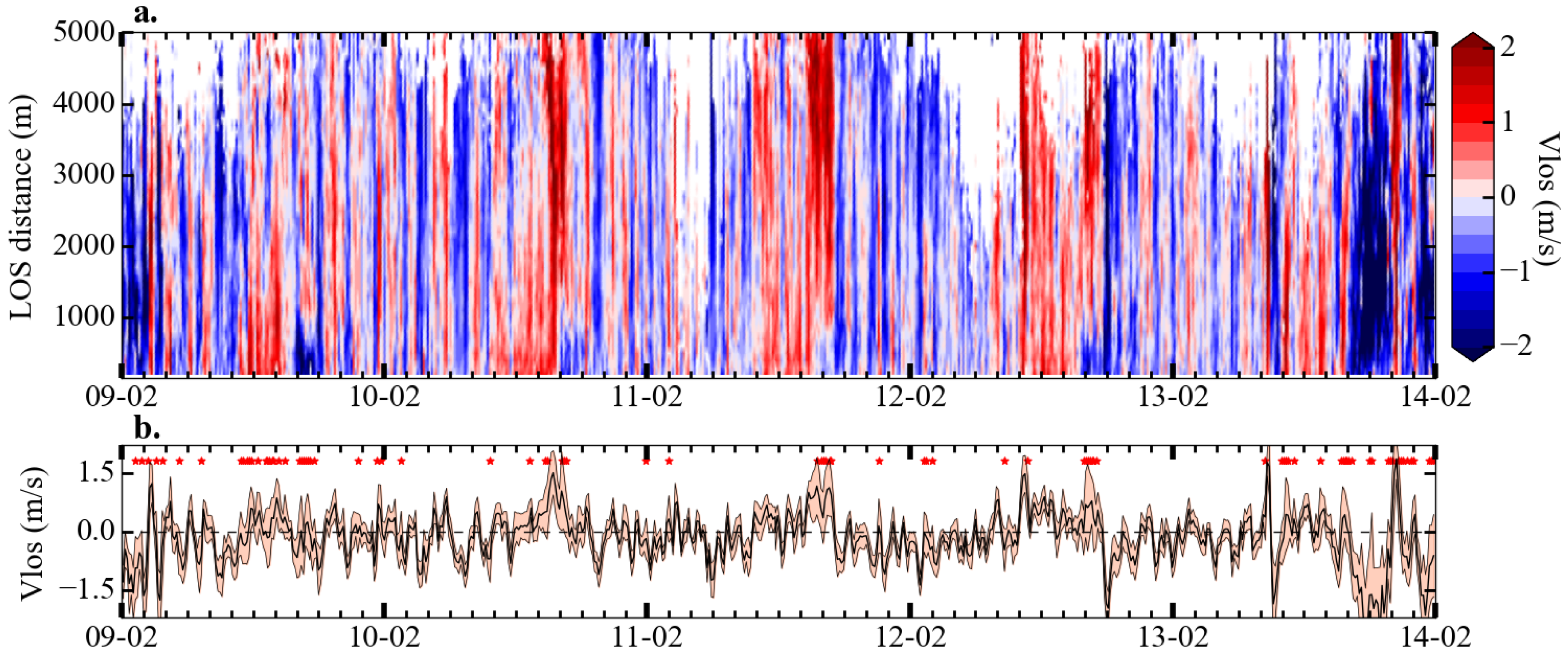
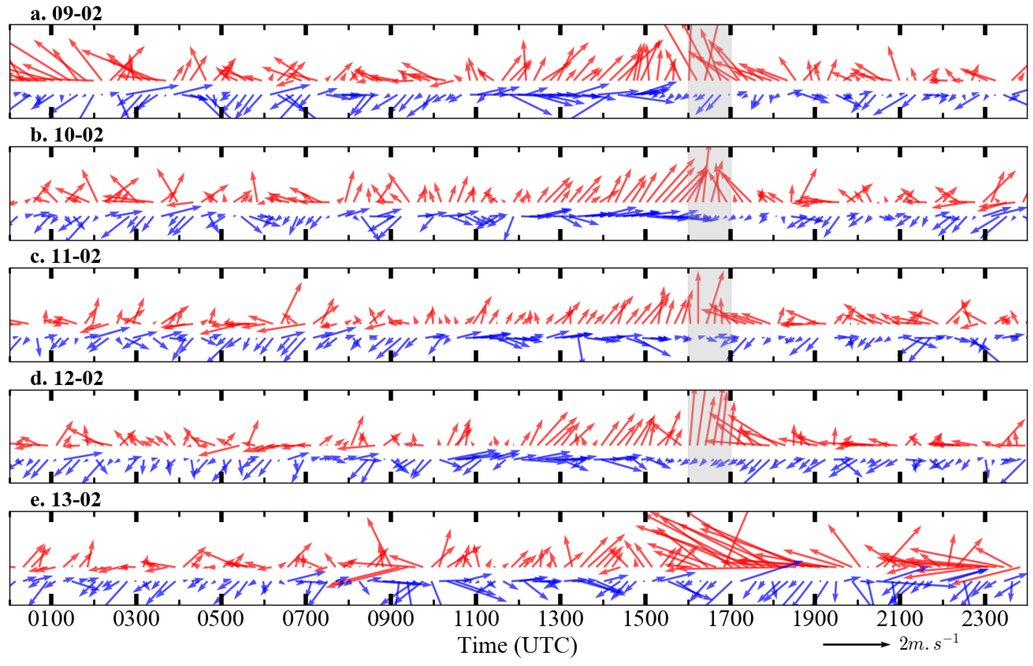
4.2.2. Horizontal Structure along the Valley Axis

The wind structure along the valley axis is investigated here by looking at the V l o s field along the red axis marked in Figure 7. Figure 9a shows a space and time (x,t) diagram of V l o s with the axis of ordinates representing the horizontal LOS distance from the lidar, located at the origin. The colour convention is the same as in Figure 8.
Unlike the vertical range of the lidar, the horizontal range does not follow a diurnal variation. Because the lidar laser beam remains in the aerosol layer close to the ground, the horizontal range remains constant at around 5 km, except in the early morning periods probably because of fog episodes.
The morning and evening transitions of the along-valley flows at 40 m AVL are consistent with those presented in the previous section. Oscillations can be observed in the wind pattern behaviour, especially during the night-time. These oscillations may explain the asymmetric distribution observed in Figure 6, which shows a slight predominance of up-valley winds during the stagnation stage of the temperature inversion (from 10 to 12 February). Up-valley winds are more continuous than down-valley winds that are largely affected by oscillations and do not achieve a stationary state. The 10 min time resolution allows a visual estimation of the wind reversal period close to 1 h . A Fast Fourier Transform was applied to quantify these oscillations more accurately, but the resulting power spectrum did not permit a clear period determination (not shown). We suspect that this may have been the result of an over-complex signal, including oscillations caused by several mechanisms such as the emission of internal gravity waves in the valley by the intrusion of katabatic winds [44] or flow from tributary valleys [45], or the along-slope oscillations of katabatic winds [46].
A remarkable feature is that flow reversal often occurs simultaneously over the whole valley, at least along the red line of Figure 7. To quantify the horizontal homogeneity of V l o s along this line, a criterion is applied for each time step. It is classified as non-homogeneous when its standard deviation is above the threshold of 0.5 m·s 1 , and a least 10 % of the LOS dataset is of the opposite sign (to account for the change in direction).
Means and standard deviations of V l o s are displayed in Figure 9b, where heterogeneous cases are identified with red stars. It can be seen that most of the heterogeneities occur during the daytime and more precisely in the late afternoon, during the evening transition. A recurrent heterogeneity is the one occurring systematically at 4:00 p.m. UTC. At that time, the wind first reverses close to the lidar (i.e., from 0 to 1000 m LOS). Then, after 1.5 to 2 h the wind reversal spreads over the whole valley. This 4:00 p.m. UTC wind reversal may be explained by considering the lidar position, which is close to both the southern sidewalls of the Passy basin and to the St-Gervais tributary valley mouth. The former favours the impact of down-slope winds and theory states that these winds usually reverse before valley winds that have more inertia [10,47]. The tributary valley mouth favours the impact of down-valley wind of the St-Gervais valley, which is in the shadow before the Passy Basin (more detail in Section 4.3.1).

4.2.3. Cross-Valley Structure

This section investigates the structure of the along-valley wind over transects perpendicular to the valley axis, at two different locations, represented by the black lines in Figure 7. Slanted PPI scans were used with elevation angles ranging from 1 to 8°. For each elevation angle, a cross-valley transect was extracted 2000 m away from the lidar, providing horizontal transects from 40 m up to 280 m AVL every 35 m. By means of elevation-by-elevation comparisons, three elevations (75, 150 and 250 m AVL) were selected for analysis and are presented in Figure 10. The axis of ordinates represents the cross-valley distance, centred over the horizontal transect considered. Because of the lower scan acquisition frequency (1 scan per hour), data were smoothed with a Gaussian filter to account for the coarse temporal resolution. In contrast to the previous section, where the wind was blowing along the transect considered, we now look at the along-valley wind blowing through the transect over the valley width.

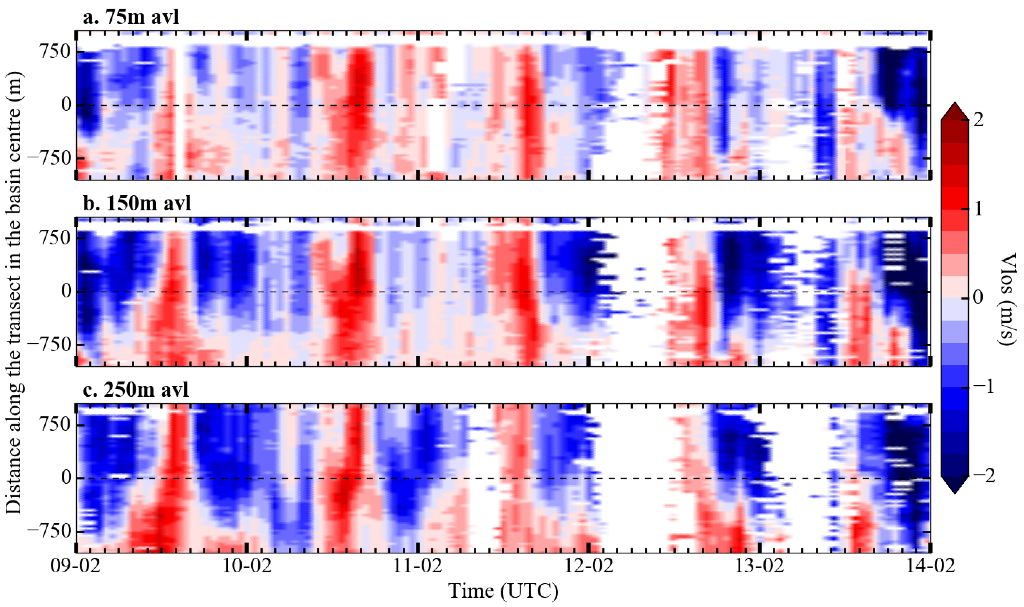
Vertical and North–South Structure for Cross-Valley Transects in the Basin Centre

A comparison of the diagrams obtained from 40 m to 280 m AVL confirms the low wind intensities up to 110 m AVL, with V l o s intensities below 1.25 m·s 1 on the 75 m elevation diagram in Figure 10a, and the more intense systems aloft. At 150 m AVL, the intensities increase during both day- and night-time. The down-valley wind intensity tends to decrease above 250 m AVL (not shown) and the elevation of its core (jet-like structure) changes during the period, as observed in Figure 8. The new and important feature accessible with the visualization is the north–south wind structure. It can be noted that during the day, the up-valley wind develops over the whole valley width. At night, the down-valley flow does not extend over the valley width but is rather confined to the northern half of the basin. The southern half of the basin is affected by a wind blowing in the opposite up-valley direction.

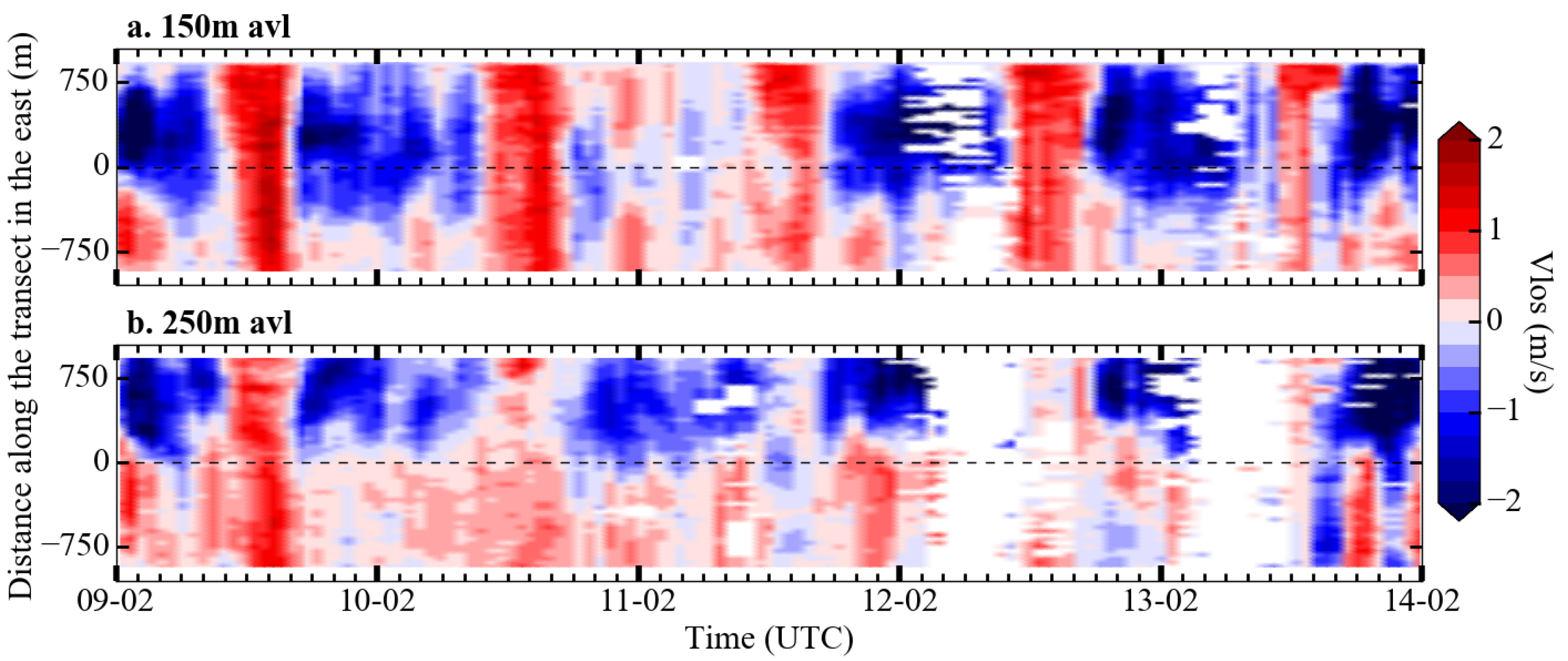
Vertical and North-South Structure for the Eastern Cross-Valley Transects

The same analysis is presented in Figure 11 for cross-valley transects extracted in the eastern part of the Passy basin at elevation 150 m and 250 m AVL, panels a and b, respectively. A similar spatial structure along the y-axis and over the vertical is observed. At night, the down-valley jet is shifted northward as the altitude increases. This may be linked to the widening of the valley with elevation. When the diagrams shown in Figure 10 and Figure 11 are compared, the down-valley jet appears more intense and narrower in Figure 11. For instance, on 12 February at 8:00 p.m. UTC, 150 m AVL, a broadening of the flow towards the west can be observed with a mean velocity varying from 2.8 to the east to −2.1 m·s 1 to the basin centre. The sheared structure is more pronounced in this part of the basin, especially at 250 m AVL, where half of the basin width is affected by wind blowing up-valley at night.
This night-time cross-valley sheared wind structures and its reinforcement in the eastern part of the valley is likely to have very important consequences for pollutant dispersion and will be discussed in more details in Section 5.2.

4.3. Tributary Valley Flows

In addition to the ventilation caused by the along-valley wind system, the basin is also fed by air from outside the valley. This may lead to a dilution or an increase of pollutants within the basin. Two important sources of such air are the Saint-Gervais and Megève tributary valleys (Figure 1).

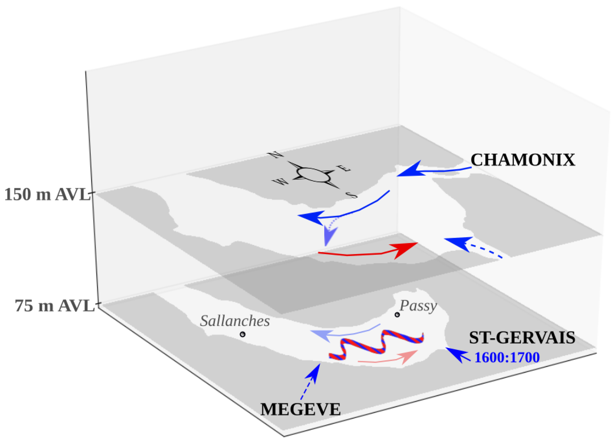
4.3.1. Saint-Gervais Valley

Since the WLS200S was located at the Saint-Gervais valley exit, the flow penetrating into the basin could be detected using horizontal PPI scans. At low elevation (40 m AVL), a wind intrusion coming from the south is observed at around 5:00 p.m. UTC on WLS200S horizontal and vertical scans (not shown). This intrusion penetrates into the valley over a restricted area (on average 1000–1500 m from the WLS200S in the LOS direction) and then vanishes. Figure 12 synthesizes this information by showing the direction of the prevailing flow blowing through a restricted zone close to the WLS200S. This zone is defined between two circular arcs, one of radius 200 m and the other 1000 m, in the sector from azimuth 250° to 60° (blue area in Figure 7). For each azimuth of the horizontal PPI scan, a spatial average of V l o s ( V l o s ) is computed. The azimuth of the maximum V l o s is considered as the direction of the dominant away-from-lidar wind component blowing through the arc. Conversely, the azimuth of the minimum V l o s represents the direction of the dominant toward-lidar wind component. Red (blue) arrows represent the away-from-lidar (toward-lidar) wind components in terms of direction and mean intensity. It should be noted that these components may be the result of a flow superimposition.
From Figure 12, it can be seen that the low-level southern intrusion is observed between 4:00 p.m. and 5:00 p.m. UTC, with the dominant red away-from-lidar component blowing from the south, every day from 9 to 12 February (grey areas on panels a to d). This direction is consistent with the relative orientation of the Saint-Gervais valley compared to the WLS200S location. Vertical scans show that the thickness of this wind layer does not exceed 100 m meaning that it affects only the lowest level of the basin atmosphere (not shown). The only day during which the intrusion signature is not observed is the 13 February, but it may have been masked by the down-valley wind, which was more intense during the destruction stage of the temperature inversion episode (Figure 8 and Figure 9).
Looking at the diurnal evolution, before 4:00 p.m. UTC, it can be seen that the domain is mainly affected by the up-valley wind with directions of the away-from- and toward-lidar components consistent with the valley axis direction. From 5:00 p.m. UTC, the circulation reverses to down-valley wind. The early morning presents a similar pattern, but the winds are more fluctuating.
Wind intrusions were also visible on vertical lidar scans at higher elevation, in the range 200–540 m AVL (not shown). These flows may also affect the basin dynamics by interacting with the down-valley flow presented in Section 4.2.

4.3.2. Megève Valley

Due to the relative orientation of the Megève tributary valley with respect to the WLS200S location, the flow that may exit this valley is mainly perpendicular to the lidar beam and cannot be seen on V l o s measurements. However, information can be captured using a method based on the CNR signal, which depends among other things on aerosol content (Section 3.1.2). Based on Fujii and Fukuchi [40] and Chouza et al. [41], a correction was derived to remove instrumental dependence of the CNR (Equation (1)). This gives access to the attenuated backscatter ( β T 2 ) defined by:
β T 2 = l o g 10 10 0.1 C N R ( R ) R 2 I ( R ) .
The instrumental function I(R) was determined in the same way as in Chouza et al. [41], i.e., by fitting the heterodyne efficiency function given by their Equation (12) on cases considered as homogeneous with regard to aerosol distribution. Additional signal processing steps would be needed for PM10 retrieval, but this correction is sufficient for a qualitative analysis of the attenuated backscattered intensity within the basin.
Horizontal maps of β T 2 derived from horizontal PPI scans measured around 6:15 p.m. UTC from 9 to 12 February are displayed in Figure 13. β T 2 increases as the colour moves towards the red. Looking at the western part, in the azimuth range 250 to 310°, a yellow structure crossing the valley can be observed. This structure probably represents an advection of air by the flow coming out of the Megève tributary valley, which connects with the Passy basin at this location. The color of the structure suggests an air mass that is cleaner than the air within the basin. It is visible from 4:30 p.m. UTC for the four days and was also intermittently present during the whole night (not shown). The similarity between this onset time and that of the Saint-Gervais valley exit flow observed in Figure 12 suggests a similar dynamics between the two tributaries, which share a similar north–south orientation.
A noteworthy feature was a meandering of the flow, with significant direction changes observed over a 10 min period (not shown). These meanders are often observed under stable conditions and low wind intensities [48]. They may influence pollutant dispersion and may also be one of the sources of the oscillations observed in Figure 9.
Close to the northern sidewalls and in the eastern part of the basin, red patches are observed that are likely to be associated with more polluted air in these areas than in the southern part of the basin.
The day-to-day comparison shows a generally lower signal on 12 February (Figure 13d) that is consistent with the PM10 diminution observed within the Passy basin in Figure 2.
Finally, this method constitutes a complementary approach to the V l o s analysis by providing information on a flow perpendicular to the LOS. Moreover, it provides qualitative information on the aerosol content of the air. Its unique ability to retrieve information on the 3D wind structure makes it a very important instrument for studying wind dynamics over complex terrain.

5. Discussion

5.1. Cause of the Observed Wind Patterns

The daytime up-valley wind develops homogeneously within the basin, whereas the night-time wind system is more complex. Figure 14 presents a conceptual scheme of the main wind structures observed at night during the stagnation stage of the persistent inversion with:
  • a low-level layer below 100 m AVL mainly driven by oscillations reflecting the cold air pool perturbations and limiting the ventilation of the low-level layer in the basin,
  • a down-valley jet-like structure around 150 m AVL on the northern side, stronger and narrower in the eastern part of the Passy basin,
  • a shear zone in the north–south direction with a down-valley flow running along the northern sidewalls and a wind blowing in the opposite up-valley direction in the southern half of the basin. This pattern is more pronounced at 150 m AVL.
  • the flows drained by the two tributary valleys, Megève and Saint Gervais, which are observed intermittently during the night.

5.1.1. Down-Valley Jet within the Passy Basin

The down-valley jet observed within the Passy basin may arise from several contributions coming from the surrounding valleys. First, because of the jet elevation 130 m AVL observed in Figure 8b, the down-valley wind observed in the east is likely to come from the upstream Chamonix valley. The Servoz passageway between the Chamonix valley and Passy basin is a very narrow (50–200 m) meander with an elevation of around 150 m AVL at the basin entrance, consistent with the 130 m AVL elevation of the jet. This “main” flow is then mixed with the down-valley flows coming from the two tributary valleys in the south sidewalls of the Passy basin, Saint-Gervais and Megève, as observed in Figure 12 and Figure 13, respectively. The time lapse of 1 h between the apparition of the tributary down-valley flows and the main down-valley flow may be the result of the side valleys being in shade earlier because of their north–south orientation. Their mixing in the middle of the valley may change the relative buoyancy of the jet, leading to variation in the vertical structure of the down-valley flow between the east and the west. While the jet is observed to have a constant elevation in the east (Figure 8b), its elevation in the west can be seen to be more variable during the night (Figure 8a).

5.1.2. Day-to-Day Evolution

The day-to-day comparison in Figure 10 highlights the weakness of the down-valley flow during the night of 10 to 11 February, with V l o s intensities that do not exceed 1.25 m·s 1 , whereas they can reach 2 m·s 1 during the other nights of the episode. The [ P M 10 ] maxima for Passy and Sallanches were reached this same night as noted in Table 1.
Temperature profiles from radiosoundings showed that this night was one of the coldest, with a minimum temperature of −10 °C at 5 m and a thermal stability reaching its maximum over the episode with +13 °C in the first 600 m AVL (the temperature gradient being positive up to 800 m AVL at 6:00 a.m. UTC). This strong thermal inversion may have inhibited the formation of the down-valley flow or at least prevented it from penetrating into the lowest-level layer of the Passy basin since it was only detectable above 250 m AVL as seen in Figure 10.

5.1.3. North–South Structure

Figure 10 and Figure 11 show sheared wind structures in the cross-basin direction during the night-time, with a down-valley jet close to the northern sidewalls and a wind blowing in the opposite up-valley direction close to the southern sidewalls. This sheared structure may be influenced by:
  • Dynamical effects due to the particular geometry of the basin (curvature and semi-closed structure), which may induce a re-circulation cell forced by the orography. Indeed, Weigel and Rotach [49] have shown that a sharp valley curvature may generate a secondary circulation, leading to strong shear in the cross-valley direction.
  • The down-valley flows emerging from the tributary valleys (Saint-Gervais and Megève valleys), both of which lie on the southern side of the Passy basin. Their flows may thus prevent the down-valley jet from extending southward.
  • The daytime asymmetric solar heating of the northern and southern slopes, which could perturb the cross-basin temperature structure. This north–south gradient may generate a cross-basin circulation, which could influence the trajectory of the down-valley jet. Moreover, this differential heating has a strong influence on snow cover since the north-facing slopes remained snow covered while the snow progressively melted on south-facing slopes and basin bottom during the IOP1. This north–south gradient of snow cover, and thus of albedo, can be an additional source of north–south asymmetry as already observed by Lehner and Gohm [13].
Further studies will be needed to understand the contribution of each of these processes, but, for the question that concerns us here, this sheared cross-basin structure can have a major importance for pollution re-distribution as discussed in the next section.

5.2. Consequences of the Observed Wind Structures on Air Quality

As explained in Section 2.1, the Arve valley is urbanized and crossed by one of the major roads for goods transport toward Italy. Figure 2 shows that PM10 concentrations monitored within the Arve river valley exhibit large heterogeneities with on average, [ P M 10 P a s s y ] > [ P M 10 S a l l a n c h e s ] > > [ P M 10 C h a m o n i x ] > [ P M 10 M a r n a z ] over a wintertime pollution episode. The [ P M 10 ] measured at Marnaz, located at the western exit of the Passy basin are the lowest, with a mean value over the winter period of around 30 μ g·m 3 . Consequently, it can be assumed that this broader section of the Arve river valley is more ventilated and less affected by the valley wind systems. The Passy basin and the Chamonix valley have a total population of about 40,000 peoples, which means that winter residential heating (wood burning) is an important source of pollutants. The towns of Passy, Sallanches and Chamonix can be considered to produce similar amounts of such pollution. However, the industrial activity developed at Passy may constitute additional source of emissions. Therefore, one may ask whether the local wind dynamics tend to increase this PM10 variability or homogenise the concentrations within the valley. To answer this question, the following section discusses how the wind patterns may contribute to (i) the higher [ P M 10 ] measured within the Passy basin than around and (ii) the local differences within the basin, with larger [ P M 10 ] observed at Passy.

5.2.1. High PM10 Concentration within the Passy Basin

During the daytime, a continuous up-valley wind blows over the whole basin width. At a maximum mean velocity of 1.5 m·s 1 over a mean duration of 5 h, pollutants would travel a maximum distance of 27 km upstream, which is similar to the valley length (23 km). Under very stable conditions, the [ P M 10 ] Chamonix are below 50 μ g/m 3 (Figure 2). Therefore, it is probably that the polluted up-valley wind does not reach the upstream town and remains blocked by the Servoz sill. The current database does not allow for investigating the trajectory of the air masses beyond the Passy town but several hypotheses can be considered. The polluted air mass can recirculate at a higher level in the opposite direction or be evacuated along the basin sidewalls by the up-slope circulation.
Under less stable conditions, the up-valley is more developed (not shown) and can flow towards Chamonix, leading to similar [ P M 10 ] in the two towns. This is consistent with what is observed at the beginning or at the end of pollution events (Table 1 and Figure 2).
During the night-time, the Chamonix pollutants may be vented out towards the Passy basin by the down-valley wind, leading to night-time [ P M 10 ] at Chamonix that are lower than the daytime [ P M 10 ] (not shown). The polluted down-valley wind would flow towards the Passy basin where the emissions of Chamonix can discharge. Depending on the jet buoyancy, it may either reach the ground or run higher, leaving only a weak back-and-forth transport in the layer 0–100 m caused by the wind oscillations. In both cases, the Chamonix PM10 are nevertheless advected within the Passy basin. They might incorporate into the low levels the following day due to the small convective mixing layer developing in the early afternoon over a few hundred of metres (up to about 500 m AVL during IOP1 as seen in Figure 3). As a result, the convective dilution efficiency within the basin would be reduced compared to the efficiency that would occur with clean air at altitude.
Finally, because of its location at the junction of several tributary urbanized valleys, the basin is likely to collect their aerosol contributions at night. The degree of stability plays an important role by governing the communication between the Passy basin and the Chamonix valley during the day and thus the PM10 transfer from the Passy basin to the upstream Chamonix valley.

5.2.2. PM10 Differences between Passy and Sallanches

The PM10 dynamics of Passy and Sallanches, both lying within the basin, are similar as observed in Figure 2, but PM10 concentrations are significantly higher at Passy. A ventilation index was derived to visualize the average ability of the wind to disperse pollutants at every location of the basin. This was computed by integrating the V l o s field over a certain period using horizontal PPI scans, at 40 m AVL. The index is given in metres-per-hour.
The ventilation index is displayed for 11 February in Figure 15a. A decomposition in three stages of the 11 February is proposed with (b) the early morning stage [0:00 a.m.:10:59 a.m.] UTC; (c) the daytime stage [11:00 a.m.:4:59 p.m.] UTC; and (d) the evening stage [5:00 p.m.:11:59 p.m.] UTC. Ventilation in the toward- and away-from-lidar directions are represented in blue and red, respectively. Panel a shows that the daily-averaged ventilation index intensity does not exceed 600 metres-per-hour reflecting a globally weak ventilation of the basin low-level layer. In comparison, it reaches 4000 metres-per-hour the 14 February, which was out of the inversion episode (not shown).
In the east of the basin, above Passy, the daily-averaged ventilation is westerly. The decomposition per stage shows that this place is mainly affected by the daytime up-valley wind (panel c) with intensity above 1500 meters-per-hour while the night-time index does not exceed 300 metres-per-hour (panels b and d). This can be related to the night-time down-valley jet, which is only observed at a higher altitude in this part of the basin (Figure 8). As a result, the east of the basin is mainly ventilated during the day and remains stagnant at night.
In the west of the basin, on a daily-average, the northern part is exposed to an easterly ventilation, while the southern part is ventilated in the opposite westerly direction (panel a). Panel c shows a rather homogeneous structure during the daytime stage while panel d highlights a north–south sheared zone in the evening stage. This is again likely to be related to the night-time down-valley jet, which is at altitude in the eastern part of the basin but falls to a lower level in the middle of the basin, remaining at this lower altitude through the western part. The daily-averaged index in the west therefore results in a predominance of (i) the day-time up-valley wind in the south and (ii) the night-time down-valley wind in the north.
Finally, on a daily-average, Sallanches and Passy are both exposed to a westerly ventilation. This results in an advection of the Sallanches PM10 towards Passy. The main difference between the two parts of the basin occurs at night. During the evening stage, the atmosphere above Passy is almost motionless, while Sallanches is affected by an easterly ventilation. This difference may participate in the higher [ P M 10 ] measured at Passy. Similar patterns with north–south and west–east gradients are observed on the daily ventilation index and β T 2 maps (Figure 15a and Figure 13, respectively). The trajectory of the down-valley wind therefore appears to be of major importance in the PM10 distribution within the Passy basin.

6. Conclusions

In this paper, the local wind structure is retrieved in the steep-sided Passy basin that is part of the Arve river valley, close to Mont-Blanc (French Alps). Our aim was to identify the features of the local winds that may contribute to (i) the high levels of PM10 monitored in winter in the Passy basin and (ii) the spatial PM10 heterogeneities observed locally over a few tens of kilometres within this basin. This work relies on data from the Passy-2015 field experiment that took place during winter 2014/2015. More precisely, this work focuses on a persistent temperature inversion episode documented during an Intensive Observation Period of the field experiment. Data from radiosoundings, ground stations of the METEO-FRANCE operational network and a scanning DWL were used. The scanning DWL database was first validated through a comparison with a profiler DWL, allowing a good level of confidence regarding the velocity fields retrieved. The scanning DWL proved to be a really useful instrument, providing access to 3D measurements and thus revealing the local wind structures that could not be seen by profiler instruments. Moreover, additional relevant information can be derived from the data given by this instrument, such as the aerosol layer height or a qualitative overview of the aerosol content derived from the CNR signal.
Within the Arve river valley, PM10 concentrations recorded in the Passy basin are significantly higher than concentrations recorded in the upstream Chamonix valley under a persistent temperature inversion episode. Beyond the variability in emissions rates that may exist, this work reveals that the accumulation of pollutants within the Passy basin is consistent with the combined effects of:
  • a night-time stagnation of pollutants in the lowest layers, induced by the back-and-forth transport of particles by wind reversal on an hourly timescale.
  • a reduction of the dilution efficiency because of the discharge of the urbanized tributary valley emissions into the basin at night. Such particles may be integrated into the low-layers in the basin, during daytime convection,
  • a lack of daytime ventilation because of the combined effects of thermal stratification and topography, including the Servoz passageway between the Passy basin and the Chamonix valley, which prevent particles contained in the up-valley flow from being vented out.
Under less stable conditions, the communication between the Passy basin and the upstream Chamonix valley is restored, leading to similar PM10 between the two sections of the Arve river valley.
Within the Passy basin, significant differences in PM10 levels are also observed between Passy and Sallanches, although they are only 5 km apart. In addition to the effects mentioned above, the following wind pattern specificities may contribute to these variations:
  • a reduction of the night-time dilution at Passy because of the down-valley flow, which remains above the lowest layers in the eastern part of the basin but is likely to get through the lower layers in the other part of the basin, leading to a west–east gradient in dilution,
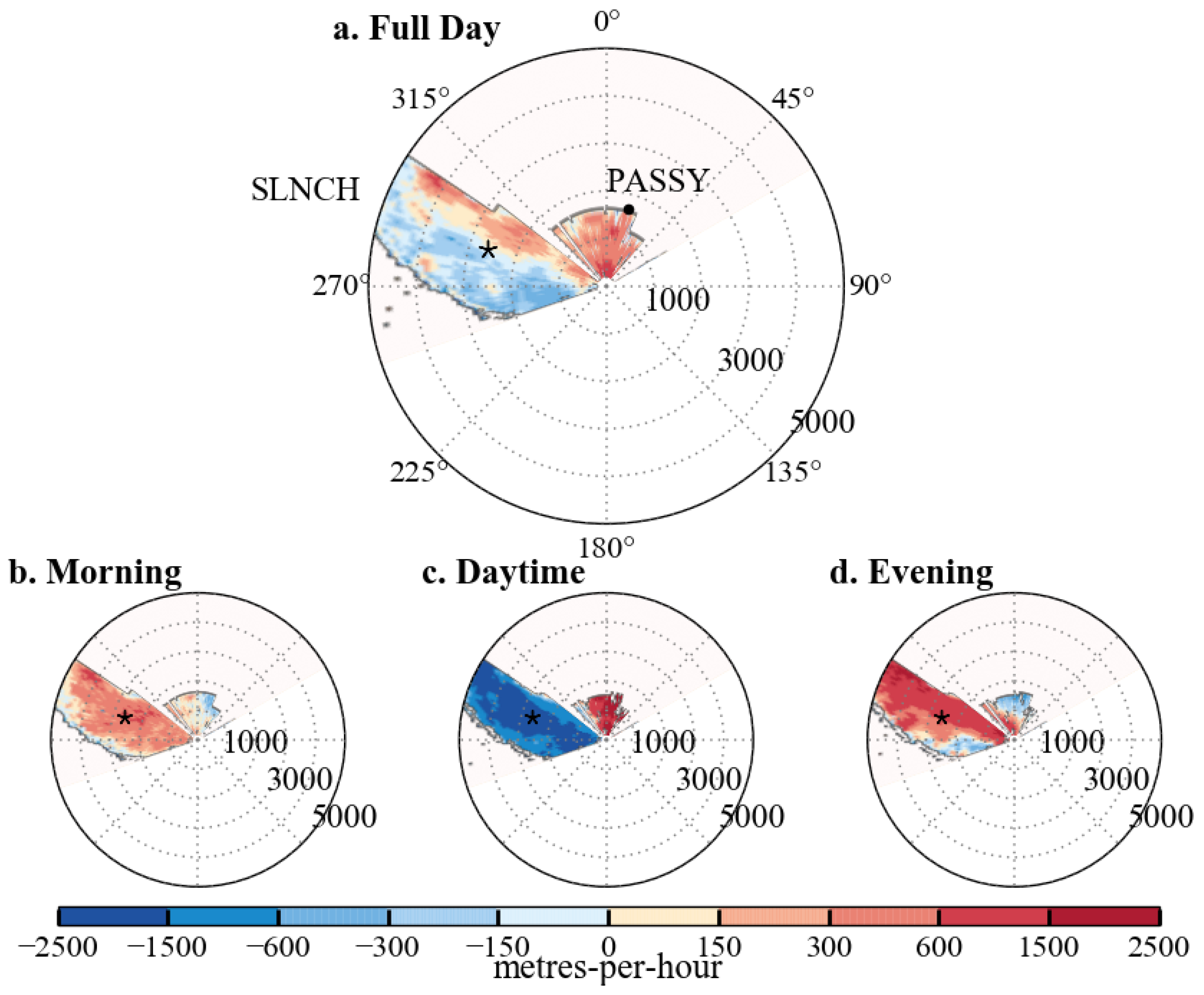
  • a northeast–southwest ventilation gradient observed when looking at the 24-h average with a westerly transport in the southern part of the basin and an easterly transport in the northern part of the basin, probably with more polluted air. This northeast–southwest gradient is consistent with the observed heterogeneity of the backscattered signal maps derived from the scanning DWL CNR signal.
To sum up, the complexity and very particular characteristics of the basin topography are mirrored in the local winds that are heterogeneous. Under stable wintertime conditions, the observed wind systems lead to an important variability in ventilation within the Passy basin. Instead of distributing the emissions among the valley, the wind system favors their accumulation in places where the highest PM10 concentrations are measured. This study finally highlights the importance of local dynamincs on PM10 distibution. Several questions regarding the mechanisms leading to the local wind structures observed arise from this work. A high resolution numerical modelling study is currently in progress in order to investigate these questions. The model has shown a good ability to represent the persistent temperature inversion dynamics observed during the first IOP [37]. Focus will now move to the role of the western part of the Passy basin, not covered by instruments during the field experiment, the Servoz passageway and its impact on the valley wind structures, and the possible role of the northern and southern slopes on the north–south local wind gradient. Particular attention will be paid to the elevated down-valley wind in the eastern part of the Passy basin as it appears to be a key element for the impact of local winds on air quality within the basin.

Acknowledgments

The Passy-2015 field experiment was supported by ADEME through the French national programme LEFE/INSU and by METEO-FRANCE. We thank the cities of Passy and Sallanches for their kind support. The field experiment was led by CNRM while LEGI is the principal investigator of the LEFE/INSU project. Data are managed by SEDOO at Observatoire Midi-Pyrénées (http://passy.sedoo.fr). We thank all the teams involved in the field experiment: GMEI/LISA, GMEI/4M, GMEI/MNPCA and GMEI/TRAMM at CNRM; LEGI, IGE, Atmo Auvergne-Rhone-Alpes and NCAS (UK). A special thanks to the people involved in the rawinsondes preparation and data acquisition under difficult meteorological conditions at night-time.

Author Contributions

T.S. wrote the paper and conducted the data analysis in the framework of her Ph.D. program. A.P. designed the scanning strategy of the lidar during the field experiment and helped in the interpretation of the results and manuscript revisions along with G.C. and Y.L.; A.P. brought its expertise on stable flows; G.C. brought its expertise on boundary layer dynamics; Y.L. largely contributed to the analysis of the dynamics of the temperature inversion episode; A.D. contributed to data-processing and supported the determination of the measurement accuracy. J.-M.D. and T.D. ensured the scanning Doppler wind lidar data acquisition during the field-experiment and helped on technical details and data-processing.

Conflicts of Interest

The authors declare no conflict of interest. The founding sponsors had no role in the design of the study; in the collection, analyses, or interpretation of data; in the writing of the manuscript, and in the decision to publish the results.

Appendix A. Speed Accuracy

The expected speed accuracy given by the manufacturer is less than 0.2 m·s 1 on V l o s measurements [39]. To make sure that this value was not affected by low wind conditions, it was checked in the conditions of use of the Passy-2015 field experiment by applying the correlation method described in Frehlich and Cornman [50]. This method decomposes the measured velocity v ^ ( k ) as v ^ ( k ) = v ( k ) + ϵ ( k ) , where v ( k ) corresponds to the “real” velocity and ϵ ( k ) the error. For each range gate, two correlation coefficients are computed, namely :
C ( 0 ) = 1 K k = 0 K 1 v ^ 2 ( k ) C ( 1 ) = 1 K 1 k = 0 K 2 v ^ ( k ) v ^ ( k + 1 ) .
The temporal average of the difference C ( 1 ) C ( 0 ) is then computed and associated with the corresponding mean CNR for the range gate. Assuming that v ( k ) and ϵ ( k ) are uncorrelated, that ϵ ( k ) is white noise and that the pulse repetition frequency is sufficiently large, the difference between the two correlation coefficients provides an estimation of the mean error C ( 0 ) C ( 1 ) ϵ 2 ( k ) .
The result is displayed in Figure A1. For C N R > 24 dB, the mean error on V l o s measures is around 0.12 m·s 1 (horizontal dotted line). Below 24 dB, the mean error increases when CNR decreases. Based one this consideration, we could use 24 dB as a threshold for the quality control of the data. However, the CNR distribution has a double Gaussian shape, with a first mode between 40 and 30 dB and a second one between 30 dB and 5 dB (not shown). The first mode corresponds to noise, whereas the other is associated with consistent signal data. As a result, the CNR threshold is fixed at 29 dB (vertical dashed line) in order to keep these significant data (which increases our database by 17 % ). Moreover, this 29 dB threshold is in agreement with the one derived from the heuristic semiempirical model proposed by Dabas [51] (not shown). In this way, we have more than 80 % of the database associated with a mean error of 0.12 m·s 1 and the remaining 20 % with a mean error of 0.27 m·s 1 . Since interactions of the laser beam with the motionless mountain sides are associated with high CNR, an upper CNR threshold is applied and set to 7 dB.
Figure A1. Estimation of the mean error as a function of CNR. The horizontal dotted line corresponds to the mean error for C N R > 24 dB. The vertical dashed line corresponds to the CNR threshold below which data are discarded.
Atmosphere 09 00118 g0a1

References

  1. Darby, L.S.; Allwine, K.J.; Banta, R.M. Nocturnal low-level jet in a mountain basin complex. Part II: Transport and diffusion of tracer under stable conditions. J. Appl. Meteorol. Climatol. 2006, 45, 740–753. [Google Scholar] [CrossRef]
  2. Gohm, A.; Harnisch, F.; Fix, A. Boundary Layer Structure in the Inn Valley during High Air Pollution (INNAP). In Proceedings of the 12th Conference on Mountain Meteorology, Santa Fe, NM, USA, 28 August– 1 September 2006; Available online: http://ams.confex.com/ams/pdfpapers/114458.pdf (accessed on 2 November 2017).
  3. Silcox, G.D.; Kelly, K.E.; Crosman, E.T.; Whiteman, C.D.; Allen, B.L. Wintertime PM2.5 concentrations during persistent, multi-day cold-air pools in a mountain valley. Atmos. Environ. 2012, 46, 17–24. [Google Scholar] [CrossRef]
  4. Rendón, A.M.; Salazar, J.F.; Palacio, C.A.; Wirth, V.; Brötz, B. Effects of urbanization on the temperature inversion breakup in a mountain valley with implications for air quality. J. Appl. Meteorol. Climatol. 2014, 53, 840–858. [Google Scholar] [CrossRef]
  5. Pope, C.A.; Dockery, D.W. Acute health effects of PM10 pollution on symptomatic and asymptomatic children. Am. Rev. Respir. Dis. 1992, 145, 1123–1128. [Google Scholar] [CrossRef] [PubMed]
  6. Laden, F.; Schwartz, J.; Speizer, F.E.; Dockery, D.W. Reduction in fine particulate air pollution and mortality: Extended follow-up of the Harvard Six Cities study. Am. J. Respir. Crit. Care Med. 2006, 173, 667–672. [Google Scholar] [CrossRef] [PubMed]
  7. Weinmayr, G.; Romeo, E.; De Sario, M.; Weiland, S.K.; Forastiere, F. Short-term effects of PM10 and NO2 on respiratory health among children with asthma or asthma-like symptoms: A systematic review and meta-analysis. Environ. Health Perspect. 2010, 118, 449. [Google Scholar] [CrossRef] [PubMed]
  8. Price, J.; Vosper, S.; Brown, A.; Ross, A.; Clark, P.; Davies, F.; Horlacher, V.; Claxton, B.; McGregor, J.; Hoare, J.; et al. COLPEX: Field and numerical studies over a region of small hills. Bull. Am. Meteorol. Soc. 2011, 92, 1636–1650. [Google Scholar] [CrossRef]
  9. Largeron, Y.; Staquet, C. Persistent inversion dynamics and wintertime PM10 air pollution in Alpine valleys. Atmos. Environ. 2016, 135, 92–108. [Google Scholar] [CrossRef]
  10. Whiteman, C.D. Mountain Meteorology: Fundamentals and Applications; Oxford University Press: Oxford, UK, 2000. [Google Scholar]
  11. Wagner, A. Theorie und Beobachtung der periodischen Gebirgswinde. [Theory and observation of periodic mountain winds]. Gerlands Beiträge zur Geophysik (Leipzig) 1938, 52, 408–449. [Google Scholar]
  12. Ekhart, E. De la structure thermique de l’atmosphère dans la montagne [On the thermal structure of the mountain atmosphere]. La Meteorologie 1948, 4, 3–6. [Google Scholar]
  13. Lehner, M.; Gohm, A. Idealised simulations of daytime pollution transport in a steep valley and its sensitivity to thermal stratification and surface albedo. Bound. Layer Meteorol. 2010, 134, 327–351. [Google Scholar] [CrossRef]
  14. Banta, R.; Olivier, L.; Neff, W.; Levinson, D.; Ruffieux, D. Influence of canyon-induced flows on flow and dispersion over adjacent plains. Theor. Appl. Climatol. 1995, 52, 27–42. [Google Scholar] [CrossRef]
  15. Colette, A.; Chow, F.K.; Street, R.L. A numerical study of inversion-layer breakup and the effects of topographic shading in idealized valleys. J. Appl. Meteorol. 2003, 42, 1255–1272. [Google Scholar] [CrossRef]
  16. Wagner, J.; Gohm, A.; Rotach, M. Influence of along-valley terrain heterogeneity on exchange processes over idealized valleys. Atmos. Chem. Phys. 2015, 15, 6589–6603. [Google Scholar] [CrossRef]
  17. Whiteman, C.D. Observations of thermally developed wind systems in mountainous terrain. In Atmospheric Processes Over Complex Terrain; Springer: Berlin, Germany, 1990; pp. 5–42. [Google Scholar]
  18. Blumen, W. Atmospheric Processes over Complex Terrain; Springer: Berlin, Germany, 1990; Volume 23. [Google Scholar]
  19. Salmond, J.; McKendry, I. A review of turbulence in the very stable nocturnal boundary layer and its implications for air quality. Prog. Phys. Geogr. 2005, 29, 171–188. [Google Scholar] [CrossRef]
  20. Largeron, Y. Dynamique de la Couche Limite Atmosphérique Stable en Relief Complexe. Application aux Épisodes de Pollution Particulaire des Vallées Alpines. Ph.D. Thesis, Université de Grenoble, Grenoble, France, 2010. [Google Scholar]
  21. Rucker, M.; Banta, R.M.; Steyn, D.G. Along-valley structure of daytime thermally driven flows in the Wipp Valley. J. Appl. Meteorol. Climatol. 2008, 47, 733–751. [Google Scholar] [CrossRef]
  22. Giovannini, L.; Laiti, L.; Seraphin, S.; Zardi, D. The thermally driven diurnal wind system of the Adige Valley in the Italian Alps. Q. J. R. Meteorol. Soc. 2017, 143, 2389–2402. [Google Scholar] [CrossRef]
  23. Doran, J.; Fast, J.D.; Horel, J. The VTMX 2000 campaign. Bull. Am. Meteorol. Soc. 2002, 83, 537–551. [Google Scholar] [CrossRef]
  24. Banta, R.M.; Darby, L.S.; Fast, J.D.; Pinto, J.O.; Whiteman, C.D.; Shaw, W.J.; Orr, B.W. Nocturnal low-level jet in a mountain basin complex. Part I: Evolution and effects on local flows. J. Appl. Meteorol. 2004, 43, 1348–1365. [Google Scholar] [CrossRef]
  25. Gohm, A.; Harnisch, F.; Vergeiner, J.; Obleitner, F.; Schnitzhofer, R.; Hansel, A.; Fix, A.; Neininger, B.; Emeis, S.; Schäfer, K. Air pollution transport in an Alpine valley: Results from airborne and ground-based observations. Bound. Layer Meteorol. 2009, 131, 441–463. [Google Scholar] [CrossRef] [Green Version]
  26. Harnisch, F.; Gohm, A.; Fix, A.; Schnitzhofer, R.; Hansel, A.; Neininger, B. Spatial distribution of aerosols in the Inn Valley atmosphere during wintertime. Meteorol. Atmos. Phys. 2009, 103, 223–235. [Google Scholar] [CrossRef] [Green Version]
  27. Duine, G.J.; Hedde, T.; Roubin, P.; Durand, P.; Lothon, M.; Lohou, F.; Augustin, P.; Fourmentin, M. Characterization of valley flows within two confluent valleys under stable conditions: Observations from the KASCADE field experiment. Q. J. R. Meteorol. Soc. 2017, 143, 1886–1902. [Google Scholar] [CrossRef]
  28. Atmo Auvergne-Rhone-Alpes. Available online: www.atmo-auvergnerhonealpes.fr (accessed on 12 December 2017).
  29. Paci, A.; Staquet, C.; Allard, J.; Barral, H.; Canut, G.; Cohard, J.M.; Jaffrezo, J.L.; Martinet, P.; Sabatier, T.; Troude, F.; et al. The Passy-2015 field experiment: Atmospheric dynamics and air quality. Poll. Atmos. 2016, 231–232. Available online: http://lodel.irevues.inist.fr/pollution-atmospherique/index.php?id=5903&format=print (accessed on 10 October 2017).
  30. Chemel, C.; Arduini, G.; Staquet, C.; Largeron, Y.; Legain, D.; Tzanos, D.; Paci, A. Valley heat deficit as a bulk measure of wintertime particulate air pollution in the Arve River Valley. Atmos. Environ. 2016, 128, 208–215. [Google Scholar] [CrossRef] [Green Version]
  31. PPA. Plan de Protection de l’Atmosphere (PPA) de la vallée de l’Arve. Available online: http://www.hautesavoie.gouv.fr/content/download/15754/92617/file/ppa_20120305.pdf (accessed on 12 December 2017).
  32. PPA. Le portail national de la connaissance du territoire mis en oeuvre par l’IGN. Available online: www.geoportail.gouv.fr (accessed on 1 June 2016).
  33. Air-Rhône-Alpes. Bilan de la Qualité de l’air 2015-Diagnostic Annuel; Technical Report; Air Rhône-Alpes: Lyon, France, 2015. [Google Scholar]
  34. Triantafyllou, A. PM10 pollution episodes as a function of synoptic climatology in a mountainous industrial area. Environ. Pollut. 2001, 112, 491–500. [Google Scholar] [CrossRef]
  35. Pernigotti, D.; Rossa, A.M.; Ferrario, M.E.; Sansone, M.; Benassi, A. Influence of ABL stability on the diurnal cycle of PM10 concentration: Illustration of the potential of the new Veneto network of MW-radiometers and SODAR. Meteorol. Z. 2007, 16, 505–511. [Google Scholar] [CrossRef] [PubMed]
  36. Schäfer, K.; Vergeiner, J.; Emeis, S.; Wittig, J.; Hoffmann, M.; Obleitner, F.; Suppan, P. Atmospheric influences and local variability of air pollution close to a motorway in an Alpine valley during winter. Meteorol. Z. 2008, 17, 297–309. [Google Scholar] [CrossRef]
  37. Largeron, Y.; Paci, A.; Rodier, Q.; Vionnet, V.; Legain, D. Persistent temperature inversions in the Chamonix-Mont-Blanc valley during IOP1 of the Passy-2015 field experiment. J. Appl. Meteorol. Climatol. submitted.
  38. Legain, D.; Bousquet, O.; Douffet, T.; Tzanos, D.; Moulin, E.; Barrié, J.; Renard, J.B. High-frequency boundary layer profiling with reusable radiosondes. Atmos. Meas. Tech. 2013, 6, 2195–2205. [Google Scholar] [CrossRef] [Green Version]
  39. Leosphere. WINDCUBE Product Information; Technical Report; Leosphere: Orsay, France, 2015. [Google Scholar]
  40. Fujii, T.; Fukuchi, T. Laser Remote Sensing; CRC Press: Boca Raton, FL, USA, 2005. [Google Scholar]
  41. Chouza, F.; Reitebuch, O.; Groß, S.; Rahm, S.; Freudenthaler, V.; Toledano, C.; Weinzierl, B. Retrieval of aerosol backscatter and extinction from airborne coherent Doppler wind lidar measurements. Atmos. Meas. Tech. 2015, 8, 2909–2926. [Google Scholar] [CrossRef]
  42. Courtney, M.; Wagner, R.; Lindelöw, P. Testing and Comparison of Lidars for Profile and Turbulence Measurements in Wind Energy; IOP Conference Series: Earth and Environmental Science; IOP Publishing: Bristol, UK, 2008; Volume 1, p. 012021. [Google Scholar]
  43. Kumer, V.M.; Reuder, J.; Furevik, B.R. A comparison of LiDAR and radiosonde wind measurements. Energy Procedia 2014, 53, 214–220. [Google Scholar] [CrossRef] [Green Version]
  44. Largeron, Y.; Staquet, C.; Chemel, C. Characterization of oscillatory motions in the stable atmosphere of a deep valley. Bound. Layer Meteorol. 2013, 148, 439–454. [Google Scholar] [CrossRef] [Green Version]
  45. Porch, W.M.; Fritz, R.B.; Coulter, R.L.; Gudiksen, P.H. Tributary, valley and sidewall air flow interactions in a deep valley. J. Appl. Meteorol. 1989, 28, 578–589. [Google Scholar] [CrossRef]
  46. McNider, R.T. A note on velocity fluctuations in drainage flows. J. Atmos. Sci. 1982, 39, 1658–1660. [Google Scholar] [CrossRef]
  47. Vergeiner, I.; Dreiseitl, E. Valley winds and slope winds—Observations and elementary thoughts. Meteorol. Atmos. Phys. 1987, 36, 264–286. [Google Scholar] [CrossRef]
  48. Etling, D. On plume meandering under stable stratification. Atmos. Environ. Part A Gen. Top. 1990, 24, 1979–1985. [Google Scholar] [CrossRef]
  49. Weigel, A.P.; Rotach, M.W. Flow structure and turbulence characteristics of the daytime atmosphere in a steep and narrow Alpine valley. Q. J. R. Meteorol. Soc. 2004, 130, 2605–2627. [Google Scholar] [CrossRef]
  50. Frehlich, R.; Cornman, L. Estimating spatial velocity statistics with coherent Doppler lidar. J. Atmos. Ocean. Technol. 2002, 19, 355–366. [Google Scholar] [CrossRef]
  51. Dabas, A. Semiempirical model for the reliability of a matched filter frequency estimator for Doppler lidar. J. Atmos. Ocean. Technol. 1999, 16, 19–28. [Google Scholar] [CrossRef]
Figure 1. Location of the Passy-2015 field experiment, in the Arve River Valley, close to Mont-Blanc (source: [32]). Mountain ranges are indicated in white upper case letters, and the three measurement sites used in this study in white lower case letters. The urbanized areas are represented by hatched zones, with a maximum housing density of 245 hab·km 2 in the Sallanches town. The Meteo-France automatic weather stations are indicated by yellow squares and the automatic TEOM-FDMS stations of the local air quality agency by blue stars. Green lines represent the baseline of the scanning lidar vertical scans. Adapted from [29].
Atmosphere 09 00118 g001
Figure 2. (a) time evolution of PM10 concentrations obtained by applying a 24 h-moving average on raw data recorded at four stations of the Arve river valley: Passy in red, Sallanches in orange, Chamonix in green and Marnaz in cyan. Grey areas represent PM10 pollution episodes based on Passy PM10 measurements; (b) time evolution of the sea level pressure measured in the middle of the Passy basin and at Annecy, in black and grey, respectively, and the temperature gradient between Sallanches and Mont-Arbois, in blue. Annecy, Sallanches and Mont-Arbois stations are the closest stations of the METEO-FRANCE operational network for both measurements. Black dots show the days for which albedo at Site 1 was above 0.5, i.e., the days with snow on the ground.
Atmosphere 09 00118 g002
Figure 3. Space and time (z,t) diagram of temperature obtained from high-frequency radiosoundings launched from the Passy basin centre (Site 1) during IOP1. Wind profiles are superimposed with wind direction given by the arrow orientation (a northerly wind points towards the bottom) and wind force given by the vector length.
Atmosphere 09 00118 g003
Figure 4. Scanning strategy of the WLS200S during the Passy-2015 field experiment. A horizontal PPI scan is represented in red, a slanted PPI scan at elevation 5° in black and the three vertical scans at azimuth 295°, 350°, 28° in green.
Atmosphere 09 00118 g004
Figure 5. Scatter plot comparing V l o s derived from the WLS8-5 lidar and measured by the WLS200S lidar during the IOP1 (974 values). The dashed line corresponds to the line 1:1 and the solid line represents the linear regression.
Atmosphere 09 00118 g005
Figure 6. Representation of the V l o s distribution for along- and cross-valley wind components for the January–February 2015 database in blue (Jan–Feb) and the stagnation stage of the IOP1 in red (10–12 Feb). The boxes represent the 25th and 75th percentiles, with a thick line representing median value, and the whiskers extending from the 1st to the 99th percentile. Positive (negative) V l o s represent a flow away from (toward) the lidar.
Atmosphere 09 00118 g006
Figure 7. Location within the Passy basin of the axes used to characterize the along-valley wind. The vertical profiles (green) are extracted from RHI scans 2000 m away from the lidar, the horizontal transect (red) is extracted from the PPI scan at elevation 0°. The cross-valley transects (blacks) are extracted from slanted PPI with elevation angle (ranging from 1° to 8°), in the centre (C) and in the east of the basin (E). The blue circular area is used to characterize the wind from the Saint-Gervais valley. Complete RHI and PPI scans can be seen in Figure 4.
Atmosphere 09 00118 g007
Figure 8. Space and time (z,t) diagrams of V l o s , extracted for a vertical profile (a) in the centre of the basin at azimuth 295° and (b) in the eastern part of the basin at azimuth 28°. Red corresponds to up-valley winds (approximately westerly in the basin centre) and blue to down-valley winds (approximately easterly). Altitude is given in metres above valley level as defined in Section 2.3.
Atmosphere 09 00118 g008
Figure 9. (a) space and time (x,t) diagrams of V l o s along the horizontal valley axis. Red corresponds to up-valley winds (approximately westerly in the basin centre) and blue to down-valley winds (approximately easterly). (b) mean and standard deviation of V l o s computed over the LOS distance, between 0 and 5 km, for each time step. Red stars represent the time step at which the wind in the along-valley direction is considered as heterogeneous based on the criterion defined below.
Atmosphere 09 00118 g009
Figure 10. Space and time (y,t) diagrams of V l o s over cross-valley transects extracted at elevation (a) 75 m; (b) 150 m; and (c) 250 m AVL in the central part of the Passy basin (transect C in Figure 7). Red corresponds to up-valley winds (approximately westerly in the basin centre) and blue to down-valley winds (approximately easterly). The axis of ordinates is given as the distance from the middle of the transect with positive y towards the north and negative y towards the south.
Atmosphere 09 00118 g010
Figure 11. The same as Figure 10 for cross-valley transects in the eastern part of the Passy basin (transect E in Figure 7), extracted at (a) 150 m and (b) 250 m AVL.
Atmosphere 09 00118 g011
Figure 12. Representation of the dominant away-from-lidar (red arrows) and toward-lidar (blue arrows) wind components blowing through the area delimited by an arc of a circle of radius 1000 m, 40 m AVL, represented in blue in Figure 7. Wind directions are given by the arrow orientations (a northerly wind points downwards) and wind force by the vector length. Each panel is associated with one day and grey areas indicate the time period during which southerly flows are observed.
Atmosphere 09 00118 g012
Figure 13. Horizontal maps of β T 2 derived from horizontal scans of CNR by applying the Equation (3) for four days of the persistent temperature inversion episode. The WLS200S is located at (0,0) and the black star indicates the location of Site 1 within the Passy basin. The black dot shows the location of the TEOM-FDMS station, which measured [ P M 10 ] at Passy. The Sallanches station (SLNCH) is out of the plot, 6.2 km away from the center in the the west–northwest direction, close to the southern sidewalls of the basin (blue star in Figure 1).
Atmosphere 09 00118 g013
Figure 14. Conceptual scheme of the main night-time wind structures observed from WLS200S measurements within the Passy basin. Blue (red) arrows represent down-valley (up-valley) flows. Wind oscillations are represented by the hatched red and blue wave. Dotted arrows represent the flows observed intermittently during the night. The tributary valley locations are indicated in capital letters and the main towns within the Passy basin in lower-case letters.
Atmosphere 09 00118 g014
Figure 15. Horizontal map of ventilation index obtained from PPI scan, 40 m AVL for (a) the full 11 February, (b) the early morning stage [0:00 a.m.:10:59 a.m.] UTC; (c) the daytime stage [11:00 a.m.:4:59 p.m.] UTC; and (d) the evening stage [5:00 p.m.:11:59 p.m.] UTC. Blue represents ventilation in the toward-lidar LOS direction and red represents ventilation away-from-lidar, which is located at the centre (0,0). The black star indicates the location of Site 1 within the Passy basin and the black dot shows the location of the TEOM-FDMS station, which measured [ P M 10 ] at Passy. The Sallanches station (SLNCH) is out of the plot, 6.2 km away the center in the west–northwest direction, close to the southern sidewalls of the basin (blue star in Figure 1).
Atmosphere 09 00118 g015
Table 1. Pollution episodes during the winter 2015 in the Arve River Valley. The maximum daily [ P M 10 ] (in μ g·m 3 ) recorded during the episode for the stations of Passy, Sallanches and Chamonix are given together with the day during the episode at which this maximum was reached (in parentheses).
EpisodeTimeMax [ PM 10 ] Passy (Day of the Max/Epis. Duration)Max [ PM 10 ] Sallanches (Day of the Max/Epis. Duration)Max [ PM 10 ] Chamonix (Day of the Max/Epis. Duration)
11–8 January115 ( 6 / 8 )60 ( 6 / 8 )60 ( 1 / 8 )
217–22 January98 ( 4 / 6 )48 ( 4 / 6 )37 ( 5 / 6 )
39–14 February88 ( 3 / 6 )73 ( 3 / 6 )48 ( 1 / 6 )
416–20 February66 ( 2 / 5 )54 ( 2 / 5 )61 ( 3 / 5 )
Table 2. Description of the sites shown in Figure 1 with their geographical coordinates, their elevation in metres Above Sea Level (m ASL) and in metres Above Valley Level (m AVL). The instruments used in this study are described along with the parameters measured, the measurement geometry (Z refers to vertical profile, H to horizontal profile and L to local measurement) and the period at which measurements are available.
SiteCoord. (N, E)Elev. (m ASL)Elev. (m AVL)SensorVariablesMeas. Geom.Meas. Available Every
145.9140
6.6741
5600Profiler Doppler Wind Lidar WLS8-5 (Leosphere)DD, FF, CNRZ3 s
Radiosonde RS92-SGP (Vasaila)T, RH, DD, FFZ3 h
Ceilometer CT25K (Vaisala)Cloud layer bottomZ15 s
Net Radiometer CNR1 (Kipp and Zonen) S W , S W L30 min
Present Weather Detector PWD22 (Vaisala)VisibilityL14 s
Barometer PTB210 (Vaisala)PL1 min
245.9080
6.7072
60242Scanning Doppler Wind Lidar WLS200S (Leosphere) V l o s , CNRZ
H
30 min
10 min
345.9235
6.7136
58828TEOM-FDMS (Thermo Fisher Sci.)PM10L1 h
Table 3. Characteristics of the 3D long range Doppler wind lidar WLS200S and profiler Doppler wind lidar WLS8-5 (both designed by Leosphere) used during the Passy-2015 field experiment.
WLS200SWLS8-5
Wavelength ( μ m) 1.54 1.54
Accumulation time (sec)13
Nb. Pulses averaged 10 , 000 30 , 000
Scan speed (deg·s 1 )1-
Range resolution (m)10020
Range gates5924
Azimuth Range (°relative to north)250 to 60-
Elevation Range (°relative to Horiz.)0 to 90-
Scan cone angle (°)- 14.93
Speed accuracy (from manufacturer) (m·s 1 ) 0.2 0.1
Direction accuracy (from manufacturer) (°)-2

