Understanding Long-Term Variations in Surface Ozone in United States (U.S.) National Parks


1
Department of Chemistry, State University of New York College of Environmental Science and Forestry, Syracuse, NY 13210, USA
2
Department of Earth, Ocean and Atmospheric Science Florida State University Tallahassee, FL 32306, USA
3
National Park Service, Air Resources Division, Lakewood, CO 80235, USA
4
Clean Air Markets Division, United States Environmental Protection Agency, Washington, DC 20460, USA
*
Author to whom correspondence should be addressed.
Atmosphere 2018, 9(4), 125; https://doi.org/10.3390/atmos9040125
Submission received: 6 February 2018
/
Revised: 13 March 2018
/
Accepted: 17 March 2018
/
Published: 25 March 2018
(This article belongs to the Section Air Quality)
Abstract
:Long-term surface ozone observations at 25 National Park Service sites across the United States were analyzed for processes on varying time scales using a time scale decomposition technique, the Ensemble Empirical Mode Decomposition (EEMD). Time scales of interest include the seasonal cycle, large-scale climate oscillations, and long-term (>10 years) trends. Emission reductions were found to have a greater impact on sites that are nearest major urban areas. Multidecadal trends in surface ozone were increasing at a rate of 0.07 to 0.37 ppbv year−1 before 2004 and decreasing at a rate of −0.08 to −0.60 ppbv year−1 after 2004 for sites in the East, Southern California, and Northwestern Washington. Sites in the Intermountain West did not experience a reversal of trends from positive to negative until the mid- to late 2000s. The magnitude of the annual amplitude (=annual maximum–minimum) decreased at eight sites, two in the West, two in the Intermountain West, and four in the East, by 5–20 ppbv and significantly increased at three sites; one in Alaska, one in the West, and one in the Intermountain West, by 3–4 ppbv. Stronger decreases in the annual amplitude occurred at a greater proportion of sites in the East (4/6 sites) than in the West/Intermountain West (4/19 sites). The date of annual maximums and/or minimums has changed at 12 sites, occurring 10–60 days earlier in the year. There appeared to be a link between the timing of the annual maximum and the decrease in the annual amplitude, which was hypothesized to be related to a decrease in ozone titration resulting from NOx emission reductions. Furthermore, it was found that a phase shift of the Pacific Decadal Oscillation (PDO), from positive to negative, in 1998–1999 resulted in increased occurrences of La Niña-like conditions. This shift had the effect of directing more polluted air masses from East Asia to higher latitudes over the North American continent. The change in the Pacific Decadal Oscillation (PDO)/El Niño Southern Oscillation (ENSO) regime influenced surface ozone at an Alaskan site over its nearly 30-year data record.
1. Introduction
High concentrations of tropospheric ozone can have adverse effects on human health and vegetation. The United States (U.S.) Environmental Protection Agency (EPA) recently lowered the National Ambient Air Quality Standard (NAAQS) for ozone from 75 ppbv to 70 ppbv [1,2], in 2015. To attain the ozone NAAQS, a monitor’s fourth-highest annual daily maximum 8-h average ozone concentration (DM8HA) averaged over three consecutive years (i.e., the monitor’s design value) must not exceed 70 ppbv [1,2]. Regional emission controls for nitrogen oxides (NOx) have aided in the decrease of summertime ozone in the eastern U.S. as well as parts of California [3,4]. There are concerns that the influx of East Asian emissions [5,6,7], and the influences by interannual and interdecadal variability in the El Niño Southern Oscillation (ENSO) and the Pacific Decadal Oscillation (PDO) may make ozone attainment difficult for regions of higher elevation in the western U.S. [6,8,9,10]. Meeting and maintaining lower ozone standards may also be more difficult in a warming climate [11]. A quantitative understanding of the spatiotemporal variability in observed ozone on time scales of days to decades can assist policy makers in developing effective mitigation strategies for ozone abatement.
Regional U.S. ozone control strategies have successfully decreased DM8HA ozone in the eastern U.S., California, and the Intermountain West at the 95th, 50th, and 5th percentiles in the summer months [7]. Similar decreases in the DM8HA ozone was found in spring, at the 95th and 50th percentile, but at fewer sites across the U.S. [7,9]. However, increases at the 5th percentile were observed in most regions in springtime [7,9]. Recently, a leveling of the mean trend, followed by a slight decrease has been observed in the Pacific Northwest [12]. In addition to these observed changes, model simulations indicated that the springtime transport of East Asian pollution enhanced surface ozone at western U.S. sites by about 5 ppbv [13,14] and by up to 8–15 ppbv during high pollution episodes [14]. Transport of ozone precursors from East Asia may be linked to increases in springtime ozone concentrations in portions of the western U.S. However, the transport of East Asian emissions varies with the transport pathway that is facilitated by large-scale circulation patterns, which may affect ozone concentrations on time scales of days to decades [7,8].
The effect of ENSO and PDO on ozone has been identified previously in both model and observation-based studies. ENSO and PDO influenced the origin and fate of air masses that are arriving to the U.S. [10,15]. Using an observation-based approach, Langford et al. [16] found that the effect of ENSO on ozone was largely dependent on the strength of the ENSO event in the Western U.S., and that ozone was anticorrelated with the Southern Oscillation Index (SOI). While using a model based approach, Koumoutsaris et al. [17] and Lin et al. [8] found that ozone transported to the northern mid-latitudes was enhanced in spring following an El Niño event and diminished following a La Niña event. Lin et al. [8] also suggested that transpacific transport of East Asian emissions to the western U.S. decreased after 1998 following a shift in the PDO phase from positive to negative. The negative phase of PDO is concurrent with a La Niña event, which shifts the subtropical jet stream to the north, thereby weakening transport of ozone-rich air from East Asia to the central west coast of the U.S., subsequently decreasing the transport of East Asian pollutants across the southern U.S. [8]. During peak La Niña periods, ozone-rich air was preferentially transported to the Pacific Northwest, thereby enhancing ozone concentrations to this area [8]. The peak phases of these climate modes potentially altered the timing, frequency, and magnitude of pollutant influx entering the western U.S. This, as well as regional ozone control standards, is believed to have played a role in the timing and magnitude of maximums and minimums of the annual ozone cycle across the northern mid-latitudes [18,19,20]. The effect of these large-scale climate processes on surface ozone has yet to be sufficiently investigated and quantified using observation-based approaches.
Tropospheric ozone records show a pronounced seasonal cycle with peaks in late spring to summer and minimums in late fall to winter, which is largely driven by the photochemical production of ozone and temperature [21,22]. Monitoring sites in and around urban areas tend to have a mid-summer ozone peak resulting from maximum photochemical production during this season [23]. On the other hand, some high-elevation remote regions experience a late spring ozone maximum that is associated with stratospheric intrusions and hemisphere-wide photochemical production at this time of year [18,19,20]. Significant increases in springtime free tropospheric ozone over North America have been thought to largely result from the transport of polluted air masses from East Asia [9,24]. In addition, decreasing NOx emissions in the northern mid-latitudes of Europe have resulted in less ozone titration by NO in early spring, further leading to a shift in the ozone annual maximum to earlier in the year [18,25]. At five sites in Europe and North America, peaks in the ozone seasonal cycle have shifted earlier by three to six days per decade; this trend was explained by changes in atmospheric dynamics, which may have aided in the change in distribution of precursor emissions throughout the year. Increased westerly flow related to changes in the North Atlantic Oscillation (NAO) in the 1980s and 1990s may have increased pollution levels and subsequently, ozone in the spring and winter months across the northern mid-latitudes [18]. Cooper et al. [26] focused on 8 sites between the U.S. and Europe, and found that between 1990 and 2010, five sites had peak ozone occurring 1–3 months earlier in the year. A systematic study is needed to understand how various long-term processes impact ozone on multiple timescales across the U.S. by using remote sites over the entire period of availability of ozone data sets.
Therefore, this study focuses on ozone trends from National Park Service sites as the remote locations of many of these sites are ideal for studying the long-term variation in surface ozone. Here, we examine ozone observations between 1983 and 2015 at 25 National Park sites that are operated by the U.S. National Park Service (NPS). The Ensemble Empirical Mode Decomposition (EEMD) method [27] was employed to analyze ozone on multiple temporal scales. When compared to other data analysis methods that are commonly used in the literature, EEMD is unique in its nonlinear trend assessment and more economic computing time.
2. Data and Methods
The data used in this study were collected by the NPS Gaseous Pollutant Monitoring Program (NPS GPMP) (http://ard-request.air-resource.com/) [28]. Ozone is the primary gas monitored throughout the network that follows all the EPA protocols and is certified annually by the NPS to the EPA. The certification is supported by the Quality Assurance Project Plan (QAPP) [29], which specifically addresses the procedures used by the NPS to operate and certify ozone measurements at NPS-operated sites with EPA-certified analyzers. The data sets used here were all acquired from regulatory ozone monitoring stations; the sampling methods for gaseous and meteorological monitoring are based on the 40 CFR Part 58 requirements. All GPMP ambient ozone data is processed through several layers of rigorous validation by staff analysts. To ensure that each GPMP site and ozone monitor is operating properly and calibrated correctly, the full suite of GPMP network data are reviewed daily by a different independent analyst [29]. All data analysts all of which follow the same quality assurance/quality control (QA/QC) protocols that are set by the QAPP [29]. Bias and error in the data are determined by finding the deviation from the “true value” as a percentage of the true value [29]. Data analysts also monitor the amount of valid data acquired from each site and compare it to the expected amount under normal conditions in order to assess that data completeness criteria requirements are either met or to immediately identify a problem at a site. Additionally, the comparability of the data sets are monitored to ensure all final validated data is meaningfully comparable. Data validation for the entire GPMP network is performed monthly and uploaded to the EPA Air Quality System (AQS) database and is made available on the NPS Data Request web page. Further details regarding site operation and data processing can be found in the GPMP QAPP [29].
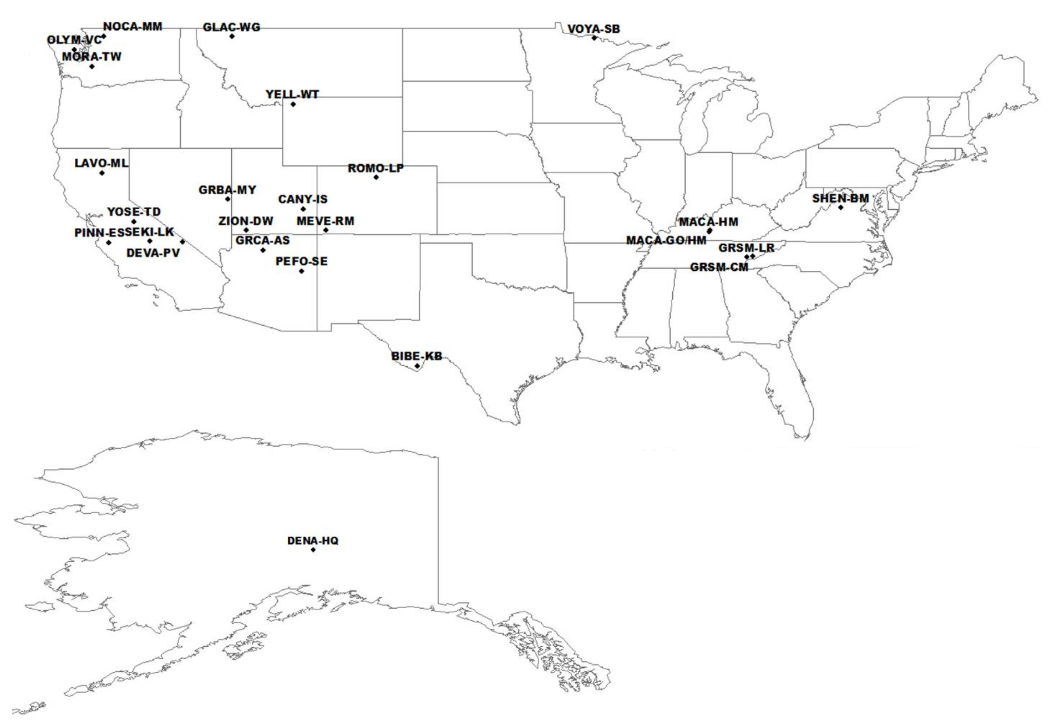
To study the variability of ozone on decadal to interdecadal time scales, all of the data sets used in this work had a minimum length of ten years. The locations and information for each site can be found in Table 1 and Figure 1. A total of 25 sites were available for this study which span time periods over 1983–2015. Of the sites used, six sites are in the eastern U.S., 18 are in the West and Intermountain West, and one is in Alaska. All of the sites are effectively far from urban centers and are representative of a well-mixed atmosphere. Please note that the data series for ROMO-LP, in Colorado, started in 1987 however, between 1987 and 1997, 39% of the data during this period was missing. After this period, incomplete data dropped dramatically, with only 5% missing data between 1998 and 2015. Completeness of a data series is also a requirement for accurate EEMD results. Therefore, data at this site was analyzed beginning in January 1998.
For the assessment of variability in these data, the EEMD method [27] is used. The algorithm decomposes a time series into the temporal signals that make up its total variability. Specifically, a time series is broken down into k oscillatory components where components of higher frequency are extracted first. The oscillatory components or signals, are referred to as Intrinsic Mode Functions (IMFs). The number of IMFs of a dataset was estimated to be log2N-1 [27,30], where N is the number of data points, which, in our case, was daily data averaged from hourly data. Component IMFs obey two properties: (i) the number of local maxima and minima differ at most by 1, and (ii) an IMF has a mean value of zero. The sifting process is repeated until the mean of the signal is sufficiently close to zero. After all of the signals are extracted from the time series, the residual (Rn) of the raw data results.
It is important to note that for shorter time series such as ZION-DW and NOCA-MM, 12 components were identified using EEMD. However, the variance associated with the components is very small given that longer-term components do not complete a full oscillation due to lack of an extended data series. Therefore, data that is unable to be decomposed into components will end up in the residual and add to the trend. The percent variance that is contributed by longer components such as 11 and 12 is well under a percent. Therefore, these long-term components do not contribute significant uncertainty to the overall trend of shorter data sets.
The time derivative of Rn was calculated to determine the long-term trend in ozone at each site and the date on which the ozone trend changed, if at all. The trends resulting from the EEMD method are representative of the trends depicting ozone impacted by processes on multidecadal times scales. Some of the main factors that could have influenced ozone on multidecadal timescales include the effect of regional ozone controls, land use and cover change, natural climate variability, and the 11-year solar cycle. It must be pointed out that this trend differs from the trends in baseline or background ozone that have been studied extensively in the current literature. The U.S. Environmental Protection Agency defines Policy Relevant Background (PRB) ozone as those concentrations that would occur in the U.S. in the absence of anthropogenic emissions in continental North America [31]. Background ozone needs to be quantified with the use of atmospheric models [31]. Baseline ozone is defined as ozone that has not been influenced by recent, locally emitted, or produced pollution [31]. Per the definition of background ozone and baseline ozone, both can be impacted by processes on time scales of days to years, and certainly bear seasonal to interannual variations. In the literature, trends in background ozone reflect the trends in model simulated influence from outside of the study domain, which excludes changes in all sources, sinks, and processes inside the study domain, and is also affected by model uncertainties [7,14]. Trends in baseline ozone are measurement-based, but are mostly a singular trend, or lack thereof, for the entire study period. In comparison, the trend resulting from the EEMD method is one that does not include processes on time scales that are shorter than 10 years, and there could be more than one trend within the study period. To distinguish from the baseline or background trend in the literature, the trend that is identified in this study is referred to as the multidecadal trend.
To investigate the impact of atmospheric dynamics on ozone, we used gridded datasets from the European Center for Medium Range Forecasts (ECMWF) (http://www.ecmwf.int/) [32], including monthly 2.5° × 2.5° gridded reanalysis fields of zonal and meridional winds, as well as 500 hPa geopotential height for the study period 1987–2015. We also used the NOAA Hybrid Single Particle Lagrangian Integrated model (HYSPLIT) dispersion version [33] to identify the origin of air masses of interest driven by NCEP/NCAR 2.5° × 2.5° meteorological data.
3. Results
The ozone data were decomposed into 12 oscillatory components using EEMD. For this study, we will focus on three of these components, including the 7th, 9th, and 10th component, and the residual, which were referred to as C7, C9, C10, and Rn, respectively. Our components of interest vary annually, interannually (by ENSO and PDO), and, as mentioned in Section 2, the residual Rn is the multidecadal variability. The components of interest at one site, ROMO-LP, are shown in Figure 2 as an example of EEMD results.
3.1. The Multidecadal Trend
The multidecadal trend in ozone, reported as the mean rate of change and one standard deviation before and after the date of trend change for each site can be found in Table 2, and the spatial variability in trends can be found in Figure 3.
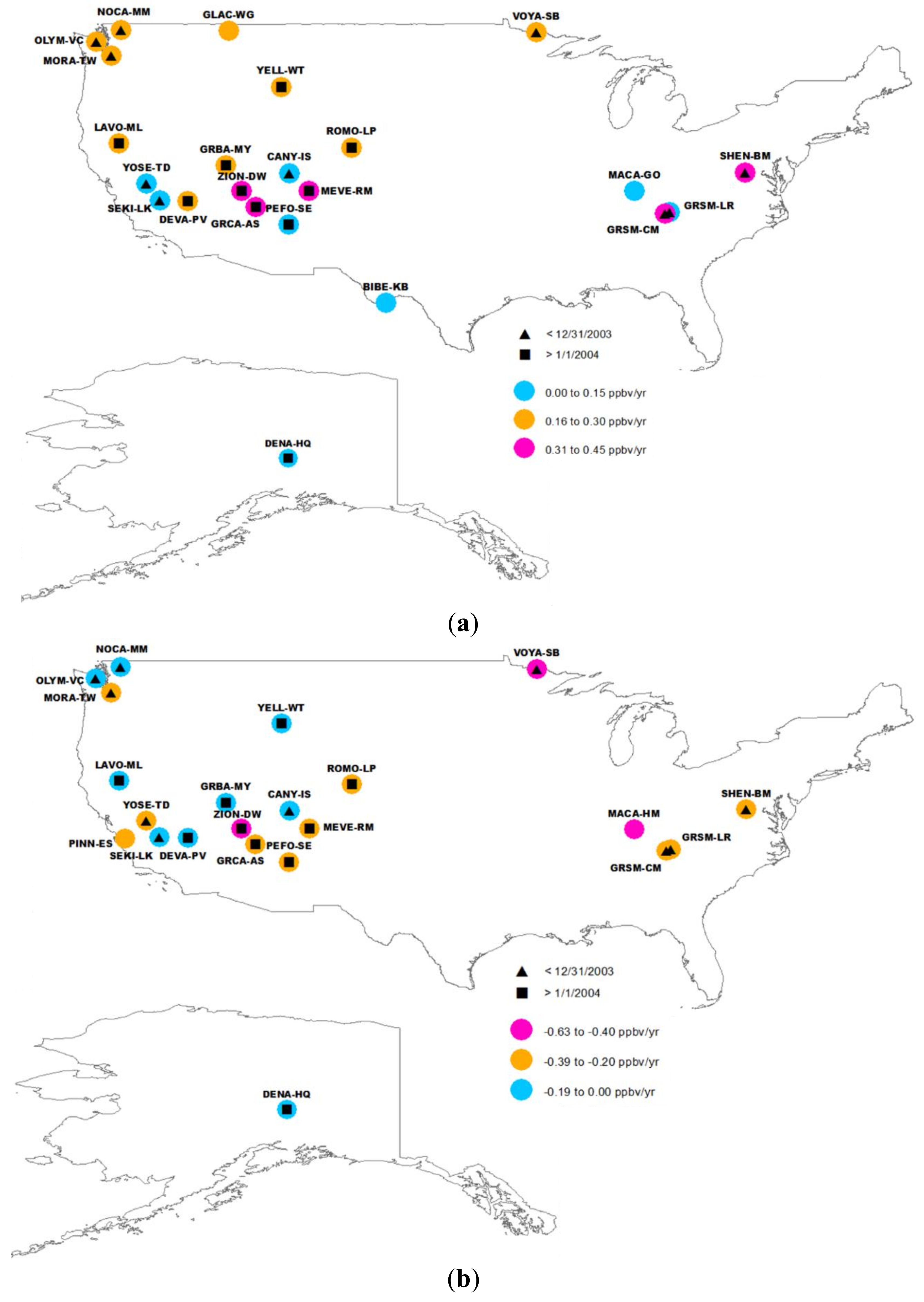
It is worth noting that the trends at 20 out of the 25 sites changed from positive to negative at some point in time during the study period, and a clear divide in the date of the trend change was observed. Additionally, the trends at sites in closer proximity to regions of higher population changed before 2004, while those at sites in the West and Intermountain West changed during or after 2004. Therefore, the rates of positive and negative trends were identified with the date of trend change as occurring either before 31 December 2003 or after 1 January 2004. The monitoring at MACA-GO ended in 1997 and was replaced by MACA-HM, which is seven miles away, in the same year; therefore, trends in this region were considered to have changed from increasing to decreasing in the year 1997. Excluding MACA-GO, two sites exhibited constant increasing trends (BIBE-KB (TX) and GLAC-WG (MT)), and one with a constant decreasing trend (PINN-ES (CA)).
Of the sites in the western half of the U.S., positive trends were the lowest mostly in Central California and Texas, ranging from 0.07 to 0.11 ppbv year−1, while stronger positive trends of 0.37–0.44 ppbv year−1 were found largely in the Intermountain West at GRCA-AS, MEVE-RM, and ZION-DW (Figure 3a). Trends in the West changed from positive to negative over a broad range of time, between 1997 and 2008 (Table 2). Within that time period, three sites changed from positive to negative prior to 2004 and nine sites after 2004. Ozone levels have been trending downward at 17 of the 19 western sites at rates that range between −0.02 to −0.63 ppbv year−1, since their respective dates of trend change (Table 2). The strongest negative trends in the West were found at ZION-DW at −0.63 ppbv year−1, followed by PINN-ES, at −0.34 ppbv year−1. Note that PINN-ES exhibited a constant decreasing trend averaging −0.34 ppbv year−1 throughout its monitoring period (1987–present). Trends at SEKI-LK and YOSE-TD, located in the west, changed from positive to negative in 1997 and 1998, respectively, marking these two sites the second and third to change their trend status from positive to negative, while GRSM-CM, located in the east, changed trends status in 1995, marking this as as the first site, to change its trend status from positive to negative. CANY-IS, which is located in southeastern Utah, is the fourth site to shift to negative prior to 2004 and is the only site in the intermountain West to change trend status from positive to negative prior to 2004. Of the nine sites with a change from positive to negative after 2004, all but CANY-IS are located in the Intermountain West, excluding LAVO-ML, which is located in northern California.
At GLAC-WG (MT) and BIBE-KB (TX), ozone trends have been increasing at 0.18 and 0.11 ppbv year−1 since the start of monitoring in 1992 and 1990, respectively. Both of these sites have exhibited a leveling of ozone trends beginning in 2014, but neither site has shown a reversal of trends. DENA-HQ had a weakly positive trend of 0.04 ppbv year−1 between 1987 and 2006, at which point the trend shifted downward at a rate of −0.02 ppbv year−1. In the East, trends at all of the sites changed from positive to negative prior to 2004. Rates of positive trends ranged from 0.07 ppbv year−1 at GRSM-CM to 0.35 ppbv year−1 at GRSM-LR. GRSM-CM had a trend shift from positive to negative the earliest of all sites, but also had the weakest positive trend. Since 2004, ozone has been trending downward at all five of the eastern sites (MACA-GO is no longer monitoring). Overall, surface ozone levels are decreasing at 22 of the 25 NPS sites across the U.S.
3.2. The Seasonal Cycle
The ozone seasonal cycle (C7), considered to be changing with the seasons but having one peak and one minimum per year, has varied in timing and amplitude at several sites. The most distinctive feature of the seasonal cycle is the spring/summer maximum and fall/winter minimum at all sites, which is characteristic of the Northern Hemisphere [21,22,34]. DENA-HQ has a very different seasonal cycle from the other sites in the study domain, with maxima in late March and minima in late August. Of all the components, the seasonal cycle contributed the greatest, 31.8% on average, of the total variance. Therefore, the seasonal cycle is the most important characteristic of the data controlling variation in ozone.
3.2.1. Change in Amplitude of Seasonal Cycles
The annual amplitude is the difference in ppbv between the annual ozone maximum and minimum. The magnitude of annual amplitude decreased significantly (p < 0.10) by 5 to 20 ppbv at four sites in the West and four sites in the East during their respective monitoring periods (Figure 4a,b; Table 1). Amplitude decreases in the West ranged between 5–7 ppbv for all four sites (Figure 4a), while the sites in the East have decreased by 5 ppbv at MACA-GO, 10 ppbv at MACA-HM, and 20 ppbv at GRSM-CM and SHEN-BM during their respective monitoring periods (Figure 4b). Stronger amplitude decreases were observed in the East than in the West, and proportionately more sites experienced decreases in the East than the West. Three sites had significant increases in annual amplitude, none of which were located in the East (Figure 4c). Specifically, LAVO-ML, which is located in northern California, had an increase of 3 ppbv between 1987 and 2015. DENA-HQ had an increase of 4 ppbv over the same time-period. GLAC-WG had an overall increase of 3 ppbv between 1992 and 2015. In comparison, sites with increases in annual amplitude were not as significant in magnitude as sites with decreases in annual amplitude.
3.2.2. Change in Timing of Seasonal Cycles
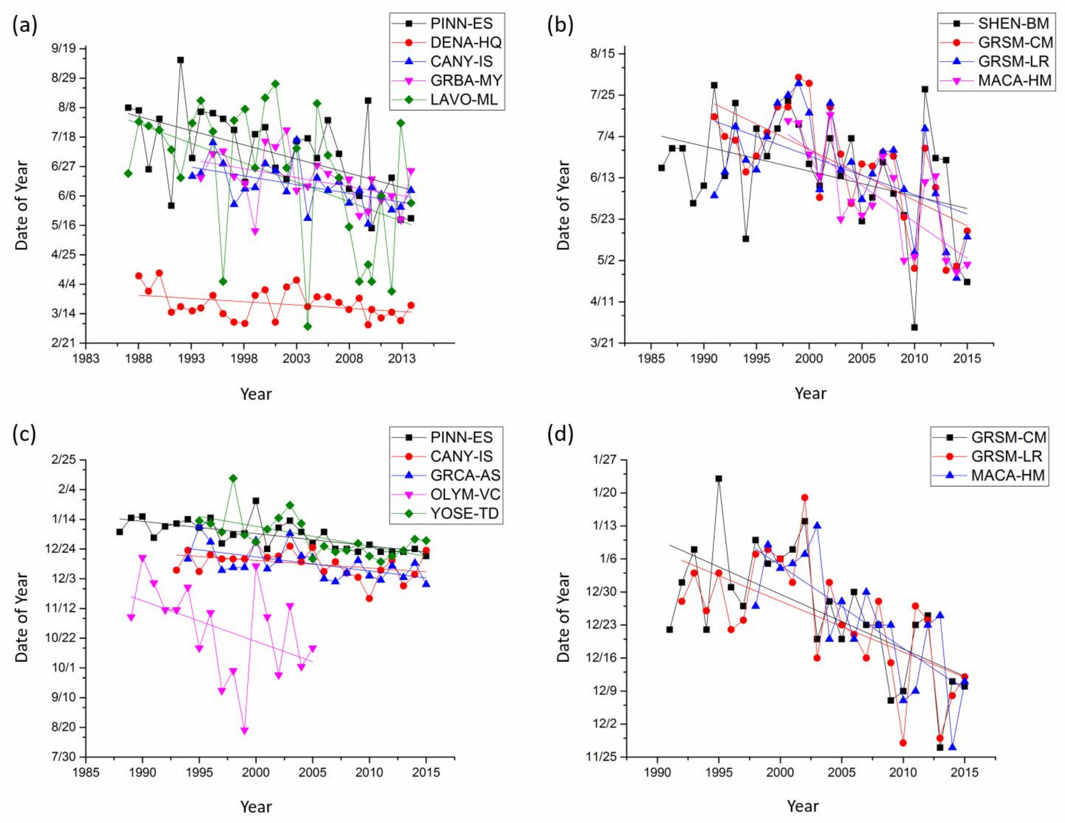
A shift to earlier in the year was observed in the annual maximums and minimums at 17 of the 25 sites. Sites with a significant shift are indicated in Figure 5. Figure 5a,b depict the nine sites that had a significant shift in peak date with 5 in the West, including the one site in Alaska (DENA-HQ) (Figure 5a), while Figure 5b shows four sites in the East. The sites with significant peak shifts in the West had shifted 10 to 60 days earlier during their respective monitoring periods (Figure 5a), while in the East, sites have moved 35 to 60 days earlier (Figure 5b). A closer examination revealed that the annual peaks at eight of the nine sites occurred in June and July prior to 2000, but afterward gradually shifted to late April/early May (Figure 5a,b). The annual maxima at DENA-HQ in Alaska shifted earlier by 10 days from early April in 1987 to late March beginning around 2003 (Figure 5b). Eight sites had an earlier occurring annual minimum, while four of these sites also had a shifting annual maximum (Figure 5c,d). Five of the eight sites with shifting annual minima were in the West, while the other three reside in the East. The annual minimum shift was more significant in the three eastern sites (28–34 days) than the five western sites (14–21 days).
Proportionately more sites in the East had a shift in the seasonal cycle than in the West for both the annual maximum and minimum. Of the nine sites with significant (p < 0.10) changes in the annual amplitude, six had significant (p < 0.10) changes in the date of annual maximums and minimums (SHEN-BM, GRSM-CM, MACA-HM, PINN-ES, DENA-HQ, CANY-IS, LAVO-ML), while three had insignificant (p > 0.10) shifts to an earlier date (GRSM-LR, MACA-GO, GRBA-MY). Conversely, only three sites with significant changes in amplitude had significant shifts in the minimum date (PINN-ES, GRSM-CM, and MACA-HM).
3.3. Variability by Large-Scale Climate Circulation Linked to Components C9 and C10
Surface temperature data have been widely analyzed and its time scales have been identified in the literature [10,35,36]. Zhang et al. [36] examined the correlation of the Precipitation Condition Index, Vegetation Condition Index, and decomposed precipitation and temperature data with the Niño 3.4 SST index. They identified the lag and correlation coefficient between this climate mode and the components representing ENSO to determine if ENSO was the main driver of variability [36]. However, the correlation and lag response of a variable that is associated with PDO is not as clear. Therefore, given the robustness of EEMD and the suggested linkage between ENSO/PDO and surface temperature [35,37], surface temperature data were decomposed by EEMD for each site and was used as a proxy to determine if there was a similar linkage between ENSO/PDO and surface ozone. The EEMD time scales for components 9 and 10 for temperature oscillate every 3–7 years and 9–12 years, respectively, which match with the variability identified for ENSO and PDO [38,39].
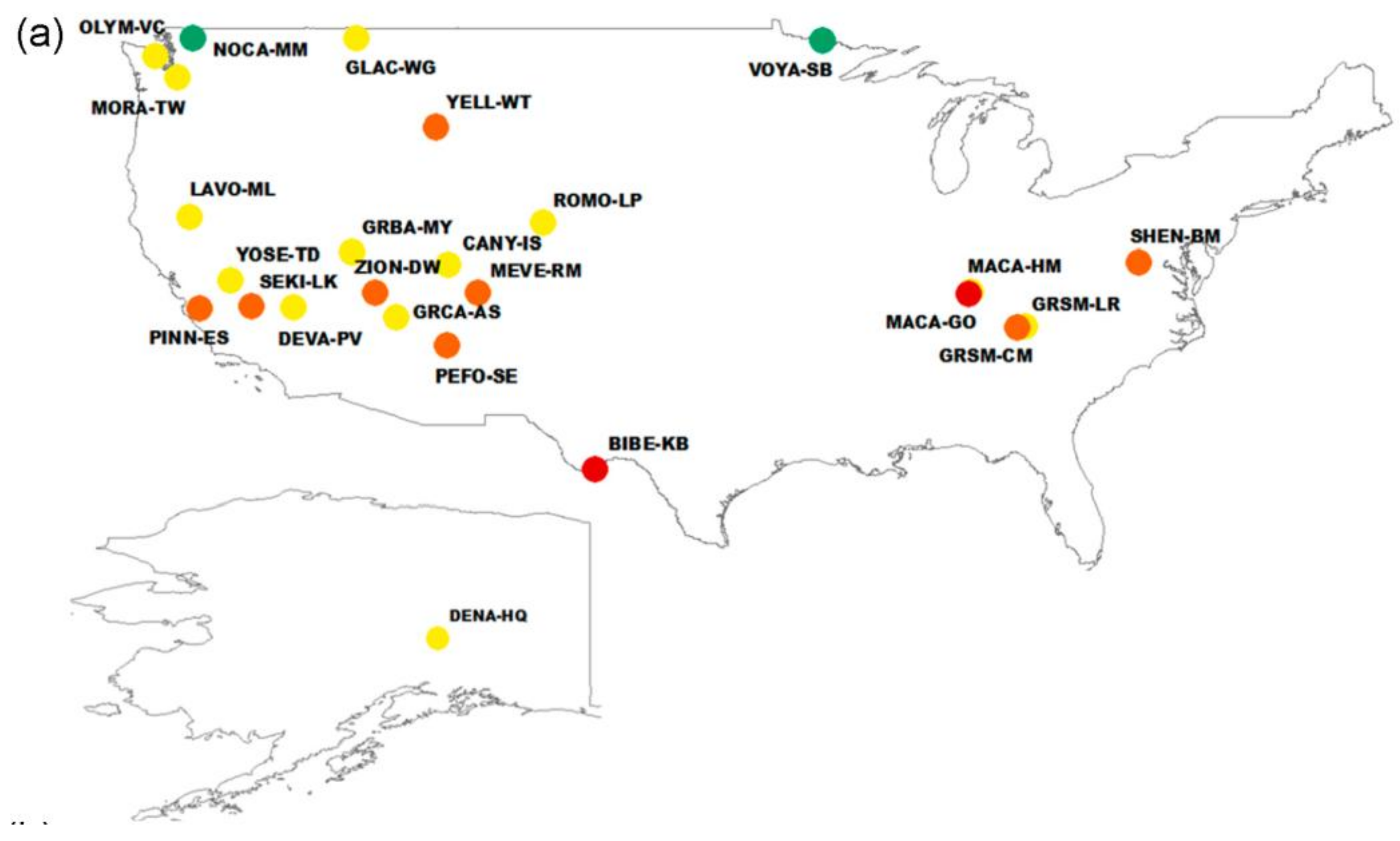
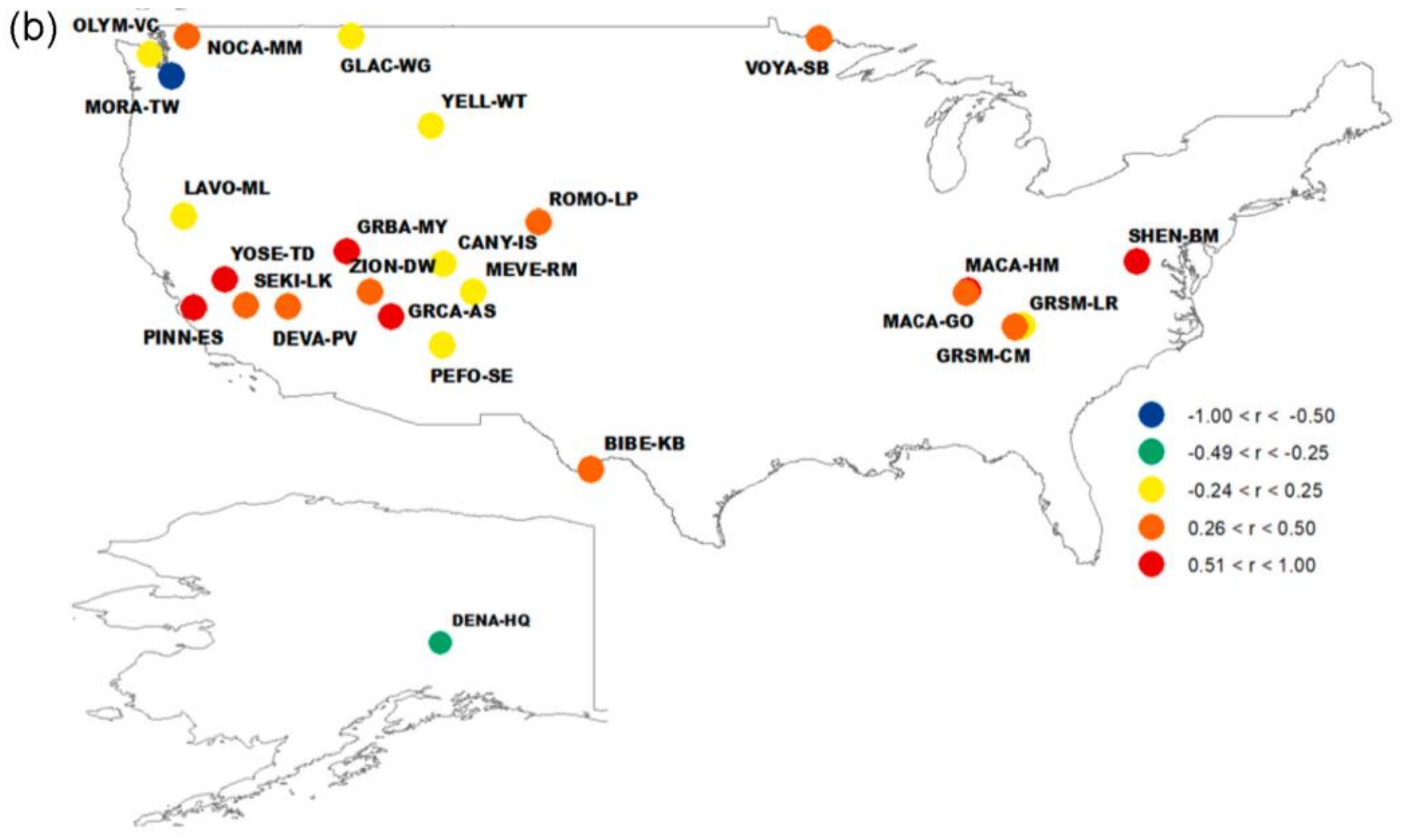
Further, correlation coefficients between component 9 (C9) and component 10 (C10) for temperature and ozone were calculated. Given that both of the components are distributed nonparametrically, correlation coefficients were determined using the Spearman Rank Order Correlation test. Resulting correlation coefficients for each site are shown in Figure 6. Values of significance for correlation coefficients between C9 for temperature and ozone were all within the 95% confidence limit, except for DENA-HQ (p = 0.24) and MACA-GO (p = 0.21). Values of significance for correlation coefficients between the two C10 signals were all within the 95% confidence limit. C9 correlation coefficients (Figure 6a) were strongly correlated (r > 0.5 or r < −0.50) at 4 of 25 sites and were weakly correlated (0.3 < r < 0.5) at 8 of 25 sites. Signal C9 of ozone oscillates on a similar timescale to this component in temperature therefore, it is suggested to represent ENSO. Its significant correlation with that of ozone thus indicated the contribution of ENSO to surface ozone. Signal C10 in temperature and ozone were strongly correlated (r > 0.50 or r < −0.50) at 8 of 25 sites and were weakly correlated (0.30 < r < 0.50 or −0.30 < r < −0.50) at 9 of 25 sites (Figure 6b). Signal C10 for ozone oscillates about every 8–12 years, which is a similar time scale to temperature, and was thus suggested to represent PDO. Its correlation with C10 in ozone hence alludes to the same process driving ozone.
Individually, components C9 and C10, or variability by ENSO and PDO, contribute about 1–2% to the variance in ozone concentrations. However, both of the components have a modulating effect on the seasonal cycle as well as subsequent higher frequency components. The modulation effect of lower frequency signals on higher frequency signals can be illustrated using the seasonal cycle of Rocky Mountain National Park (ROMO-LP). In Figure 7, signals of the seasonal cycle (C7), ENSO (C9), and PDO (C10) for Rocky Mountain National Park (ROMO-LP) are superimposed. Black arrows indicate that ENSO and PDO are out-of-phase, while gray arrows indicate that the components are in-phase. For example, in spring 2003, 2011, and 2012 the seasonal cycle was enhanced by 3–4 ppbv from the previous year, while ENSO and PDO were in phase. Therefore, when ENSO and PDO act in concert and the regimes in these climate modes have reached a peak, maximums in the seasonal cycle were enhanced. Modulation, or the enhancement of the seasonal cycle, by lower frequency components occurs at all sites in the study domain.
4. Discussion
4.1. Impacts of Domestic Emissions Reductions on Rural Ozone Trends
Declining trends were found to be −0.27 to −0.6 ppbv yr−1 in the East and −0.02 to −0.63 ppbv yr−1 in the West (Figure 3b). The most significant trend decreases in the West/ Intermountain West were seen at ZION-DW with decreases at a rate of -0.63 ppbv yr-1. The second most significant decreases in this region were seen at PINN-ES, where decreasing trends (Figure 3b) were observed throughout the monitoring period (Figure 1). This site has some of the earliest ozone measurements in the study domain, beginning in 1987, and is currently still monitoring. The eastern U.S. has the earliest shift in trend status from positive to negative, with sites in central California and the Northwestern U.S. following suit thereafter (Table 2). The first sites in the west to change from positive to negative trends were SEKI-LK (16 April 1997) and YOSE-TD (19 November 1998), which are the closest in proximity to PINN-ES (Table 2; Figure 1). It should be noted that, of the sites with the earliest shift from positive to negative (1995–2003), all of them are located near urban regions, which include central California, Northwestern Washington, and the Eastern U.S., which have experienced more significant decreases in ozone trends relative to rural areas [9]. This trend was found out by Cooper et al. [9] but it should be pointed out that their work did not include sites in the Northwestern U.S. Three sites in this work MORA-TW, NOCA-MM, and OLYM-VC are located in the Northwestern and are in close proximity to the Seattle metropolitan area. The timing of the ozone reductions within the greater Seattle metropolitan area coincides with the findings of Simon et al. [3], which showed that both NOx and VOC emissions decreased by 39.6% and 14%, respectively, in the Northwestern U.S. between 2000 and 2011.
Cooper et al. [9] identified the Denver Metropolitan area as a region that did not have significant reductions in ozone precursor emissions, while they attributed Los Angeles Basin ozone decreases to VOC emission reductions, based on nation-wide emission inventories within the 1980–1995 time period. The U.S. EPA’s State Tier 1 database reported Colorado’s estimated 2000 NOx emissions were reduced by 1762 tons when compared against 1990 levels, decreasing from 33,381 tons to 31,619 tons, for a 5.3% reduction [40]. California’s estimated NOx emissions between 1990 and 2000 were reduced by 16.0%, decreasing from 171,382 tons to 143,936 tons, for a reduction of 27,446 tons [40]. For example, decreasing trends in ozone were not observed until 2009 at ROMO-LP, which is located upwind of the Denver Metropolitan region (Table 2), which coincides with a 15.0% reduction in Colorado’s estimated Tier 1 NOx emissions between 1990 and 2005 [40]. In contrast to Colorado, the Los Angeles Basin, ozone levels decreased by 50 ppbv between 1979 and 1997 (followed by no decreases over 1997–2008), which is potentially the cause of the earlier start of decreasing trends in ozone at two sites upwind of Los Angeles (YOSE-TD and SEKI-LK). PINN-ES has exhibited a decreasing trend in ozone since its inception as an ozone monitoring site, but it is in relatively close proximity to the coast when compared to the other central California sites and is influenced by marine air; therefore, it is less likely to be affected by the Los Angeles Basin, like the other central California sites. In the eastern states of Virginia and Kentucky and the western states of Washington and California, where all of the sites with the earliest of trend reversals are located (prior to 2003), the State Tier 1 NOx emission reductions between 1990 and 2000 were −12.0% in VA, −10.5% in KY, −14.3% in WA, and −16.0% in CA [40]. The earliest emission reductions in the Intermountain West occurred in the Denver Metropolitan area of Colorado in 1997. However, many states in the Intermountain West have seen a significant shift in source sectors, in addition to increases in frequency and magnitude of wildfires [41,42,43,44], all of which may be influencing the increasing ozone trends that were observed at BIBE-KB and GLAC-WG.
4.2. Variability in the Seasonal Cycle of U.S. Surface Ozone
Parrish et al. [18] suggested several hypotheses to explain the shift in the seasonal cycle which include changes in emissions and ozone photochemistry, variability in transport pathways, and climate factors. Emission reductions have likely impacted the trends in ozone at sites nearest large urban areas, which could have also affected the annual amplitude and the shift in seasonal cycles. Rising springtime ozone of ~0.6 ppbv year−1 in the western U.S. from 1984 to 2008 was identified by Cooper et al. [24,26], and was thought to result from the changing distribution of ozone precursors; this subsequently caused the shift in seasonal cycles and decreased annual amplitude [26]. Specifically, decreased NOx emissions could have decreased annual ozone peaks, but it also reduced ozone removal via NO titration [25], the latter of which has led to increased wintertime and early springtime ozone levels [4,9,18,45]. Hence, increased springtime ozone and decreased summertime ozone may be a key driver of the shift in the ozone annual peak to earlier in the year [26].
There was greater regional continuity in the East than the West, with four out of six sites showing significant decreases in the magnitude of annual amplitude (Figure 4b), four out of six sites with a significant shift in annual maximum (Figure 5b), and three out of six sites with a significant shift in annual minimum (Figure 5d). In comparison, 5 out of 19 west coastal sites have had changes in the magnitude of annual peaks and minimums. Of the sites in the West, three out of four sites had significant decreases in annual amplitude. Three out of five, and four out of five sites for annual maximum and minimum, respectively, were located in the regions with the earliest shift in trends from positive to negative (Figure 5a,c). Parrish et al. [18] suggested that the shift in the seasonal cycle may be a phenomenon occurring across northern mid-latitudes. Our study suggests that this shift did not seem to occur uniformly at all mid-latitudinal locations, as overall across the U.S. 9/25 (8/25), NPS sites have had a change in timing of annual maximums (minimums), and 11/25 have had a change in annual amplitude.
4.3. Effects of Large-Scale Climate Circulation on Seasonal Cycles of U.S. Surface Ozone
Studies have suggested that various modes of climate variability and related dynamical mechanisms are responsible for the changes in free tropospheric and surface ozone [6,8,39,46,47,48]. Lin et al. [6,8,48] investigated the impact of large-scale climate perturbations on U.S. surface ozone trends using a global chemistry climate model, and their results show that they have a clear impact on the seasonal variability in ozone. For instance, the positive PDO over 1977–1998 was accompanied by stronger and more prolonged El Niño events, followed by a negative PDO between 1999 and 2015 with stronger and more prolonged La Niña events [8]. This has implications for the transport of East Asian pollution and subsequently the seasonal cycle of U.S. surface ozone.
The dynamics of PDO and ENSO could explain the modulatory effect of ENSO and PDO on the seasonal cycle of ozone at the majority of the NPS sites, as shown in Section 3.3. In the positive phase of ENSO and PDO, zonal winds in winter are heightened [8,38,49]. This manifests as an increase in transpacific transport of Asian pollution to the southwestern U.S. via a strengthened subtropical jet stream in late winter and early spring [10,50], likely leading to springtime ozone and perhaps higher annual maximum ozone there. During La Niña and negative PDO periods, the northward shifting subtropical jet stream directs East Asian pollution to the Pacific Northwest [6,51], likely increasing the surface ozone levels in Alaska and the northwestern U.S., whereas in other parts of the U.S. surface ozone was lowered. The long term increasing trend in surface ozone in Alaska was to be discussed further in Section 4.4. In addition to variability in transport, El Niño episodes bring warm and dry conditions to the central and southern part of the country, ripe conditions for ozone formation [38], whereas La Niña episodes bring increased storms and cloudiness as well as cooler temperatures; therefore, ozone formation is not as strong during La Niña periods [38]. This also seems consistent with the modulatory effect of ENSO/PDO on the seasonal cycle.
4.4. Increasing Annual 4th-Highest DM8HA and Annual Amplitude of Ozone at DENA-HQ over 1987–2015
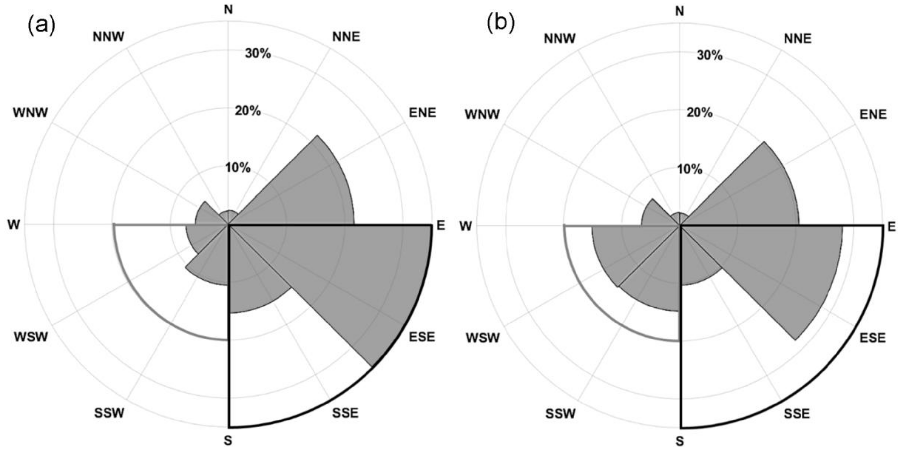
Denali National Park (DENA-HQ) (63.7258° N, 148.9633° W) is the only location where an increase in annual amplitude was found throughout the monitoring period. The annual maximum DM8HA value increased by 2 ppbv between 1987 and 2015 (Figure 4c), while the annual minimum value decreased by 2 ppbv (Figure 5a). In addition to this, there has been a statically significant increase in the annual 4th-highest DM8HA. The annual 4th-highest DM8HA is found to be increasing at a rate of 0.33 ppbv year−1 (R2 = 0.29, p < 0.05) (a total increase of ~9 ppbv) (Figure 8). The annual 4th-highest DM8HA does not occur during DENA-HQ’s peak ozone season of late March to early April, but rather late April to May. This is likely due to the influence of higher solar irradiance coupled with transpacific transport [52]. It is important to note that the overall multidecadal trend at this site has not changed. However, the increasing trend in the annual 4th-highest DM8HA coupled with the increase in annual peak ozone values could signal the beginning of a multidecadal ozone trend increase at DENA-HQ in the future. As aforementioned, the persistence of the negative PDO since 1998–1999, concurrent with more La Niña events, has resulted in a shift in transport of East Asian pollution to higher latitudes (45°–50°), which has subsequently increased the number of polluted air masses that are arriving to this region. To demonstrate the influence of polluted air masses that are transported from East Asia to DENA-HQ, back trajectories were conducted for the seven days before and after the date of the annual 4th highest DM8HA value occurrence at 22:00 UTC (14:00 Alaskan time), the average 8-h rolling average start time for two time periods, 1987–1998 and 1999–2015. Of the 29 DM8HA values for the DENA-HQ record, 27 of them occurred in the months of April or May. Seven day back trajectories were calculated from DENA-HQ during these months, following the works of Jaffe et al. [53], Berntsen et al. [54], Yienger et al. [55,56], and Holzer et al. [57], which found that the average transport time in the spring between North America and Asia was ~7 days. These trajectories were plotted and the area around the arrival point (DENA-HQ) was divided into eight sectors of 45° (Figure 9).
Over 1987–1998, 72% of trajectories were from the area East-North-East to South (ENE–S) of DENA-HQ (Figure 9), which suggests that the majority of air masses that are arriving at the site originated from the marine boundary layer and western Canada. Over 1999–2015, 13% more trajectories came from West to South (W–S) of DENA-HQ, while 12% less from the east-south directions when compared to the 1987–1998 period. This means that during the time period from 1999 to 2015, air mass transport was more frequent from the North Pacific, with an increased potential of transporting East Asian pollution to DENA-HQ, and less frequently from above the Arctic Circle over land and near coastal regions of Canada, where the air is mostly pristine.
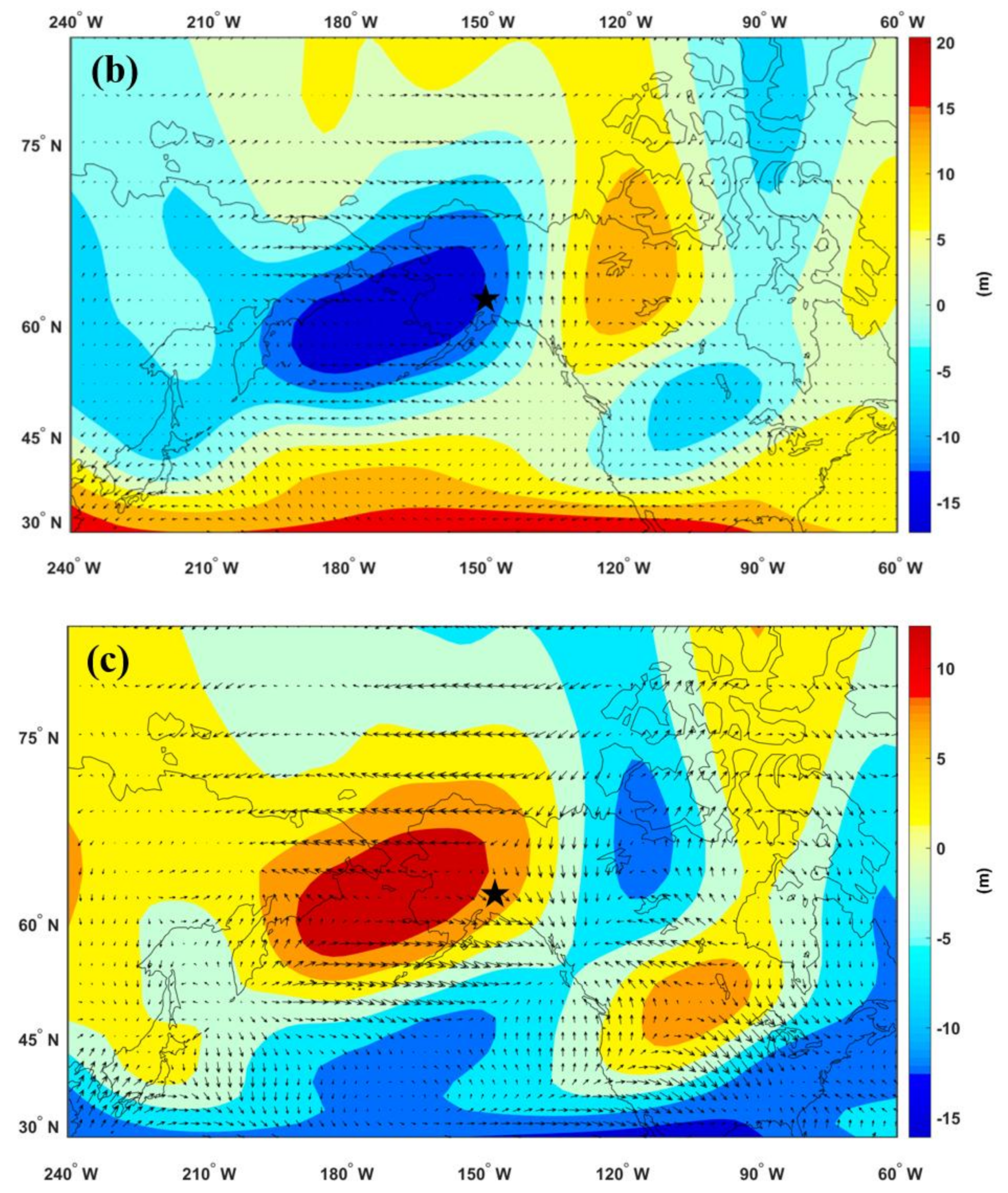
To determine the key factors driving the variability in the direction of backward trajectories between the two periods (1987–1998 and 1999–2015) for the months of April and May, monthly mean geopotential height fields with wind speeds at 500 hPa for 1987–2015, 1987–1998 (period one), and 1998–2015 (period two) were examined for April and May during each period (Figure 10). Anomalously low geopotential heights occurred to the west of Alaska for period one (Figure 10b); during period two, anomalously high geopotential heights occurred in the same area (Figure 10c). These findings are in agreement with Bond and Harrison’s [58] study on the variability and relationship between ENSO and the Arctic Oscillation on the climate of Alaska, but for the winter months of November through February. The increased number of El Niño events that occurred during the positive PDO phase over 1987–1998 resulted in a low-pressure system to the southwest of Alaska during April and May, the months when transport over the Pacific is the greatest [57], allowing for air masses to preferentially move from the U.S. West Coast and the marine regions south of Alaska. During the second period 1999–2015 in the months of April and May, a high-pressure system resulted in increased westerly flow across the North Pacific to DENA-HQ and a decrease in the air masses from the marine regions south of Alaska. Air masses originating from this region for the week before and after a peak ozone event in at DENA-HQ are presumably more polluted. It is likely that there was pollution outflow during these times from East Asia, causing the increase in ozone at this site. Therefore, the changing circulation regimes enhanced the transport of western polluted air masses to Alaska during period two, ultimately leading to the increasing trends in the annual 4th highest DM8HA values and the magnitude of the annual amplitude after 1999 at DENA-HQ.
5. Conclusions
In this study, 25 U.S. NPS datasets were analyzed for spatial and temporal variability in long-term ozone using EEMD. This method has allowed for an analysis of the spatial and temporal variability of long-term ozone data on four time-scales, which include annual, interannual, interdecadal, and multidecadal. Peak values in the ozone seasonal component have shifted to earlier in the year at nine sites by 10–60 days, while minimum values have shifted to earlier in the year at eight sites by 14–34 days. There has been a decrease in annual maximum values and an increase in annual minimum values at eight sites by 5–20 ppbv year−1. The changes that were seen in the seasonal cycle were likely the result of decreasing NOx concentrations that would result in a change in the distribution of ozone throughout the year, leading to an increase in minimum ozone values and a decrease in maximum ozone values. Interannual and interdecadal cycles resulting from ENSO and PDO have a constant effect on higher frequency components. This effect was examined using the seasonal component where we found the greatest enhancement in ozone concentrations of 3–4 ppbv in the annual maximum value when ENSO and PDO were both positive and in-phase. Multidecadal trends were identified to change from increasing to decreasing at 20 of the 25 sites. Increasing trends were found to be between 0.001 ppbv and 0.4 ppbv year−1, while decreasing trends were found to be between −0.02 to −0.63 ppbv year−1. The multidecadal trend shifted from positive to negative prior to 2004 at sites in the eastern U.S., Southern California, and the Pacific Northwest. In the Intermountain West, trends shifted from positive to negative most predominately after 2004. Decades of increasing annual amplitude, annual 4th highest DM8HA, as well as a shift in date for both of these variables at Denali National Park in Alaska (DENA-HQ) may have resulted from a change in transport pathways related to the PDO. These changes likely stemmed from an increase in the strength and longevity of La Niña events over 1999–2015, and a negative PDO period, which increased the transport of heavily polluted air masses from East Asia by 13% from the previous PDO period of 1987–1998.
The findings from this study can be used to aid in future ozone mitigation strategies and policies in the United States. The modulatory effects of large circulation processes on higher frequency components can be useful in predicting high ozone events in the U.S. A more extensive analysis incorporating more sites across the U.S. and other components of the ozone data sets are warranted to better understand and assess the impact of major climate modes on U.S. ozone trends and variability.
Acknowledgments
This work was in part supported by National Park Service. We gratefully acknowledge the assistance of Jessica Ward, Air Resources Specialists, Inc. for retrieving and providing the National Park Service data. Additional data were acquired from the European Center for Medium Range Data and have made this work possible. This paper has not been subjected to EPA peer and administrative review; therefore, the conclusions and opinions contained herein are solely those of the authors and should not be construed to reflect the views of the EPA. The assumptions, findings, conclusions, judgments, and views presented herein are those of the authors and should not be interpreted as necessarily representing the NPS.
Author Contributions
Deborah F. McGlynn performed all data analysis and wrote the majority of the manuscript. Huiting Mao contributed significant scientific insight and direction as well as writing and editing of the manuscript. Zhaohua Wu provided the EEMD code as well as valuable insight into data processing and meaning of results. Barkley Sive helped with data collection, editing and interpretation of some results. Timothy Sharac assisted with editing and writing of a portion of the manuscript.
Conflicts of Interest
The authors declare no conflict of interest.
References
- US Environmental Protection Agency. National Ambient Air Quality Standard for Ozone; Final Rule-2015; US Environmental Protection Agency: Washington, DC, USA, 2015; Volume 80.
- US Environmental Protection Agency. National Ambient Air Quality Standards for Ozone; Final Rule-2008; US Environmental Protection Agency: Washington, DC, USA, 2008; Volume 73.
- Simon, H.; Reff, A.; Wells, B.; Xing, J.; Frank, N. Ozone trends across the United States over a period of decreasing NOx and VOC emissions. Environ. Sci. Technol. 2015, 49, 186–195. [Google Scholar] [CrossRef] [PubMed]
- Parrish, D.D.; Law, K.S.; Staehelin, J.; Derwent, R.; Cooper, O.R.; Tanimoto, H.; Volz-Thomas, A.; Gilge, S.; Scheel, H.-E.; Steinbacher, M.; et al. Long-term changes in lower tropospheric baseline ozone concentrations at northern mid-latitudes. Atmos. Chem. Phys. 2012, 12, 11485–11504. [Google Scholar] [CrossRef] [Green Version]
- Jacob, D.J.; Logan, J.A.; Murti, P.P. Effect of rising Asian emissions on surface ozone in the United States. Geophys. Res. Lett. 1999, 26, 2175–2178. [Google Scholar] [CrossRef]
- Lin, M.; Fiore, A.M.; Horowitz, L.W.; Langford, A.O.; Oltmans, S.J.; Tarasick, D.; Rieder, H.E. Climate variability modulates western US ozone air quality in spring via deep stratospheric intrusions. Nat. Commun. 2015, 6, 7105–7116. [Google Scholar] [CrossRef] [PubMed]
- Lin, M.; Horowitz, L.W.; Payton, R.; Fiore, A.M.; Tonnesen, G. US surface ozone trends and extremes from 1980 to 2014: Quantifying the roles of rising Asian emissions, domestic controls, wildfires, and climate. Atmos. Chem. Phys. 2017, 17, 2943–2970. [Google Scholar] [CrossRef]
- Lin, M.; Horowitz, L.W.; Oltmans, S.J.; Fiore, A.M.; Fan, S. Tropospheric ozone trends at Mauna Loa Observatory tied to decadal climate variability. Nat. Geosci. 2014, 7, 136–143. [Google Scholar] [CrossRef]
- Cooper, O.R.; Gao, R.S.; Tarasick, D.; Leblanc, T.; Sweeney, C. Long-term ozone trends at rural ozone monitoring sites across the United States, 1990–2010. J. Geophys. Res. Atmos. 2012, 117, D22307. [Google Scholar] [CrossRef]
- Oman, L.D.; Ziemke, J.R.; Douglass, A.R.; Waugh, D.W.; Lang, C.; Rodriguez, J.M.; Nielsen, J.E. The response of tropical tropospheric ozone to ENSO. Geophys. Res. Lett. 2011, 38, L13706. [Google Scholar] [CrossRef]
- Fiore, A.M.; Naik, V.; Leibensperger, E.M. Air Quality and Climate Connections. J. Air Waste Manage. Assoc. 2015, 65, 645–685. [Google Scholar] [CrossRef] [PubMed]
- Parrish, D.D.; Petropavlovskikh, I.; Oltmans, S.J. Reversal of Long-Term Trend in Baseline Ozone Concentrations at the North American West Coast. Geophys. Res. Lett. 2017, 44, 10675–10681. [Google Scholar] [CrossRef]
- Zhang, L.; Jacob, D.J.; Boersma, K.F.; Jaffe, D.A.; Olson, J.R.; Bowman, K.W.; Worden, J.R.; Thompson, A.M.; Avery, M.A.; Cohen, R.C.; et al. Transpacific transport of ozone pollution and the effect of recent Asian emission increases on air quality in North America: An integrated analysis using satellite, aircraft, ozonesonde, and surface observations. Atmos. Chem. Phys. Discuss. 2008, 8, 8143–8191. [Google Scholar] [CrossRef]
- Lin, M.; Fiore, A.M.; Horowitz, L.W.; Cooper, O.R.; Naik, V.; Holloway, J.; Johnson, B.J.; Middlebrook, A.M.; Oltmans, S.J.; Pollack, I.B.; et al. Transport of Asian ozone pollution into surface air over the western United States in Spring. J. Geophys. Res. Atmos. 2012, 117, D00V07. [Google Scholar] [CrossRef]
- Ziemke, J.R. La Niña and El Niño—Induced variabilities of ozone in the tropical lower atmosphere during 1970–2001. Geophys. Res. Lett. 2003, 30, 1142. [Google Scholar] [CrossRef]
- Langford, A.O.; Masterst, C.D. Modulation of Middle and upper tropospheric ozone at Northern midlatitudes by the El Niño Southern Oscillation. J. Geophys. Res. 1998, 25, 2667–2670. [Google Scholar] [CrossRef]
- Koumoutsaris, S.; Bey, I.; Generoso, S.; Thouret, V. Influence of El Niño-Southern Oscillation on the interannual variability of tropospheric ozone in the northern midlatitudes. J. Geophys. Res. Atmos. 2008, 113, D19301. [Google Scholar] [CrossRef]
- Parrish, D.D.; Law, K.S.; Staehelin, J.; Derwent, R.; Cooper, O.R.; Tanimoto, H.; Volz-Thomas, A.; Gilge, S.; Scheel, H.-E.; Steinbacher, M.; et al. Lower tropospheric ozone at northern midlatitudes: Changing seasonal cycle. Geophys. Res. Lett. 2013, 40, 1631–1636. [Google Scholar] [CrossRef]
- Carslaw, D.C. On the changing seasonal cycles and trends of ozone at Mace Head, Ireland. Atmos. Chem. Phys. Discuss. 2005, 5, 5987–6011. [Google Scholar] [CrossRef]
- Bloomer, B.J.; Vinnikov, K.Y.; Dickerson, R.R. Changes in seasonal and diurnal cycles of ozone and temperature in the eastern U.S. Atmos. Environ. 2010, 44, 2543–2551. [Google Scholar] [CrossRef]
- Monks, P.S. A review of the observations and origins of the spring ozone maximum. Atmos. Environ. 2000, 34, 3545–3561. [Google Scholar] [CrossRef]
- Wang, Y. Springtime photochemistry at northern mid and high latitudes. J. Geophys. Res. 2003, 108, 8358–8390. [Google Scholar] [CrossRef]
- Salisbury, G.; Monks, P.S.; Bauguitte, S.; Bandy, B.J.; Penkett, S.A. A Seasonal Comparison of the Ozone Photochemistry in Clean and Polluted Air Masses at Mace Head, Ireland. J. Atmos. Chem. 2002, 41, 163–187. [Google Scholar] [CrossRef]
- Cooper, O.R.; Parrish, D.D.; Stohl, A.; Trainer, M.; Nédélec, P.; Thouret, V.; Cammas, J.P.; Oltmans, S.J.; Johnson, B.J.; Tarasick, D.; et al. Increasing springtime ozone mixing ratios in the free troposphere over western North America. Nature 2010, 463, 344–348. [Google Scholar] [CrossRef] [PubMed]
- Jonson, J.E.; Simpson, D.; Fagerli, H.; Solberg, S. Can we explain the trends in European ozone levels? Atmos. Chem. Phys. 2006, 6, 51–66. [Google Scholar] [CrossRef]
- Cooper, O.R.; Parrish, D.D.; Ziemke, J.; Balashov, N.V.; Cupeiro, M.; Galbally, I.E.; Gilge, S.; Horowitz, L.; Jensen, N.R.; Lamarque, J.-F.; et al. Global distribution and trends of tropospheric ozone: An observation-based review. Elem. Sci. Anthr. 2014, 2. [Google Scholar] [CrossRef]
- Wu, Z.; Huang, N.E. Ensemble Empirical Mode Decomposition: A Noise Assisted Data Analysis Method. Adv. Adapt. Data Anal. 2009, 1, 385–388. [Google Scholar] [CrossRef]
- NPS Gaseous Pollutant and Met Data. Available online: https://ard-request.air-resource.com/ (accessed on 5 February 2018).
- National Park Service, Air Resources Division. Gaseous Pollutant Monitoring Program Quality Assurance Project Plan (QAPP); National Park Service, U.S. Department of the Interior: Denver, CO, USA, 2015.
- Wu, Z.; Huang, N.E.; Long, S.R.; Peng, C.-K. On the trend, detrending, and variability of nonlinear and nonstationary time series. Proc. Natl. Acad. Sci. USA 2007, 104, 14889–14894. [Google Scholar] [CrossRef] [PubMed]
- McDonald-Buller, E.C.; Allen, D.T.; Brown, N.; Jacob, D.J.; Jaffe, D.; Kolb, C.E.; Lefohn, A.S.; Oltmans, S.; Parrish, D.D.; Yarwood, G.; et al. Establishing Policy Relevant Background (PRB) Ozone Concentrations in the United States. Environ. Sci. Technol. 2011, 45, 9484–9497. [Google Scholar] [CrossRef] [PubMed]
- ECMWF. Advancing global NWP through international collaboration. Available online: https://www.ecmwf.int/ (accessed on 5 February 2018).
- Draxler, R.; Stunder, B.; Rolph, G.; Stein, A.; Taylor, A. HYSPLIT4 User’s Guide; NOAA Air Resources Laboratory: Silver Spring, MD, USA, 2016.
- Derwent, R.G.; Jenkin, M.E.; Saunders, S.M.; Pilling, M.J. Photochemical ozone creation potentials for organic compounds in northwest Europe calculated with a master chemical mechanism. Atmos. Environ. 1998, 32, 2429–2441. [Google Scholar] [CrossRef]
- Papineau, J.M. Wintertime temperature anomalies in Alaska correlated with ENSO and PDO. Int. J. Climatol. 2001, 21, 1577–1592. [Google Scholar] [CrossRef]
- Zhang, A.; Jia, G.; Epstein, H.E.; Xia, J. ENSO elicits opposing responses of semi-arid vegetation between Hemispheres. Sci. Rep. 2017, 7, 42281–42290. [Google Scholar] [CrossRef] [PubMed]
- Stuecker, M.F.; Timmermann, A.; Jin, F.-F.; McGregor, S.; Ren, H.-L. A combination mode of the annual cycle and the El Niño/Southern Oscillation. Nat. Geosci. 2013, 6, 540–544. [Google Scholar] [CrossRef]
- Newman, M.; Compo, G.P.; Alexander, M.A. ENSO-Forced Variability of the Pacific Decadal Oscillation. J. Clim. 2003, 16, 3853–3857. [Google Scholar] [CrossRef]
- Timmermann, A.; Latif, M.; Grötzner, A.; Voss, R. Modes of climate variability as simulated by a coupled general circulation model. Part I: ENSO-like climate variability and its low-frequency modulation. Clim. Dyn. 1999, 15, 605–618. [Google Scholar] [CrossRef]
- US Environmental Protection Agency. Air Pollutant Emissions Trends Data. Available online: https://www.epa.gov/air-emissions-inventories/air-pollutant-emissions-trends-data (accessed on 19 March 2018).
- Liu, Y.; Goodrick, S.; Heilman, W. Wildland fire emissions, carbon, and climate: Wildfire–climate interactions. For. Ecol. Manage. 2014, 317, 80–96. [Google Scholar] [CrossRef]
- Abatzoglou, J.T.; Williams, A.P. Impact of anthropogenic climate change on wildfire across western US forests. Proc. Natl. Acad. Sci. USA 2016, 113, 11770–11775. [Google Scholar] [CrossRef] [PubMed]
- Liu, J.C.; Mickley, L.J.; Sulprizio, M.P.; Dominici, F.; Yue, X.; Ebisu, K.; Anderson, G.B.; Khan, R.F.A.; Bravo, M.A.; Bell, M.L. Particulate air pollution from wildfires in the Western US under climate change. Clim. Change 2016, 138, 655–666. [Google Scholar] [CrossRef] [PubMed]
- Barbero, R.; Abatzoglou, J.T.; Larkin, N.K.; Kolden, C.A.; Stocks, B. Climate change presents increased potential for very large fires in the contiguous United States. Int. J. Wildl. Fire 2015, 24, 892–899. [Google Scholar] [CrossRef]
- Wilson, R.C.; Fleming, Z.L.; Monks, P.S.; Clain, G.; Henne, S.; Konovalov, I.B.; Szopa, S.; Menut, L. Have primary emission reduction measures reduced ozone across Europe? An analysis of European rural background ozone trends 1996–2005. Atmos. Chem. Phys. 2012, 12, 437–454. [Google Scholar] [CrossRef] [Green Version]
- Rodionov, S.N.; Bond, N.A.; Overland, J.E. The Aleutian Low, storm tracks, and winter climate variability in the Bering Sea. Deep Sea Res. Part II Top. Stud. Oceanogr. 2007, 54, 2560–2577. [Google Scholar] [CrossRef]
- Wilcox, L.J.; Highwood, E.J.; Dunstone, N.J. The influence of anthropogenic aerosol on multi-decadal variations of historical global climate. Environ. Res. Lett. 2013, 8, 24033–24042. [Google Scholar] [CrossRef]
- Lin, M.; Fiore, A.M.; Cooper, O.R.; Horowitz, L.W.; Langford, A.O.; Levy, H.; Johnson, B.J.; Naik, V.; Oltmans, S.J.; Senff, C.J. Springtime high surface ozone events over the western United States: Quantifying the role of stratospheric intrusions. J. Geophys. Res. Atmos. 2012, 117, D00V22. [Google Scholar] [CrossRef]
- L’Heureux, M.L. Atmospheric circulation influences on seasonal precipitation patterns in Alaska during the latter 20th century. J. Geophys. Res. 2004, 109, D06106. [Google Scholar] [CrossRef]
- Stein, K.; Timmermann, A.; Schneider, N.; Jin, F.F.; Stuecker, M.F. ENSO seasonal synchronization theory. J. Clim. 2014, 27, 5285–5310. [Google Scholar] [CrossRef]
- NOAA. ESRL Physical Sciences Division Pacific Decadal Oscillation Index. Available online: https://www.esrl.noaa.gov/psd/gcos_wgsp/Timeseries/PDO/ (accessed on 5 September 2017).
- Dentener, F.; Keating, T.; Akimoto, H. Hemispheric Transport of 2010 Part A: Ozone and Particulate Matter; United Nations Publication: Geneva, Switzerland, 2010; ISBN 978-92-1-117043-6. [Google Scholar]
- Jaffe, D.; Anderson, T.; Covert, D.; Kotchenruther, R.; Trost, B.; Danielson, J.; Simpson, W.; Berntsen, T.; Karlsdottir, S.; Blake, D.; et al. Transport of Asian air pollution to North America. Geophys. Res. Lett. 1999, 26, 711–714. [Google Scholar] [CrossRef]
- Berntsen, T.K.; Karlsdóttir, S.; Jaffe, D.A. Influence of Asian emissions on the composition of air reaching the north western United States. Geophys. Res. Lett. 1999, 26, 2171–2174. [Google Scholar] [CrossRef]
- Yienger, J.J.; Galanter, M.; Holloway, T.A.; Phadnis, M.J.; Guttikunda, S.K.; Carmichael, G.R.; Moxim, W.J.; Levy, H. The episodic nature of air pollution transport from Asia to North America. J. Geophys. Res. Atmos. 2000, 105, 26931–26945. [Google Scholar] [CrossRef]
- Yienger, J.; Carmichael, G.; Phadnis, M.; Guttikunda, S.; Holloway, T.; Galanter, M.; Moxim, W.; Levy, H., II. Transport of Air Pollution From Asia To North America. Air Pollut. Model. Its Appl. XIV 2001, 307–313. [Google Scholar]
- Holzer, M.; Hall, T.M.; Stull, R.B. Seasonality and weather-driven variability of transpacific transport. J. Geophys. Res. 2005, 110, D23103. [Google Scholar] [CrossRef]
- Bond, N.A.; Harrison, D.E. ENSO’s effect on Alaska during opposite phases of the Arctic Oscillation. Int. J. Climatol. 2006, 26, 1821–1841. [Google Scholar] [CrossRef]
Figure 1.
Locations of the 25 U.S. National Park Service sites used in this study.

Figure 2.
The four components (ppbv) of interest, C7, C9, C10, and Rn shown here for one site, Rocky Mountain National Park (ROMO-LP). Data capture at this site began in January 1987, but because of a data completeness requirement for EEMD, the start year for this site begins in 1998.
Figure 2.
The four components (ppbv) of interest, C7, C9, C10, and Rn shown here for one site, Rocky Mountain National Park (ROMO-LP). Data capture at this site began in January 1987, but because of a data completeness requirement for EEMD, the start year for this site begins in 1998.
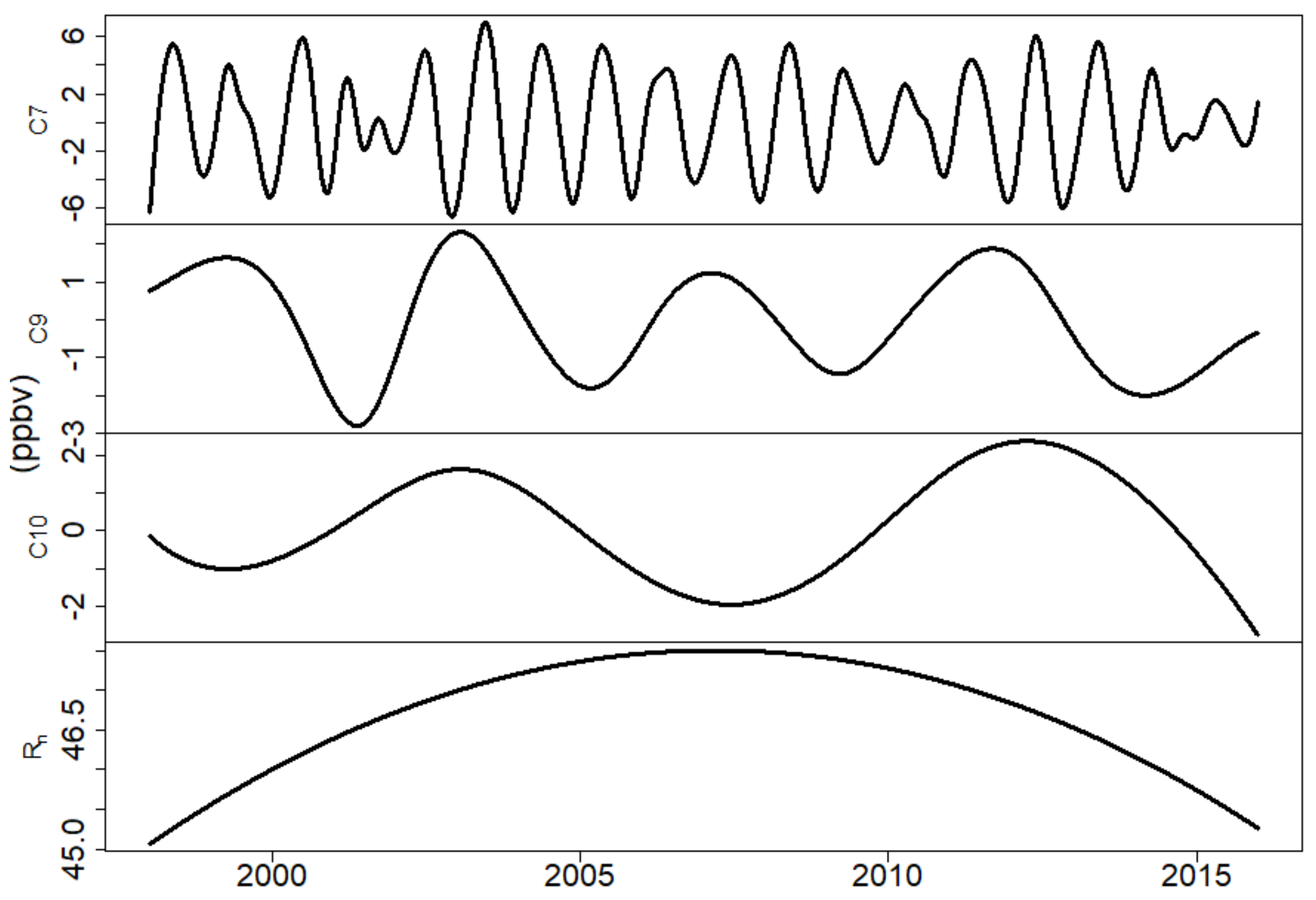
Figure 3.
Increasing (a) and decreasing (b) trends in ppbv yr−1 for all of the sites in the study. The date of trend changes from positive to negative are symbolized for each site. Sites that changed prior to 31 December 2003 are symbolized by triangles and sites that changed after 1 January 2004 are symbolized by squares.

Figure 4.
Sites with a significant negative change in annual amplitude for western (a) and eastern sites (b) and a significant positive change in annual amplitude (c).
Figure 4.
Sites with a significant negative change in annual amplitude for western (a) and eastern sites (b) and a significant positive change in annual amplitude (c).
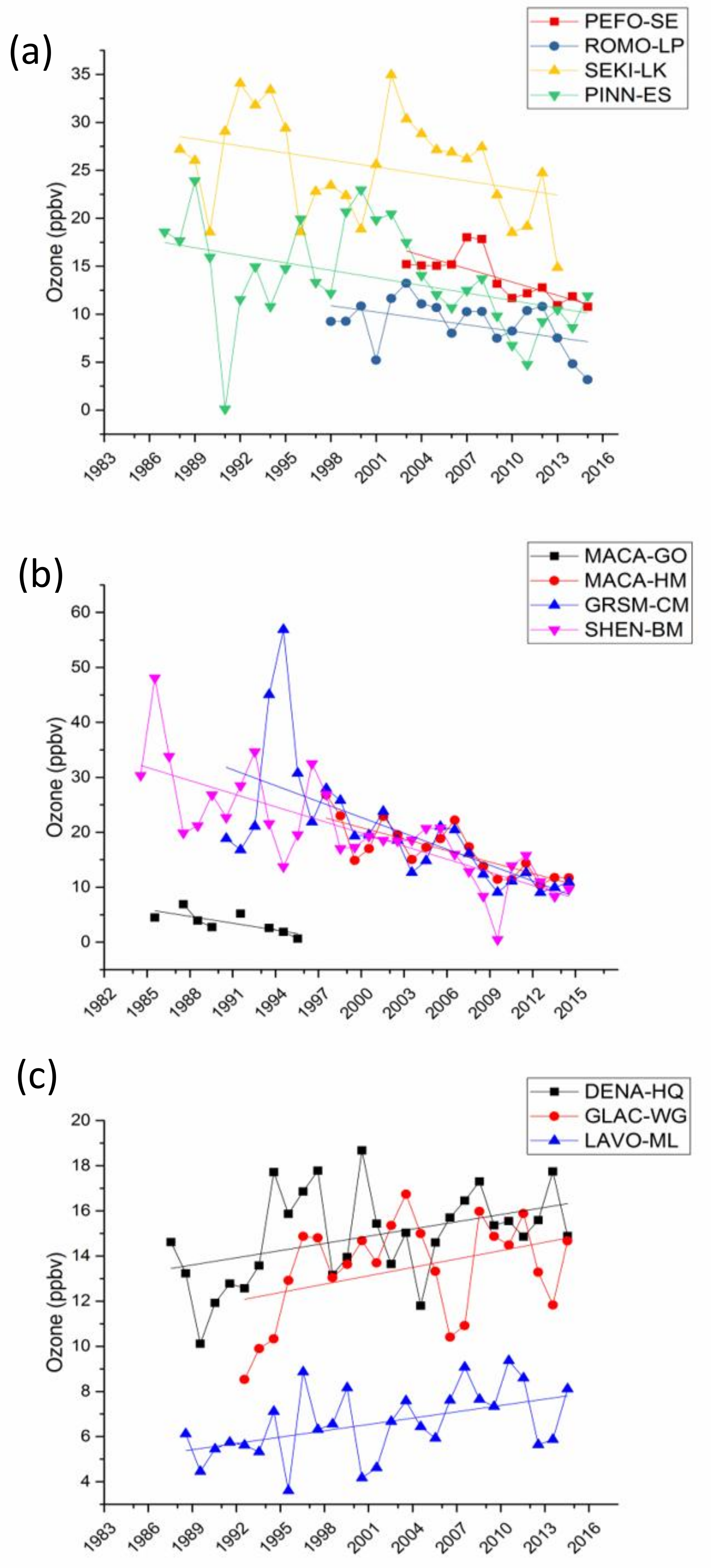
Figure 5.
Significant shifts in the date of annual ozone peak values for the western (a) and eastern (b) sites. Significant shifts in the date of annual ozone minimum values for western (c) and eastern sites (d).
Figure 5.
Significant shifts in the date of annual ozone peak values for the western (a) and eastern (b) sites. Significant shifts in the date of annual ozone minimum values for western (c) and eastern sites (d).

Figure 6.
Spearman rank correlation coefficients between the C9 components for ozone and temperature (a), and the C10 components for ozone and temperature (b).
Figure 6.
Spearman rank correlation coefficients between the C9 components for ozone and temperature (a), and the C10 components for ozone and temperature (b).


Figure 7.
The various effects of C9 and C10 on C7, the seasonal component, depending on the cycle phase. Black arrows indicate that C9 and C10 are out-of-phase; grey arrows indicate that the components are in-phase.
Figure 7.
The various effects of C9 and C10 on C7, the seasonal component, depending on the cycle phase. Black arrows indicate that C9 and C10 are out-of-phase; grey arrows indicate that the components are in-phase.
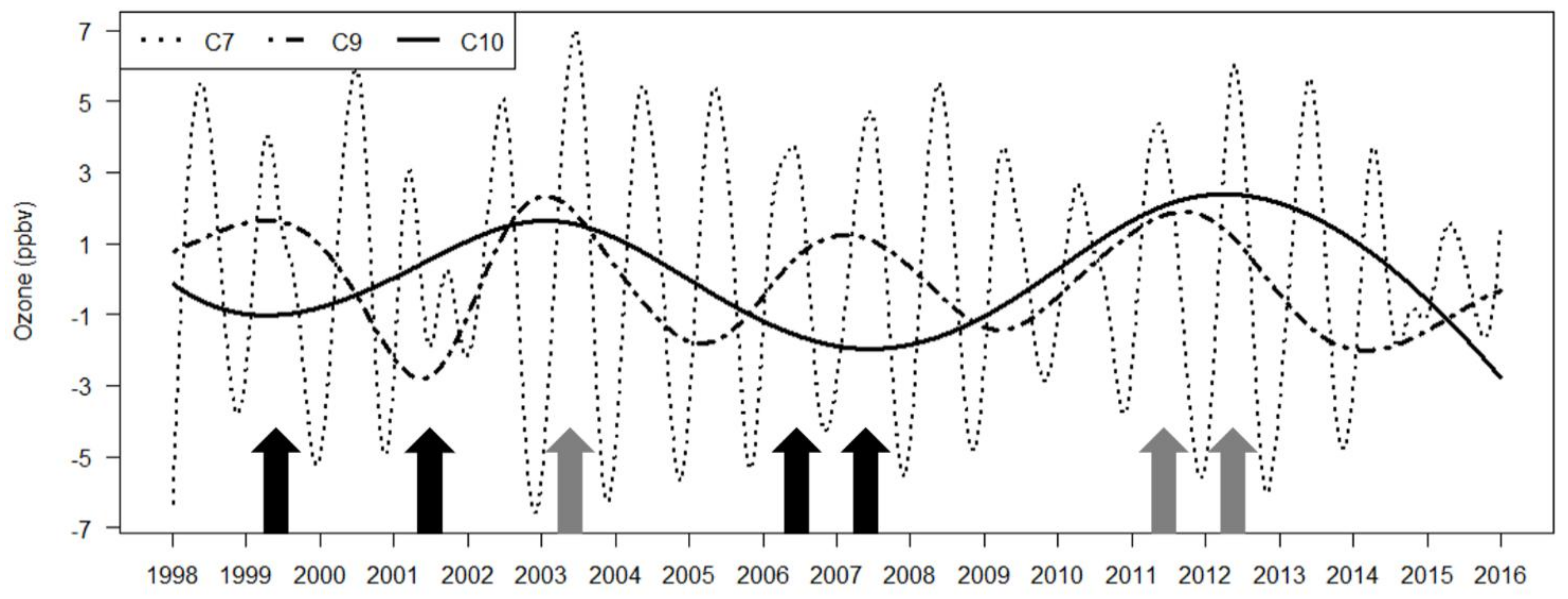
Figure 8.
The annual 4th highest DM8HA at Denali National Park in Alaska (DENA-HQ) and a best fit linear regression line showing a coefficient of determination of 0.29.
Figure 8.
The annual 4th highest DM8HA at Denali National Park in Alaska (DENA-HQ) and a best fit linear regression line showing a coefficient of determination of 0.29.
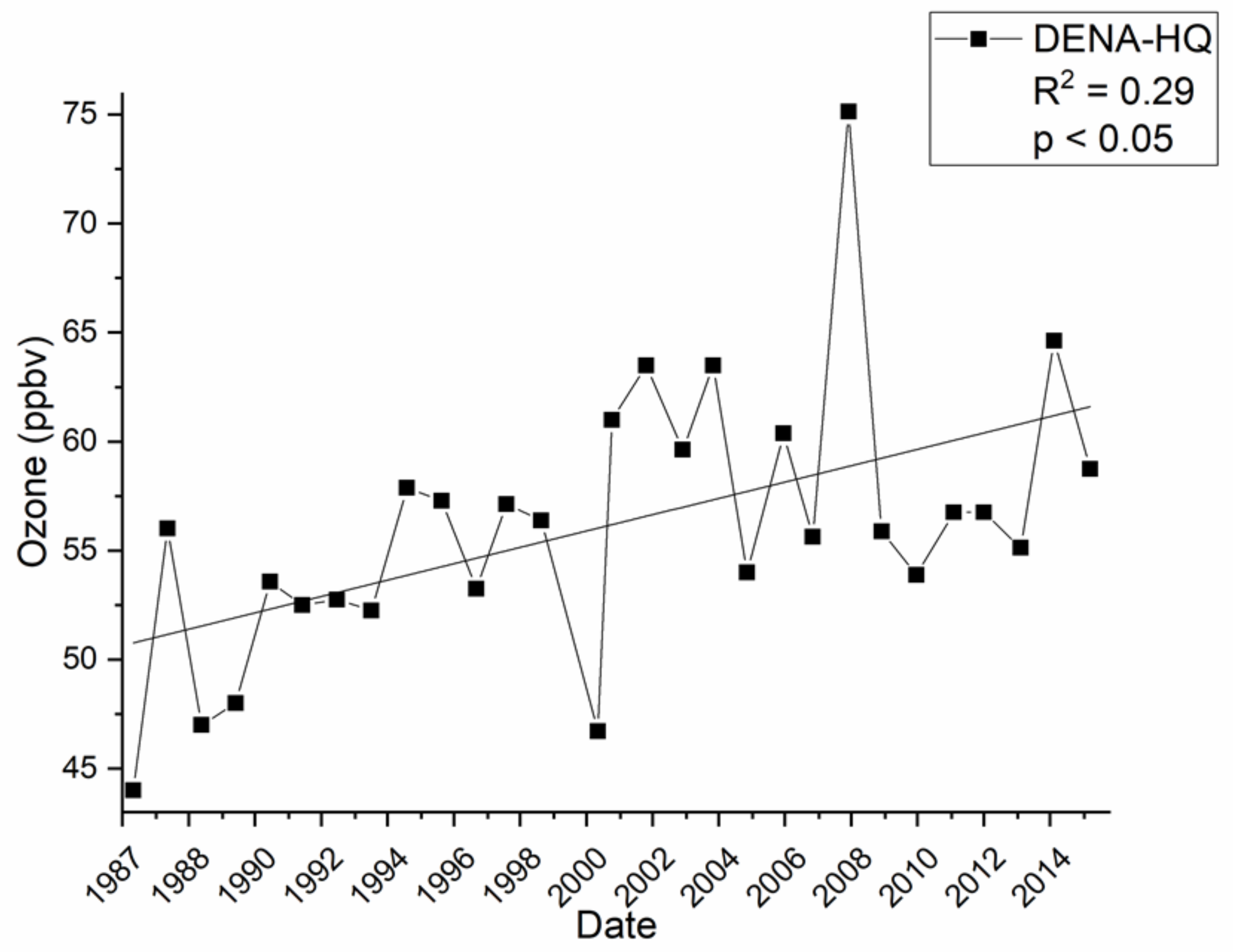
Figure 9.
The percent of trajectories that fell in 8 radial sections around DENA-HQ. Rolling seven-day back trajectories were calculated using the Hybrid Single Particle Lagrangian Integrated model (HYSPLIT) model. Trajectories were calculated seven days before and after the date of the annual 4th-highest DM8HA at DENA-HQ for the periods 1987–1998 (a) and 1999–2015 (b). The grey boxes indicate the area where an increase in trajectories were seen from period one (a) to period two (b) and the black box indicates where a decrease in trajectories were seen from period one (a) to period two (b).

Figure 10.
(a) Mean geopotential height in meters (colored contours) and mean wind speed in m/s (wind vectors) at 500 hPa for April–May of 1987–2015. Anomalous geopotential height and wind speed were calculated and plotted for the period April–May of 1987–1998 (b) and 1999–2015 (c).
Figure 10.
(a) Mean geopotential height in meters (colored contours) and mean wind speed in m/s (wind vectors) at 500 hPa for April–May of 1987–2015. Anomalous geopotential height and wind speed were calculated and plotted for the period April–May of 1987–1998 (b) and 1999–2015 (c).


Table 1.
Names and locations of the 25 National Park Service Gaseous Pollutant Monitoring Program rural ozone.
Table 1.
Names and locations of the 25 National Park Service Gaseous Pollutant Monitoring Program rural ozone.
| State | ABBR | National Park | Site | North Lat. | West Long. | Start Date | End Date | Elevation(m) |
|---|---|---|---|---|---|---|---|---|
| Northwest | ||||||||
| AK | DENA-HQ | Denali | Headquarters | 63.7258 | 148.9633 | 7/1/1987 | 661 | |
| WA | MORA-TW | Mount Rainier | Tahoma Woods | 46.7583 | 122.1244 | 7/1/1991 | 10/1/2013 | 415 |
| WA | NOCA-MM | North Cascades | Marblemount Ranger Stn. | 48.5397 | 121.4472 | 2/1/1996 | 1/31/2008 | 109 |
| WA | OLYM-VC | Olympic | Visitor Center | 47.7372 | 123.1653 | 8/1/1985 | 2/28/2005 | 427 |
| West | ||||||||
| CA | DEVA-PV | Death Valley | Park Village | 36.5092 | 116.8481 | 12/1/1993 | 125 | |
| CA | LAVO-ML | Lassen Volcanic | Manzanita Lake Fire Stn. | 40.5403 | 121.5764 | 10/1/1987 | 1756 | |
| CA | PINN-ES | Pinnacles | SW of East Entrance Stn. | 36.485 | 121.1556 | 4/1/1987 | 335 | |
| CA | SEKI-LK | Sequoia & Kings Canyon | Lower Kaweah | 36.5658 | 118.7772 | 6/1/1984 | 1890 | |
| CA | YOSE-TD | Yosemite | Turtleback Dome | 37.7133 | 119.7061 | 1/1/1992 | 3037 | |
| Intermountain West | ||||||||
| TX | BIBE-KB | Big Bend | K-Bar Ranch Road | 29.3022 | 103.1772 | 9/15/1990 | 1052 | |
| UT | CANY-IS | Canyonlands | Island in the Sky | 38.4586 | 109.8211 | 7/1/1992 | 1809 | |
| MT | GLAC-WG | Glacier | West Glacier Horse Stbls | 48.5103 | 113.9956 | 1/1/1992 | 976 | |
| NV | GRBA-MY | Great Basin | Maintenance Yard | 39.0053 | 114.2158 | 8/24/1993 | 2060 | |
| AZ | GRCA-AS | Grand Canyon | The Abyss | 36.0597 | 112.1822 | 1/1/1993 | 2073 | |
| CO | MEVE-RM | Mesa Verde | Resource Mngment Area | 37.1983 | 108.4903 | 3/1/1993 | 2165 | |
| AZ | PEFO-SE | Petrified Forest | South Entrance | 34.8225 | 109.8919 | 1/1/2002 | 1723 | |
| CO | ROMO-LP | Rocky Mountain | Long's Peak | 40.2778 | 105.5453 | 1/5/1998 | 28 | |
| WY | YELL-WT | Yellowstone | Water Tank | 44.5597 | 110.4006 | 6/1/1996 | 2400 | |
| UT | ZION-DW | Zion | Dalton's Wash | 37.1983 | 113.1506 | 1/1/2004 | 1213 | |
| East | ||||||||
| NC | GRSM-CM | Great Smoky Mountains | Cove Mountain | 35.6967 | 83.6086 | 7/1/1988 | 1243 | |
| NC | GRSM-LR | Great Smoky Mountains | Look Rock | 35.6331 | 83.9422 | 7/1/1988 | 793 | |
| KY | MACA-GO | Mammoth Cave | Great Onyx Meadow | 37.2178 | 86.0736 | 12/1/1984 | 7/31/1997 | 219 |
| KY | MACA-HM | Mammoth Cave | Houchin Meadow | 37.1317 | 86.1481 | 7/1/1997 | 258 | |
| VA | SHEN-BM | Shenandoah | Big Meadows | 38.5231 | 78.4347 | 5/1/1983 | 1072 | |
| MN | VOYA-SB | Voyageurs | Sullivan Bay | 48.4128 | 92.8292 | 6/1/1996 | 429 | |
* Note: Analysis of ROMO-LP begins in 1998 due to data completeness requirements of EEMD.
Table 2.
Multidecadal ozone trend change (ppbv yr−1) and date of trend changes. The trends in the 2nd and 4th column are the trends before and after the date of trend change, where the dates are indicated in the 3rd column. Sites in bold indicate that trend changes occurred prior to 2004.
Table 2.
Multidecadal ozone trend change (ppbv yr−1) and date of trend changes. The trends in the 2nd and 4th column are the trends before and after the date of trend change, where the dates are indicated in the 3rd column. Sites in bold indicate that trend changes occurred prior to 2004.
| Site | Trend (ppbv yr−1) | Year of trend changes | Trends (ppbv yr−1) |
|---|---|---|---|
| Northwest | |||
| DENA-HQ | 0.04 ± 0.02 | 1/8/2006 | −0.02 ± 0.01 |
| MORA-TW | 0.27 ± 0.15 | 7/20/2002 | −0.32 ± 0.18 |
| NOCA-MM | 0.16 ± 0.10 | 7/21/2001 | −0.20 ± 0.11 |
| OLYM-VC | 0.25 ± 0.15 | 1/13/1998 | −0.08 ± 0.05 |
| West | |||
| DEVA-PV | 0.23 ± 0.13 | 1/13/2007 | −0.18 ± 0.10 |
| LAVO-ML | 0.23 ± 0.13 | 10/17/2007 | −0.10 ± 0.06 |
| PINN-ES | - | - | −0.34 ± 0.10 |
| SEKI-LK | 0.08 ± 0.04 | 4/16/1997 | −0.12 ± 0.07 |
| YOSE-TD | 0.07 ± 0.04 | 10/19/1998 | −0.26 ± 0.15 |
| Intermountain West | |||
| BIBE-KB | 0.11 ± 0.01 | - | - |
| CANY-IS | 0.001 ± 0.001 | 2/10/2001 | −0.08 ± 0.04 |
| GLAC-WG | 0.18 ± 0.02 | - | - |
| GRBA-MY | 0.28 ± 0.16 | 9/16/2006 | −0.20 ± 0.11 |
| GRCA-AS | 0.37 ± 0.21 | 9/28/2006 | −0.25 ± 0.14 |
| MEVE-RM | 0.40 ± 0.23 | 8/15/2007 | −0.24 ± 0.14 |
| PEFO-SE | 0.03 ± 0.02 | 3/21/2004 | −0.23 ± 0.13 |
| ROMO-LP | 0.29 ± 0.18 | 3/6/2009 | −0.25 ± 0.13 |
| YELL-WT | 0.19 ± 0.11 | 10/23/2006 | −0.17 ± 0.10 |
| ZION-DW | 0.44 ± 0.26 | 12/16/2008 | −0.63 ± 0.37 |
| East | |||
| GRSM-CM | 0.07 ± 0.04 | 1/18/1995 | −0.35 ± 0.20 |
| GRSM-LR | 0.35 ± 0.20 | 7/18/2003 | −0.35 ± 0.20 |
| MACA-GO* | 0.09 ± 0.01 | - | - |
| MACA-HM* | - | - | −0.60 ± 0.01 |
| SHEN-BM | 0.37 ± 0.21 | 10/27/2002 | −0.27 ± 0.16 |
| VOYA-SB | 0.26 ± 0.15 | 10/21/2003 | −0.44 ± 0.25 |
* The monitoring at MACA-GO ended in 1997 succeeded by MACA-HM, 7 miles away, in the same year, and therefore trends in this region were considered to have changed from increasing to decreasing in the year 1997.
© 2018 by the authors. Licensee MDPI, Basel, Switzerland. This article is an open access article distributed under the terms and conditions of the Creative Commons Attribution (CC BY) license (http://creativecommons.org/licenses/by/4.0/).
Share and Cite
MDPI and ACS Style
McGlynn, D.; Mao, H.; Wu, Z.; Sive, B.; Sharac, T. Understanding Long-Term Variations in Surface Ozone in United States (U.S.) National Parks. Atmosphere 2018, 9, 125. https://doi.org/10.3390/atmos9040125
AMA Style
McGlynn D, Mao H, Wu Z, Sive B, Sharac T. Understanding Long-Term Variations in Surface Ozone in United States (U.S.) National Parks. Atmosphere. 2018; 9(4):125. https://doi.org/10.3390/atmos9040125
Chicago/Turabian StyleMcGlynn, Deborah, Huiting Mao, Zhaohua Wu, Barkley Sive, and Timothy Sharac. 2018. "Understanding Long-Term Variations in Surface Ozone in United States (U.S.) National Parks" Atmosphere 9, no. 4: 125. https://doi.org/10.3390/atmos9040125
Note that from the first issue of 2016, this journal uses article numbers instead of page numbers. See further details here.