Refinement of Modeled Aqueous-Phase Sulfate Production via the Fe- and Mn-Catalyzed Oxidation Pathway


1
Central Research Institute of Electric Power Industry, Abiko, Chiba 270-1194, Japan
2
Department of Marine, Earth, and Atmospheric Sciences, North Carolina State University, Raleigh, NC 27607, USA
3
Graduate School of Maritime Sciences, Kobe University, Kobe, Hyogo 658-0022, Japan
4
National Institute for Environmental Studies, Tsukuba, Ibaraki 305-8506, Japan
*
Author to whom correspondence should be addressed.
Atmosphere 2018, 9(4), 132; https://doi.org/10.3390/atmos9040132
Submission received: 28 February 2018
/
Revised: 29 March 2018
/
Accepted: 31 March 2018
/
Published: 1 April 2018
(This article belongs to the Special Issue Regional Scale Air Quality Modelling)
Abstract
:We refined the aqueous-phase sulfate (SO42−) production in the state-of-the-art Community Multiscale Air Quality (CMAQ) model during the Japanese model inter-comparison project, known as Japan’s Study for Reference Air Quality Modeling (J-STREAM). In Japan, SO42− is the major component of PM2.5, and CMAQ reproduces the observed seasonal variation of SO42− with the summer maxima and winter minima. However, CMAQ underestimates the concentration during winter over Japan. Based on a review of the current modeling system, we identified a possible reason as being the inadequate aqueous-phase SO42− production by Fe- and Mn-catalyzed O2 oxidation. This is because these trace metals are not properly included in the Asian emission inventories. Fe and Mn observations over Japan showed that the model concentrations based on the latest Japanese emission inventory were substantially underestimated. Thus, we conducted sensitivity simulations where the modeled Fe and Mn concentrations were adjusted to the observed levels, the Fe and Mn solubilities were increased, and the oxidation rate constant was revised. Adjusting the concentration increased the SO42− concentration during winter, as did increasing the solubilities and revising the rate constant to consider pH dependencies. Statistical analysis showed that these sensitivity simulations improved model performance. The approach adopted in this study can partly improve model performance in terms of the underestimation of SO42− concentration during winter. From our findings, we demonstrated the importance of developing and evaluating trace metal emission inventories in Asia.
Keywords:
CMAQ; Asia; SO42−; aqueous-phase oxidation; Fe; Mn; solubility; pH dependency; emission inventory1. Introduction
Three-dimensional air quality modeling, representing complex processes such as emissions, transport, chemical reactions, and deposition of air pollutants, is a well-established way to advance our understanding of the atmospheric environment. Model inter-comparison studies are valuable for understanding the uncertainties in modeling and improving modeling performance. Based on the outcomes and experiences of Japanese projects, a model inter-comparison project called Japan’s Study for Reference Air Quality Modeling (J-STREAM) has begun. The introduction and overview of J-STREAM have already been published [1]. J-STREAM aims to establish reference air quality modeling for source apportionment and to formulate an effective strategy to suppress secondary air pollutants including particulate matter with diameters less than 2.5 μm (PM2.5) and photochemical ozone (O3), in Japan through model inter-comparison studies. The first-phase focuses on understanding the ranges and limitations of PM2.5 and O3 concentrations simulated by participants using common input datasets. The models are Community Multiscale Air Quality (CMAQ), Comprehensive Air Quality Model with eXtensions (CAMx), and Weather Research and Forecasting-Chemistry (WRF-Chem). The first-phase model inter-comparison targeted the 15 months from January 2013 to March 2014, or specific periods in each season that corresponded to the government monitoring of PM2.5. The monitoring results showed that the sulfate aerosol (SO42−) is a major component of PM2.5 in Japan. The inter-comparison study for SO42− demonstrated that all the participating models reproduced SO42− throughout Japan well. However, CMAQ tended to underestimate SO42− during winter when compared with other models [2]. This underestimation has also been reported over the USA in a model inter-comparison study [3,4]. The present study refined SO42− production during winter in CMAQ and improved the model performance. This paper is organized as follows. An overview of the SO42− production currently modeled in CMAQ is presented in Section 2. The methodology of the model simulation is outlined briefly in Section 3. The model simulation results are discussed in Section 4, and three sensitivity simulations for refining the aqueous-phase oxidation pathway are presented. Finally, the conclusions from this study and implications for future research are described in Section 5.
2. Overview of Modeled SO42− Production
CMAQ (version 5.0 or later) treats one gas-phase chemical reaction and five aqueous-phase chemical reactions involved in SO42− production [5]. The gas-phase reaction of sulfur dioxide (SO2) with hydroxyl radicals (OH), an atmospheric oxidant, is expressed as
SO2 + OH → H2SO4 + HO2.
The resultant H2SO4 condenses irreversibly onto preexisting aerosols or nucleates with water vapor (H2O) and/or gaseous ammonia (NH3) to form SO42−. The rate constant for this gas-phase reaction in CMAQ version 5.0 or later has been updated based on the catalogue of NASA/JPL recommendations released in 2006 [6]. The rate constant is consistent in the CMAQ gas-phase mechanisms of Carbon Bond Mechanism 2005 (CB05) [7] and State Air Pollution Research Center Mechanism version 2007 (SAPRC07) [8]. Aqueous-phase chemical pathways for SO2 oxidation involve hydrogen peroxide (H2O2), O3, oxygen (O2) via Fe and Mn catalysis, methyl hydrogen peroxide (MHP), and peroxyacetic acid (PAA). In CMAQ version 5.0.2 or later, the rate constants for the H2O2, O3, MHP, and PAA pathways have been updated [9], and that for O2 via Fe and Mn catalysis has been updated with the sulfate inhibition effect [10,11].
In CMAQ version 5.0 and later, along with the updated treatment of the thermodynamic equilibrium calculation by ISORROPIA version 2.1 [12], detailed speciation aerosol profiles are used to subdivide emissions of uncategorized particulate matter into primary ammonium (NH4+), sodium (Na+), chloride (Cl−), non-carbon organic mass, and trace elements (Ca2+, K+, Mg2+, Al, Si, Ti, Fe, and Mn) [13]. The CMAQ transport and chemistry operators have been modified further to represent these species explicitly. With the updated treatment and tracking of crustal species (e.g., Ca2+, K+, and Mg2+) and trace metals (e.g., Fe and Mn), these species modulate the aqueous-phase oxidation of S(IV) (e.g., SO2) to S(VI) (e.g., H2SO4 and SO42−) by altering the pH and ionic strength of the droplets [14]. This oxidation is based on the background concentrations of 10.0 ng/m3 for Fe(III) and 5.0 ng/m3 for Mn(II) in previous versions of CMAQ. In addition to these treatments of Fe and Mn in fine-mode aerosols, Fe and Mn are included in the anthropogenic coarse-mode aerosol and windblown dust fractions in the aqueous-phase chemistry calculation. These fractions are 4.67% and 2.81% for Fe and 0.11% and 0.078% for Mn, respectively, in CMAQ version 5.0.2 [15,16].
Nevertheless, there are gaps between the progress in developing the model and emission inventory. Here, we review the situation over Asia, where the world’s largest emission sources are located. For example, the global- or Asian-scale emission inventories such as the Emission Database for Global Atmospheric Research (EDGAR) [17], Hemispheric Transport of Air Pollution (HTAP) [18], and Regional Emission inventory in ASia (REAS) [19] only contain black carbon and organic carbon as the speciation of PM2.5 emissions. In the Asian-scale simulation over domain 1 of J-STREAM, anthropogenic emissions were taken from HTAP [1]. Therefore, the metal-catalyzed aqueous-phase oxidation pathway cannot be included properly in the current modeling system setup. In the whole-Japan simulation over domain 2 of J-STREAM, trace element emissions were estimated based on the Japan Auto-Oil Program Emission Inventory Database (JEI-DB) [1]. Related to SO42− production, this inventory database also contains information about primary fine-mode sulfate emissions. The verification of primary and secondary air pollutants has been reported [20,21,22]; however, to our knowledge, trace elements in Japan have not been fully evaluated. Sulfuric gas emissions were set as zero in the first phase of J-STREAM due to the lack of information. The emissions of SO2, Fe, and Mn used in J-STREAM are mapped in Figure 1. The Kansai (including Osaka and Nagoya) and Kanto (including Tokyo) regions, which are the population and economic centers in Japan, are also shown in Figure 1. These regions correspond to domains 3 and 4 in J-STREAM, respectively [1]. There was a large amount of SO2 emissions from the Asian continent and Japan, especially the Kansai and Kanto regions. The Fe and Mn emissions were centered over the Kansai and Kanto regions, whereas they were zero over the Asian continent. Manufacturing industries were identified as the main emission sources of Fe and Mn, and resuspended road dust originating from automobiles was another source of Fe.
3. Methodology
Considering the current status of modeled SO42− production described in Section 2, we focused on domain 2 of J-STREAM in the whole-Japan simulation. The periods analyzed in this study were 20 days covering the representative 2 weeks of intensive observations in the 2013 fiscal year (April 2013 to March 2014) recommended by the Ministry of the Environment, Japan. These periods were 7 to 26 May 2013; 22 July to 10 August 2013; 21 October to 9 November 2013; and 20 January to 8 February 2014. For simplicity, these periods are referred to as spring, summer, autumn, and winter, respectively. PM2.5 samples were collected daily from 10:00 local time to 10:00 the next day at most sites and the components of inorganic ions (e.g., SO42−, NO3−, and NH4+), carbon (elemental and organic carbon), and trace elements were analyzed. The inorganic ions were analyzed by ion chromatography and the trace elements were analyzed by inductively coupled plasma-mass spectrometry. In the 2013 fiscal year, monitoring was conducted at 101 ambient air pollution monitoring stations, 32 roadside air pollution monitoring stations, and 19 background sites. To exclude the effect of sea-salt, Na+ was used as a sea-salt tracer and non-sea-salt SO42− (referred to as SO42− hereafter) was calculated. The windblown dust simulation was not implemented in this study.
The model simulations were conducted by CMAQ version 5.0.2 in this study. The details of modeling setup such as the meteorological and emission input dataset, were fully described in our overview paper [1]; hence, the relevant points are described briefly here. The analyzed area, domain 2, had a horizontal grid resolution of 15 km and 30 vertical layers from the ground to 100 hPa. The gas and aerosol chemistry were handled by SAPRC07 and AERO6, respectively. The initial and boundary conditions were provided from domain 1, which covers the whole of East Asia. To analyze the target periods, the 10 days before the analysis start day were set as the model spin-up time.
For further analysis of sulfate modeling, the sulfur tracking model (STM) in CMAQ version 5.0.2 was employed [23]. This model tracks sulfate production from gas- and aqueous-phase chemical reactions as well as contributions from initial and boundary conditions and emissions. Fifteen species were tracked: three gas-phase chemical reactions for Aitken-, accumulation-, and coarse-mode SO42−; five from each aqueous-phase oxidation pathway for accumulation-mode SO42−; four from the initial and boundary conditions of Aitken-, accumulation-, and coarse-mode SO42−, and of sulfuric acid vapor; and three from the emissions of Aitken-, accumulation-, and coarse-mode SO42−. Each tracked species was treated as other modeled species and underwent transport processes (e.g., advection, diffusion, and cloud-mixing) and removal processes of dry and wet deposition. Although the STM has been used for the USA [24,25], its use over East Asia and Japan has been limited.
4. Results and Discussion
4.1. Base-Case Simulation
Seasonal-averaged observed and modeled spatial distributions for SO42− are shown in Figure 2. The observations and the model showed clear seasonal variation with summer maxima and winter minima, and a longitudinal gradient with a higher SO42− concentration over Western Japan and a lower concentration over Northeast Japan was found throughout the year. The model showed intrusions of high SO42− concentrations from the Asian continent. This result was consistent with our previous studies suggesting trans-boundary SO42− air pollution [26,27,28,29,30]. The correlation between the daily values from the observations and the model are compared in the scatter plot in Figure 3a. These comparisons demonstrate that the model reliably reproduced the daily value of SO42− in all seasons within factors of 1:2 and 1:3. The model performance was judged by statistical analysis based on the correlation coefficient (R) with the significance level determined by the Students’ t-test, mean fractional bias (MFB), mean fractional error (MFE), and percentages within factors of 2, 3, and 5 (Table 1). A criterion with MFB ≤ ±30% and MFE ≤ +50% was proposed as a model performance goal, and that with MFB ≤ ±60% and MFE ≤ +75% was proposed as a model performance criterion [31]. The correlation of the model results with observations was around 0.7 at a statistical significance level of p < 0.001, and the values of MFB and MFE, proposed as the model performance goal criteria except in winter, showed correspondences of over 81% and 93% within factors of 2 and 3, respectively. In winter, MFB and MFE were outside the model performance criteria [31], and the correspondence within a factor of 2 was less than half. More detailed results from the model inter-comparison will be presented in our forthcoming study [2].
To identify the problem with the model in winter, we focused on model performance for Fe and Mn. The model setup in domain 1 covering East Asia does not contain Fe and Mn in the emission inventory, and SO42− production by Fe- and Mn-catalyzed O2 oxidation cannot be simulated properly. In domain 2, which covers all of Japan, Fe and Mn were substantially underestimated when compared with the observations (Figure 3b,c). Based on the statistical analysis (Table 1), the percentages within factors of 2, 3, and 5 were under 10%, 20%, and 40% for Fe, respectively, and around 1%, 2%, and 5% for Mn, respectively. The correlation between the model and observations was approximately 0.4. This result demonstrated that the current emission inventory could partly capture the emission sources of Fe and Mn; however, the emission intensities were substantially underestimated. The trans-boundary impact from the Asian continent of these trace elements was not considered in this study due to the lack of information about the emission inventory over domain 1. This also partly led to the underestimation of the concentration of these trace elements. Additionally, natural sources such as windblown dust were not included in this study, which also contributed to the underestimation. Measurement-based studies in China at several sites have reported that the Fe concentration was around 2000.0 ng/m3 and the Mn concentration was around 50.0 ng/m3, and these concentrations increased to 30,000.0 and 1000.0 ng/m3 during dust events, respectively [32,33]. These concentrations are substantially larger than those in Japan. The revision and improvement of the Fe and Mn emissions over Japan and the adjustment of emissions for trace metals over Asia were suggested based on this comparison.
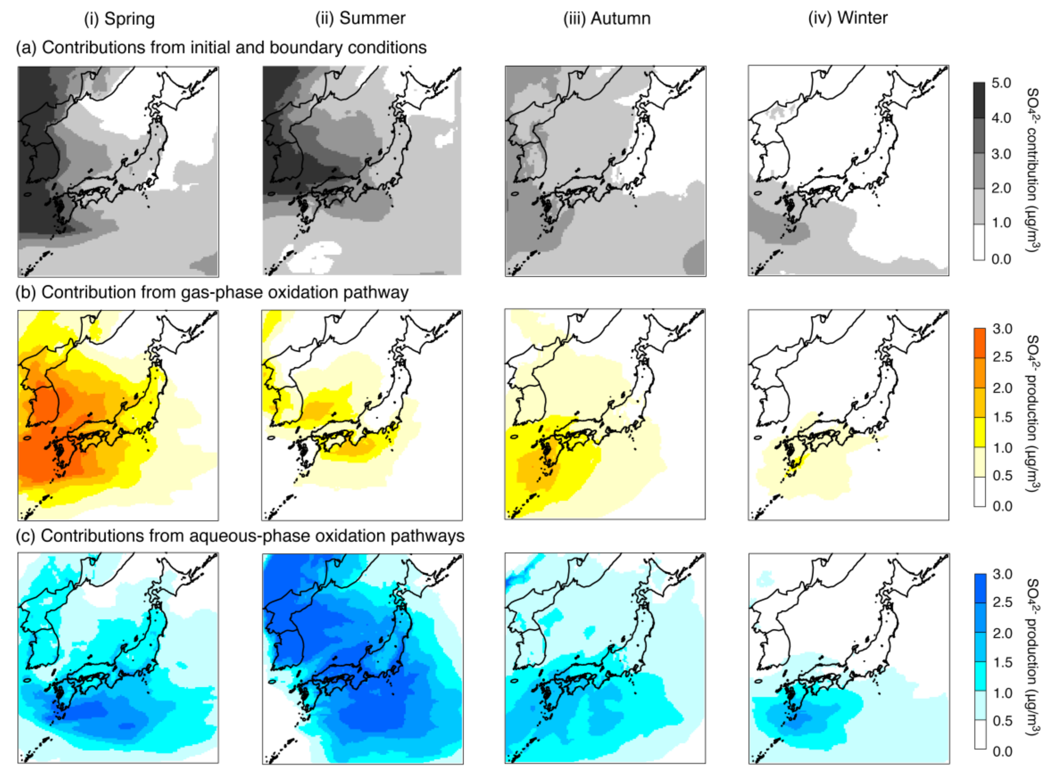
To investigate the modeled SO42− behavior further, the contributions of the initial and boundary conditions and production via the gas and aqueous phases were estimated based on STM. The seasonal averaged spatial distributions are shown in Figure 4, and the domain-averaged concentrations and contributions are summarized in Table 2. Throughout the year, there were intrusions from a higher contribution from the western boundary. This contribution was higher than 5.0 μg/m3 in spring and summer in Western Japan (Figure 4a). For the domain average, the absolute values of the contributions of the initial and boundary conditions changed according to the season, but the relative contributions were almost 50% (Table 2). The spatial distributions of SO42− production from gas- and aqueous-phase oxidation mostly coincided over Japan. Production via gas-phase oxidation was more important during spring, and production via aqueous-phase oxidation was more important during summer. For the domain-averaged contribution, the gas-phase oxidation pathway made the lowest contribution in summer of below 10% and the highest in spring of above 25% (Table 2). In coastal areas, although contributions from emissions mainly attributed to ships were found, their impact on the domain-averaged value was limited and lower than 0.1 μg/m3 (1.1–3.3%). In winter, gas-phase production was smaller because of the low OH concentration, and aqueous-phase production was more important for producing SO42− [34]. Over the domain, the contributions from the gas-phase and aqueous-phase oxidation pathways were 19.3% and 28.7% during winter, respectively.
Five aqueous-phase oxidation pathways can be tracked in STM. Production by H2O2, O3, and O2 with Fe- and Mn-catalyzed oxidation is displayed in Figure 5 as a fraction of the total aqueous-phase production shown in Figure 4c. Production by MHP and PAA was minor (not shown). The H2O2 aqueous-phase oxidation pathway was identified as the main pathway as it is the most effective oxidant [25,35,36]. Over Japan, oxidation by H2O2 accounted for more than 90% in most areas and oxidation by O3 accounted for less than 30% of the aqueous-phase oxidation. Production via the Fe- and Mn-catalyzed O2 oxidation pathway during spring, summer, and autumn was negligible, whereas during winter, it accounted for about 30–40% of production over the Asian continent. This was caused by the assignment of coarse-mode Fe and Mn from anthropogenic coarse-mode aerosol. However, the concentration over this area was lower than 2.0 μg/m3 (Figure 2iv). Over Japan, although Fe and Mn were simulated, they were substantially underestimated, and this led to the lower production by Fe- and Mn-catalyzed oxidation by O2. Based on these CMAQ-STM results, the refinement of aqueous-phase Fe- and Mn-catalyzed oxidation by O2 is presented in the next section.
4.2. Sensitivity Simulation of the Fe and Mn Treatment
In this section, three sensitivity simulations are presented. A brief summary of the simulations is shown in Table 3.
4.2.1. Adjustment of Fe and Mn Concentrations
The base-case simulation in CMAQ version 5.0.2 based on the J-STREAM emission framework showed that the model underestimated Fe and Mn concentrations substantially throughout the seasons. A sensitivity analysis where the Fe and Mn concentrations were adjusted to the observed concentrations was conducted. As a simplified approach, the moderate correlation between the model and observations allowed the factors to adjust between the mean of the model and the mean of observation during each season to be used to adjust the model results. These factors were 7.55, 7.35, 6.17, and 6.28 for Fe, and 21.10, 23.33, 20.34, and 20.18 for Mn during spring, summer, autumn, and winter, respectively. As Fe and Mn are primary pollutants, the factor in each season was applied to increase the emission intensity. Hereafter, we call this sensitivity simulation of the adjustment of the Fe and Mn concentrations sensitivity simulation A.
Changes in SO42− concentration and SO42− production from aqueous-phase oxidation are shown in Figure 6 as the relative change from the base-case simulation. These results indicated that the effective increase in SO42− production from aqueous-phase oxidation, and the consequent increase in SO42− concentration only occurred during winter. The increase in SO42− production from aqueous-phase oxidation of over 5% when compared with the base-case simulation was found over the Kansai and Kanto regions, and resulted in a 1–2% increase in SO42− concentration. In other seasons, Fe- and Mn-catalyzed oxidation by O2 increased; however, this was offset by the decrease in oxidation by O3. The decrease in aqueous-phase oxidation by O3 was related to the slight increase in the atmospheric concentration of O3. In addition, aqueous-phase oxidation by H2O2 was identified as the most important pathway. As a result, the differences were small and almost within ±1% when compared with the base-case simulation. The improvements in model performance during winter through the three sensitivity experiments are listed in Table 4. The increase in SO42− concentration over the whole of Japan was 0.7% (0.016 μg/m3). MFE did not improve, but MFB was improved slightly by 0.4%. The percentages within factors of 2 and 3 were increased by 0.7% and 0.2%, respectively, but there was no increase in the percentages within a factor of 5.
4.2.2. Increase in the Fe and Mn Solubilities
Sensitivity simulation A demonstrated that adjusting the Fe and Mn concentrations increased the SO42− concentration via aqueous-phase oxidation. The aqueous-phase Fe- and Mn-catalyzed O2 oxidation pathway in CMAQ makes various assumptions about the solubility and diurnal variation of Mn and Fe. The solubility and oxidation state of Fe are highly variable and depend on a number of factors including the origin of the aerosol and time of day. In the diurnal cycle, Fe mainly exists as Fe(II) during the day and Fe(III) at night [37,38]. Mn is typically more soluble than Fe and exists mainly as Mn(II) in cloud and fog droplets. In CMAQ version 5.0.2, the solubilities of Fe and Mn are kept constant at 10% and 50%, respectively; Fe(III) is assumed to be 10% of the dissolved Fe during the day and 90% at night; and all dissolved Mn is assumed to be Mn(II). These assumptions were based on the research for the global model in GEOS-Chem [11]. Considering these treatments for solubility and dissolution in CMAQ modeling, the observation results over Japan (Table 2) suggest that the assumption of the background concentrations of Fe(III) and Mn(II) in the previous CMAQ version were suitable night time values for the Fe- and Mn-catalyzed O2 oxidation pathway.
More soluble Fe was found in anthropogenic source regions when compared with those areas with high levels of natural dust emissions [37]. The current CMAQ model does not include the solubilities for anthropogenic and dust emission sources; hence, here we considered the solubilities separately. In our forthcoming study, we aim to include a windblown dust simulation in Asia. In addition, we used the maximum solubility for Fe and Mn based on the research on GEOS-Chem [11]. The sensitivity experiment with the GEOS-Chem model revealed that SO42− production was increased by the increase in solubility [11]. These revisions are listed in Table 5. Hereafter, we call this simulation sensitivity simulation B. As the increase in SO42− production was small except for in winter, sensitivity simulation B was undertaken during summer and winter.
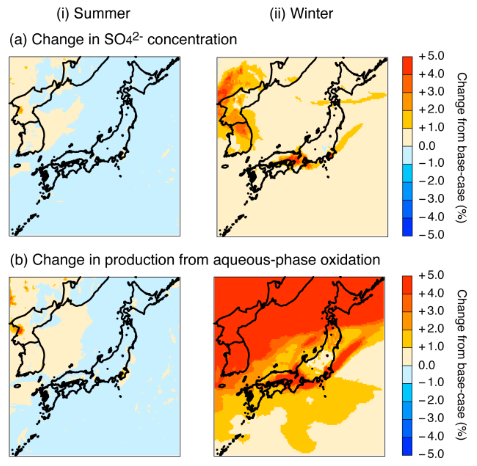
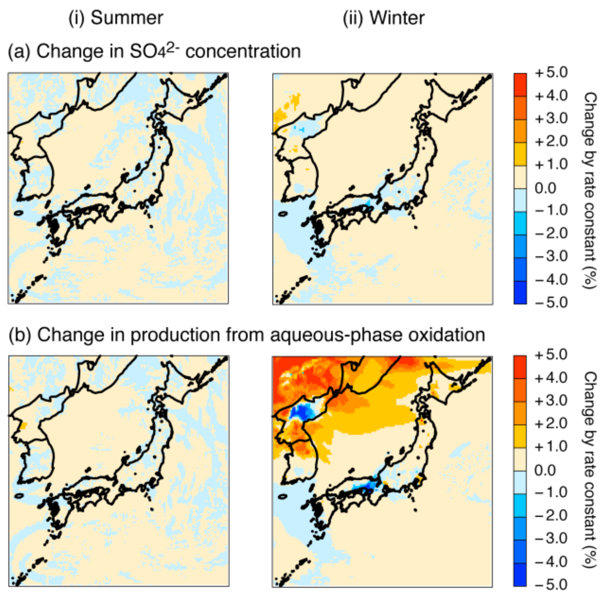
Changes in SO42− concentration and SO42− production resulting from the aqueous-phase oxidation contribution in sensitivity simulation B are shown in Figure 7 as relative changes from the base-case simulation. The increase in SO42− concentration was also almost within ±1% during summer, whereas it was over 5% over the Asian continent (including Northeast China and the north of the Republic of Korea) and Kansai and Kanto regions in Japan. The increase in aqueous-phase oxidation was larger than 5% over most of domain 2. This caused an increase of +2.4% (0.058 μg/m3) in SO42− concentration over the whole of domain 2 (Table 4). MFB and MFE were improved by 1.5% and 0.6%, respectively, and the percentages within factors of 2, 3, and 5 were also increased by 0.9%, 0.5%, and 0.4%, respectively. This result showed that the solubility in the aqueous-phase reactions is an important factor for refining the modeled aqueous-phase oxidation in winter.
4.2.3. Revision of the Fe and Mn Rate Constant
The sensitivity simulations with the adjusted Fe and Mn concentrations and solubilities demonstrated the importance of these treatments in increasing the SO42− concentration during winter. The rate constant expression of the aqueous-phase Fe- and Mn-catalyzed O2 oxidation pathway used by CMAQ version 5.0.2 or later is
where k1 = 750 M−1 s−1, k2 = 2600 M−1 s−1, and k3 = 1.0 × 10¹⁰ M−2 s−1. The sulfate inhibition effect is also modeled by
which is derived from the ionic strength dependence [10]. This formula suggests that the synergistic existence of Fe and Mn contributes significantly to this oxidation production. In another study, this synergistic effect is expressed by considering the pH dependency
where k3′ = 2.51 × 10¹³ M−1 s−1 and k3′′ = 3.72 × 10⁷ M−1 s−1 [39]. Equations (4) and (3) are used for the oxidation pathway in CAMx [40]. In sensitivity simulation C, Equation (2) is replaced with Equation (4) in CMAQ to model the synergistic existence of Fe and Mn.
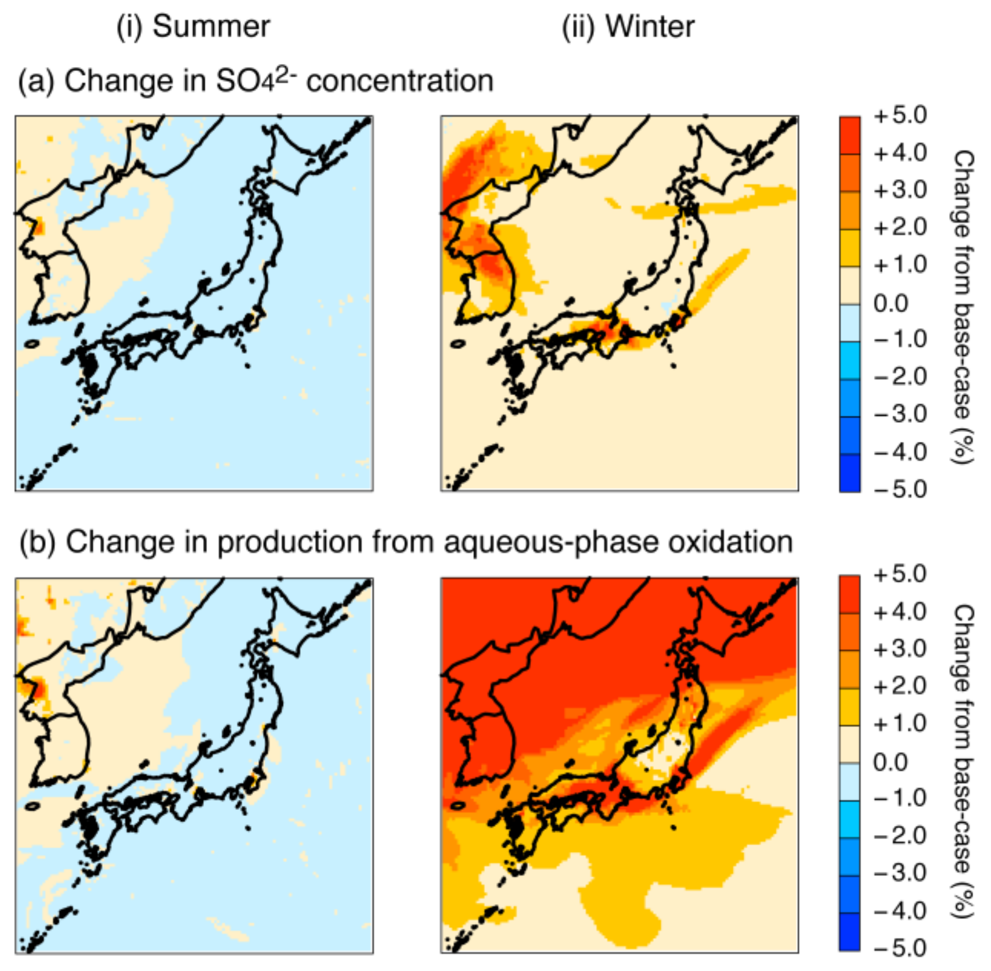
Changes in SO42− concentration and production from aqueous-phase oxidation in sensitivity simulation C are shown in Figure 8 as relative changes from the base-case simulation. The averaged spatial distribution results were similar to those of sensitivity simulation B (Figure 7). Comparing the results with the observations showed further improvements (Table 4). The averaged concentration was increased by 3.5% (0.084 μg/m3) when compared with the base-case simulation. MFB and MFE were improved by 3.6% and 2.6%, respectively. The percentages within factors of 2, 3, and 5 were also increased by 3.2%, 2.3%, and 1.7%, respectively.
The differences caused by the rate constant revision and determined by comparing sensitivity simulations B and C were analyzed further (Figure 9). The effect of the rate constant on SO42− concentration was small and almost within ±1% on average. For SO42− aqueous-phase production, the differences were complicated; positive signs (i.e., including pH dependency increased production) were found over most of the Asian continent, and negative signs (i.e., including pH dependency decreased production) were found over parts of Northern Korea and Japan such as the Kansai region. Further refinement of the modeled pH is required as pH is affected by trace elements, but the evaluation of these elements is limited as we have highlighted in this study of Fe and Mn. The recent framework for the aqueous-phase solver in CMAQ also offers valuable insights, especially for the short-term (e.g., hourly) model performance [41].
5. Conclusions
The Japanese model inter-comparison study, J-STREAM, found that although SO42− is generally well captured by models, it is underestimated during winter. In the present study, we presented a way to improve the modeled SO42− concentration marginally during winter in Japan. Although CMAQ can treat one gas-phase and five aqueous-phase reactions for SO42− production, the Fe- and Mn-catalyzed oxidation by O2 cannot always be adequately represented. This is because the current emission inventories lack information about trace elements. The base-case simulation based on the latest emissions from Japan showed that Fe and Mn levels were substantially underestimated throughout the year. Therefore, three sensitivity simulations incorporating STM were performed: (A) adjusting the modeled Fe and Mn concentrations to observed concentrations; (B) increasing the solubility of Fe and Mn, in addition to A; and (C) revising the rate constant to include the pH dependency, in addition to A and B. Sensitivity simulation A revealed that adjusting the Fe and Mn concentrations increased SO42− aqueous-phase production, and consequently SO42− concentration, only during winter. Sensitivity simulation B demonstrated that increasing Fe and Mn solubilities led to a further increase in SO42− concentration in winter. Increases in SO42− aqueous-phase production larger than 5% were found over most of the model domain around Japan. As a result, the effect of increasing the concentrations and solubilities of Fe and Mn was an increase in SO42− concentration larger than 2.4% (0.058 μg/m3) over the whole of Japan when compared with the base-case simulation. Sensitivity simulation C improved the model performance further with an increase in SO42− concentration of 3.5% (0.084 μg/m3) when compared with the base-case simulation. Comparing the results of revising the rate constant revealed that pH dependency caused complex changes in the production of SO42− via aqueous-phase oxidation. Through these sensitivity simulations, we partly improved the underestimation of modeled SO42− during winter on average. This approach increased SO42− concentration further, especially for stagnation conditions in winter as trace elements accumulate under these weather conditions. However, the model still underestimated SO42− concentrations. Although we did not include the mineral dust simulation, Fe and Mn from natural dust could contribute to increasing the SO42− production via aqueous-phase oxidation, as shown in this study, in addition to heterogeneous chemistry [42,43,44]. Recent studies have focused on the importance of heterogeneous chemistry [45,46], NO2 chemistry [42,47], and reactive nitrogen chemistry [48] for the production of SO42− in winter haze episodes in China. It is necessary to incorporate these findings to improve the model performance during winter. Although the emission inventory must be refined, the uncertainty of SO2 emissions may be small based on the current understanding of the Asian emission inventory [49]. Instead, we can improve our overall knowledge of the oxidation capacity in the atmosphere via the refinement of other species, especially of volatile organic compounds. The first-phase model inter-comparison used common input datasets for meteorology. To explore the meteorological impacts such as the vertical distribution is one of the targets of the second-phase. Furthermore, comprehensive analysis including deposition processes is essential for evaluating the budget of sulfur compounds (i.e., SO2 and SO42−). We intend to tackle these topics in future work.
Our study also indicated the importance of including trace elements in the emission inventory. In most global or Asian inventories, only black and organic carbon are included as the speciation of aerosol components. For China, one of the largest emission sources in the world, many studies have only focused on one or several trace metals, particularly toxic heavy metals [50,51,52,53,54,55]. The development of trace elements in emission inventories and model evaluations is required. Our approach for Japan should be applied to China given that trans-boundary SO42− may have an impact over East Asia [26,27,28,29,30]. The refinement of the modeled aqueous-phase Fe- and Mn-catalyzed oxidation by O2 over China may further improve the model performance during winter over both China and downwind regions. Finally, a recent study quantified the role of iron oxide (FeOx) as a contributor to atmospheric heating [56]. Understanding trace elements such as Fe, and ongoing simulations are essential areas of research in air quality and regional climate change.
Acknowledgments
This research was supported by the Environment Research and Technology Development Fund (5-1601) of the Environmental Restoration and Conservation Agency. The authors appreciate the helpful comments on the coarse-mode speciation of Fe and Mn in CMAQ from Golam Sarwar, Sergey Napelenok, and Kathleen Fahey at the US Environmental Protection Agency.
Author Contributions
Syuichi Itahashi developed the sub-model for the aqueous-phase reaction and wrote this paper; Kazuyo Yamaji was the sub-leader of the model inter-comparison, and prepared the meteorological inputs and initial and boundary conditions; Hiroshi Hayami was the sub-leader of the inorganic aerosol measurements and contributed to the sub-model development; Satoru Chatani was the leader of the J-STREAM project, and prepared the emission inputs and discussed the sub-model development.
Conflicts of Interest
The authors declare no conflict of interest.
References
- Chatani, S.; Yamaji, K.; Sakurai, T.; Itahashi, S.; Shimadera, H.; Kitayama, K.; Hayami, H. Overview of model inter-comparison in Japan’s study for reference air quality modeling (J-STREAM). Atmosphere 2018, 9, 19. [Google Scholar] [CrossRef]
- Yamaji, K.; Kobe University, Kobe, Hyogo Prefecture, Japan. Personal communication, 2018.
- Tesche, T.W.; Morris, R.; Tonnesen, G.; McNally, D.; Boylan, J.; Brewer, P. CMAQ/CAMx annual 2002 performance evaluation over the eastern US. Atmos. Environ. 2006, 40, 4906–4919. [Google Scholar] [CrossRef]
- Zhang, Y.; Olsen, K.M.; Wang, K. Fine-scale modeling of agricultural air quality over the Southeastern United States using two air quality models. Part I. Application and Evaluation. Aerosol Air Qual. Res. 2013, 13, 1231–1252. [Google Scholar] [CrossRef]
- CMAQ v5.0 Sulfur Chemistry. Available online: https://www.airqualitymodeling.org/index.php/CMAQv5.0_Sulfur_Chemistry (accessed on 20 January 2018).
- Sander, S.P. Chemical Kinetics and Photochemical Data for Use in Atmospheric Studies Evaluation Number 15; JPL Publication: Pasadena, CA, USA, 2006. [Google Scholar]
- Whitten, G.Z.; Heo, G.; Kimura, Y.; McDonald-Buller, E.; Allen, D.T.; Carter, W.P.L.; Yarwood, G. A new condensed toluene mechanism for carbon bond CB05-TU. Atmos. Environ. 2010, 44, 5346–5355. [Google Scholar] [CrossRef]
- Carter, W.P.L. Development of the SAPRC-07 chemical mechanism. Atmos. Environ. 2010, 44, 5324–5335. [Google Scholar] [CrossRef]
- Jacobson, M. Development and application of a new air pollution modeling system-II. Aerosol module structure and design. Atmos. Environ. 1997, 31, 131–144. [Google Scholar] [CrossRef]
- Martin, R.L.; Good, T.W. Catalyzed oxidation of sulfur dioxide in solution: The iron-manganese synergism. Atmos. Environ. 1991, 25, 2395–2399. [Google Scholar] [CrossRef]
- Alexander, B.; Park, R.J.; Jacob, D.J.; Gong, S. Transition metal-catalyzed oxidation of atmospheric sulfur: Global implications for the sulfur budget. J. Geophys. Res. 2009, 114. [Google Scholar] [CrossRef]
- Fountoukis, C.; Nenes, A. ISORROPIA II: A computationally efficient thermodynamic equilibrium model for K+-Ca2+-Mg2+-NH4+-Na+-SO42−-NO3--Cl−-H2O aerosols. Atmos. Chem. Phys. 2007, 7, 4639–4659. [Google Scholar] [CrossRef]
- Reff, A.H.; Bhave, P.; Simon, H.; Pace, T.; Pouliot, G.; Mobley, D.; Houyoux, M. Emissions inventory of PM2.5 trace elements across the United States. Environ. Sci. Technol. 2009, 43, 5790–5796. [Google Scholar] [CrossRef]
- Appel, K.W.; Pouliot, G.A.; Simon, H.; Sarwar, G.; Pye, H.O.T.; Napelenok, S.L.; Akhtar, F.; Roselle, S.J. Evaluation of dust and trace metal estimates from the Community Multiscale Air Quality (CMAQ) model version 5.0. Geosci. Model Dev. 2013, 6, 883–899. [Google Scholar] [CrossRef]
- Simon, H.; Beck, L.; Bhave, P.V.; Divita, F.; Hsu, Y.; Luecken, D.; Mobley, J.D.; Pouliot, G.A.; Reff, A.; Sarwar, G.; et al. The development and uses of EPA’s SPECIATE database. Atmos. Pollut. Res. 2010, 1, 196–206. [Google Scholar] [CrossRef]
- Upadhyay, N.; Clements, A.L.; Fraser, M.P.; Sundblom, M.; Solomon, P.; Herckes, P. Size-differentiated chemical composition of re-suspended soil dust from the desert southwest United States. Aerosol Air Qual. Res. 2015, 15, 387–398. [Google Scholar] [CrossRef]
- Crippa, M.; Janssens-Maenhout, G.M.; Dentener, F.; Guizzardi, D.; Sindelarova, K.; Muntean, M.; Van Dingenen, R.; Granier, C. Forty years of improvements in European air quality; regional policy-industry interactions with global impacts. Atmos. Chem. Phys. 2016, 16, 3825–3841. [Google Scholar] [CrossRef] [Green Version]
- Janssens-Maenhout, G.; Crippa, M.; Guizzardi, F.; Dentener, F.; Muntean, M.; Pouliot, G.; Keating, T.; Zhang, Q.; Kurokawa, J.; Wankmuller, R.; et al. HTAP_v2.2: A mosaic of regional and global emission grid maps for 2008 and 2010 to study hemispheric transport of air pollution. Atmos. Chem. Phys. 2015, 15, 11411–11432. [Google Scholar] [CrossRef] [Green Version]
- Kurokawa, J.; Ohara, T.; Morikawa, T.; Hanayama, S.; Janssens-Maenhout, G.; Fukui, T.; Kawashima, K.; Akimoto, H. Emissions of air pollutants and greenhouse gases over Asian regions during 2000–2008: Regional Emission inventory in ASia (REAS) version 2. Atmos. Chem. Phys. 2013, 13, 11019–11058. [Google Scholar] [CrossRef]
- Chatani, S.; Morikawa, T.; Nakatsuka, S.; Matsunaga, S.; Minoura, H. Development of a framework for a high-resolution, three-dimensional regional air quality simulation and its application to predicting future air quality over Japan. Atmos. Environ. 2011, 45, 1383–1393. [Google Scholar] [CrossRef]
- Chatani, S.; Morino, Y.; Shimadera, H.; Hayami, H.; Mori, Y.; Sasaki, K.; Kajino, M.; Yokoi, T.; Morikawa, T.; Ohara, T. Multi-model analyses of dominant factors influencing elemental carbon in Tokyo metropolitan area of Japan. Aerosol Air Qual. Res. 2014, 14, 396–405. [Google Scholar] [CrossRef]
- Shimadera, H.; Hayami, H.; Chatani, S.; Morikawa, T.; Morino, Y.; Mori, Y.; Yamaji, K.; Nakatsuka, S.; Ohara, T. Urban air quality model inter-comparison study in Japan (UMICS) for improvement of PM2.5 simulation. Asian J. Atmos. Environ. 2017, in press. [Google Scholar]
- CMAQ v5.0.2 Sulfur Tracking. Available online: https://www.airqualitymodeling.org/index.php/ (accessed on 20 January 2018).
- Mathur, R.; Roselle, S.; Pouliot, G.; Sarwar, G. Diagnostic analysis of the three-dimensional sulfur distributions over the Eastern United States using the CMAQ model and measurements from the ICARTT field experiment. In Air pollution Modeling and Its Application XIX; NATO Science for Peace and Security Series; Springer: Dordrecht, The Netherlands, 2008; Volume 5, pp. 496–504. [Google Scholar] [CrossRef]
- Stein, A.F.; Saylor, R.D. Sensitivities of sulfate aerosol formation and oxidation pathways on the chemical mechanism employed in simulations. Atmos. Chem. Phys. 2012, 12, 8567–8574. [Google Scholar] [CrossRef]
- Itahashi, S.; Uno, I.; Yumimoto, K.; Irie, H.; Osada, K.; Ogata, K.; Fukushima, H.; Wang, Z.; Ohara, T. Interannual variation in the fine-mode MODIS aerosol optical depth and its relationship to the changes in sulfur dioxide emissions in China between 2000 and 2010. Atmos. Chem. Phys. 2012, 12, 2631–2640. [Google Scholar] [CrossRef] [Green Version]
- Itahashi, S.; Uno, I.; Kim, S.-T. Source contributions of sulfate aerosol over East Asia estimated by CMAQ-DDM. Environ. Sci. Technol. 2012, 46, 6733–6741. [Google Scholar] [CrossRef] [PubMed]
- Itahashi, S.; Hayami, H.; Yumimoto, K.; Uno, I. Chinese province-scale source apportionments for sulfate aerosol in 2005 evaluated by the tagged tracer method. Environ. Pollut. 2017, 220, 1366–1375. [Google Scholar] [CrossRef] [PubMed]
- Itahashi, S.; Hatakeyama, S.; Shimada, K.; Tatsuta, S.; Taniguchi, Y.; Chan, C.K.; Kim, Y.-P.; Lin, N.-H.; Takami, A. Model estimation of sulfate aerosol source collected at Cape Hedo during an intensive campaign in October–November, 2015. Aerosol Air Qual. Res. 2017, 17, 3079–3090. [Google Scholar] [CrossRef]
- Itahashi, S. Toward synchronous evaluation of source apportionments for atmospheric concentration and deposition of sulfate aerosol over East Asia. J. Geophys. Res. 2018, 123. [Google Scholar] [CrossRef]
- Boylan, J.W.; Russell, A.G. PM and light extinction model performance metrics, goals, and criteria for three-dimensional air quality models. Atmos. Environ. 2006, 40, 4946–4959. [Google Scholar] [CrossRef]
- Liu, C.L.; Zhang, B.; Shen, Z.B. Spatial and temporal variability of trace metals in aerosol from the desert region of China ant the Yellow Sea. J. Geophys. Res. 2002, 107. [Google Scholar] [CrossRef]
- Hao, Y.; Guo, Z.; Yang, Z.; Fang, M.; Feng, J. Seasonal variations and sources of various elements in the atmospheric aerosols in Qingdao, China. Atmos. Res. 2007, 85, 27–37. [Google Scholar] [CrossRef]
- Itahashi, S.; Uno, I.; Osada, K.; Kamiguchi, Y.; Yamamoto, S.; Tamura, K.; Wang, Z.; Kurosaki, Y.; Kanaya, Y. Nitrate transboundary heavy pollution over East Asia in winter. Atmos. Chem. Phys. 2017, 17, 3823–3843. [Google Scholar] [CrossRef]
- Seinfeld, J.H.; Pandis, S.N. Atmospheric Chemistry and Physics—From Air Pollution to Climate Change, 2nd ed.; John Wiley & Sons: New York, NY, USA, 2006. [Google Scholar]
- Walcek, C.J.; Taylor, G.R. A theoretical method for computing vertical distributions of acidity and sulfate production within cumulus clouds. J. Atmos. Sci. 1986, 43, 339–355. [Google Scholar] [CrossRef]
- Siefert, R.L.; Johansen, A.M.; Hoffman, M.R.; Pehkonen, S.O. Measurements of trace metal (Fe, Cu, Mn, Cr) oxidation states in fog and stratus clouds. J. Air Waste Manag. Assoc. 1998, 48, 128–143. [Google Scholar] [CrossRef] [PubMed]
- Desboeufs, K.V.; Sofikitis, A.; Losno, R.; Colin, J.L.; Ausset, P. Dissolution and solubility of trace metals from natural and anthropogenic aerosol particulate matter. Chemosphere 2005, 58, 195–203. [Google Scholar] [CrossRef] [PubMed]
- Ibusuki, T.; Takeuchi, K. Sulfur dioxide oxidation by oxygen catalyzed by mixtures of manganese(II) and iron(III) in aqueous solutions at environmental reaction conditions. Atmos. Environ. 1987, 21, 1555–1560. [Google Scholar] [CrossRef]
- CAMx Overview. Available online: http://www.camx.com/about/default.aspx (accessed on 30 January 2018).
- Fahey, K.M.; Carlton, A.G.; Pye, H.O.T.; Baek, J.; Hutzell, W.T.; Stainier, C.O.; Baker, K.R.; Appel, K.W.; Jaoui, M.; Offenberg, J.H. A framework for expanding aqueous chemistry in the Community Multiscale Air Quality (CMAQ) model version 5.1. Geosci. Model Dev. 2017, 10, 1587–1605. [Google Scholar] [CrossRef]
- He, H.; Wang, Y.; Ma, Q.; Ma, J.; Chu, B.; Ji, D.; Tang, G.; Liu, C.; Zhang, H.; Hao, J. Pathways of sulfate enhancement by natural and anthropogenic mineral aerosols in China. Sci. Rep. 2014, 4, 4172. [Google Scholar] [CrossRef] [PubMed]
- Wang, Z.; Itahashi, S.; Uno, I.; Pan, X.L.; Osada, K.; Yamamoto, S.; Nishizawa, T.; Tamura, K.; Wang, Z. Modeling the long-range transport of particulate matters for January in East Asia using NAQPMS and CMAQ. Aerosol Air Qual. Res. 2017, 17, 3065–3078. [Google Scholar] [CrossRef]
- Fu, X.; Wang, S.; Chang, X.; Cai, S.; Xing, J.; Hao, J. Modeling analysis of secondary inorganic aerosols over China: Pollution characteristics, and meteorological and dust impacts. Sci. Rep. 2016, 6, 35992. [Google Scholar] [CrossRef] [PubMed]
- Zheng, B.; Zhang, Q.; Zhang, Y.; He, K.B.; Wang, K.; Zheng, G.J.; Duan, F.K.; Ma, Y.L.; Kimoto, T. Heterogeneous chemistry: A mechanism missing in current models to explain secondary inorganic aerosol formation during January 2013 haze episode in North China. Atmos. Chem. Phys. 2015, 15, 2031–2049. [Google Scholar] [CrossRef]
- Li, G.; Bei, N.; Cao, J.; Huang, R.; Wu, J.; Feng, T.; Wang, Y.; Liu, S.; Zhang, Q.; Tie, X.; et al. A possible pathway for rapid growth of sulfate during haze days in China. Atmos. Chem. Phys. 2017, 17, 3301–3316. [Google Scholar] [CrossRef]
- Wang, G.; Zhang, R.; Gomez, M.E.; Yang, L.; Levy Zamora, M.; Hu, M.; Lin, Y.; Peng, J.; Guo, S.; Meng, J.; et al. Persistent sulfate formation from London Fog to Chinese haze. Proc. Natl. Acad. Sci. USA 2016, 113, 13630–13635. [Google Scholar] [CrossRef] [PubMed]
- Cheng, Y.; Zheng, G.; Wei, C.; Mu, Q.; Zheng, B.; Wang, Z.; Gao, M.; Zhang, Q.; He, K.; Carmichael, G.; et al. Reactive nitrogen chemistry in aerosol water as a source of sulfate during haze events in China. Sci. Adv. 2016, 2, e1601530. [Google Scholar] [CrossRef] [PubMed]
- Meng, L.; Kilmont, Z.; Zhang, Q.; Martin, R.V.; Zheng, B.; Heyes, C.; Cofala, J.; Zhang, Y.; He, K. Comparison and evaluation of anthropogenic emissions of SO2 and NOx over China. Atmos. Chem. Phys. 2018, 18, 3433–3456. [Google Scholar]
- Lei, Y.; Zhang, Q.; He, K.B.; Streets, D.G. Primary anthropogenic aerosol emission trends for China, 1990–2005. Atmos. Chem. Phys. 2011, 11, 931–954. [Google Scholar] [CrossRef] [Green Version]
- Tian, H.; Zhao, D.; Cheng, K.; Lu, L.; He, M.; Hao, J. Anthropogenic atmospheric emissions of antimony and its spatial distribution characteristics in China. Environ. Sci. Technol. 2012, 46, 3973–3980. [Google Scholar] [CrossRef] [PubMed]
- Shao, X.; Cheng, H.; Li, Q.; Lin, C. Anthropogenic atmospheric emissions of cadmium in China. Atmos. Environ. 2013, 79, 155–160. [Google Scholar] [CrossRef]
- Cheng, H.; Zhou, T.; Li, Q.; Lu, L.; Lin, C. Anthropogenic Chromium Emissions in China from 1990 to 2009. PLoS ONE 2014, 9, e87753. [Google Scholar] [CrossRef] [PubMed]
- Cheng, K.; Wang, Y.; Tian, H.; Gao, X.; Zhang, Y.; Wu, X.; Zhu, C.; Gao, J. Atmospheric Emission Characteristics and Control Policies of Five Precedent-Controlled Toxic Heavy Metals from Anthropogenic Sources in China. Environ. Sci. Technol. 2015, 49, 1206–1214. [Google Scholar] [CrossRef] [PubMed]
- Tian, H.Z.; Zhu, C.Y.; Gao, J.J.; Cheng, K.; Hao, J.M.; Wang, K.; Hua, S.B.; Wang, Y.; Zhou, J.R. Quantitative assessment of atmospheric emissions of toxic heavy metals from anthropogenic sources in China: Historical trend, spatial distribution, uncertainties, and control policies. Atmos. Chem. Phys. 2015, 15, 10127–10147. [Google Scholar] [CrossRef]
- Moteki, N.; Adachi, K.; Ohata, S.; Yoshida, A.; Harigaya, T.; Koike, M.; Kondo, Y. Anthropogenic iron oxide aerosols enhance atmospheric heating. Nat. Commun. 2017, 8, 15329. [Google Scholar] [CrossRef] [PubMed]
Figure 1.
Mapping of the lowermost-layer emissions of (a) SO2, (b) Fe, and (c) Mn. Rectangles indicate the Kansai region (left) and Kanto region (right).
Figure 1.
Mapping of the lowermost-layer emissions of (a) SO2, (b) Fe, and (c) Mn. Rectangles indicate the Kansai region (left) and Kanto region (right).
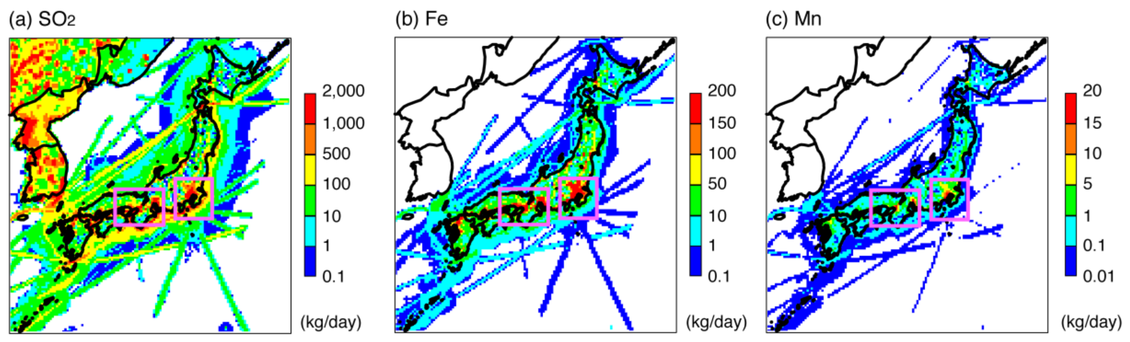
Figure 2.
Spatial distribution of SO42− concentration from (a) observations and (b) the model averaged over (i) spring, (ii) summer, (iii) autumn, and (iv) winter. Model results are from the base-case simulation.
Figure 2.
Spatial distribution of SO42− concentration from (a) observations and (b) the model averaged over (i) spring, (ii) summer, (iii) autumn, and (iv) winter. Model results are from the base-case simulation.
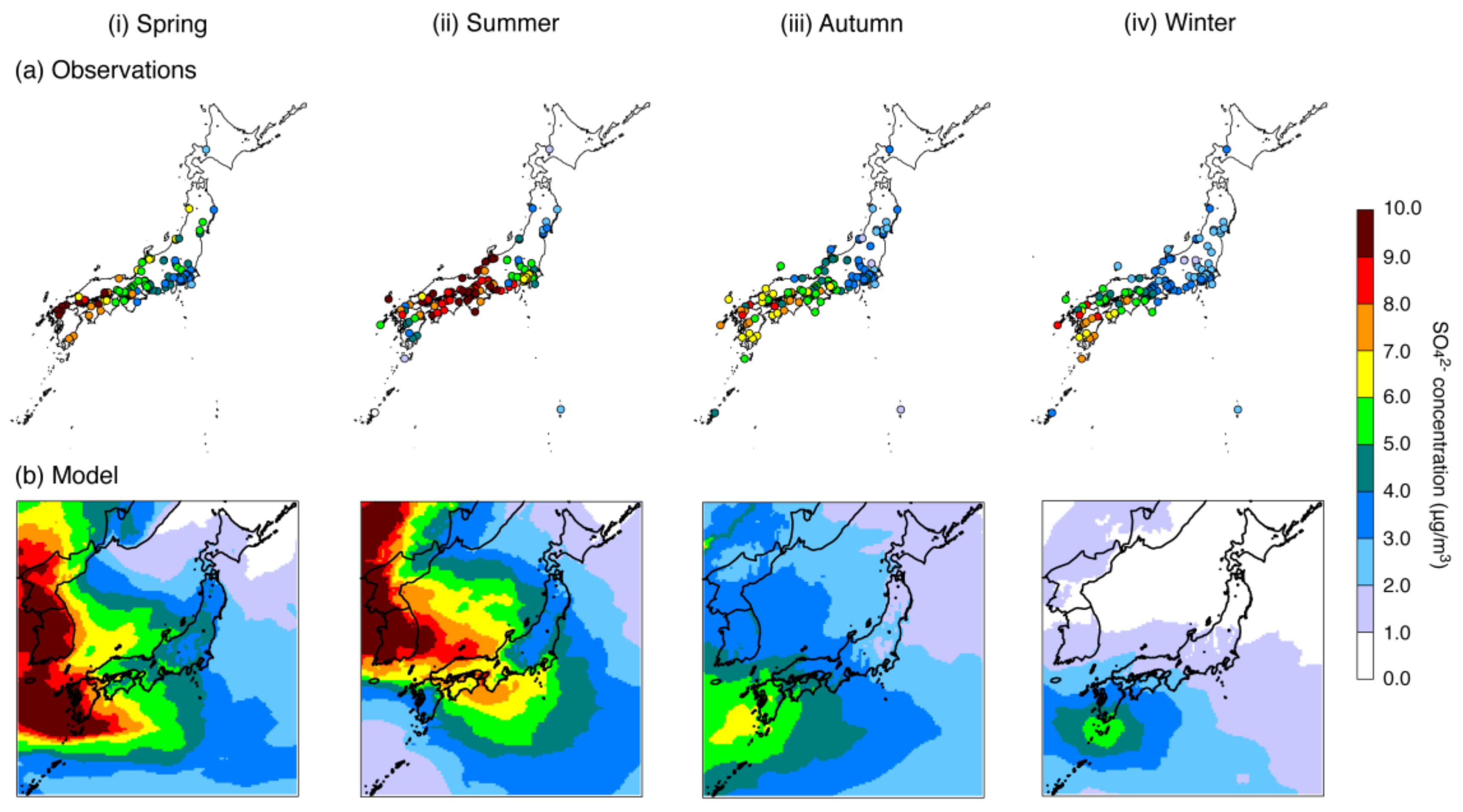
Figure 3.
Scatter-plot between observations and the model for daily (a) SO42−, (b) Fe, and (c) Mn concentrations during (i) spring, (ii) summer, (iii) autumn, and (iv) winter. Model results are from the base-case simulation. Note that (b,c) are illustrated with different scales of observations and model. Reference lines of 1:1, 1:2, 1:3, and 1:5 are inserted.
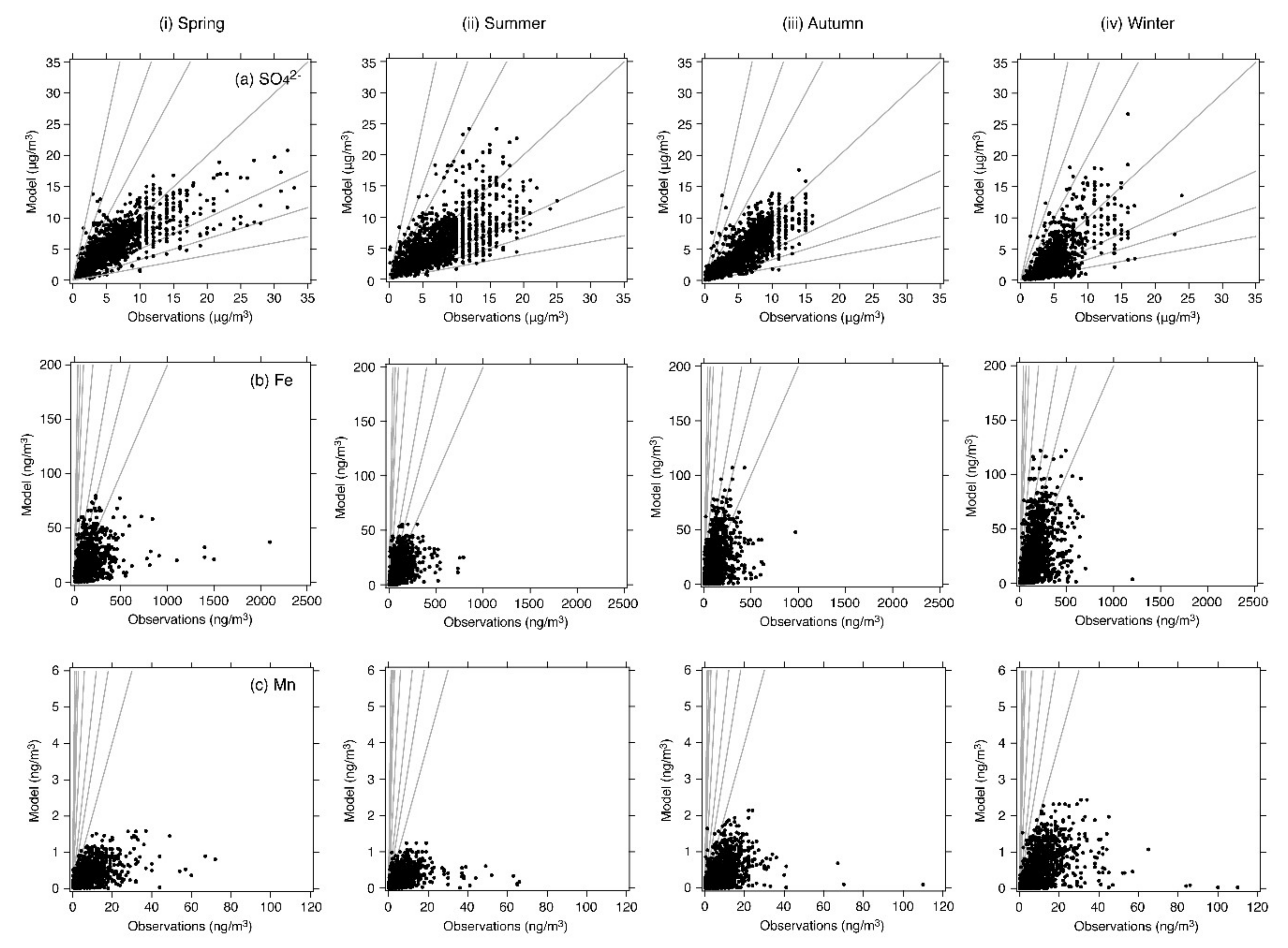
Figure 4.
Spatial distributions of (a) contributions from initial and boundary conditions, (b) contribution from the gas-phase oxidation pathway, and (c) contributions from the aqueous-phase oxidation pathways averaged over (i) spring, (ii) summer, (iii) autumn, and (iv) winter. Model results are from the base-case simulation with STM.

Figure 5.
Spatial distribution of production from aqueous-phase oxidation by (a) H2O2, (b) O3, and (c) O2 catalyzed by Fe and Mn averaged over (i) spring, (ii) summer, (iii) autumn, and (iv) winter. Model results are from the base-case simulation with STM.
Figure 5.
Spatial distribution of production from aqueous-phase oxidation by (a) H2O2, (b) O3, and (c) O2 catalyzed by Fe and Mn averaged over (i) spring, (ii) summer, (iii) autumn, and (iv) winter. Model results are from the base-case simulation with STM.
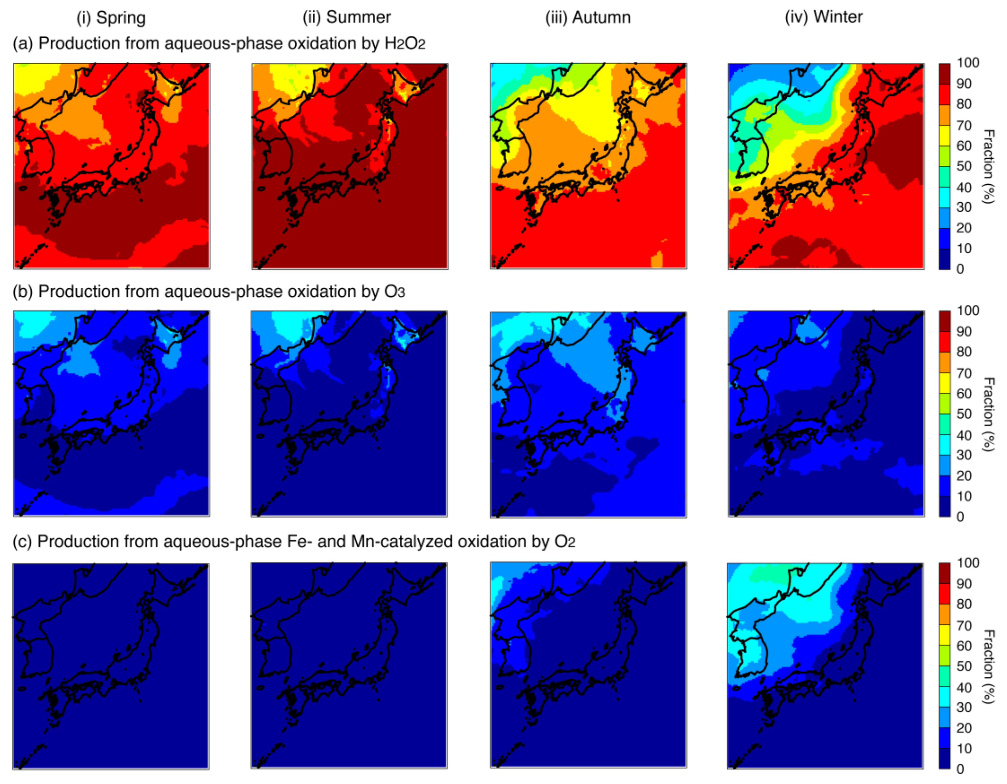
Figure 6.
Changes in (a) SO42− concentration and (b) production from aqueous-phase oxidation averaged over (i) spring, (ii) summer, (iii) autumn, and (iv) winter. Model results from sensitivity simulation A are compared with the base-case simulation.
Figure 6.
Changes in (a) SO42− concentration and (b) production from aqueous-phase oxidation averaged over (i) spring, (ii) summer, (iii) autumn, and (iv) winter. Model results from sensitivity simulation A are compared with the base-case simulation.
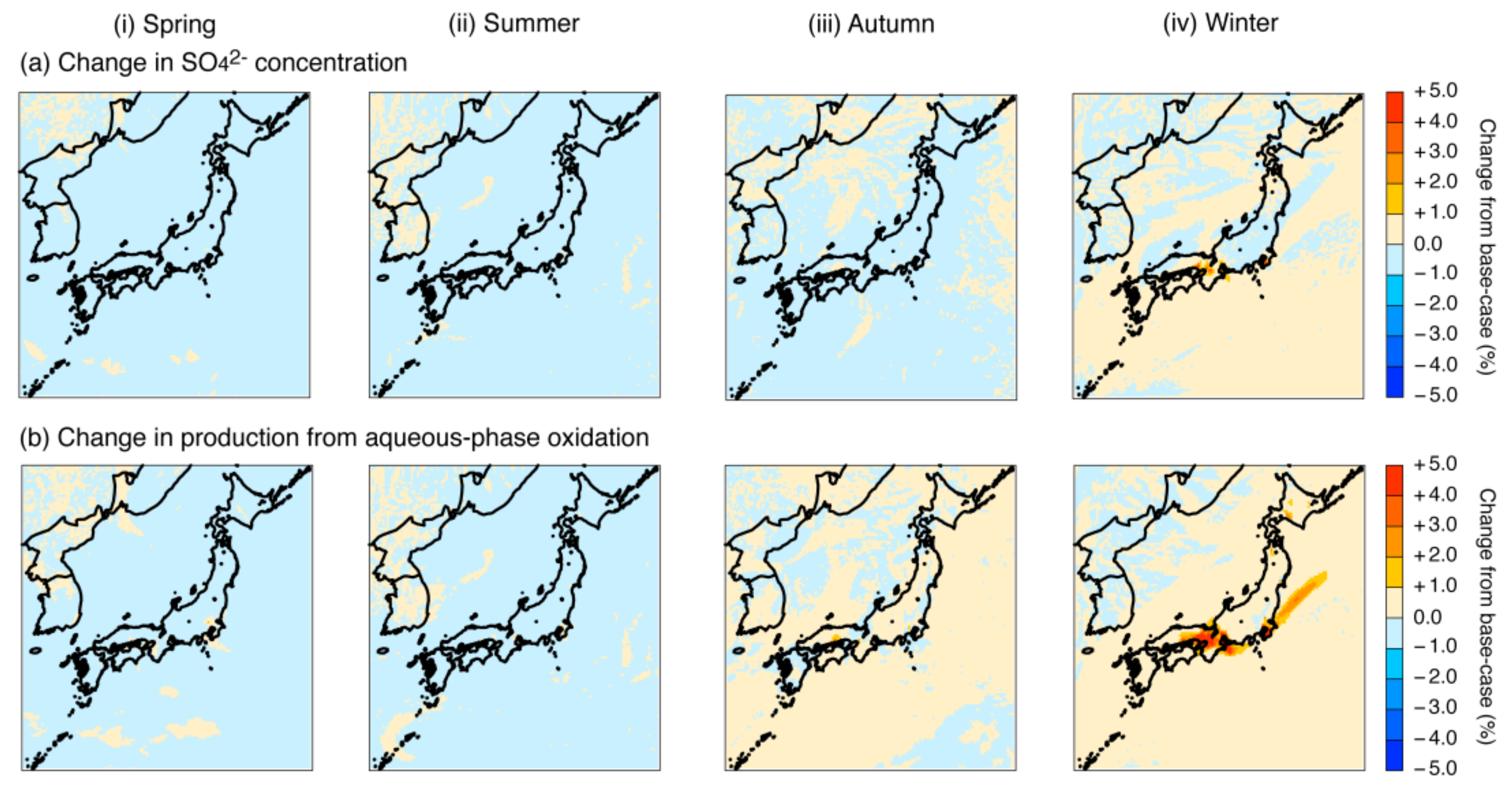
Figure 7.
Changes in (a) SO42− concentration and (b) production from aqueous-phase oxidation averaged over (i) summer and (ii) winter. Model results from sensitivity simulation B are compared with the base-case simulation.
Figure 7.
Changes in (a) SO42− concentration and (b) production from aqueous-phase oxidation averaged over (i) summer and (ii) winter. Model results from sensitivity simulation B are compared with the base-case simulation.

Figure 8.
Changes in (a) SO42− concentration and (b) production from aqueous-phase oxidation averaged over (i) summer and (ii) winter. Model results from sensitivity simulation C are compared with the base-case simulation.
Figure 8.
Changes in (a) SO42− concentration and (b) production from aqueous-phase oxidation averaged over (i) summer and (ii) winter. Model results from sensitivity simulation C are compared with the base-case simulation.

Figure 9.
Changes in (a) SO42− concentration and (b) production from aqueous-phase oxidation averaged over (i) summer and (ii) winter. Model results from sensitivity simulation C are compared with sensitivity simulation B; therefore, the differences caused by the rate constant are shown.
Figure 9.
Changes in (a) SO42− concentration and (b) production from aqueous-phase oxidation averaged over (i) summer and (ii) winter. Model results from sensitivity simulation C are compared with sensitivity simulation B; therefore, the differences caused by the rate constant are shown.


Table 1.
Statistical analysis of the model performance for SO42−, Fe, and Mn.
| Spring | Summer | Autumn | Winter | ||
|---|---|---|---|---|---|
| SO42− | N | 1583 | 1824 | 1910 | 1923 |
| Mean (observations) (μg/m3) | 5.78 | 7.18 | 4.89 | 4.00 | |
| Mean (model) (μg/m3) | 5.27 | 5.61 | 4.03 | 2.44 | |
| R | 0.78 (p < 0.001) | 0.69 (p < 0.001) | 0.84 (p < 0.001) | 0.73 (p < 0.001) | |
| MFB (%) | −4.9 | −22.3 | −19.0 | −72.2 | |
| MFE (%) | +33.0 | +40.2 | +39.7 | +79.3 | |
| % within a factor of 2 | 88.3 | 81.4 | 81.8 | 40.6 | |
| % within a factor of 3 | 96.8 | 95.4 | 93.6 | 63.1 | |
| % within a factor of 5 | 99.3 | 99.5 | 97.6 | 86.9 | |
| Fe | N | 1412 | 1669 | 1755 | 1763 |
| Mean (observation) (ng/m3) | 131.01 | 88.20 | 101.77 | 132.68 | |
| Mean (model) (ng/m3) | 17.35 | 12.00 | 16.48 | 21.14 | |
| R | 0.36 (p < 0.001) | 0.47 (p < 0.001) | 0.45 (p < 0.001) | 0.49 (p < 0.001) | |
| MFB (%) | –142.3 | –145.1 | –137.4 | –143.0 | |
| MFE (%) | +142.8 | +145.9 | +139.8 | +143.8 | |
| % within a factor of 2 | 5.5 | 4.4 | 8.4 | 6.3 | |
| % within a factor of 3 | 13.2 | 11.9 | 17.8 | 15.1 | |
| % within a factor of 5 | 33.4 | 30.3 | 37.1 | 33.6 | |
| Mn | N | 1324 | 1574 | 1657 | 1643 |
| Mean (observation) (ng/m3) | 7.76 | 5.93 | 7.23 | 8.88 | |
| Mean (model) (ng/m3) | 0.37 | 0.25 | 0.36 | 0.44 | |
| R | 0.48 (p < 0.001) | 0.37 (p < 0.001) | 0.42 (p < 0.001) | 0.45 (p < 0.001) | |
| MFB (%) | −174.0 | −178.1 | −175.6 | −178.0 | |
| MFE (%) | +174.2 | +178.2 | +175.9 | +178.1 | |
| % within a factor of 2 | 1.1 | 0.8 | 1.0 | 0.6 | |
| % within a factor of 3 | 2.4 | 1.4 | 2.4 | 1.3 | |
| % within a factor of 5 | 6.0 | 2.9 | 5.6 | 3.5 |
Table 2.
Domain-averaged concentration of SO42 and each contribution estimated by STM.
| Spring | Summer | Autumn | Winter | ||
|---|---|---|---|---|---|
| Concentration (μg/m3) | 4.39 | 4.59 | 3.10 | 1.62 | |
| Contribution (μg/m3) | Initial and boundary conditions | 2.17 (49.3%) 1 | 2.36 (51.4%) 1 | 1.52 (49.2%) 1 | 0.79 (48.7%) 1 |
| Gas-phase oxidation pathway | 1.12 (25.4%) 1 | 0.45 (9.8%) 1 | 0.61 (19.7%) 1 | 0.31 (19.3%) 1 | |
| Aqueous-phase oxidation pathways | 1.03 (23.5%) 1 | 1.73 (37.7%) 1 | 0.91 (29.5%) 1 | 0.46 (28.7%) 1 | |
| Emissions | 0.08 (1.8%) 1 | 0.05 (1.1%) 1 | 0.05 (1.6%) 1 | 0.05 (3.3%) 1 | |
1 Each relative contribution to the concentration is shown in brackets.
Table 3.
A brief summary of the three sensitivity simulations.
| Name | Description |
|---|---|
| Sensitivity simulation A | Fe and Mn concentrations are adjusted to observed concentrations |
| Sensitivity simulation B | Same as sensitivity simulation A, but the solubilities of Fe and Mn are increased (see Table 5) |
| Sensitivity simulation C | Same as sensitivity simulations B, but the rate constant expression of Fe- and Mn-catalyzed oxidation by O2 includes pH dependency |
Table 4.
Statistical analysis of model performance on SO42− during winter through three sensitivity experiments.
Table 4.
Statistical analysis of model performance on SO42− during winter through three sensitivity experiments.
| Sensitivity Simulation A | Sensitivity Simulation B | Sensitivity Simulation C | ||
|---|---|---|---|---|
| SO42− | Mean (model) (μg/m3) | 2.45 (+0.7%) 1 | 2.50 (+2.4%) 1 | 2.52 (+3.5%) 1 |
| R | 0.73 (p < 0.001) | 0.73 (p < 0.001) | 0.73 (p < 0.001) | |
| MFB (%) | –71.7 | –70.7 | –68.6 | |
| MFE (%) | +79.2 | +78.7 | +76.7 | |
| % within a factor of 2 | 41.3 | 41.5 | 43.8 | |
| % within a factor of 3 | 63.3 | 63.7 | 65.4 | |
| % within a factor of 5 | 86.9 | 87.3 | 88.6 |
1 The percentage changes from the base-case simulation are shown in brackets. Please refer to Table 1 for the base-case simulation.
Table 5.
Increase in the Fe and Mn solubilities in sensitivity simulation B.
| Base-Case | Sensitivity Simulation B | ||
|---|---|---|---|
| Fe | Solubility (anthropogenic) | 10% | 25% |
| Solubility (soil) | 10% | 1% | |
| Mn | Solubility | 50% | 100% |
© 2018 by the authors. Licensee MDPI, Basel, Switzerland. This article is an open access article distributed under the terms and conditions of the Creative Commons Attribution (CC BY) license (http://creativecommons.org/licenses/by/4.0/).
Share and Cite
MDPI and ACS Style
Itahashi, S.; Yamaji, K.; Chatani, S.; Hayami, H. Refinement of Modeled Aqueous-Phase Sulfate Production via the Fe- and Mn-Catalyzed Oxidation Pathway. Atmosphere 2018, 9, 132. https://doi.org/10.3390/atmos9040132
AMA Style
Itahashi S, Yamaji K, Chatani S, Hayami H. Refinement of Modeled Aqueous-Phase Sulfate Production via the Fe- and Mn-Catalyzed Oxidation Pathway. Atmosphere. 2018; 9(4):132. https://doi.org/10.3390/atmos9040132
Chicago/Turabian StyleItahashi, Syuichi, Kazuyo Yamaji, Satoru Chatani, and Hiroshi Hayami. 2018. "Refinement of Modeled Aqueous-Phase Sulfate Production via the Fe- and Mn-Catalyzed Oxidation Pathway" Atmosphere 9, no. 4: 132. https://doi.org/10.3390/atmos9040132
Note that from the first issue of 2016, this journal uses article numbers instead of page numbers. See further details here.