Seasonal Variability of Airborne Particulate Matter and Bacterial Concentrations in Colorado Homes
by

Nicholas Clements
1, 
Patricia Keady
1,
Joanne B. Emerson
2,
Noah Fierer
2,3 and
Shelly L. Miller
1,* 1
Department of Mechanical Engineering, College of Engineering and Applied Science, University of Colorado, Boulder, CO 80309, USA
2
Cooperative Institute for Research in Environmental Sciences, University of Colorado, Boulder, CO 80309, USA
3
Department of Ecology and Evolutionary Biology, University of Colorado, Boulder, CO 80309, USA
*
Author to whom correspondence should be addressed.
Atmosphere 2018, 9(4), 133; https://doi.org/10.3390/atmos9040133
Submission received: 5 February 2018
/
Revised: 25 March 2018
/
Accepted: 27 March 2018
/
Published: 2 April 2018
(This article belongs to the Special Issue Indoor Air Pollution)
Abstract
:Aerosol measurements were collected at fifteen homes over the course of one year in Colorado (USA) to understand the temporal variability of indoor air particulate matter and bacterial concentrations and their relationship with home characteristics, inhabitant activities, and outdoor air particulate matter (PM). Indoor and outdoor PM2.5 concentrations averaged (±st. dev.) 8.1 ± 8.1 μg/m3 and 6.8 ± 4.5 μg/m3, respectively. Indoor PM2.5 was statistically significantly higher during summer compared to spring and winter; outdoor PM2.5 was significantly higher for summer compared to spring and fall. The PM2.5 I/O ratio was 1.6 ± 2.4 averaged across all homes and seasons and was not statistically significantly different across the seasons. Average indoor PM10 was 15.4 ± 18.3 μg/m3 and was significantly higher during summer compared to all other seasons. Total suspended particulate bacterial biomass, as determined by qPCR, revealed very little seasonal differences across and within the homes. The qPCR I/O ratio was statistically different across seasons, with the highest I/O ratio in the spring and lowest in the summer. Using one-minute indoor PM10 data and activity logs, it was observed that elevated particulate concentrations commonly occurred when inhabitants were cooking and during periods with elevated outdoor concentrations.
1. Introduction
Air pollution impacts human health and quality of life [1]. The air quality in the indoor environment is especially important, as humans spend the majority of their time inside buildings. Indoor air quality (IAQ) is impacted by indoor emissions (cooking, cleaning, volatile organic compound (VOC) off-gassing), occupant activities, as well as infiltration of outdoor air pollution [2]. Ventilation conditions modulate indoor air pollutants by removing them through filtration and dilution but can also bring outdoor air pollutants into the built environment, especially when natural ventilation is used or mechanical ventilation filters are not adequate [3].
Residential IAQ is highly dependent on occupant activities, and activities such as cooking, home heating, cleaning, and opening windows or doors to increase natural ventilation modulate indoor pollutant concentrations. Cooking typically emits a large number of submicron particles, but emission characteristics such as particle size distribution and emitted organic species vary depending on appliance used, cooking oils used, and the type of food being prepared [4,5]. In many IAQ monitoring studies, the highest indoor aerosol concentrations occur during cooking or biomass burning events [6,7,8]. Vacuuming [9], dusting [10], and general occupant movement [11] can resuspend settled dust. Dust resuspension tends to emit more mass in the super-micron size range than the submicron range. Indoor particulate source apportionment studies indicate that road dust, soil dust, vehicle emissions, biomass burning, road salts, secondary inorganics, and organic matter from various emission/transport processes are common sources of indoor particulates [12,13,14]. Many of these particles originate outside and infiltrate into the home, while cooking and burning biomass are important indoor sources of organic particulate matter (PM) [5,15].
Home characteristics can also influence indoor particle levels. PM2.5–10 is inversely related to home volume, the use of kitchen exhaust, and sealed windows and doors; location and building density also are relevant [16]. Meng et al. reported that central air-conditioning, window fan operation, and building type were significantly related to indoor PM2.5 in homes [17]. Klepeis et al. found room volume, number of exterior doors and bathrooms, and central air to impact indoor particle levels [18]. Information about ventilation (air changes per hour, air flow and number of air cleaners) and the home were two of 14 components identified as essential to assessing the indoor environment in a study of Swedish homes [19]. Information about the home included year built, house volume, and house heating method (nine variables total).
IAQ studies are often conducted during summer and winter to contrast the cooling and heating seasons. Few studies have assessed IAQ during more than two seasons for multiple residences to observe seasonality effects. Ramachandran et al. assessed indoor and outdoor PM2.5 mass concentrations over spring, summer, and fall, finding little variability in outdoor concentrations and increased indoor concentrations during summer compared to spring and fall [20]. Correlations between indoor and outdoor particulate matter with diameters less than 2.5 μm (PM2.5) were higher in spring and summer than fall, demonstrating the importance of outdoor pollution during seasons when natural ventilation was typically used. The Research Triangle Park PM panel study was conducted in 37 homes over a one-year period and found no seasonally significant differences in indoor or personal exposure concentrations for PM2.5 and PM10 [21].
Microbial aerosols are abundant in the atmosphere [22] and especially in indoor environments where occupants are a major source of bacterial bioaerosols [23,24]. Exposure to bioaerosols has been linked to asthma and allergies, as well as some infectious diseases [25]. A number of studies have investigated the seasonal variation of bacteria using qPCR methods in indoor air and dust. Relative bacterial biomass estimated by quantitative polymerase chain reaction (qPCR) was found to be higher outdoors than indoors [23]. However, others found bacterial genome concentrations higher in indoor air compared to outdoor air [24,26]. Bacteria concentrations are higher in occupied spaces compared to unoccupied [24,26]. Mycobacterial biomass in house dust in Finland was highest in spring, followed by summer, winter, then fall [27] In a study of two buildings in Finland, the bacterial flora in the indoor dust differed statistically and the differences between the buildings were more pronounced than differences between seasons. Kaarakainen et al. measured higher bacterial biomass by qPCR during warmer weather periods [28].
The objective of this study was to better understand how residential airborne bacterial and particulate matter concentrations vary over the course of a year. The study design implemented here has several noteworthy elements. We paired each 24-h indoor bioaerosol and PM2.5 sample with an outdoor sample. We also measured time-resolved indoor particulate matter with diameters less than 10 μm (PM10) concentrations and collected a time-activity diary from residents. We varied the location of our homes across the Colorado Eastern Front Range to include mountain homes, urban, and rural sites. We also collected detailed home characteristics, which allowed us to explore the association between our measurements and typical residential variables.
2. Methods
2.1. Study Home Characteristics
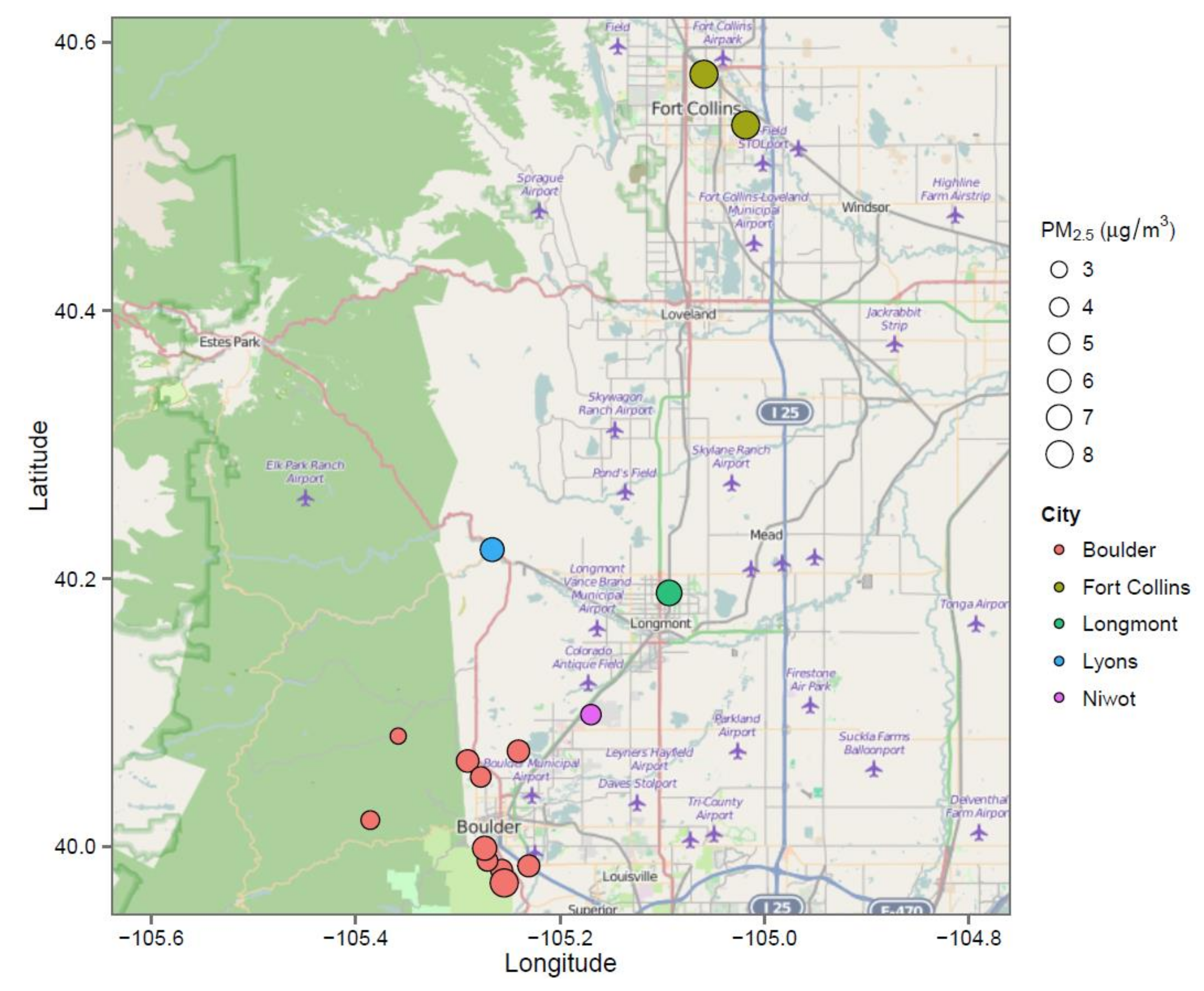
Fifteen households participated in this study. Homes were enrolled by verbal coordination and email with personal contacts of the research team. Criteria for inclusion were non-smoking occupants who had lived in the home for at least 2 years with two to five occupants, and a living space between 100–500 m2. All participants gave approval to participate in the study, in accordance with University of Colorado Boulder’s Institutional Review BoardProtocol # 12-0624. Study homes were located in five cities along the Front Range of Colorado (USA) within driving distance of Boulder (<two hours): Boulder (both in the city and mountains, 10 homes), Niwot, Longmont, and Lyons (one home in each), and Fort Collins (two homes). Figure 1 is a map of study homes labeled by the city in which the home resides, with coordinates jittered to maintain anonymity (map made in R, using the ggmap package [29]). Homes were assigned an alphabetical letter for identification purposes (A-R, skipping I, L, and O). A summary of household and occupant characteristics are presented in Table 1.
Eight home visits were scheduled for each home between 30 November 2012 and 4 December 2013. Seasonal splits for data analysis were determined by comparing meteorological seasons with the sampling schedule, resulting in the following dates defining “seasons” in this analysis: winter 30 November 2012–19 March 2013, spring 20 March 2013–20 June 2013, summer 21 June 2013–10 September 2013, and fall 11 November 2013–4 December 2013. Home D was only visited six times because major flooding occurred in the home after the sixth visit. Home M was visited three times during fall, resulting in nine total visits, and Home K was only visited once during winter, resulting in seven total visits.
2.2. Instrumentation and Metadata Collection
During each home visit, particulate matter (PM2.5 and PM10), total suspended particles (TSP) for microbial analysis, temperature (T), and relative humidity (RH) were monitored inside, and PM2.5, TSP, T and RH were monitored outside the home, for 24 h. Instruments were set up inside the home on a stand in the main living area. Outdoor instruments were installed in the backyard and were housed inside a weather-proof stand. Each resident filled out a web-based questionnaire to assess home characteristics, occupancy, cleaning product use, cleaning schedule, numbers of plants and animals, pesticide use, volunteer allergies and health conditions [30]. A walk-through inspection was also completed during every visit to document the physical attributes of the home (size, age, construction materials, general cleanliness, upholstered furniture, pets, plants, and ventilation). A time activity diary was filled out by residents during each 24-h sampling period, documenting activities that were classified as cooking, resuspension-inducing (cleaning, vigorous activity, vacuuming), fireplace use, increasing or using natural ventilation (opening bedroom, kitchen, or living room window, leaving the front or back door open, turning on the kitchen exhaust fan, or using an air filter in the bedroom, kitchen, or living room), occupying the kitchen, occupying rooms other than the kitchen, having 5 or more people at the house, or leaving the house unoccupied.
Three different methods were used to collect and measure particulate matter. Indoor and outdoor 24-h time-integrated mass concentrations of particle matter less than 2.5 μm in diameter (PM2.5) were measured by sampling at 20 L/min with a vacuum pump (Sensidyne Aircon 2, St. Petersburg, FL, USA) connected to a Harvard Impactor housing a 37-mm diameter Teflon filter (2-μm pore size, Pall CorporationR2PJ037, Port Washington, NY, USA). Gravimetric PM2.5 mass concentrations were determined by weighing Teflon filters before and after sampling in a temperature and RH-controlled weighing chamber according to well-established protocols [31]. Indoor PM10 concentrations were measured optically on a one-minute basis using a TSI Model 8530 DustTrak II Aerosol Monitor with an inlet flow rate of 3 L/min (sample flow rate of 2 L/min and sheath flow rate of 1 L/min, TSI, Shoreview, MN, USA). To summarize the seasonality of indoor PM10, average concentrations were calculated for each sampling day. DustTrak airflow was calibrated monthly. Total suspended particles were collected indoors and out by sampling onto nitrocellulose filters (4.15 cm in diameter, 0.45-μm pore size) for 24 h at 10 L/min with a vacuum pump (KNF Neuberger Inc., UN816.1.2 KTP Mini Diaphragm Vacuum Pump, Trenton, NJ, USA). DNA extraction from the TSP filters for sequencing and qPCR has been described elsewhere [32,33]. Temperature and relative humidity sensors (HOBO, Onset Corp., Cape Cod, MA, USA) were used to monitor indoors, outdoors, and inside the pump housings to check for overheating.
DustTrak (DT) data was reviewed weekly by the research team to note any unusual discrepancies; none were, however, found. Note that DustTrak 8530 mass concentrations are equivalent concentrations based on Arizona Road Dust tests, unless specific calibrations are undertaken to compare to the actual aerosol of interest. Therefore, direct comparison to other methods used to measure real outdoor or indoor aerosol made near and in homes may not be exact due to different optical properties [20,34,35]. The value of the DT measurements in our study was to have relative real-time concentrations that could be compared with the activity diaries. The DustTrak DRX’s 8533 and 8534 have been reported to exhibit sudden artifact jumps in concentration especially at low PM levels, but this behavior has not been reported for the DustTrak II 8530 that we used [36].
Table 2 shows the heating, ventilating, and air-conditioning characteristics along with potential pollutant sources in the homes. The ventilation potential score (VPS) (0–6) was based on questionnaire data and has been previously described and validated [37]. The VPS assessed the potential for adequate ventilation, assigning points for having at least one exterior window per room excluding bathrooms (1 point), a functional window or working exhaust fan for every bathroom (2 points), working exterior exhaust fans for all stoves (2 points), and additional exterior exhaust fans (1 point). Four study homes had a VPS equaling 3, which is considered less than adequate, and 11 homes had a VPS equal to or greater than four, which is adequate. During one visit for each home, a blower door test was conducted to measure air changes per hour when the house is depressurized to 50 Pascals (ACH50) (Minneapolis Blower Door, Model 3 Single Fan Unit, The Energy Conservatory, Minneapolis, MN, USA). ACH50 is a useful metric for comparing leakage of houses of different sizes [38]. Three homes had an ACH50 of less than or equal to 5, nine homes had an ACH50 between 5 and 10, and three homes had an ACH50 above 10. A house is considered tight when ACH50 is <3 for climate zones 3–8 (Colorado is 5–7) and 5 for climate zones 1–2 [39]. A tight house will have lower heating bills, fewer drafts but less infiltrating fresh air.
2.3. Data Analyses
Pearson’s correlation coefficient and linear regression were used to observe patterns between PM10, PM2.5, and PM2.5 indoor/outdoor (I/O) ratios. The nonparametric Kruskal–Wallis one-way analysis of variance (ANOVA) test was used to compare seasonal data. Nonparametric multiple comparison tests were assessed (two-sided Tukey contrast with the multivariate T-distribution asymptotic approximation method) after the Kruskal–Wallis ANOVA to determine which seasonal differences were statistically significant. Activity logs were assessed by calculating the total number of hours each activity was performed, referred to as activity-hours. The percent of total reported activity-hours for each activity by home was also calculated. The average relative reported activity-hours for each home is included in Figure S1.
To group homes showing similar seasonal variability and average concentrations, medoid clustering was performed using Euclidean distances for indoor PM10, indoor PM2.5, outdoor PM2.5, PM2.5 I/O ratios, indoor qPCR results, and outdoor qPCR results. Medoid clustering was performed using the Gower dissimilarity matrix for home characteristics, inhabitant characteristics, and HVAC system/emission source characteristics. Cluster number was determined iteratively by starting with fewer clusters (3–4) and increasing cluster number until meaningfulness of the resulting groupings diminished; individual time series often clustered by themselves when too many clusters were assessed. Agglomerative hierarchical clustering and principal component analysis aided in validating final cluster numbers.
3. Results and Discussion
3.1. Indoor and Outdoor Particulate Matter
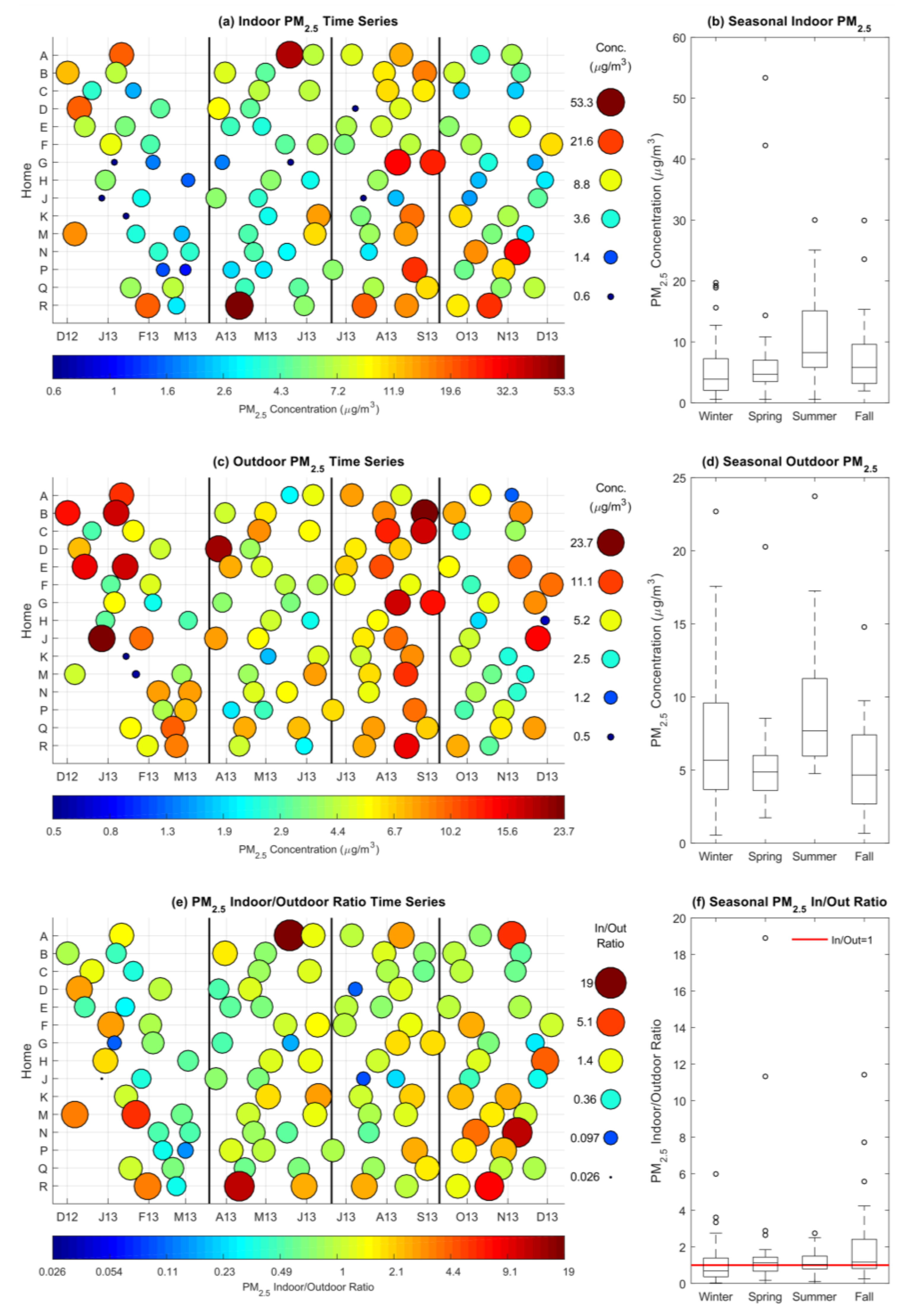
Indoor and outdoor PM2.5 concentrations of 24-h time-integrated samples and I/O ratios are presented in Figure 2a,c,e, respectively, where color and marker size represent PM concentration or I/O ratio. Box plots of seasonally grouped indoor and outdoor PM2.5 concentrations and I/O ratios are also shown in Figure 2b,d,f, respectively. Table S1 in the supplemental information presents overall and seasonal summary statistics for all measured PM concentrations. The average (±st. dev.) indoor and outdoor PM2.5 over the course of the year were 8.1 ± 8.1 μg/m3 and 6.8 ± 4.5 μg/m3, respectively. The average I/O ratio was higher than one, 1.6 ± 2.4, showing contributions from indoor sources. Table S2 contains summary statistics by home. These concentrations are 30% lower compared to a study of PM2.5 in Minneapolis, which reported yearly 24-h average PM2.5 indoor and outdoor concentrations of 10.9 ± 11.6 μg/m3 and 8.6 ± 6.6 μg/m3, respectively. The I/O ratio is comparable between the two studies [20]. In a study of PM2.5 in North Carolina, the concentrations were much higher compared to this study, measuring a mean indoor and outdoor concentration of 19.3 and 19.1 μg/m3 respectively [21].
The highest average PM2.5 concentrations occurred during summer both indoors (10.6 ± 7.4 μg/m3) and outdoors (9.2 ± 4.6 μg/m3). Outdoor PM2.5 was also higher during winter (7.5 ± 5.4 μg/m3) compared to spring and fall. The lowest seasonal average indoor PM2.5 value occurred during winter (6.1 ± 5.7 μg/m3). Indoor PM2.5 was statistically different during the summer compared to winter (p = 0.04) and spring (p = 0.02). Outdoor PM2.5 was statistically different during summer compared to fall (p = 0.0008) and spring (p = 0). Ramachadran et al. reports comparable levels to our study and also found higher indoor and outdoor PM2.5 in the summer and spring compared to fall, mainly due to open windows and doors [20]. Williams et al. did not find any seasonal differences, possibly due to the different climate conditions in North Carolina compared to Minnesota and Colorado, and measured levels that were twice as high as those measured in this study, 19 μg/m3 [21]. Urso et al. reports indoor PM1–2.5 levels of 3.1 and 4.1 μg/m3 during summer and winter, respectively, and much higher outdoor PM2.5 levels of 19.8 and 38.3 μg/m3 during summer and winter, respectively [16]. The PM2.5 levels measured in this study were low (and the Front Range typically has low PM2.5 concentrations). and below the USA’s Environmental Protection Agency current National Ambient Air Quality Standard of 35 μg/m3.
The seasonal average I/O ratio was lowest in the winter (1.2 ± 1.3) and summer (1.2 ± 0.7) and highest in the spring (2.0 ± 3.7) and fall (2.2 ± 2.5), but an analysis of variance (ANOVA) indicated no significant differences between seasons. These higher I/O ratios indicate either increased natural ventilation in study homes bringing more outdoor PM indoors or increased indoor emission events. I/O ratios above five occurred in every season and were observed to be mostly related to indoor cooking events (Figure 2): For example, Home A in May, Figure S8, and Home M in January, Figure S17. Very low I/O ratios (<0.3) also occurred and were due to elevated outdoor PM2.5 events or the home being unoccupied for much of the sampling period. Table S3 presents all seasonal hypothesis test results.
A linear regression of indoor versus outdoor PM2.5 concentrations showed no association (Figure 3a, R2 = 0.03), indicating that indoor PM2.5 was mainly due to sources in the homes. As shown in Figure 3b, Homes A (4.6 ± 6.5), N (2.6 ± 4.1), and R (3.8 ± 3.8) had the highest average I/O ratios. Home J had the lowest average I/O ratio (0.4 ± 0.3), likely due to the low indoor PM concentrations and elevated ambient PM2.5 concentrations measured at this home compared to other homes in Boulder (Figure 1). According to the random component superposition (RCS) model [40], the slope of the indoor-outdoor regression line provides an estimate of the fraction of the outdoor aerosol concentration that remains airborne in the home under equilibrium conditions, termed the infiltration factor, which for this study was 0.31 ± 0.17 (±st. error). The intercept is an estimate of the average contribution of indoor sources, which for this study was 5.97 ± 1.36 μg/m3. A parallel zero-intercept line to the regression line was drawn on Figure 3a, and if the assumptions of the RCS model are met, very few data points should reside below this line. This data set meets this assumption moderately well, as there are a few days where indoor PM2.5 levels were below the zero-intercept regression line.
The infiltration factor and the contribution from indoor sources estimated in this study are similar to those in previous studies. Wallace et al. [41] reported an average infiltration factor across six cities of 0.50 and an indoor source contribution of 6 μg/m3. The infiltration factor is a major variable determining the indoor-outdoor PM relationship and depends on the penetration coefficient, the air exchange rate, and the particle decay rate [42]. Ott et al. (reported an infiltration factor of 0.53 and an indoor source contribution of 18 μg/m3 [40]. Miller et al. reported for homes in Commerce City, CO (USA) an infiltration factor of 0.66 and an indoor source contribution of 21 μg/m3 [43]. Comparing the current study with the Commerce City study, the infiltration factor is more than two times higher in Commerce City homes, and the indoor source contribution is more than three times higher. This indicates the homes were leakier with many more indoor sources. The Commerce City study participants had much lower home ownership, higher home occupancy, fewer detached single-family homes, and lower VPS. The percentage of homes that were built before 1980 were similar for the two studies.
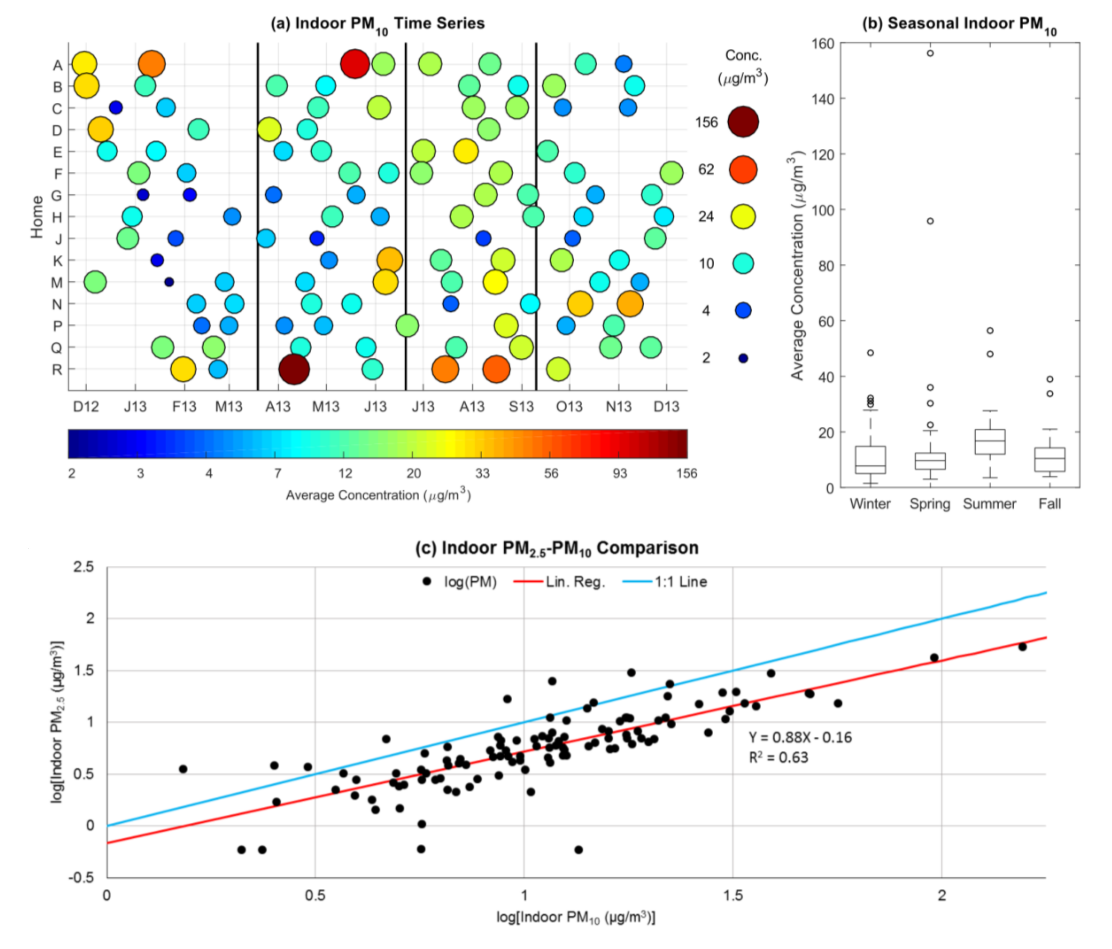
Figure 4a,b show the time series of average PM10 concentrations and seasonal boxplots of daily averages, respectively. The average (±st. dev.) PM10 concentration over the entire study was 15.4 ± 18.3 μg/m3. As was observed for indoor and outdoor PM2.5, the highest overall concentrations of PM10 occurred in the summer; two-way comparison tests showed summer indoor PM10 concentrations were significantly different from concentrations measured during all other seasons. Figure 4c shows the correlation observed between log-transformed indoor PM2.5 and indoor PM10 concentrations (Pearson’s correlation = 0.79, R2 = 0.63), indicating that changes in the fine fraction explain much of the variability in the larger size fraction. Some values in Figure 4c fall above the 1:1 line (PM2.5 > PM10), which may occur because we are comparing time-integrated filter-based PM2.5 measurements with averages of continuous optical-based PM10 measurements. Comparisons between these two measurement techniques are difficult, as both techniques have potential biases [44,45,46].
Statistical tests comparing PM concentrations and I/O ratio to ventilation characteristics were also conducted. No significant differences were observed between indoor PM2.5 or PM10 concentrations for homes with different ventilation potential scores (VPS). There were marginally significant differences (p = 0.10) in average I/O ratios between homes with VPS of six (2.8 ± 4.6, n = 15), five (I/O ratios of 1.7 ± 19, n = 54), and homes with a VPS of three, (1.0 ± 0.7, n = 31). No linear trends were observed between ACH50 and pollutant concentrations.
3.2. Indoor and Outdoor qPCR
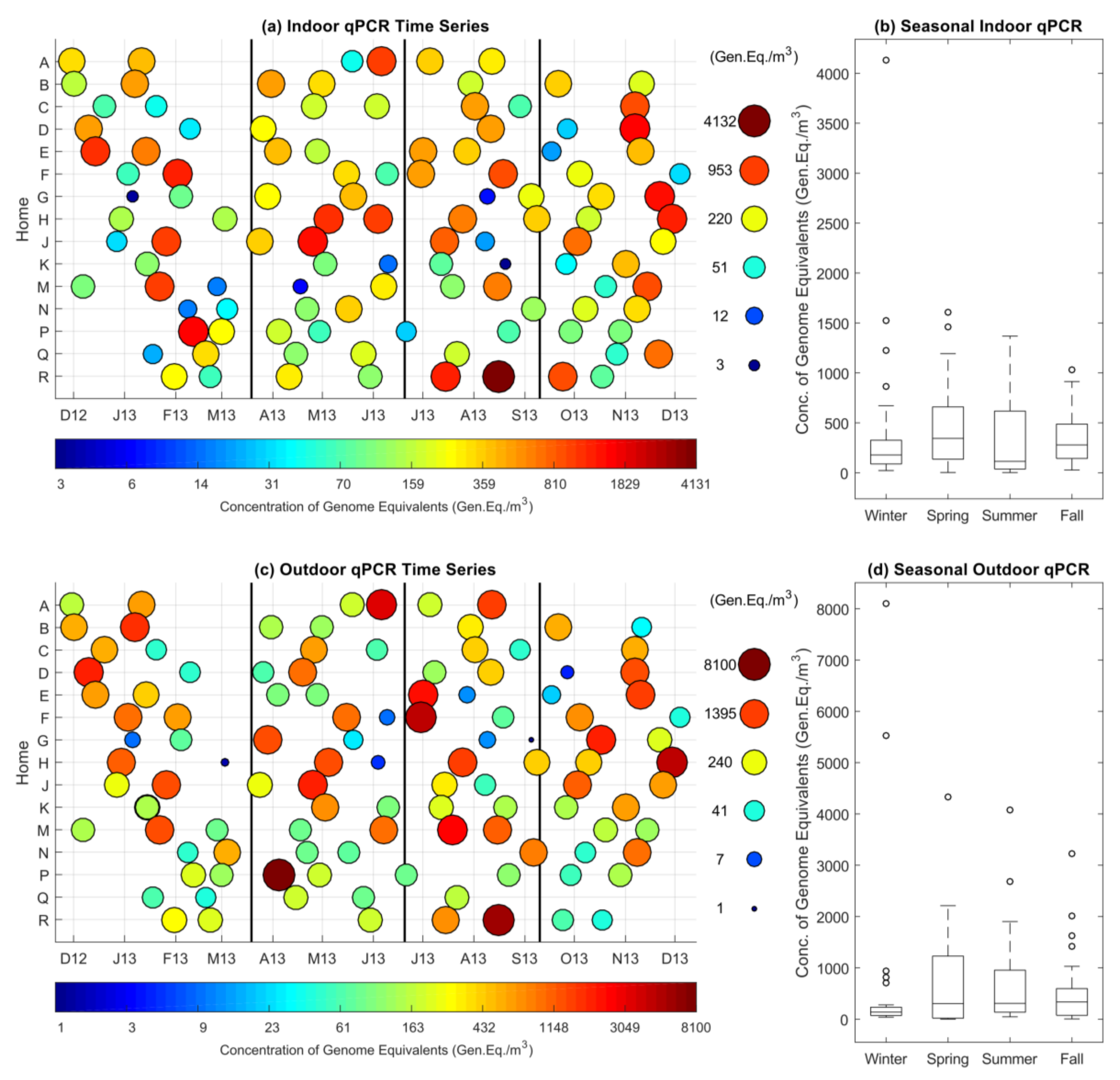
Indoor and outdoor bacterial biomass concentrations of 24-h time-integrated samples are presented in Figure 5a,c, where color and marker size represent genome equivalent copy numbers (gen eq)/m3. Our results are reported in E. coli genome equivalents, but they can be interpreted as estimates of the total number of bacterial cells per sample. As indicated in a previous study using the same qPCR methods, these results are useful for relative microbial abundance comparisons within a study, but the values should not be interpreted to represent absolute cell concentrations [32,33]. Box plots of seasonally grouped indoor and outdoor bacterial biomass concentrations are shown in Figure 5b,d. There was no seasonal variability in the time series of qPCR data, based on Kruskal–Wallis ANOVA test. Outdoor levels (average 675 ± 1158 gen eq/m3) were generally higher than indoor levels (average 391 ± 522 gen eq/m3). This result is similar to the results from a residential Berkeley, CA (USA) study, which showed bacterial biomass was higher outdoors than indoors [23], but is opposite a study of a Berkeley, CA classroom that showed indoors higher than outdoors [26]. A linear regression of indoor versus outdoor qPCR concentrations showed limited association (R2 = 0.20).
The qPCR I/O ratios varied by season with spring being the highest (p-value = 0.006). Winter, spring, summer and fall average I/O ratios were 1.6 ± 1.8, 18 ± 46, 0.71 ± 1.3, and 2.3 ± 3.3, respectively. Multiple comparison tests showed that the summer I/O ratios were statistically significantly lower than all other seasons (Su/W p = 0.006; Su/Sp p = 0.03; and Su/F p = 0.03). We saw no indoor-outdoor correlation for the entire data set, but there were significant correlations when the data were split according to season, with the strongest in fall (Pearson’s Corr = 0.66) and summer (Pearson’s Corr = 0.63), followed by winter (Pearson’s Corr = 0.26) then spring (Pearson’s Corr = 0.16).
Emerson et al. is a companion paper to this study and reported that the indoor air bacterial community composition was significantly different between homes and within each home over time [33]. Indoor air bacterial communities from the same home were often just as different at adjacent time points as they were across larger temporal distances. Temporal variation correlated with temperature and relative humidity. Individual taxa that were significantly more abundant in indoor, relative to outdoor, air included Pasteurellales, which has been shown to be associated with cats and dogs in indoor environments. Interestingly, none of the environmental variables (i.e., those described in this paper including PM2.5, PM10) were correlated with the indoor air microbial community composition.
3.3. Clustering
The primary goal of the data clustering analysis, which is a common exploratory data mining technique, was to place homes into groups suggested by the data, such that the homes in a given cluster tend to have similar pollutant concentrations, physical attributes, inhabitant characteristics, or HVAC system configuration. This analysis was undertaken to identify common characteristics that explain the data. Details of the clustering results are described in the Supplemental Information. Table S4 contains a summary of categorical home characteristic results. Homes tended to cluster depending on whether there were children in the home, leakage area, size of the home, location, and fireplace/furnace/air conditioning (AC) type. These data agree with previous studies of home characteristics and healthy indoor air quality, e.g., [16,19]. Emerson et al. found that similar categorical home characteristics were significantly correlated with the indoor air microbial community composition in these same study homes, including presence of one or more dogs, how long the family had lived at the residence, fireplace/furnace/AC type, and whether or not the HVAC system used electrostatic filters [33]. Table S5 details the clustering results for all pollutant time series. Time series for clustering were based on sample number as shown in the time series of clusters (Figures S2–S7) for indoor and outdoor PM2.5, PM2.5 I/O ratio, indoor PM10 and indoor and outdoor qPCR data. Indoor PM2.5 and PM10 clusters identified homes with similar elevated concentrations from cooking and infiltration of summertime outdoor pollution. Outdoor PM2.5 clusters substantiated the results that outdoor particle concentrations varied spatially and depended on location. Clusters from I/O ratios identified homes with common characteristics that lead to elevated ratios.
3.4. Activity Journals and Indoor PM10
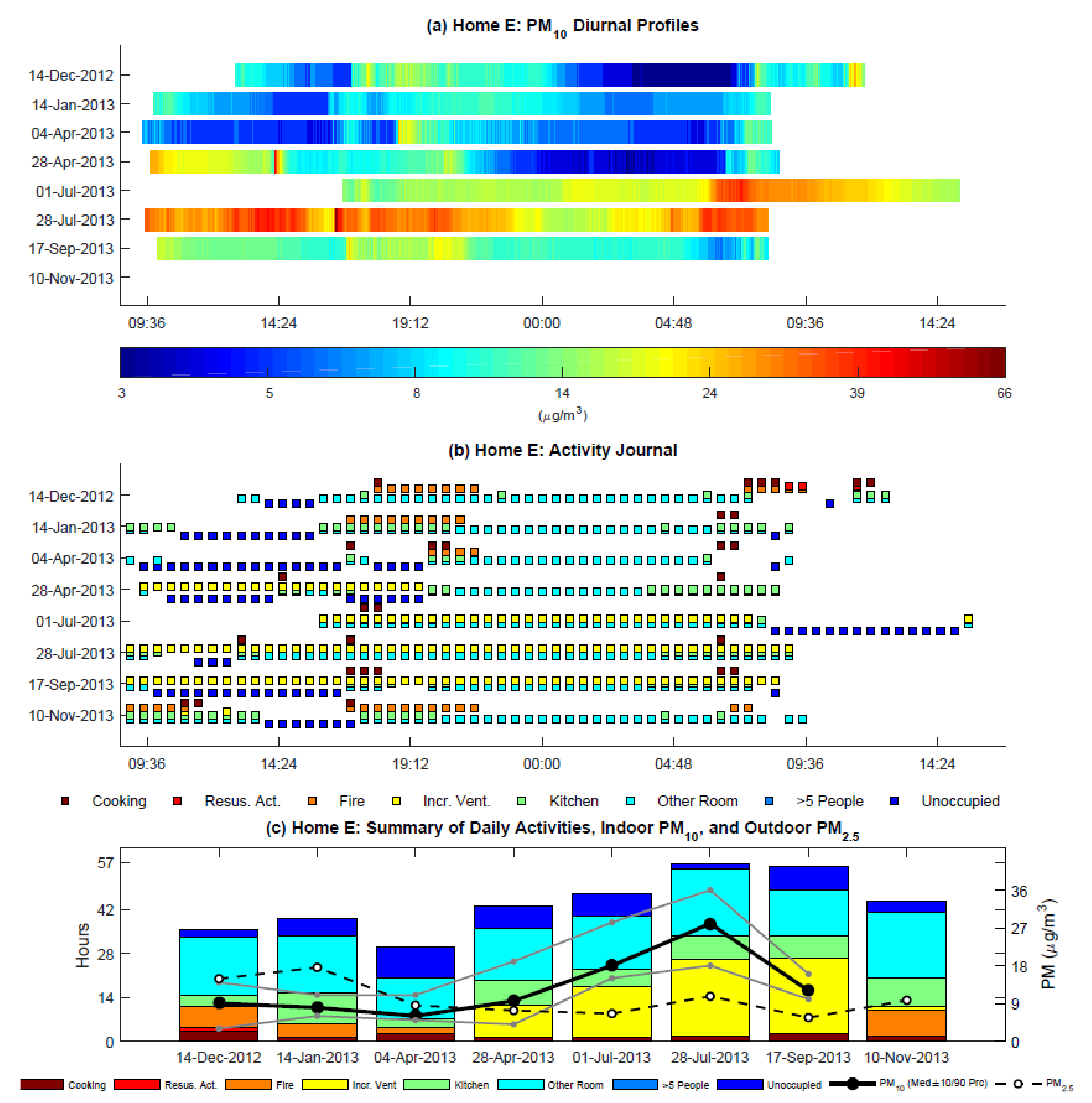
Relationships between occupant activities and one-minute indoor PM10 concentrations were explored. Figure 6 shows the two data sets plotted together for home E. Plots for all other homes are included in the supplemental information (Figures S8–S21). These figures show the complex interplay between occupant activities, home ventilation conditions, indoor particulate matter emissions, and outdoor pollutant infiltration, the combination of which helps to explain the clustering trends observed for daily PM10 means. Completeness of the activity logs varied between homes, and comparisons between activity logs and pollutant concentrations for some homes were limited due to low activity log response rates. The average time spent on each activity relative to the total reported activity-hours by home is presented in Figure S1.
Cooking frequently elevated PM10 concentrations at night and in the mornings when dinner and breakfast were prepared (Figure 6a, 14 December 2012), though not all cooking events were accompanied by increased PM10 concentrations. This is likely because only some cooking activities (using the stove or oven) produce particulate emissions [5].
PM10 concentrations often decreased overnight when occupants were asleep and whenever the home was unoccupied (Figure 6a, 28 April 2013). Sometimes peaks were observed when resuspension activities were reported, but resuspension-caused peaks were much lower than peak concentrations for cooking events (Figure 6a, 14 December 2012).
Most events classified as increased ventilation involved opening windows or doors. The indoor PM10 response to this activity depended on outdoor aerosol concentrations, estimated with the outdoor PM2.5 filter samples. Infiltration of poor outdoor air combined with cooking events increased indoor PM10 concentrations for many homes that increased their ventilation during summer and winter (Figure 6c, 28 July 2013). Increasing ventilation during cooking events was observed to often shorten the residence time of the emitted particles, unless outdoor aerosol concentrations were elevated.
The two days with the highest PM10 values occurred at home A on 19 May 2013 (Figure S8), reaching about 850 µg/m3, and at home R on 11 April 2013 (Figure S21), reaching about 3000 µg/m3. These two days correspond to days with similarly high indoor PM2.5, but not necessarily elevated outdoor PM2.5. These days are cases of cooking emissions and poor ventilation leading to unhealthy concentrations of indoor aerosols. Home A is also interesting because PM10 decayed very slowly over night during the first three sampling days in Nov, Jan and May. This is likely because the home had an oversized forced-air heating unit and no air-conditioning that mixed the PM10 efficiently through the entire house, and no actions were taken to increase natural ventilation. The cooking event at home R on 11 April 2013 (Figure S21) can be attributed to burning pancakes and an inability to exhaust the smoke, as there was no exhaust hood over the stove.
As a result of the extremely high PM levels observed in home R and the adverse health impacts (asthma symptoms, respiratory infections) reported by the residents upon moving into this home, further investigation was warranted. Home R was weatherized, heated with radiant heating from flooring, and was cooled by a swamp cooler in the summer with no forced-air ventilation. It had the lowest ACH50 of all our study homes (4 1/h). At the conclusion of our study, we suggested the family install a ventilation system in their home to increase their outdoor air exchange rates. An energy recovery ventilation (ERV) system was added to the home. This system was designed to always bring some outside air into the home. Since the installation, the homeowners noticed their health significantly improved and they were able to stop using their asthma inhalers during the winter. At the request of the homeowners, a follow up assessment was performed March 2015 to determine the impact of the ERV system on the indoor air quality in the home. The TSI DustTrak that was used in the previous study was no longer available for the follow-up study; therefore, a Dylos Pro1100 (Riverside, CA, USA) was used to measure particulate matter counts. The small particle counts were converted to PM2.5 mass concentrations using the calibration curve determined by Klepeis et al. [47]. The average PM2.5 concentration during the 2015 sampling was 4.7 µg/m3, which is much lower than the average PM2.5 concentration of 18.7 µg/m3 found in the 2013 study.
Studies such as this one that occur over the course of the year in a small number of homes will capture outlier activities and events that drive indoor air quality. For example, in home N, during the fall season on 8 October and 9 November 2013 flood remediation activities took place and drove the PM10 concentrations higher. In home R, pancakes were burned on 11 April 2013, resulting in severely elevated PM10 concentrations. On the other end of the scale, there were many sampling days in which no one was home and the PM10 levels were very low. Because cooking with a stove or oven has such a significant impact on indoor PM2.5, collecting more information about what was cooked and the appliances used would be useful in future long-term residential air quality studies. In future long-term home indoor air quality studies, it would be useful to control for many of the home characteristics to limit the possible covariates in cross-home statistical comparisons between IAQ and building design factors.
4. Conclusions
The results of this study show that indoor particulate concentrations in homes and outside of homes around Boulder, Colorado vary seasonally with highest levels in summer. The climate in this area is classified as semi-arid, climate zone number 5 [48], which has a strong seasonal component to temperature and relative humidity and results in closed-up homes with heating activities in the winter, and more natural ventilation and/or air-conditioning in the summer.
Indoor pollutant concentrations were observed to be highly dependent on occupant cooking, use of natural ventilation, and outdoor air conditions. Little variability in indoor pollutant data can be explained by home characteristic attributes alone. Strong impacts of home location could also be seen in the data. Results also support the conclusion that most residential indoor PM10 is actually PM2.5 and is from either indoor cooking or outdoor PM2.5.
Clustering analysis revealed that home characteristics were more directly related to indoor PM2.5 levels, including type of heating and air-conditioning, stove type, ACH50, and home size. Location of the home was more directly related to outdoor PM2.5, with northern front range locations experiencing higher PM2.5. Home A and R were typically separated from all clusters, due to their very distinct ventilation characteristics. Home R had the highest indoor PM2.5, elevated I/O ratio, high indoor PM10. This home had no furnace, used radiative floor heating, evaporative cooling and had an ACH50 of 4.2 (lowest in our sample). Home A had an oversized furnace for the home and a high ACH50 of 11.8. Home B and E also regularly clustered together and they were both Fort Collins homes. Home Q also separated by itself with the highest indoor qPCR and the highest ACH50.
Implications of this work are that while we saw very little seasonal variability in the indoor air bacterial community composition in these homes (companion paper Emerson et al. [33]) and no relationship between microbial community composition and airborne particulate matter, we did see strong seasonal variability in the airborne particulate matter in and outside of the study homes. Thus, when outdoor PM2.5 concentrations are elevated such as in the summer, indoor exposures can be reduced by keeping windows closed, using air-conditioning, or in-home filtration. Cooking often elevated indoor air particulate concentrations, suggesting exposures could be reduced by using stove exhaust hoods continuously while cooking and in-home filtration. The impact of home characteristics could be seen both in the microbial community composition and particulate matter data, although with a larger sample size of homes, a clearer relationship would be better elucidated. For example, our study showed that home HVAC design impacts indoor PM2.5 concentrations, suggesting residential exposure could be mitigated through good design, sizing systems correctly, and even using an ERV system to bring in fresh air. Home leakage as measured by ACH50 was also another impactful characteristic both on microbial communities and particle levels. Tighter homes both keep out outdoor air pollution and keep in indoor air pollution. A move towards home designs with outdoor air filtered and supplied with ERVs would allow for much tighter building construction while maintaining healthy indoor particle levels, as long as cooking emissions were ventilated.
Supplementary Materials
The following are available online at https://www.mdpi.com/2073-4433/9/4/133/s1.
Acknowledgments
We are deeply grateful to all of the study participants who generously shared their time and homes. We thank the students who supported this project: Oluwaseun Oyatogun, Kangqian Wu, Suraj Prabhu, Allie James, Megan Bangert, and Amanda Bradbury. This study was funded by grants awarded to Nicholas Clements and Shelly L. Miller from the Alfred P. Sloan Foundation. Publication of this article was funded by the University of Colorado Boulder Libraries Open Access Fund.
Author Contributions
S.L.M. and N.F. conceived and designed the experiments; P.K. and J.B.E performed the experiments; N.C., J.B.M., and P.K. analyzed the data; S.L.M., P.K., and N.C. wrote the paper.
Conflicts of Interest
The authors declare no conflict of interest.
References
- Dales, R.; Liu, L.; Wheeler, A.J.; Gilbert, N.L. Quality of indoor residential air and health. CMAJ 2008, 179, 147–152. [Google Scholar] [CrossRef] [PubMed]
- Chan, W.R.; Logue, J.M.; Wu, X.; Klepeis, N.E.; Fisk, W.J.; Noris, F.; Singer, B.C. Quantifying fine particle emission events from time-resolved measurements: Method description and application to 18 California low-income apartments. Indoor Air 2018, 28, 89–101. [Google Scholar] [CrossRef] [PubMed]
- Chen, C.; Zhao, B. Review of relationship between indoor and outdoor particles: I/O ratio, infiltration factor and penetration factor. Atmos. Environ. 2011, 45, 275–288. [Google Scholar] [CrossRef]
- Buonanno, G.; Morawska, L.; Stabile, L. Particle emission factors during cooking activities. Atmos. Environ. 2009, 43, 3235–3242. [Google Scholar] [CrossRef] [Green Version]
- Abdullahi, K.; Delgado-Saborit, J.; Harrison, R.M. Emissions and indoor concentrations of particulate matter and its specific chemical components from cooking: A review. Atmos. Environ. 2013, 71, 260–294. [Google Scholar] [CrossRef]
- Jones, N.C.; Thornton, C.A.; Mark, D.; Harrison, R.M. Indoor/outdoor relationships of particulate matter in domestic homes with roadside, urban, and rural locations. Atmos. Environ. 2000, 34, 2603–2612. [Google Scholar] [CrossRef]
- He, C.; Morawska, L.; Hitchins, J.; Gilbert, D. Contribution from indoor sources to particle number and mass concentrations in residential houses. Atmos. Environ. 2004, 38, 3405–3415. [Google Scholar] [CrossRef] [Green Version]
- Olson, D.A.; Burke, J.M. Distributions of PM2.5 Source Strengths for Cooking from the Research Triangle Park Particulate Matter Panel Study. Environ. Sci. Technol. 2006, 40, 163–169. [Google Scholar] [CrossRef] [PubMed]
- Knibbs, L.D.; He, C.; Duchaine, C.; Morawska, L. Vacuum Cleaner Emissions as a Source of Indoor Exposure to Airborne Particles and Bacteria. Environ. Sci. Technol. 2011, 46, 534–542. [Google Scholar] [CrossRef] [PubMed]
- Ferro, A.R.; Kopperud, R.J.; Hildemann, L.M. Source Strengths for Indoor Human Activities that Resuspend Particulate Matter. Environ. Sci. Technol. 2004, 38, 1759–1764. [Google Scholar] [CrossRef] [PubMed]
- Serfozo, N.; Chatoutsidou, S.E.; Lazaridis, M. The effect of particle resuspension during walking activity to PM10 mass and number concentrations in an indoor microenvironment. Build. Environ. 2014, 82, 180–189. [Google Scholar] [CrossRef]
- Larson, T.; Gould, T.; Simpson, C.; Liu, L.-J.S.; Claiborn, C.; Lewtas, J. Source Apportionment of Indoor, Outdoor, and Personal PM2.5 in Seattle, Washington, Using Positive Matrix Factorization. Indoor Air 2004, 54, 1175–1187. [Google Scholar] [CrossRef]
- Bari, Md.A.; Kindzierski, W.B.; Wallace, L.A.; Wheeler, A.J.; MacNeill, M.; Heroux, M.-E. Indoor and Outdoor Levels and Sources of Submicron Particles (PM1) at Homes in Edmonton, Canada. Environ. Sci. Technol. 2015, 49, 6419–6429. [Google Scholar] [CrossRef] [PubMed]
- Perrino, C.; Tofful, L.; Canepari, S. Chemical characterization of indoor and outdoor fine particulate matter in an occupied apartment in Rome, Italy. Indoor Air 2015. [Google Scholar] [CrossRef] [PubMed]
- Lim, M.T.; Phan, A.; Roddy, D.; Harvey, A. Technologies for measurement and mitigation of particulate emissions from domestic combustion of biomass: A review. Renew. Sustain. Energy Rev. 2015, 49, 574–584. [Google Scholar] [CrossRef]
- Urso, P.; Cattaneo, A.; Garramone, G.; Peruzzo, C.; Cavallo, D.M.; Carrer, P. Identification of particulate matter determinants in residential homes. Build. Environ. 2015, 86, 61–69. [Google Scholar] [CrossRef]
- Meng, Q.Y.; Spector, D.; Colome, S.; Turpin, B. Determinants of indoor and personal exposure to PM2.5 of indoor and outdoor origin during the RIOPA study. Atmos. Environ. 2009, 43, 5750–5758. [Google Scholar] [CrossRef] [PubMed]
- Klepeis, N.E.; Bellettiere, J.; Hughes, S.C.; Nguyen, B.; Berardi, V.; Liles, S.; Obayashi, S.; Hofstetter, C.R.; Blumberg, E.; Hovell, M.F. Fine particles in homes of predominantly low-income families with children and smokers: Key physical and behavioral determinants to inform indoor-air-quality interventions. PLoS ONE 2017, 12, e0177718. [Google Scholar] [CrossRef] [PubMed]
- Richardson, G.; Eick, S.A.; Shaw, S.R. Designing a Simple Tool Kit and Protocol for the Investigation of the Indoor Environment in Homes. Indoor Built Environ. 2006, 15, 411–424. [Google Scholar] [CrossRef]
- Ramachandran, G.; Adgate, J.L.; Pratt, G.C.; Sexton, K. Characterizing Indoor and Outdoor 15 Minute Average PM2.5 Concentrations in Urban Neighborhoods. Aerosol Sci. Technol. 2003, 37, 33–45. [Google Scholar] [CrossRef]
- Williams, R.; Suggs, J.; Rea, A.; Leovic, K.; Vette, A.; Croghan, C.; Sheldon, L.; Rodes, C.; Thornburg, J.; Ejire, A.; et al. The Research Triangle Park particulate matter panel study: PM mass concentration relationships. Atmos. Environ. 2003, 37, 5349–5364. [Google Scholar] [CrossRef]
- Jaenicke, R. Abundance of Cellular Material and Proteins in the Atmosphere. Science 2005, 308, 73. [Google Scholar] [CrossRef] [PubMed]
- Adams, R.I.; Miletto, M.; Lindow, S.E.; Taylor, J.W.; Bruns, T.D. Airborne Bacterial Communities in Residences: Similarities and Differences with Fungi. PLoS ONE 2014, 9, e91283. [Google Scholar] [CrossRef] [PubMed]
- Qian, J.; Hospodsky, D.; Yamamoto, N.; Nazaroff, W.W.; Peccia, J. Size-resolved emission rates of airborne bacteria and fungi in an occupied classroom. Indoor Air 2012, 22, 339–351. [Google Scholar] [CrossRef] [PubMed]
- Burge, H. Bioaerosols: Prevalence and health effects in the indoor environment. J. Allergy Clin. Immunol. 1990, 86, 687–701. [Google Scholar] [CrossRef]
- Hospodsky, D.; Qian, J.; Nazaroff, W.W.; Yamamoto, N.; Bibby, K.; Rismani-Yazdi, H.; Peccia, J. Human Occupancy as a Source of Indoor Airborne Bacteria. PLoS ONE 2012, 7, e34867. [Google Scholar] [CrossRef] [PubMed] [Green Version]
- Torvinen, E.; Torkko, P.; Rintala, A.N.H. Real-time PCR detection of environmental mycobacteria in house dust. J. Microbiol. Methods 2010, 82, 78–84. [Google Scholar] [CrossRef] [PubMed]
- Kaarakainen, P.; Meklin, T.; Hyvärinen, A.; Kärkkäinen, P.; Vepsäläinen, A.; Hirvonen, M.-R.; Nevalainen, A. Seasonal variation in airborne microbial concentrations and diversity at landfill, urban and rural sites. CLEAN–Soil Air Water 2008, 36, 556–563. [Google Scholar] [CrossRef]
- Kahle, D.; Wickham, H. ggmap: Spatial Visualization with ggplot2. R J. 2013, 5, 144–161. [Google Scholar]
- Barberán, A.; Dunn, R.R.; Reich, B.J.; Pacifici, K.; Laber, E.B.; Menninger, H.L.; Morton, J.M.; Henley, J.B.; Leff, J.W.; Miller, S.L.; et al. The ecology of microscopic life in household dust. Proc. R. Soc. B 2015, 282, 20151139. [Google Scholar] [CrossRef] [PubMed]
- Dutton, S.J.; Schauer, J.J.; Vedal, S.; Hannigan, M.P. PM 2.5 characterization for time series studies: Pointwise uncertainty estimation and bulk speciation methods applied in Denver. Atmos. Environ. 2009, 43, 1136–1146. [Google Scholar] [CrossRef] [PubMed]
- Emerson, J.B.; Keady, P.B.; Brewer, T.E.; Clements, N.; Morgan, E.E.; Awerbuch, J.; Miller, S.L.; Fierer, N. Impacts of Flood Damage on Airborne Bacteria and Fungi in Homes after the 2013 Colorado Front Range Flood. Environ. Sci. Technol. 2015, 49, 2675–2684. [Google Scholar] [CrossRef] [PubMed]
- Emerson, J.B.; Keady, P.B.; Clements, N.; Morgan, E.E.; Awerbuch, J.; Miller, S.L.; Fierer, N. High temporal variability in airborne bacterial diversity and abundance inside single-family residences. Indoor Air 2017, 27, 576–586. [Google Scholar] [CrossRef] [PubMed]
- McNamara, M.L.; Noonan, C.W.; Ward, T.J. Correction factor for continuous monitoring of wood smoke fine particulate matter. Aerosol Air Qual. Res. 2011, 11, 315–322. [Google Scholar] [CrossRef] [PubMed]
- Spinazzè, A.; Fanti, G.; Borghi, F.; Del Buono, L.; Campagnolo, D.; Rovelli, S.; Cattaneo, A.; Cavallo, D.M. Field comparison of instruments for exposure assessment of airborne ultrafine particles and particulate matter. Atmos. Environ. 2017, 154, 274–284. [Google Scholar] [CrossRef]
- Rivas, I.; Mazaheri, M.; Viana, M.; Moreno, T.; Clifford, S.; He, C.; Bischof, O.F.; Martins, V.; Reche, C.; Alastuey, A.; et al. Identification of technical problems affecting performance of DustTrak DRX aerosol monitors. Sci. Total Environ. 2017, 584, 849–855. [Google Scholar] [CrossRef] [PubMed]
- Litt, J.S.; Goss, C.; Diao, L.; Allshouse, A.; Diaz-Castillo, S.; Barwell, R.A.; Hendrikson, E.; Miller, S.L.; DiGuiseppi, C. Housing Environments and Child Health Conditions Among Recent Mexican Immigrant Families: A Population-Based Study. J. Immigr. Minor. Health 2010, 12, 617–625. [Google Scholar] [CrossRef] [PubMed]
- Hancock, E.; Norton, P.; Hendron, B. Building America System Performance Test Practices: Part 2, Air-Exchange Measurements; NREL/TP-550-30270; National Renewable Energy Laboratory: Golden, CO, USA, 2002; p. 2. [Google Scholar]
- IECC. International Energy Conservation Code. Building Technologies Program Air Leakage Guide, Report PNNL-SA-82900. 2012. Available online: https://www.energycodes.gov/sites/default/files/documents/BECP_Buidling%20Energy%20Code%20Resource%20Guide%20Air%20Leakage%20Guide_Sept2011_v00_lores.pdf (accessed on 10 January 2018).
- Ott, W.; Wallace, L.; Mage, D. Predicting particulate (PM10) personal exposure distributions using a random component superposition statistical model. Air Waste Manag. Assoc. 2000, 50, 1390–1406. [Google Scholar] [CrossRef]
- Wallace, L.A.; Mitchell, H.; O’Connor, G.T.; Neas, L.; Lippmann, M.; Kattan, M.; Koenig, J.; Stout, J.W.; Vaughn, B.J.; Wallace, D.; et al. Particle concentrations in inner-city homes of children with asthma: The effect of smoking, cooking, and outdoor pollution. Environ. Health Perspect. 2003, 111, 1265–1272. [Google Scholar] [CrossRef] [PubMed]
- Wallace, W.; Williams, R. Use of personal-indoor-outdoor sulfur concentrations to estimate the infiltration factor and outdoor exposure factor for individual homes and persons. Environ. Sci. Technol. 2005, 39, 1707–1714. [Google Scholar] [CrossRef] [PubMed]
- Miller, S.L.; Scaramella, P.; Campe, J.; Goss, C.W.; Diaz-Castillo, S.; Hendrikson, E.; DiGuiseppi, C.; Litt, J. An assessment of indoor air quality in recent Mexican immigrant housing in Commerce City, Colorado. Atmos. Environ. 2009, 43, 5661–5667. [Google Scholar] [CrossRef]
- Yanosky, J.D.; Williams, P.L.; MacIntosh, D.L. A comparison of two direct-reading aerosol monitors with the federal reference method for PM2.5 in indoor air. Atmos. Environ. 2002, 36, 107–113. [Google Scholar] [CrossRef]
- Kim, J.Y.; Magari, S.R.; Herrick, R.F.; Smith, T.J.; Christiani, D.C. Comparison of Fine Particle Measurements from a Direct-Reading Instrument and a Gravimetric Sampling Method. J. Occup. Environ. Hyg. 2004, 1, 707–715. [Google Scholar] [CrossRef] [PubMed]
- Moya, M.; Madronich, S.; Retama, A.; Weber, R.; Baumann, K.; Nenes, A.; Castillejos, M.; Ponce de Leon, C. Identification of chemistry-dependent artifacts on gravimetric PM fine readings at the T1 site during the MILAGRO field campaign. Atmos. Environ. 2011, 45, 244–252. [Google Scholar] [CrossRef]
- Klepeis, N.E.; Hughes, S.C.; Edwards, R.D.; Allen, T.; Johnson, M.; Chowdhury, Z.; Smith, K.R.; Boman-Davis, M.; Bellettiere, J.; Hovell, M.F. Promoting smoke-free homes: A novel behavioral intervention using real-time audio-visual feedback on airborne particle levels. PLoS ONE 2013, 8, e73251. [Google Scholar] [CrossRef] [PubMed]
- ASHRAE 169-2006. Standard for Weather Data for Building Design Standards Created by American Society of Heating, Refrigerating and Air-Conditioning Engineers; ASHRAE: Atlanta, GA, USA; Available online: https://www.ashrae.org/resources--publications/bookstore/climate-data-center#std169 (accessed on 10 January 2018).
Figure 1.
Study homes in the Front Range of Colorado (marker size represents median outdoor particulate matter (PM)2.5 in µg/m3 measured at each home, ©OpenStreetMap contributors).
Figure 1.
Study homes in the Front Range of Colorado (marker size represents median outdoor particulate matter (PM)2.5 in µg/m3 measured at each home, ©OpenStreetMap contributors).

Figure 2.
(a) Indoor PM2.5 concentrations; (b) box plots of seasonal indoor PM2.5 concentrations; (c) outdoor PM2.5 concentrations; (d) box plots of seasonal outdoor PM2.5 concentrations; (e) PM2.5 indoor/outdoor ratios; and (f) seasonal box plots of PM2.5 indoor/outdoor ratios (in (a,c,e) color and marker size are scaled logarithmically and indicate pollutant values; vertical bars separate seasons).

Figure 3.
(a) Scatterplot of indoor vs. outdoor PM2.5 mass concentrations and linear regression (dashed line is the regression line with the intercept removed); and (b) bar plot of mean (±SD) PM2.5 indoor/outdoor ratios per house. The bar color for each home in (b) corresponds to the marker color in (a).
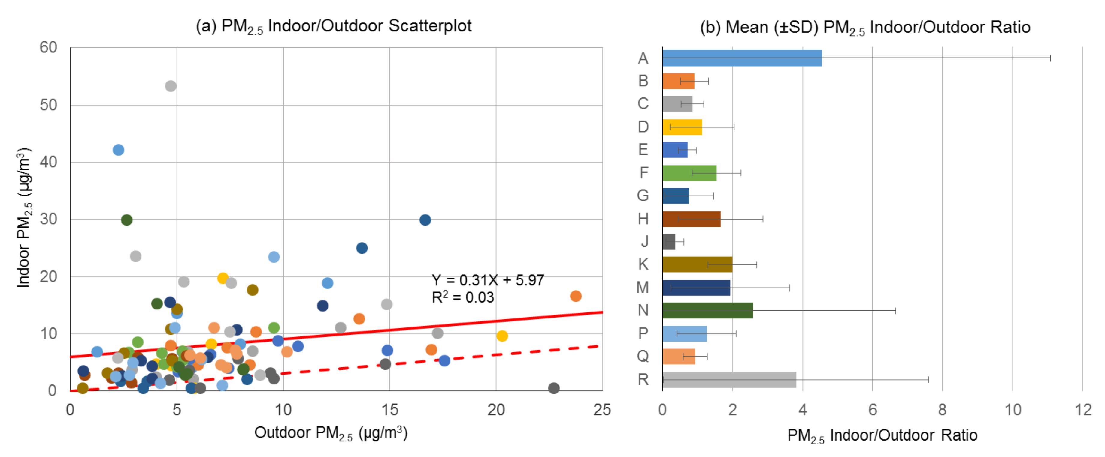
Figure 4.
(a) Average indoor PM10 concentrations (color and marker size are on a logarithmic scale and indicate PM10 concentrations; vertical bars separate seasons); (b) seasonal box plots of average indoor PM10 concentrations; and (c) scatter plot and linear regression between indoor PM10 and PM2.5 concentrations.

Figure 5.
(a) Indoor qPCR concentrations; (b) seasonal box plots of indoor qPCR concentrations; (c) outdoor qPCR concentrations; and (d) seasonal box plots of outdoor qPCR concentrations (color and marker size are on a logarithmic scale and indicate qPCR concentrations; vertical bars separate seasons).

Figure 6.
(a) Indoor PM10 diurnal profiles; (b) activity journal on half-hour intervals; and (c) summed activity-hours per day, indoor PM10, and outdoor PM2.5 concentrations for Home E.
Figure 6.
(a) Indoor PM10 diurnal profiles; (b) activity journal on half-hour intervals; and (c) summed activity-hours per day, indoor PM10, and outdoor PM2.5 concentrations for Home E.


Table 1.
Physical attributes and inhabitant characteristics of study homes.
| Home | Location | Year Built | Time in Home (Years) | Surface Area (m2) | Volume (m3) | Basement/Garage | # Residents | # Kids | #Male | # Female |
|---|---|---|---|---|---|---|---|---|---|---|
| A | Boulder city 1 | 1965 | 2–5 | 167.4 | 333.9 | Yes/Yes | 3 | 1 | 1 | 2 |
| B | Fort Collins 1 | 1995 | 6–10 | 347.2 | 1011.1 | Yes/Yes | 3 | 1 | 1 | 2 |
| C | Boulder city 1 | 1999 | 6–10 | 318.5 | 885.1 | Yes/Yes | 4 | 2 | 2 | 2 |
| D | Lyons 1 | 1970 | 6–10 | 129.9 | 326.5 | No/Yes | 3 | 1 | 1 | 2 |
| E | Fort Collins 1 | 1965 | 6–10 | 278.1 | 663.4 | Yes/Yes | 4 | 2 | 2 | 2 |
| F | Boulder city 1 | 1985 | 6–10 | 279.6 | 765.4 | Yes/Yes | 3 to 5 | 1 to 3 | 1 to 2 | 2 to 3 |
| G | Boulder city 1 | 1986 | 11–20 | 465.7 | 1208.2 | Yes/Yes | 2 | 0 | 1 | 1 |
| H | Boulder mountain 2 | 1985 | >20 | 114.5 | 276.5 | No/No | 2 | 0 | 1 | 1 |
| J | Boulder city 1 | 1968 | >20 | 229 | 517.7 | Yes/Yes | 3 | 0 | 2 | 1 |
| K | Boulder city 1 | 1968 | >20 | 219.8 | 611.7 | Yes/Yes | 2 | 0 | 1 | 1 |
| M | Boulder mountain 2 | 1970 | >20 | 195.1 | 581.5 | No/No | 3 | 0 | 1 | 2 |
| N | Boulder city 1 | 1973 | 2–5 | 230.6 | 530.1 | Yes/Yes | 4 | 2 | 2 | 2 |
| P | Niwot 2 | 1977 | 11–20 | 372.5 | 930.3 | Yes/Yes | 2 | 0 | 1 | 1 |
| Q | Longmont 1 | 1960 | 2–5 | 131 | 299.5 | Yes/Yes | 3 | 0 | 1 | 2 |
| R | Boulder city 1 | 2006 | 6–10 | 255.2 | 759.6 | Yes/No | 4 | 2 | 1 | 3 |
1 Urban setting; 2 Rural setting.
Table 2.
Heating, ventilation and air-conditioning (HVAC) and potential pollutant source characteristics of study homes.
Table 2.
Heating, ventilation and air-conditioning (HVAC) and potential pollutant source characteristics of study homes.
| Home | Cook Stove | Heating | Fireplace | Ventilation/Heating Type | Air-Conditioning (AC) | Filter 1 | VPS 2 | ACH50 3 |
|---|---|---|---|---|---|---|---|---|
| A | Gas | Gas | Wood | Forced Air | None/Evaporative | MERV 4 | 6 | 11.8 |
| B | Electric | Gas | Gas | Forced Air | Central | MERV 4 | 3 | 4.4 |
| C | Gas | Gas | Gas | Forced Air | Central | MERV 8 | 5 | 5.0 |
| D | Gas | Gas | Wood | Radiator, Baseboard, or Space Heater | None | No | 5 | 16.4 |
| E | Gas | Gas | Gas | Forced Air | Central | MERV 8 | 3 | 5.9 |
| F | Gas | Gas | Wood | Forced Air | Evaporative | MERV 4 | 5 | 8.8 |
| G | Gas | Gas | Wood | Forced Air | Central | Electrostatic, MERV 12 | 5 | 6.8 |
| H | Electric | Wood | Wood | Wood-burning or pellet stove/Fireplace | None | No | 5 | 9.6 |
| J | Electric | Gas | Wood | Forced Air | Central | Electrostatic, MERV 12 | 3 | 8.9 |
| K | Electric | Gas | Wood | Forced Air | None | Electrostatic, MERV 12 | 3 | 9.0 |
| M | Gas | Gas/Wood | Wood | Wood-burning or pellet Stove/Fireplace | None | No | 5 | 7.0 |
| N | Gas | Gas | Gas | Forced Air | Central | Electrostatic, MERV 12 | 4 | 5.6 |
| P | Gas | Gas | None | Forced Air | Central | MERV 4 | 6 | 6.3 |
| Q | Electric | Gas | None | Radiator, Baseboard, or Space Heater | Window AC Unit(s) | No | 4 | 15.6 |
| R | Gas | None | Gas | None/Radiant Heat | Evaporative | No | 5 | 4.2 |
1 Minimum efficiency reporting value (MERV); 2 Ventilation Potential Score (VPS) (0–6) assessed the potential for adequate ventilation [37]; 3 Air changes per hour at a pressure difference of 50 Pa during the blower door test.
© 2018 by the authors. Licensee MDPI, Basel, Switzerland. This article is an open access article distributed under the terms and conditions of the Creative Commons Attribution (CC BY) license (http://creativecommons.org/licenses/by/4.0/).
Share and Cite
MDPI and ACS Style
Clements, N.; Keady, P.; Emerson, J.B.; Fierer, N.; Miller, S.L. Seasonal Variability of Airborne Particulate Matter and Bacterial Concentrations in Colorado Homes. Atmosphere 2018, 9, 133. https://doi.org/10.3390/atmos9040133
AMA Style
Clements N, Keady P, Emerson JB, Fierer N, Miller SL. Seasonal Variability of Airborne Particulate Matter and Bacterial Concentrations in Colorado Homes. Atmosphere. 2018; 9(4):133. https://doi.org/10.3390/atmos9040133
Chicago/Turabian StyleClements, Nicholas, Patricia Keady, Joanne B. Emerson, Noah Fierer, and Shelly L. Miller. 2018. "Seasonal Variability of Airborne Particulate Matter and Bacterial Concentrations in Colorado Homes" Atmosphere 9, no. 4: 133. https://doi.org/10.3390/atmos9040133
Note that from the first issue of 2016, this journal uses article numbers instead of page numbers. See further details here.