Spatial Factor Analysis for Aerosol Optical Depth in Metropolises in China with Regard to Spatial Heterogeneity

1
College of Resources and Environment, Huazhong Agricultural University, Wuhan 430070, China
2
Department of Geography and Resource Management, The Chinese University of Hong Kong, Hong Kong, China
*
Author to whom correspondence should be addressed.
Atmosphere 2018, 9(4), 156; https://doi.org/10.3390/atmos9040156
Submission received: 4 March 2018
/
Revised: 12 April 2018
/
Accepted: 18 April 2018
/
Published: 20 April 2018
(This article belongs to the Special Issue Aerosol Optical Properties: Models, Methods & Measurements)
Abstract
:A substantial number of studies have analyzed how driving factors impact aerosols, but they have been little concerned with the spatial heterogeneity of aerosols and the factors that impact aerosols. The spatial distributions of the aerosol optical depth (AOD) retrieved by Moderate Resolution Imaging Spectrometer (MODIS) data at 550-nm and 3-km resolution for three highly developed metropolises, the Beijing-Tianjin-Hebei (BTH) region, the Yangtze River Delta (YRD), and the Pearl River Delta (PRD), in China during 2015 were analyzed. Different degrees of spatial heterogeneity of the AOD were found, which were indexed by Moran’s I index giving values of 0.940, 0.715, and 0.680 in BTH, YRD, and PRD, respectively. For the spatial heterogeneity, geographically weighted regression (GWR) was employed to carry out a spatial factor analysis, where terrain, climate condition, urban development, and vegetation coverage were taken as the potential driving factors. The results of the GWR imply varying relationships between the AOD and the factors. The results were generally consistent with existing studies, but the results suggest the following: (1) Elevation increase would more likely lead to a strong negative impact on aerosols (with most of the coefficients ranging from −1.5~0 in the BTH, −1.5~0 in the YRD, and −1~0 in the PRD) in the places with greater elevations where the R-squared values are always larger than 0.5. However, the variation of elevations cannot explain the variation of aerosols in the places with relatively low elevations (with R-squared values approximately 0.1, ranging from 0 to 0.3, and approximately 0.1 in the BTH, YRD, and PRD), such as urban areas in the BTH and YRD. (2) The density of the built-up areas made a strong and positive impact on aerosols in the urban areas of the BTH (R-squared larger than 0.5), while the R-squared dropped to 0.1 in the places far away from the urban areas. (3) The vegetation coverage led to a stronger relief on the AOD in parts of the YRD and PRD (with coefficients less than −0.6 and ranging from −0.4~−0.6, respectively) where there is greater vegetation coverage, and led to a weaker relief on the AOD in the urban area of the PRD with a coefficient of approximately −0.2~−0.4.
1. Introduction
Aerosols are mainly composed of carbonaceous compounds (e.g., coal fly ash and organic matter), soluble ions (e.g., sulfate, nitrate, and calcium ions), and almost all insoluble inorganic substances (e.g., elemental oxides) [1], which are closely related to particulate matter (PM) [2] and can reflect atmospheric quality [3]. Aerosols also lead to adverse influences on human health [4]. As a result, atmospheric aerosols have become one of the trending topics of air quality studies. Owing to remote sensing (RS) techniques, the temporal and large-scale spatial aerosol distributions retrieved from RS images [2,5] and their variations can now be fully studied [6]. Moreover, a factor analysis for aerosols has been widely carried out. The Ordinary Least Square (OLS) based regression is usually used to identify the relationships between aerosols and their impact factors [7,8,9].
However, OLS assumes that the relationship between the dependent and independent variables is consistent and cannot handle the spatial data with heterogeneity, which makes it difficult to meet the assumptions and requirements of OLS [10]. Heterogeneity here includes two aspects: spatial autocorrelation and spatially non-stationarity. Spatial autocorrelation means that the value of a variable at a location depends on the value of the same variable at nearby locations [11,12]. Spatial non-stationarity means that the relationships between the independent and dependent variables vary from place to place [13]. For the spatial distribution of aerosols, spatial clustering, which is the presentation of spatial autocorrelation, has been discovered in previous studies. For example, He et al. [7] found that high aerosol levels were clustered in the economically and industrially developed areas of China, and the same conclusion was also made for Hubei Province from 2003 to 2008 [8] and Guangdong Province from 2010 to 2012 [9]. It is possible that there is a spatial autocorrelation in aerosol distributions. On the other hand, the non-stationarity of the relationship between aerosols and their impact factors is obvious. For example, in Li and Wang’s [9] factor analysis for aerosol optical depth (AOD) in Guangdong, it was found that the aerosol was strongly negatively correlated with the normalized difference vegetation index (NDVI) during 2010 to 2012. However, in He et al.’s [7] study, a weak relationship between AOD and NDVI was found at the national level between 2002 and 2015. Obviously, according to existing studies, the spatial heterogeneity of aerosols has been widely proved. While most of existing studies just mention the non-stationarity or spatial autocorrelation in the process of factor analysis, few studies have used a special method to address the problem.
Faced with the issues outlined above, we aimed to identify the degree of heterogeneity for the aerosol distributions and then attempted to describe the impact of the factors on the spatial distribution of the aerosols. Specifically, we use geographically weighted regression (GWR), which is capable of addressing the problem with spatial heterogeneity by identifying the varying spatial relationships [14,15], to analyze the spatial impact factors of aerosols. Since the degrees of spatial heterogeneity on aerosols is also different in the regions, to make a full study, we selected three metropolises, the Beijing-Tianjin-Hebei region (BTH), the Yangtze River Delta (YRD), and the Pearl River Delta (PRD), in China to carry out the factor analysis. These three metropolises are under highly economic and social development, and they are located in north, central, and south China, respectively, with different climate conditions, terrains, and other natural environments. The AOD data collected by Moderate Resolution Imaging Spectrometer (MODIS) were used to present the spatial distribution of aerosols, and the Moran’s I index was used to index the spatial autocorrelation of aerosols in these metropolises.
The remainder of this paper is organized as follows: in the second section, we provide the background to these three metropolitan regions with regard to their locations, economic developments, and climates; the data sources are also presented in the second section; and in the third section, the autocorrelation analysis and regressions for the factor analysis are presented. The last two sections provide the results and conclusions.
2. Study Area and Data Sources
2.1. Study Area
The Beijing-Tianjin-Hebei region (including Beijing, Tianjin, and Hebei Province), Yangtze River Delta (including Shanghai, Jiangsu Province, and Zhejiang Province), and Pearl River Delta (including Guangzhou, Shenzhen, Foshan, Dongguan, and other cities) are the largest urban agglomerations in China and cover approximately 185,000 km2, 118,000 km2, and 42,500 km2, respectively. They are considered to be the most important hubs of Chinese trade, manufacturing, and industry. By the end of 2010, the population of these study areas accounted for 27% of the total population in China, and the regions’ Gross Domestic Product (GDP) represented 43% of the national GDP [16]. In addition, according to studies by Cui et al. (2016) [17] and Xing (2014) [18], these three metropolises are suffering serious air pollution, and need to be further studied.
The locations of the BTH, YRD, and PRD are shown in Figure 1. The BTH and YRD are located in the northern and mid-eastern parts of China, respectively, while the PRD is situated in the southern region, towards the South China Sea. The spatial heterogeneity is not only evident in the geographic locations but also in the climate. According to studies by Zhou et al. [19] and Li [20], the climate conditions vary considerably by region. For example, strong precipitation was observed in the PRD, while the annual precipitation of the BTH was much less. With varying climate conditions and different degrees of autocorrelation for these three metropolises, different impact factors were selected and the GWR model was used to describe the spatially varying relationship between the impact factors and the AOD in the metropolises.
2.2. Data Sources
The AOD data used in this study were obtained from the Aqua MODIS data Level 2 Collection 6 (C6), with a spatial resolution of 3 km × 3 km, for the year 2015. The MODIS data were downloaded from NASA’s Level 1 and Atmosphere Archive and Distribution System (LAADS) (available online: https://ladsweb.nascom.nasa.gov/data/search.html).Massive studies have been carried out to validate the accuracy of MODIS C6 aerosol product [21,22,23,24], which have proven that it is sufficiently accurate for use in a variety of applications [25]. The 3-km AOD data has also been widely utilized to estimate the air quality [26]. Specifically, in this study, the 550-nm spectral information from a daily 3-km aerosol dataset was used to extract the AOD by MODIS Dark Target aerosol algorithms, and finally, the mean value of daily AOD in 2015 was calculated by ArcGIS. Many other reliable algorithms can also be found in existing studies [27,28]. To guarantee the accuracy of the AOD dataset, we used monitoring data of the ground-based data from six Aerosol Robotic Network (AERONET) sites in China to test the MODIS 3-km AOD [7].
To carry out the factor analysis, five potential impact factors were selected according to a literature review. The data sources and the reasons for selecting the impact factors are listed below.
1. Natural factors
(i) Digital Elevation Model (DEM)
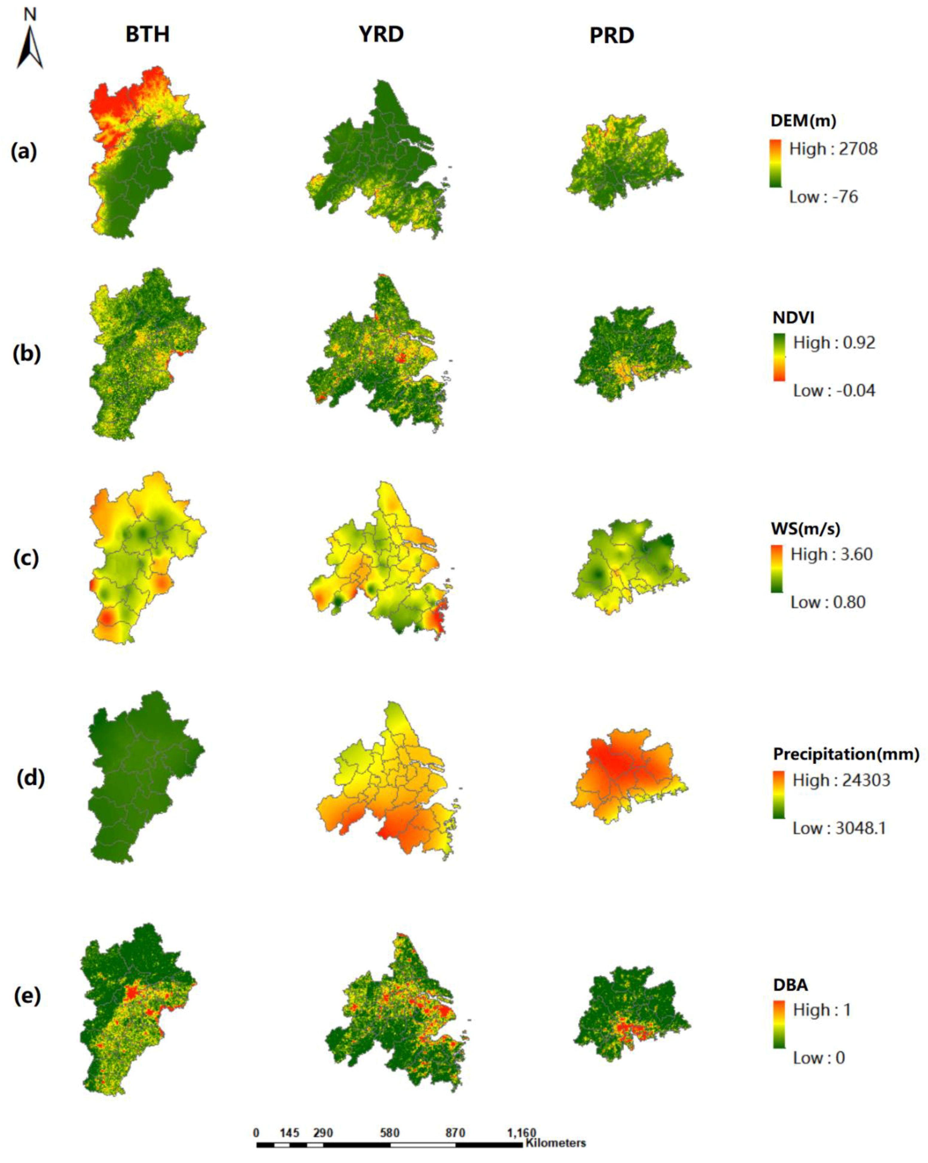
The influence of elevation on AOD has been noted in numerous studies [7,9,29]. He et al. [7] discovered that the highest AOD values are more likely to be found in flat areas with low elevation, whereas in mountainous areas or highland areas, the AOD values are generally low. In addition, Li et al. [9] also showed that the spatial distribution of AOD is significantly influenced by terrain. Therefore, terrain was selected as one of the impact factors in this study. Specifically, a global DEM (see Figure 2a), which describes the ground elevation information and has a wide application scope, was used as the data source to reflect the terrain in the study area. The global DEM, at a 1-km spatial resolution, was generated by Data Central, Institute of Geographic Sciences and Natural Resources Research, Chinese Academy of Sciences (http://www.resdc.cn/).
(ii) Normalized Difference Vegetation Index
A negative relationship between the NDVI and AOD was widely reported [30]. Since vegetation has the ability to absorb atmospheric particulates, high NDVI areas are more likely to be covered by a low AOD [9]. Therefore, the NDVI at a 1-km resolution was selected as one of the potential impact factors (see Figure 2b). The NDVI data were obtained from Data Central, Institute of Geographic Sciences and Natural Resources Research, Chinese Academy of Sciences (http://www.resdc.cn/).
(iii) Precipitation and wind speed (WS)
The relationship between meteorological factors and aerosols was reported by Jin et al. [31] and Lau and Kim [32], who proved that precipitation and wind speed have a significant impact on the distribution of aerosols. In this case, we selected wind speed and precipitation as potential impact factors (see Figure 2c,d). The precipitation data was obtained from Data Central, Institute of Geographic Sciences and Natural Resources Research, Chinese Academy of Sciences, with a 1-km resolution, while the wind speed, based on land-based stations, was provided by the American National Centers for Environmental Information (NCEI).
2. Land-use Cover Factor
Shengtian et al. [33] reported that the density of built-up areas and aerosols are strongly related. Therefore, we selected the density of built-up area (DBA) (see Figure 2e) from land cover data as a potential impact factor, which required two steps: converting the facet elements of the buildings into point elements, and then calculating the point density. All of these operations were handled in ArcGIS 10.2. The land-use cover data with a 1-km by 1-km resolution was obtained from Data Central, Institute of Geographic Sciences and Natural Resources Research, Chinese Academy of Sciences (available online: http://www.resdc.cn/).
Table 1 summarizes the basic information about these potential impact factors. To make the statements more concise, we used abbreviations to express the corresponding potential impact factors.
3. Methods
3.1. Spatial Autocorrelation Analysis
Spatial autocorrelation is one aspect of spatial heterogeneity and can be measured by various indices, including Moran’s I [34], Geary’s C [35], and others [36]. The most widely used of these measures is Moran’s I [37,38,39], which provides a simple means to assess the degree of spatial autocorrelations. The value of Moran’s I ranges from −1 to 1. A value close to 1 indicates a positive autocorrelation, a value close to −1 indicates a negative autocorrelation, and a value close to 0 suggests a random spatial distribution. Moran’s I can be calculated as given in Equation (1):
where denotes the spatial weighting factor. When the spatial unit i is the neighbor of the spatial unit j, the value of is 1. Otherwise, the value of is zero [37]. The variables and are the values of X in the corresponding spatial units i and j, respectively; is the average of the X value; n is the total number of spatial units; and i represents the i-th unit.
3.2. Geographically Weighted Regression (GWR)
The GWR is an extension of the traditional standard regression [40], which are the local statistics, with a set of local parameters varying from place to place to represent the spatial heterogeneity of geographical phenomena [41]. In contrast, the normally used regression methods, such as OLS, are the global statistics, and they assume that the relationship is spatially constant. The GWR can be expressed as shown in Equation (2):
where denotes the coordinate of location i in space, represents the intercept value, is the k-th independent variable at location i, and represents the parameter for the k-th independent variable at location i.
This model allows the parameters to be locally estimated. Tu and Xia [41] noted that the GWR takes the spatial locations of samples into consideration, which shows its superiority in reflecting spatially complicated relationships. The estimation of parameters is undertaken as shown in Equation (3):
where is matrix whose diagonal elements denote the geographical weighting of the observation data for observation i, and the off-diagonal elements are zero. The weights matrix is computed for each point i at which the parameters are estimated.
The core of the GWR model is the spatial weighting function, which is critical for the correct estimation of the model parameters. The most commonly used spatial weighting functions are the Gaussian function and bi-square function. Referring to an existing study [42], the Gaussian function was used in our study, and by Gaussian function, the weights can be calculated using Equation (4):
where b is a nonnegative parameter known as the bandwidth, which produces a decay of influence with distance between locations i and j. In contrast, the bi-square function (Equation (5)) can adjust the bandwidth automatically, based on the density of the sample:
where is the Euclidean distance between location i and location j, and b is the bandwidth.
In this study, 987, 946, and 941 random points in the BTH, YRD, and PRD were sampled as the input of GWR. The points were generated randomly by the Create Random Points tool in ArcGIS; then, we used the Extract Values to Points tool in ArcGIS to extract the values of the independent and dependent variables at the location of the points.
4. Results and Discussion
4.1. Spatial Distribution of AOD and Its Potential Impact Factors for the Metropolises
A high AOD was found in the urban areas in these three regions. Figure 1 displays the annual mean AOD for these three metropolises. Spatially, the high AOD values were clustered in the urban areas. Specifically, the southern and central parts of the BTH experienced high AOD values, such as in Beijing, Tianjin, Shijiazhuang, Tangshan, Xingtai, Baoding, and Handan, which are the most developed areas of China, with large areas of built-up land. This situation also occurred in the north of the YRD, especially in Yancheng, Suzhou, Shanghai, and Nantong. However, although most parts of Guangdong Province have high build-up densities, lower AOD values were observed. This is partly because typhoons and heavy rains frequently occur in these zones [20].
Moran’s I indices were calculated to represent the spatial distribution of the AOD, and they suggest different degrees of spatial autocorrelations for the study areas. Specifically, 987, 946, and 941 random points in the BTH, YRD, and PRD, respectively, were sampled. The Moran’s I values, along with Z-scores and p-values, are listed in Table 2, and they suggest obvious and varying spatial autocorrelations in the spatial distribution of the AOD in our study areas. The Z-scores are simply standard deviations and the p-value is a probability. The Z-score and p-value indicate the confidence levels of the results. In our study, based on the listed Z-scores and p-values, 99% confidence levels have been achieved. Therefore, according to these confidence results, among these metropolises, the spatial distribution of AOD in the BTH suffered the highest spatial autocorrelation, with a Moran’s I score of 0.940. The AOD in the YRB and PRD suffered a mitigated but also evident spatial autocorrelation, with a Moran’s I of 0.715 and 0.680, respectively. The Moran’s I suggests that there is a less than 1% likelihood that this clustered pattern of AOD could be the result of random chance in these three metropolises.
To determine the potential driving factors for the AOD in the metropolises, a Pearson correlation analysis was carried out to clarify the general relationships between the AOD and the potential driving factors. As the results show in Table 3, the significances of the correlations between all potential factors and the AOD are less than 0.05, which is statistically significant.
The results of the Pearson correlation analysis are consistent with existing studies, but the degree varies. In our case, the AOD values are always positively correlated with the DBA values, which is consistent with previous studies [43,44]. More specifically, the DBA had the strongest positive influence on the AOD value in the BTH (0.60) and PRD (0.58), but their relation becomes weaker in the YRD (0.46). A negative relationship between the NDVI and AOD is found in the BTH, YRD, and PRD, with −0.19, −0.62, and −0.63, respectively. Negative coefficients have also been declared in He et al.’s (2016) [7] study for all of China and Li and Wang‘s study for Guangdong Province. There is an obviously negative relationship between the DEM and AOD in these metropolises: −0.86 in the BTH, −0.69 in the YRD, and −0.60 in the PRD. On the other hand, the correlation analysis suggests the relationships between the WS and precipitation did not have a significant relationship with the AOD in our case, which conflicts with previous conclusions [31,32]. It is possible that because the area of each study region is too small, these meteorological factors are relatively stable in each region, and in this case, the WS and precipitation were not selected as the driving factors. To be specific, we chose the factors with correlation coefficients larger than 0.5 as the independent variables to carry out the GWR.
4.2. Factor Analysis by GWR and OLS-Based Regression
4.2.1. Model Validation
The GWR is better at addressing problems with autocorrelated spatial distributions, and OLS-based regression can address normal problems. To make a comparison, the GWR- and OLS-based regressions were carried out simultaneously for the three metropolises. The diagnoses of the GWR and the OLS models are provided in Table 4.
The GWR model performs much better in the impact factors analysis of the AOD with higher R-squared values, lower corrected Akaike Information Criterion (AICc) and lower spatial clustering of residuals than that of the OLS. Taking the BTH as an example, the R-squared value of the GWR is 0.94 for DBA, while that of OLS is much lower (only 0.36). In addition, the AICc is a criterion for evaluating the results of regression models, which estimates the relative quality of statistical models [45]. The AICc has the advantage of tending to be more accurate than the AICc (especially for small samples). The AICc value of the OLS is larger than that of the GWR, suggesting that the GWR model performs better than the OLS model in this study area [40]. As seen in Table 4, there are large gaps between the AICc values of OLS and GWR, especially in the BTH, the AICc values of OLS are −388.55 and −1269.04 larger than that of the GWR for the DBA and DEM, respectively. Moreover, the GWR evidently reduced the spatial clustering of the residuals by using the Moran’s I index. The Moran’s I values of the residuals in the OLS model are higher than those of the GWR model (see Table 4) in our study areas for all independent variables. Specifically, for example, the Moran’s I value of the residuals in the OLS for the PRD, with the DEM as the independent variable, is 0.59, and the Moran’s I value dropped to 0.03 in the same regions with the same independent variable by the GWR. A similar improvement was also found in the GWR with the DBA and NDVI as the independent variables, respectively.
The diagnoses suggest a better performance of the GWR model in our case study. The GWR significantly improved the R-squared values and reduced the spatial clustering of the residuals in the region with autocorrelation. The diagnosis guarantees the accuracy of the results of the GWR, which are shown and discussed in the following section.
4.2.2. Spatially Varying Relationship between AOD and Its Impact Factors
The GWR discovered spatially varying coefficients for the independent variables (see Figure 3, Figure 4 and Figure 5 for BTH, YRD, and PRD, respectively). In general, the coefficients are consistent with the results of existing studies and coefficients achieved by the OLS (see Table 5), but they vary from place to place.
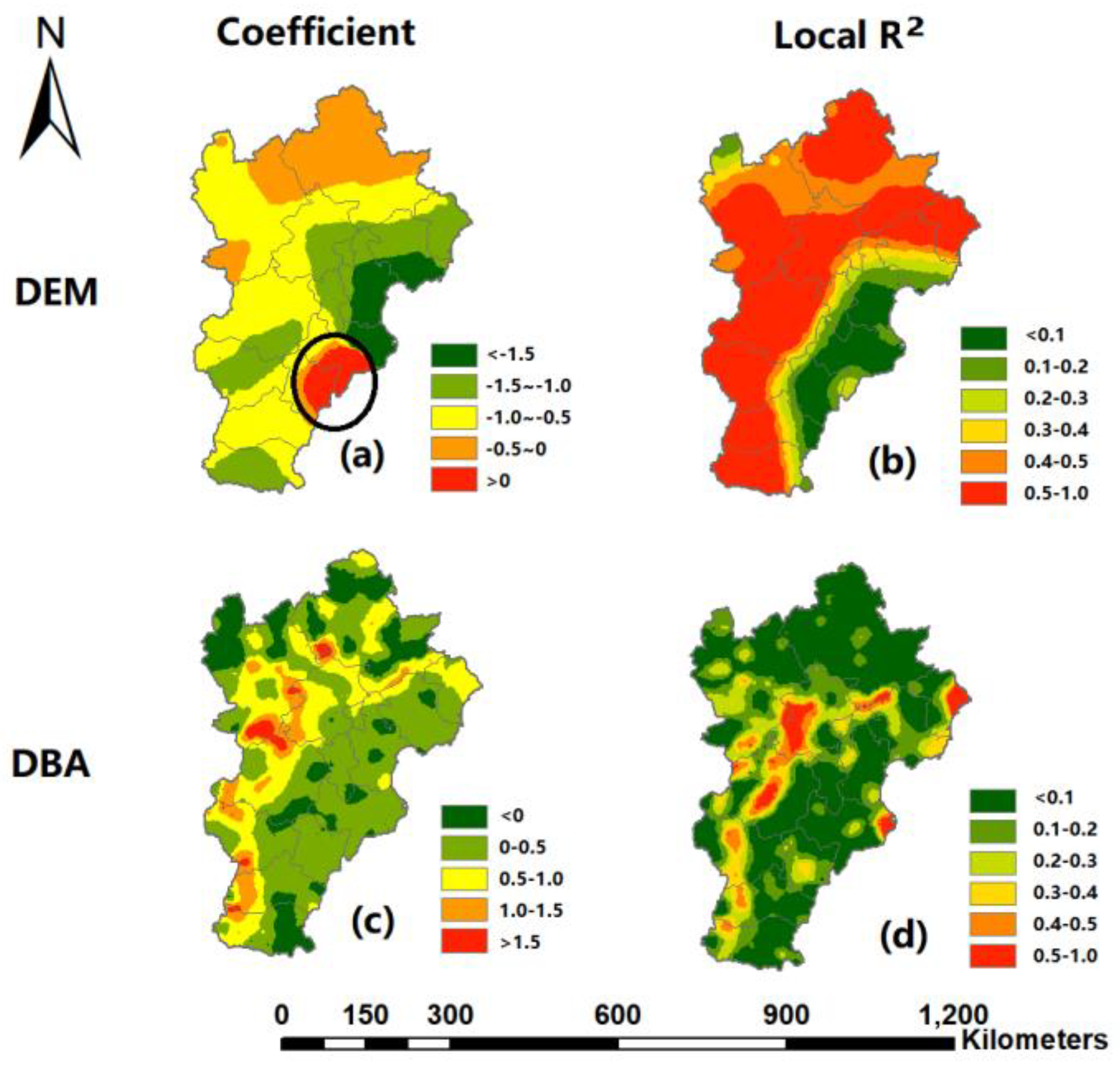
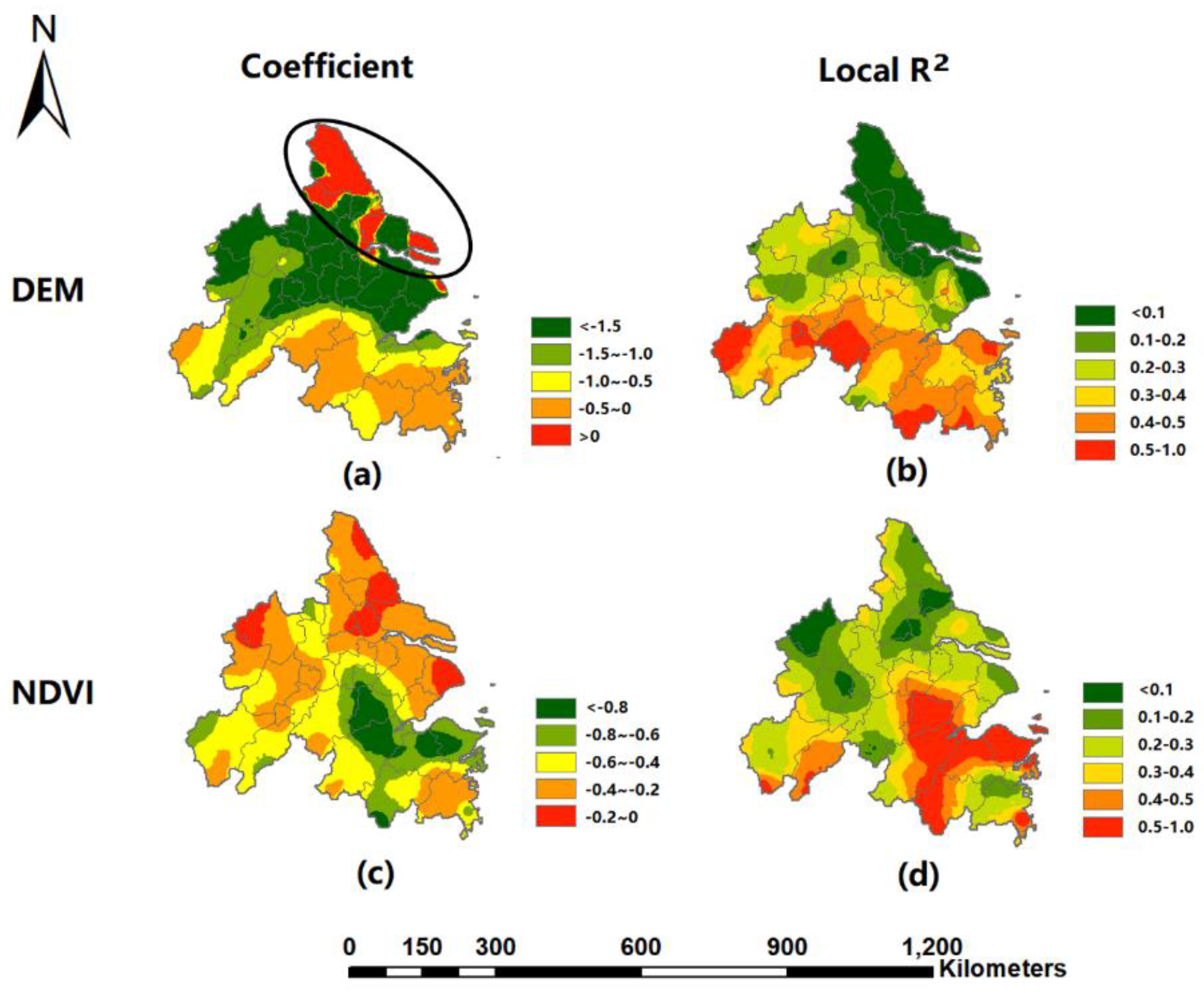
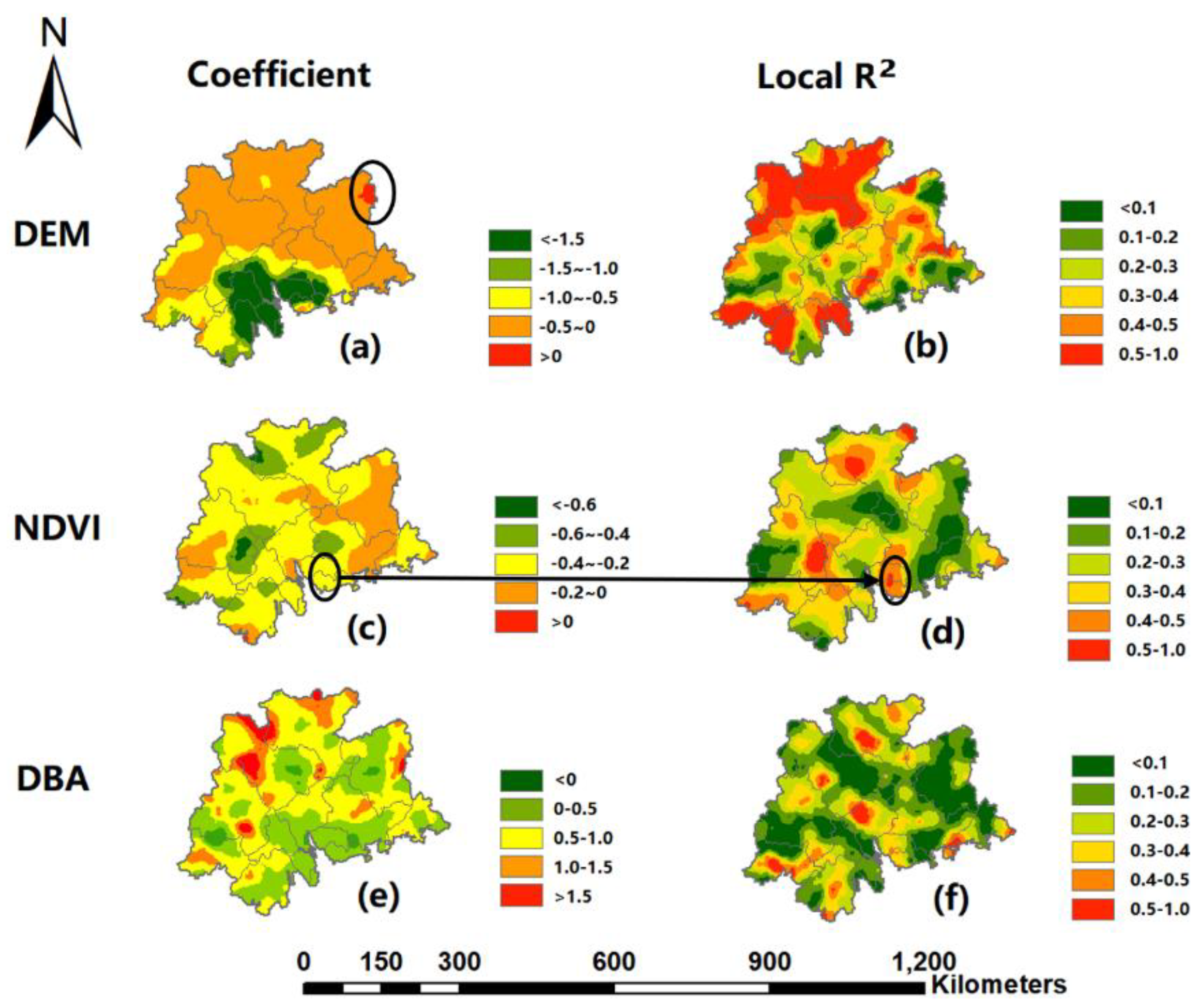
By the GWR, it was found that the elevation led to a negative impact on the AOD in our case, which is consistent with the results of the OLS and existing studies, but it indicates that the DEM cannot explain the aerosol increases in the plain areas, such as the urban areas of the BTH and YRD. A positive coefficient has been found in some places, while the corresponding R-squared values in these areas are relatively low (see the marked places in Figure 3a, Figure 4a and Figure 5a). It indicates that in these places, the DEM is not a significant factor contributing to the AOD variation. For example, in the southeastern regions of the BTH (Tianjin, Cangzhou City), the R-squared value is less than 0.1 (see Figure 3b), and it suggests that in developed areas, the variation of the DEM would not explain the change of the AOD. Similarly, the R-squared values of the DEM in the most developed urban area of the YRD (Shanghai, Yangzhou, Yancheng, Nantong) are also very low, ranging from 0.1 to 0.2. It is possible that population and energy emissions will contribute to the majority of aerosol increases [46,47] in developed urban areas, and no obvious elevation variation exists in urban area. However, this situation changes in the PRD, where urban areas still maintain a stronger negative coefficient of DEM, and the R-squared (greater than 0.4) is higher than that of the other two metropolises. Taking Shenzhen in PRD as an example, there are mountains in cities, and an obvious AOD drop has been found in mountains. As a result, a strong negative with a higher R-squared impact of DEM on AOD was found in these areas.
The DBA has a positive impact on the AOD increase by the GWR, and according to the spatially varying R-squared value, that strong positive impact is only reliable in the area with a higher DBA. In most parts of BTH, the coefficient of DBA is steady at 0 to 1, with an R-squared value approximately 0.1, which suggests that the DBA cannot explain the change of the AOD. However, in the places with a higher DBA, the R-squared value increased to approximately 0.4, and the value of the coefficient grew to above 1. Similarly, in the PRD, the DBA led to evident impact on an aerosol increase merely in the place with a larger area of built-up land and a higher DBA, where a larger R-squared value existed. In the area with no built-up land, the R-squared value dropped to under 0.1. This R-squared value differs from the results provided by the OLS with a constant coefficient of 1.19 and 0.69 in the BTH and PRD, respectively. The results of OLS suggested a constant strong positive impact of the DBA on aerosols in all metropolises, whereas the GWR showed that strong positive impacts merely existed in the places with a higher DBA.
The GWR showed a negative impact of the NDVI on aerosol increases in the YRD and PRD, and that impact is stronger in areas with greater vegetation coverage than in the places covered by built-up land. In the YRD, the places with R-squared values greater than 0.4 are those in places with a higher NDVI and are far away from the built-up land. In these places, a strong negative impact of the NDVI has been found, with a coefficient less than −0.6. A similar condition can be found for PRD. However, we also find a negative impact of the NDVI in the urban places with R-squared values larger than 0.4 (see the marked places in Figure 5c,d). This negative impact is weaker with a coefficient of approximately −0.2~−0.4. It suggests that in the PRD, the NDVI has a strong negative impact on aerosols in the places with high NDVI values that are far away from urban areas, and it also relieves the aerosols in the urban areas, but this impact is weaker.
5. Conclusions
In this study, we analyzed the spatial variation of MODIS-retrieved aerosols over the BHT, YRD, and PRD in 2015, according to the Moran’s I values of the AOD, and we suggest that there were obvious spatial autocorrelations in our case, which is an aspect of spatial heterogeneity. After that, the correlation analysis between the AOD and its potential impact factors was carried out to select impact factors for each region with which the GWR was carried out. The GWR is better than the OLS in identifying the impact factors of aerosols, and it improves the R-squared value, reduces the AICc values, and reduces the autocorrelation of the residuals.
The spatial heterogeneity in the AOD distributions and their impact factors for three metropolises has been proven in various aspects. First, the Moran’s I index of the AOD varied from 0.94 to 0.68 in these three metropolises. It suggests that the AOD in the BTH suffered a strong spatial autocorrelation and spatial clustering, while the degree spatial autocorrelation dropped in the PRD, with a more spreading spatial distribution of the AOD. Second, the Pearson correlation analysis on the AOD and its impact factors discovered that the impact factors of the AOD in metropolises are different.
According to the results of the GWR, the impact varied from place to place. Specifically, even though a negative impact of the DEM on the AOD was found and the conclusion is consistent with existing studies [7,30], in the BTH, the DEM can only explain the aerosol decrease in the places with large terrains and cannot explain the aerosol decrease in the places with low terrains, which are usually the urban areas. Similar conditions also existed in the YRD. However, for the PRD, due to the large number of mountains in the cities and the elevation changes in many of the urban areas, there is still a strong negative relationship between elevation and aerosol in urban areas. Being different from existing studies, which found that the DEM made a negative impact on aerosols for an entire region, the GWR suggests that only in the places with higher terrains would the DEM lead to a negative impact. For the impact of the NDIV, the GWR determined a negative relationship between the NDVI and the AOD, and an existing study also found a negative relationship [7]. However, this negative impact is strong in the places with larger vegetation coverage and weak in the urban area with less vegetation coverage, according to the results of the GWR. When considering the impact of the DBA, it also found that in the places with higher urban development, there is a larger R-squared value and it suggests that only in these places is the positive impact of the DBA on aerosol reliable.
The spatial heterogeneity of air quality, including autocorrelation and non-stationarity, has been widely studied [48,49], but few studies have included spatial heterogeneity in factor analysis by using the GWR model to address this problem. This study looked at the heterogeneity of the AOD in the BTH, YRD, and PRD, and conducted the factor analysis by GWR rather than by OLS. The results are reliable and considerable. They clarify that even in the same region, one impact may specifically affect aerosols in limited places. In fact, the GWR has been widely used in spatial relationship analyses in different fields [50,51], while few studies used it in the field of factor analysis for AOD. In our case, the GWR not only significantly improved the value of R-squared and reduced the autocorrelation in the residuals but also provided reliable and reasonable results. For future studies, the GWR can be used for the impact factor analysis of AOD under multiple spatial scales, and more considerable impact factors, such as population, GDP, and road density, can be added.
Acknowledgments
Financial support was provided by the National Natural Science Foundation of China under grant No. 41601415. The authors would also like to thank Data Central, Institute of Geographic Sciences and Natural Resources Research, the Chinese Academy of Sciences, for providing the land-use data sets.
Author Contributions
Hui Shi performed the main experiments and wrote part of the paper; Qingqing He provided the basic data; Wenting Zhang provided guidance throughout the research and analyzed the data.
Conflicts of Interest
The authors declare no conflict of interest.
References
- Guoshun, Z.; Ronghul, H.; Mingxing, W. Great progress in study on aerosol and its impact on the global environment. Prog. Nat. Sci. 2002, 12, 407–413. [Google Scholar]
- Mao, L.; Qiu, Y.; Kusano, C.; Xu, X. Predicting regional space–time variation of PM 2.5 with land-use regression model and MODIS data. Environ. Sci. Pollut. Res. 2012, 19, 128–138. [Google Scholar] [CrossRef] [PubMed]
- Yan, X.; Shi, W.; Luo, N.; Zhao, W. A new method of satellite-based haze aerosol monitoring over the North China Plain and a comparison with MODIS Collection 6 aerosol products. Atmos. Res. 2016, 171, 31–40. [Google Scholar] [CrossRef]
- Kampa, M.; Castanas, E. Human health effects of air pollution. Environ. Pollut. 2008, 151, 362–367. [Google Scholar] [CrossRef] [PubMed]
- Liu, X.; Chen, Q.; Che, H.; Zhang, R.; Gui, K.; Zhang, H.; Zhao, T. Spatial distribution and temporal variation of aerosol optical depth in the Sichuan basin, China, the recent ten years. Atmos. Environ. 2016, 147, 434–445. [Google Scholar] [CrossRef]
- Kaufman, Y.J.; Tanré, D.; Remer, L.A.; Vermote, E.F.; Chu, A.; Holben, B.N. Operational remote sensing of tropospheric aerosol over land from EOS moderate resolution imaging spectroradiometer. J. Geophys. Res. Atmos. 1997, 102, 17051–17067. [Google Scholar] [CrossRef]
- He, Q.; Zhang, M.; Huang, B. Spatio-temporal variation and impact factors analysis of satellite-based aerosol optical depth over China from 2002 to 2015. Atmos. Environ. 2016, 129, 79–90. [Google Scholar] [CrossRef]
- Guo, Y.; Hong, S.; Feng, N.; Zhuang, Y.; Zhang, L. Spatial distributions and temporal variations of atmospheric aerosols and the affecting factors: A case study for a region in central China. Int. J. Remote Sens. 2012, 33, 3672–3692. [Google Scholar] [CrossRef]
- Li, L.; Wang, Y. What drives the aerosol distribution in Guangdong-the most developed province in Southern China? Sci. Rep. 2014, 4, 5972. [Google Scholar] [CrossRef] [PubMed]
- Feng, X. Research on Spatial Correlation Between Air Quality and Land Use Based on GWR Models. Nat. Environ. Pollut. Technol. 2017, 16, 155. [Google Scholar]
- Dormann, F.C.; McPherson, M.J.; Araújo, B.M.; Bivand, R.; Bolliger, J.; Carl, G.; Kühn, I. Methods to account for spatial autocorrelation in the analysis of species distributional data: A review. Ecography 2007, 30, 609–628. [Google Scholar] [CrossRef]
- Zhang, L.; Bi, H.; Cheng, P.; Davis, C.J. Modeling spatial variation in tree diameter–height relationships. For. Ecol. Manag. 2004, 189, 317–329. [Google Scholar] [CrossRef]
- Mcmillen, D.P. Geographically weighted regression: The analysis of spatially varying relationships. Am. J. Agric. Econ. 2002, 86, 554–556. [Google Scholar] [CrossRef]
- Brunsdon, C.; Fotheringham, A.S.; Charlton, M.E. Geographically weighted regression: A method for exploring spatial nonstationarity. Geogr. Anal. 1996, 28, 281–298. [Google Scholar] [CrossRef]
- Fotheringham, A.S.; Charlton, M.E.; Brunsdon, C. Geographically weighted regression: A natural evolution of the expansion method for spatial data analysis. Environ. Plan. A 1998, 30, 1905–1927. [Google Scholar] [CrossRef]
- Haas, J.; Ban, Y. Urban growth and environmental impacts in Jing-Jin-Ji, the Yangtze, River Delta and the Pearl River Delta. Int. J. Appl. Earth Obs. Geoinform. 2014, 30, 42–55. [Google Scholar] [CrossRef]
- Cui, Y.Z.; Lin, J.T.; Song, C.; Liu, M.Y.; Yan, Y.Y.; Xu, Y.; Huang, B. Rapid growth in nitrogen dioxide pollution over Western China, 2005–2013. Atmos. Chem. Phys. 2016, 15, 34913–34948. [Google Scholar] [CrossRef]
- Xing, Z. Seasonal variation of mass absorption efficiency of elemental carbon in the four major emission areas in China. Aerosol Air Qual. Res. 2014, 14, 1897–1905. [Google Scholar] [CrossRef]
- Zhou, L.; Jiang, Z.; Zhaoxin, L.I.; Yang, X. Numerical simulation of urbanization climate effects in regions of east China. Chin. J. Atmos. Sci. 2015, 39, 596–610. [Google Scholar]
- Li, L.; Qian, J.; Ou, C.Q.; Zhou, Y.X.; Guo, C.; Guo, Y. Spatial and temporal analysis of Air Pollution Index and its timescale-dependent relationship with meteorological factors in Guangzhou, China, 2001–2011. Environ. Pollut. 2014, 190, 75–81. [Google Scholar] [CrossRef] [PubMed]
- Nichol, J.; Bilal, M. Validation of MODIS 3 km Resolution Aerosol Optical Depth Retrievals Over Asia. Remote Sens. 2016, 8, 328. [Google Scholar] [CrossRef]
- Xiao, Q.; Zhang, H.; Choi, M.; Li, S.; Kondragunta, S.; Kim, J.; Holben, B.; Levy, R.C.; Liu, Y. Evaluation of VIIRS, GOCI, and MODIS Collection 6 AOD retrievals against ground sunphotometer measurements over East Asia. Atmos. Chem. Phys. 2016, 16, 20709–20741. [Google Scholar] [CrossRef]
- He, Q.; Zhang, M.; Huang, B.; Tong, X. MODIS 3 km and 10 km aerosol optical depth for China: Evaluation and comparison. J. Atmos. Environ. 2017, 153, 150–162. [Google Scholar] [CrossRef]
- Ma, Q.; Li, Y.; Liu, J.; Chen, J.M. Long Temporal Analysis of 3-km MODIS Aerosol Product Over East China. IEEE J. Sel. Top. Appl. Earth Obs. Remote Sens. 2017, 10, 2478–2490. [Google Scholar] [CrossRef]
- Remer, L.A.; Kaufman, Y.J.; Tanré, D.; Mattoo, S.; Chu, D.A.; Martins, J.V.; Li, R.R.; Ichoku, C.; Levy, R.C.; Kleidman, R.G.; et al. The MODIS aerosol algorithm, products, and validation. J. Atmos. Sci. 2005, 62, 947–973. [Google Scholar] [CrossRef]
- Ghotbi, S.; Sotoudeheian, S.; Arhami, M. Estimating urban ground-level pm 10, using MODIS 3km AOD product and meteorological parameters from WRF model. Atmos. Environ. 2016, 141, 333–346. [Google Scholar] [CrossRef]
- Bilal, M.; Qiu, Z.; Campbell, J.R.; Spak, S.N.; Shen, X.; Nazeer, M. A New MODIS C6 Dark Target and Deep Blue Merged Aerosol Product on a 3 km Spatial Grid. Remote Sens. 2018, 10, 463. [Google Scholar] [CrossRef]
- Bilal, M.; Nichol, J.E.; Chan, P.W. Validation and accuracy assessment of a Simplified Aerosol Retrieval Algorithm (SARA) over Beijing under low and high aerosol loadings and dust storms. J. Remote Sens. Environ. 2014, 153, 50–60. [Google Scholar] [CrossRef]
- Bilal, M.; Nichol, J.E.; Bleiweiss, M.P.; Dubois, D. A Simplified high resolution MODIS Aerosol Retrieval Algorithm (SARA) for use over mixed surfaces. Remote Sens. Environ. 2013, 136, 135–145. [Google Scholar] [CrossRef]
- Dong, Z.P.; Yu, X.; Li, X.M.; Dai, J. Analysis of variation trends and causes of aerosol optical depth in Shaanxi province using MODIS data. Chin. Sci. Bull. 2013, 58, 4486–4496. [Google Scholar] [CrossRef]
- Jin, M.; Shepherd, J.M.; King, M.D. Urban aerosols and their variations with clouds and precipitation: A case study for New York and Houston. J. Geophys. Res. Atmos. 2005, 110, 211. [Google Scholar] [CrossRef]
- Lau, K.M.; Kim, K.M. Observational relationships between aerosol and Asian monsoon precipitation, and circulation. Geophys. Res. Lett. 2006, 33, 320–337. [Google Scholar] [CrossRef]
- Shengtian, Y.; Zhifeng, Y.; Xianqiang, M.; et al. Research on buildings impacting on aerosol diffusing in urban area using remote sensing. J. Environ. Sci. 2004, 16, 509–512. [Google Scholar]
- Moran, P.A.P. Notes on continuous stochastic phenomena. Biometrika 1950, 37, 17–23. [Google Scholar] [CrossRef] [PubMed]
- Geary, R.C. The contiguity ratio and statistical mapping. Inc. Stat. 1954, 5, 115–146. [Google Scholar] [CrossRef]
- Getis, A.; Ord, J.K. The analysis of spatial association by use of distance statistics. Geogr. Anal. 1992, 24, 189–206. [Google Scholar] [CrossRef]
- Thompson, E.S.; Saveyn, P.; Declercq, M.; Meert, J.; Guida, V.; Eads, C.D.; Robles, E.S.; Britton, M.M. Characterisation of heterogeneity and spatial autocorrelation in phase separating mixtures using Moran’s I. J. Colloid Interface Sci. 2018, 513, 180–187. [Google Scholar] [CrossRef] [PubMed]
- Tiefelsdorf, M. Modelling Spatial Processes: The Identification and Analysis of Spatial Relationships in Regression Residuals by Means of Moran’s I; Lecture Notes in Earth Sciences; Springer: Berlin/Heidelberg, Germany, 2000; Volume 87, p. 167. [Google Scholar]
- Tiefelsdorf, M.; Boots, B. The Exact Distribution of Moran’s I[M]//Modelling Spatial Processes; Springer: Berlin/Heidelberg, Germany, 2000; pp. 985–999. [Google Scholar]
- Fotheringham, A.S. Spatial variations in school performance: A local analysis using geographically weighted regression. Geogr. Environ. Model. 2001, 5, 43–66. [Google Scholar] [CrossRef]
- Tu, J.; Xia, Z.G. Examining spatially varying relationships between land use and water quality using geographically weighted regression i: Model design and evaluation. Sci. Total Environ. 2008, 407, 358–378. [Google Scholar] [CrossRef] [PubMed]
- Foody, G.M. Geographical weighting as a further refinement to regression modelling: An example focused on the NDVI–rainfall relationship. Remote Sens. Environ. 2003, 88, 283–293. [Google Scholar] [CrossRef]
- Wang, X.; Fei, Z.; Jing, Y.; Zhang, H.; Zhe, L. Relationship between land cover-landscape spatial characteristics and aerosol optical depth in Ebinur Lake Watershed. Trans. Chin. Soc. Agric. Eng. 2016, 32, 273–283. [Google Scholar]
- Hou, C.; Jiang, H.; Wang, X.; Pei, H. The spatial-temporal evolution of aerosol optical depth and the analysis of influence factors in Bohai Rim. Inst. Phys. Publ. 2014, 17, 012035. [Google Scholar] [CrossRef]
- Burnham, K.P.; Anderson, D.R. Model Selection and Multimodel Inference: A Practical Information-Theoretic Approach; Springer Science & Business Media: Berlin, Germany, 2003. [Google Scholar]
- Tie, X.; Cao, J. Aerosol pollution in China: Present and future impact on environment. Particuology 2009, 7, 426–431. [Google Scholar] [CrossRef]
- Streets, D.G.; Bond, T.C.; Carmichael, G.R.; Fernandes, S.D.; Fu, Q.; He, D.; Klimont, Z.; Nelson, S.M.; Tsai, N.Y.; Wang, M.Q.; et al. An inventory of gaseous and primary aerosol emissions in Asia in the year 2000. J. Geophys. Res. Atmos. 2003, 108, GET30-1. [Google Scholar] [CrossRef]
- Zhang, T.; Wei, G.; Wei, W.; Ji, Y.; Zhu, Z.; Huang, Y. Ground level PM2.5 estimates over china using satellite-based geographically weighted regression (GWR) models are improved by including NO2 and enhanced vegetation index (EVI). Int. J. Environ. Res. Public Health 2016, 13, 1215. [Google Scholar] [CrossRef] [PubMed]
- Van, D.A.; Martin, R.V.; Spurr, R.J.; Burnett, R.T. High-Resolution Satellite-Derived PM2.5 from Optimal Estimation and Geographically Weighted Regression over North America. Environ. Sci. Technol. 2015, 49, 10482–10491. [Google Scholar]
- Lin, C.H.; Wen, T.H. Using Geographically Weighted Regression (GWR) to Explore Spatial Varying Relationships of Immature Mosquitoes and Human Densities with the Incidence of Dengue. Int. J. Environ. Res. Public Health 2011, 8, 2798–2815. [Google Scholar] [CrossRef] [PubMed]
- Ping, L.V.; Zhen, H. Affecting factors research of Beijing residential land price based on GWR model. Econ. Geogr. 2010, 3, 472–478. [Google Scholar]
Figure 1.
The locations of study areas in China and the corresponding spatial distributions of aerosol optical depth (AOD).
Figure 1.
The locations of study areas in China and the corresponding spatial distributions of aerosol optical depth (AOD).
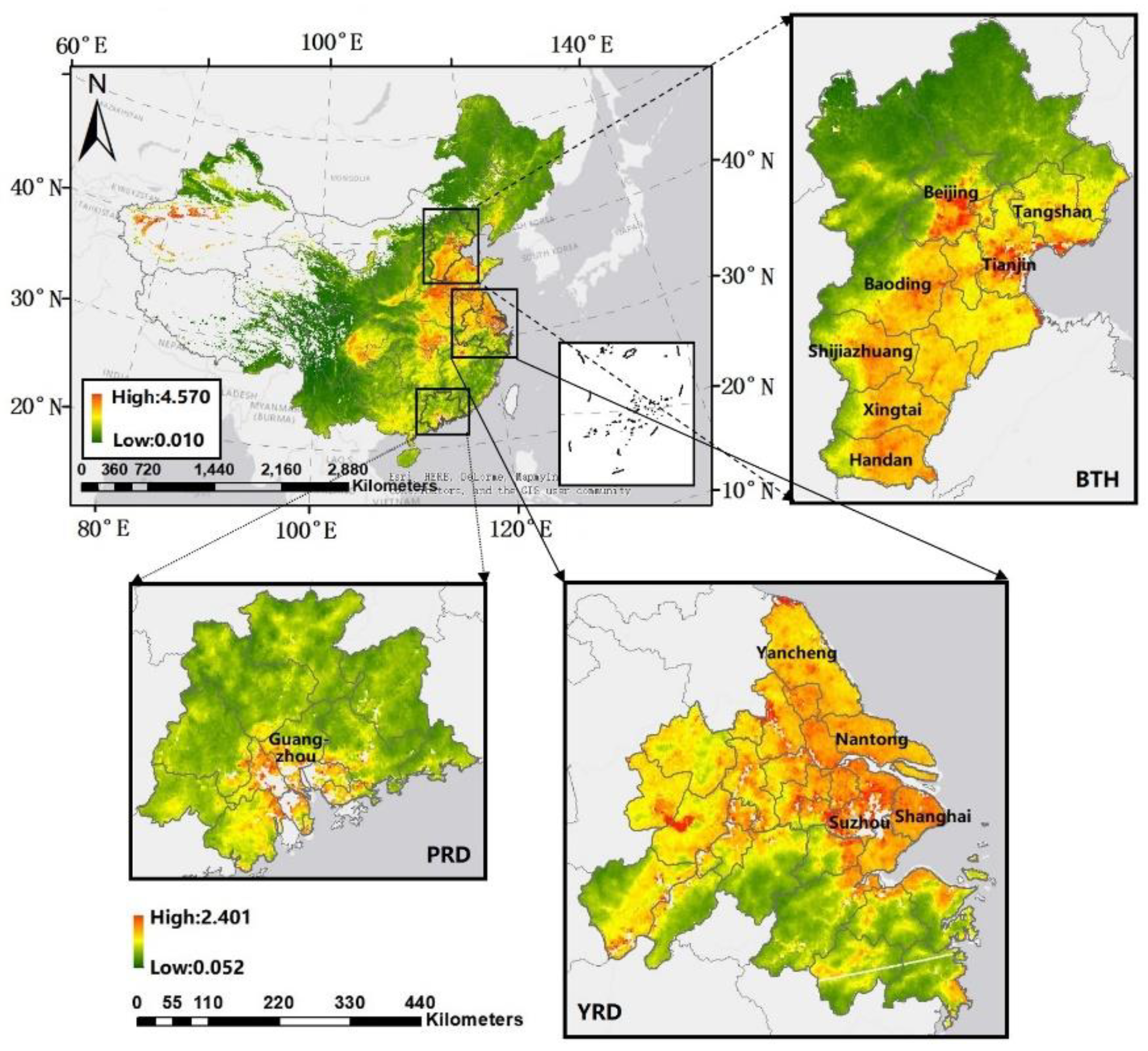
Figure 2.
Spatial distribution of potential factors in 2015.

Figure 3.
Spatial distribution of coefficients and local R2 of DEM (a,b) and DBA (c,d) by GWR in the BTH.
Figure 3.
Spatial distribution of coefficients and local R2 of DEM (a,b) and DBA (c,d) by GWR in the BTH.

Figure 4.
Spatial distribution of coefficients and local R2 of DEM (a,b) and NDVI (c,d) by GWR in the YRD.
Figure 4.
Spatial distribution of coefficients and local R2 of DEM (a,b) and NDVI (c,d) by GWR in the YRD.

Figure 5.
Spatial distribution of coefficients and local R2 of DEM (a,b), NDVI (c,d), and DBA (e,f) by GWR in the PRD.
Figure 5.
Spatial distribution of coefficients and local R2 of DEM (a,b), NDVI (c,d), and DBA (e,f) by GWR in the PRD.


Table 1.
Summary of potential impact factors.
| Type | Independent Variable | Abbreviation | Data Source | Description | Year |
|---|---|---|---|---|---|
| Natural factors | Digital Elevation Model | DEM | Data Central, Institute of Geographic Sciences and Natural Resources Research, Chinese Academy of Sciences | 1-km resolution | - |
| Normalized Difference Vegetation Index | NDVI | Data Central, Institute of Geographic Sciences and Natural Resources Research, Chinese Academy of Sciences | 1-km resolution | 2015 | |
| Wind Speed | WS | National Centers for Environmental Information (NCEI) of National Oceanic and Atmospheric Administration (NOAA) | - | 2015 | |
| Precipitation | - | Data Central, Institute of Geographic Sciences and Natural Resources Research, Chinese Academy of Sciences | 1-km resolution | 2015 | |
| Land-use cover related factors | Density of Built-up Area | DBA | Data Central, Institute of Geographic Sciences and Natural Resources Research, Chinese Academy of Sciences | 1-km resolution | 2015 |
Table 2.
Spatial autocorrelations of AOD in study areas. BTH = Beijing-Tianjin-Hebei region; YRD = Yangtze River Delta; PRD = Pearl River Delta.
Table 2.
Spatial autocorrelations of AOD in study areas. BTH = Beijing-Tianjin-Hebei region; YRD = Yangtze River Delta; PRD = Pearl River Delta.
| Study Area | Moran’s I | Z-Value | P-Value |
|---|---|---|---|
| BTH | 0.940 | 26.770 | 0.000 |
| YRD | 0.715 | 44.615 | 0.000 |
| PRD | 0.680 | 29.805 | 0.000 |
Table 3.
Correlation analysis between AOD and its potential impact factors.
| Study Area | DEM | NDVI | WS | Precipitation | DBA |
|---|---|---|---|---|---|
| BTH | −0.86 | −0.19 | −0.25 | 0.26 | 0.60 |
| YRD | −0.69 | −0.62 | 0.18 | −0.40 | 0.46 |
| PRD | −0.60 | −0.63 | 0.47 | −0.27 | 0.58 |
Table 4.
Comparison between the geographically weighted regression (GWR) and ordinary least square (OLS) models. AICc = Akaike Information Criterion.
Table 4.
Comparison between the geographically weighted regression (GWR) and ordinary least square (OLS) models. AICc = Akaike Information Criterion.
| Study Area | Impact Factor | R2 | AICc | Moran’s I of Residuals | |||
|---|---|---|---|---|---|---|---|
| OLS | GWR | OLS | GWR | OLS | GWR | ||
| BTH | DEM | 0.74 | 0.87 | −1269.04 | −1910.11 | 0.50 | 0.48 |
| DBA | 0.36 | 0.94 | −388.55 | −2283.29 | 0.69 | 0.13 | |
| YRD | DEM | 0.47 | 0.83 | −756.74 | −1607.89 | 0.50 | 0.11 |
| NDVI | 0.38 | 0.81 | −608.21 | −1579.58 | 0.56 | 0.12 | |
| PRD | DEM | 0.36 | 0.87 | −1355.72 | −2435.66 | 0.59 | 0.03 |
| NDVI | 0.39 | 0.8 | −1410.09 | −2219.33 | 0.54 | 0.19 | |
| DBA | 0.33 | 0.83 | −1317.59 | −2209.06 | 0.66 | 0.12 | |
Table 5.
The coefficients of the independent variables by OLS.
| Study Area | DEM | NDVI | DBA |
|---|---|---|---|
| BTH | −0.84 | - | 1.19 |
| YRD | −0.89 | −0.69 | - |
| PRD | −0.50 | −0.48 | 0.69 |
© 2018 by the authors. Licensee MDPI, Basel, Switzerland. This article is an open access article distributed under the terms and conditions of the Creative Commons Attribution (CC BY) license (http://creativecommons.org/licenses/by/4.0/).
Share and Cite
MDPI and ACS Style
Shi, H.; He, Q.; Zhang, W. Spatial Factor Analysis for Aerosol Optical Depth in Metropolises in China with Regard to Spatial Heterogeneity. Atmosphere 2018, 9, 156. https://doi.org/10.3390/atmos9040156
AMA Style
Shi H, He Q, Zhang W. Spatial Factor Analysis for Aerosol Optical Depth in Metropolises in China with Regard to Spatial Heterogeneity. Atmosphere. 2018; 9(4):156. https://doi.org/10.3390/atmos9040156
Chicago/Turabian StyleShi, Hui, Qingqing He, and Wenting Zhang. 2018. "Spatial Factor Analysis for Aerosol Optical Depth in Metropolises in China with Regard to Spatial Heterogeneity" Atmosphere 9, no. 4: 156. https://doi.org/10.3390/atmos9040156
Note that from the first issue of 2016, this journal uses article numbers instead of page numbers. See further details here.