Quantitative Evaluation of the Haines Index’s Ability to Predict Fire Growth Events

Pacific Northwest Research Station, USDA Forest Service, Seattle, WA 98020, USA
Atmosphere 2018, 9(5), 177; https://doi.org/10.3390/atmos9050177
Submission received: 17 April 2018
/
Revised: 3 May 2018
/
Accepted: 3 May 2018
/
Published: 8 May 2018
(This article belongs to the Special Issue Fire and the Atmosphere)
Abstract
:The Haines Index is intended to provide information on how midtropospheric conditions could lead to large or erratic wildfires. Only a few studies have evaluated its performance and those are primarily single fire studies. This study looks at 47 fires that burned in the United States from 2004 to 2017, with sizes from 9000 ha up to 218,000 ha based on daily fire management reports. Using the 0-h analysis of the North American Model (NAM) 12 km grid, it examines the performance of the start-day Haines Index, as Haines (1988) originally discussed. It then examines performance of daily Haines Index values as an indicator of daily fire growth, using contingency tables and four statistical measures: true positive ratio, miss ratio, Peirce skill score, and bias. In addition to the original Haines Index, the index’s individual stability and moisture components are examined. The use of a positive trend in the index is often cited by operational forecasters, so the study also looks at how positive trend, or positive trend leading to an index of 6, perform. The Continuous Haines Index, a related measure, is also examined. Results show a positive relationship between start day index and peak fire daily growth or number of large growth events, but not final size or duration. The daily evaluation showed that, for a range of specified growth thresholds defining a growth event, the Continuous Haines Index scores were more favorable than the original Haines Index scores, and the latter were more favorable than the use of index trends. The maximum Peirce skill score obtained for these data was 0.22, when a Continuous Haines Index of 8.7 or more was used to indicate a growth event, 1000 ha/day or more would occur.
1. Introduction
Originally published by Haines [1]—hereafter H88—as the Lower Atmospheric Severity Index, the Haines Index is intended to indicate the potential for large or erratic fires. It filled a need expressed among fire weather forecasters and fire managers for information about atmospheric conditions above ground—conditions believed capable of influencing a fire but not directly observable at the surface or incorporated in surface-based fire danger measures. The design of the Index built on the work of Brotak [2] and Brotak and Reifsnyder [3]. These works examined the co-occurrence of fire with such conditions as atmospheric instability, dry air advection, and wind shear.
The Index has two components and three elevation-based variants. The A component is a measure of static stability, in the form of the temperature difference between two specified standard pressure levels. The B component measures dryness as dewpoint depression at a specified pressure level. The pressure levels for both components depend roughly on surface elevation. The A and B components each have a value of 1 (more stable, or wetter), 2, or 3 (more unstable, or drier), and are added together to yield an Index value of 2 to 6, with 6 expected to represent high potential for large or erratic fire.
Potter [4] discusses the incomplete nature of the original work, which was acknowledged by Haines. The fire data were a small, subjectively chosen sample. The climatology was rudimentary, and despite the author’s efforts, a wind component was not included. The author also noted that the relative weighting of the A and B components, equal in the publication, should be examined. To date, only Heilman and Bian [5] and Mills and McCaw [6] document any attempt to refine or modify the Index.
A small number of publications have examined the performance of the index. Saltenberger and Barker [7] applied it to an analysis of the Oregon Awbrey Hall Fire. Werth and Ochoa [8] looked at daily index values for the Lowman and Willis Gulch fires, both in Idaho. Goodrick et al. [9] examined performance of the index on a state-wide scale for Florida, for 1998 and 1999. Fernandes et al. [10] recently examined the Haines Index and a number of other measures with respect to fires between 2500 and 25,000 ha in Portugal. These studies, collectively, do not clearly substantiate any correlative relation between the index and fire measures, such as growth, intensity, size, or duration. There are no published, peer-reviewed studies that quantitatively examine the performance of the index for multiple days of multiple, individual fires. This is an important, basic step necessary to evaluate the index—yet it has not been done in the thirty years since the Index was introduced. The available fire and weather data are a large part of the reason this has not been done, as will be discussed further in this paper.
This study examines the Haines Index, including the individual A and B components; daily trends in the index; and the Continuous Haines Index (C-Haines) [6]. (The Haines Index × turbulent kinetic energy (TKE) [5] measure was not evaluated in this study because of questions of grid resolution and what grid level or levels of TKE would be appropriate.) It looks at daily growth for a number of large fires, primarily in the western United States. Each index measure is evaluated using contingency tables and performance measures including true positive ratio, miss ratio, bias, and Peirce skill score. Performance measures are examined for sensitivity to the chosen thresholds for the index and what constitutes a “growth event”.
2. Methods
2.1. Fire Data
Fire data suitable for evaluation of danger, weather, or behavior indices is a perennial challenge for research. The only data consistently available, and even this is not without problems, are the daily size and growth data recorded for operational purposes. More recently, satellite measurements of fire radiative power are available, but spatial and temporal coverage of these measurements are much narrower. This study, because it seeks to examine numerous fires over multiple days, uses the more historic daily size records. While areal growth is not specifically what H88 states the index predicts, it is the only readily available fire characteristic, and it is of direct interest to fire managers.
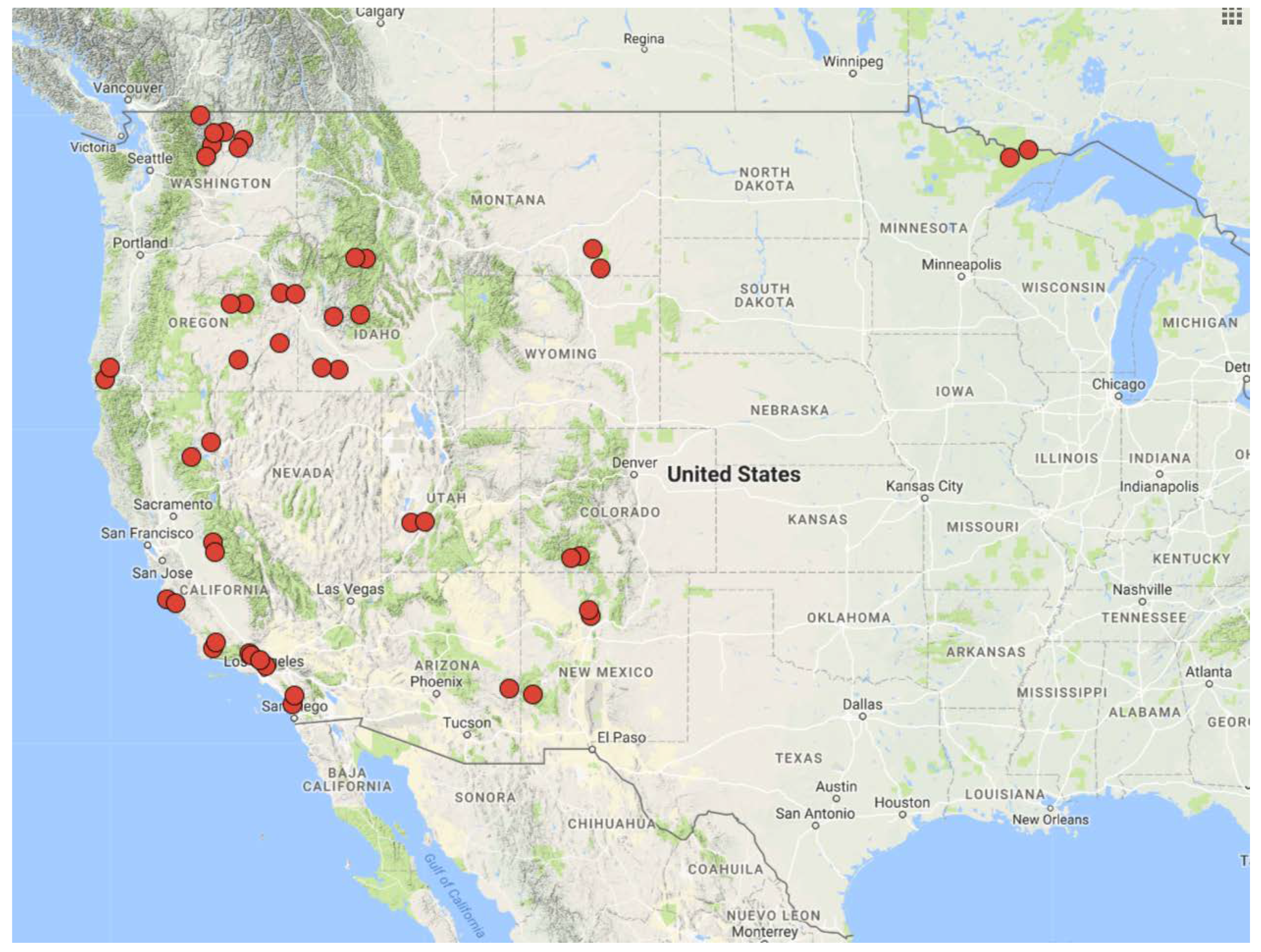
Daily growth data were acquired for 47 fires, 45 from the western United States and two from the northeastern United States (Figure 1 and Table 1). The fires were originally selected for a separate study, and comprise two sets. One set is fires over 36,400 ha, the other set is fires between 8100 and 30,400 ha, chosen primarily for their proximity to the fires in the first set. The separation of the two sets for the separate study was not maintained for this analysis. The fires in the combined set range from 9000 ha to 218,000 ha in final size, and occurred between 2004 and 2017. Growth data came from four sources: archived fire progression maps, ICS-209 reports, incident infrared (IR) overflight measurements, and the national daily Incident Management Situation Report (IMSR). In comparing the four sources for individual fires, it became clear that the individual daily IR overflight data were most accurately date-stamped. These size measurements and time stamps generally, but not always, carried over to the progression maps. Because the IR flights occur at night, their observations do not appear in the ICS-209 reports until the next afternoon, typically. And what appears in the ICS-209 reports does not get carried into the IMSR until the next day. Thus the ICS-209 sizes are often the fire’s size at the end of the previous day and the national report is yet another day behind. When this sort of lag could be confirmed, data were adjusted to match the progression or IR sizes and growth, with the ICS-209 or situation report sizes only being used to fill gaps in the progression or IR records. (Sometimes the IR data do not get filed correctly, or the progression map skips a day.) Fires for which progression or IR measurements were not available were not individually adjusted in any way. Because of these quality control measures, final fire sizes and end dates listed in Table 1 may not agree with official fire sizes or dates.
Fire growth was measured in three different ways for this study. The simplest growth measure was daily areal growth for each day i, ΔAi. The main focus of the analyses examines this growth metric, as it is the one most readily usable by the operational fire community.
The second measure was the ratio of each day’s areal growth, divided by the lifetime average daily area growth for that fire. This measure identifies anomalously large or small area increases, relative to the rest of a given fire:
where is the areal growth ratio for day i, D is the fire’s duration and Afinal is the fire’s final size. The third measure is slightly more complicated. It reflects the fact that a given increase in area represents a higher rate of spread when it occurs on a small fire, rather than a large fire. To reflect this, each day’s area is converted to the radius of a circle of the same area. The difference in successive days’ radii is then compared to the average radial growth rate over the fire’s life-time, producing what could be considered a relative measure of equivalent circle radial growth. Mathematically, this is determined as:
where the relative radial growth for day i. Whenever there was a gap in the growth data, the days of missing data and the first day with a new size reported were dropped from the analysis for all growth measures.
2.2. Meteorological Data
Mid-tropospheric temperature and dewpoint data for the Haines Index were obtained from the National Weather Service’s North American Model (NAM) 0000 UTC analysis, 0-h forecast. The NAM grid 218, with grid spacing of 12 km, was used. Data at the requisite pressure levels for the mid- or high-level HI were extracted for the grid point nearest to the ICS-209 listed location of each fire. This usually corresponds to the location of the fire start. None of the fires studied were in the low-elevation HI variant area.
Haines Index A and B components (HIA and HIB) were computed from the NAM data, retaining the actual temperature differences and dew point depressions used to obtain the integer index values. These same data determine the C-Haines.
2.3. Analysis and Statistical Methods
There are two primary analyses applied here, one of which has several subdivisions. The first analysis considers the index’s performance on the terms originally used and considered [1]. Specifically, the value of the HI on the day each fire started is considered as an indicator of that fire’s overall potential for large or explosive growth. The 47 fires are sorted based on first-day HI and examined to determine whether higher values of the index correspond to fires that are ultimately larger, last longer, or experience episodes of greater growth. For this analysis, growth is only considered in terms of hectares per day.
While H88 [1] used start-day index, the first published studies examining its performance [7,8] compared daily index values with daily fire behavior observations. This is also the way the index has been used operationally since its introduction. The second analysis examines the daily index values and daily growth. These are treated as dichotomous categorical events—the index says there will be a “growth event”, or not, and a growth event does or does not occur. Weather forecasting has a long history of evaluating categorical forecast skill for severe storms, tornadoes, or heavy precipitation events [11,12,13,14,15,16,17]. The present study is in essence an evaluation of forecast skill for the 0-h Haines Index “forecast” to predict a growth event. It uses contingency-type scores to examine whether there is a correlation between a categorical index and fire growth.
Based on the aforementioned forecast evaluation protocols, the second analysis here uses the following metrics (see Table 2): true positive ratio (TPR), miss ratio (MR), bias (B), and Peirce’ skill score (PSS, also known as the True skill score or statistic, Hanssen–Kuipers discriminant, or Kuipers’ performance index) [18]. The TPR answers the question “Of all of the times the index predicted an event, how often were there actually events?” The MR answers the question “Of all the times the index predicted no event, how many times was there actually an event?” Bias is the ratio of event predictions to event occurrences. Ideally, a predictor has a bias score of 1. The PSS is an equitable skill score, meaning that random predictions and constant predictions have equal scores, zero, and a perfect predictor will have a score of 1. Values of PSS below zero indicate that using the predictor has lower skill than randomly assigning each day to a growth or non-growth category.
In operational meteorology, the hit rate and false alarm rate are more commonly used than TPR and MR. Wilks [17] refers to hit rate and false alarm rate as elements in the likelihood-base rate factorization and TPR and MR as elements in the calibration-refinement factorization. Questions answered by the latter measures are stated above. Hit rate answers the question “Of all the times the event occurred, how many were correctly predicted?” and false alarm rate answers the question “Of all the times there was no event, how many times was an event wrongly predicted”. The calibration-refinement factorization has an advantage in operational application, in that it allows one to consider the predictor’s performance at the time the prediction is made, rather than needing to wait until the predicted event or nonevent has occurred, or not.
There is no clear or formal cutoff for either the index or for growth events. The skill metrics are computed for varying thresholds on each of these. Table 3 summarizes the threshold values considered for the indices examined, and for each of the three growth measures discussed previously.
The second analysis, examining daily index performance has three major components. The first directly examines the original index, HI, and its two components, HIA and HIB. The second examines two trend-based applications of the index. Many operational users consider an increase in the Haines Index more important than the actual value. I examine the performance of an increase in the index, regardless of the magnitude of the index, and I then examine the performance when only an increase that leads to an index value of 6 constitutes a prediction of a growth event. This analysis also examines the performance of the C-Haines [6] for daily growth.
To reflect the uncertainty in actual growth dates for the fires, performance measures are computed for the data both according to the dates determined through the comparison of the various fire records, and with the growth data for all fires shifted to one day prior.
In the analyses looking at daily growth, the pairings of index measure and growth metric can require wordy descriptions. For brevity, an ordered-pair notation is adopted of the form (index = index threshold, growth metric = growth threshold). Thus, (HI = 5, ΔA = 500 ha) refers to the case where a Haines Index of 5 or more was considered the predictor, and a size increase of 500 ha or more for the day is an actual event. The abbreviations HIA and HIB will be used for those respective components of the index, +dt will indicate an increase in the index from the previous day, +dt6 will indicate “index increases to a value of 6” as noted above, and CH indicates the C-Haines.
Results are reported first using ΔA as the growth metric, and without the growth days shifted to adjust report dates. This is followed with brief summary comments regarding the other two growth measures, and the shifted-date results.
3. Results
3.1. Start-Day Index
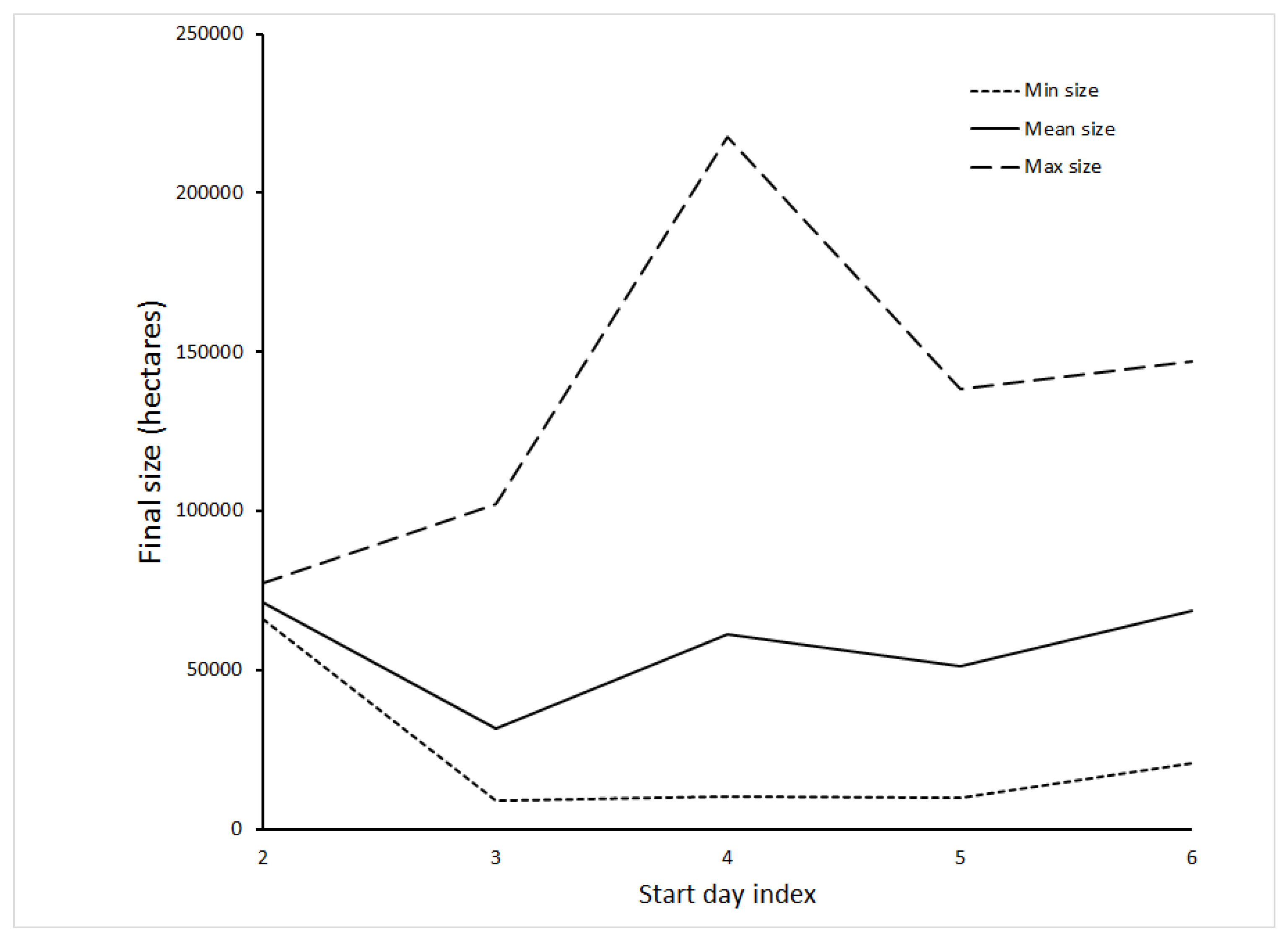
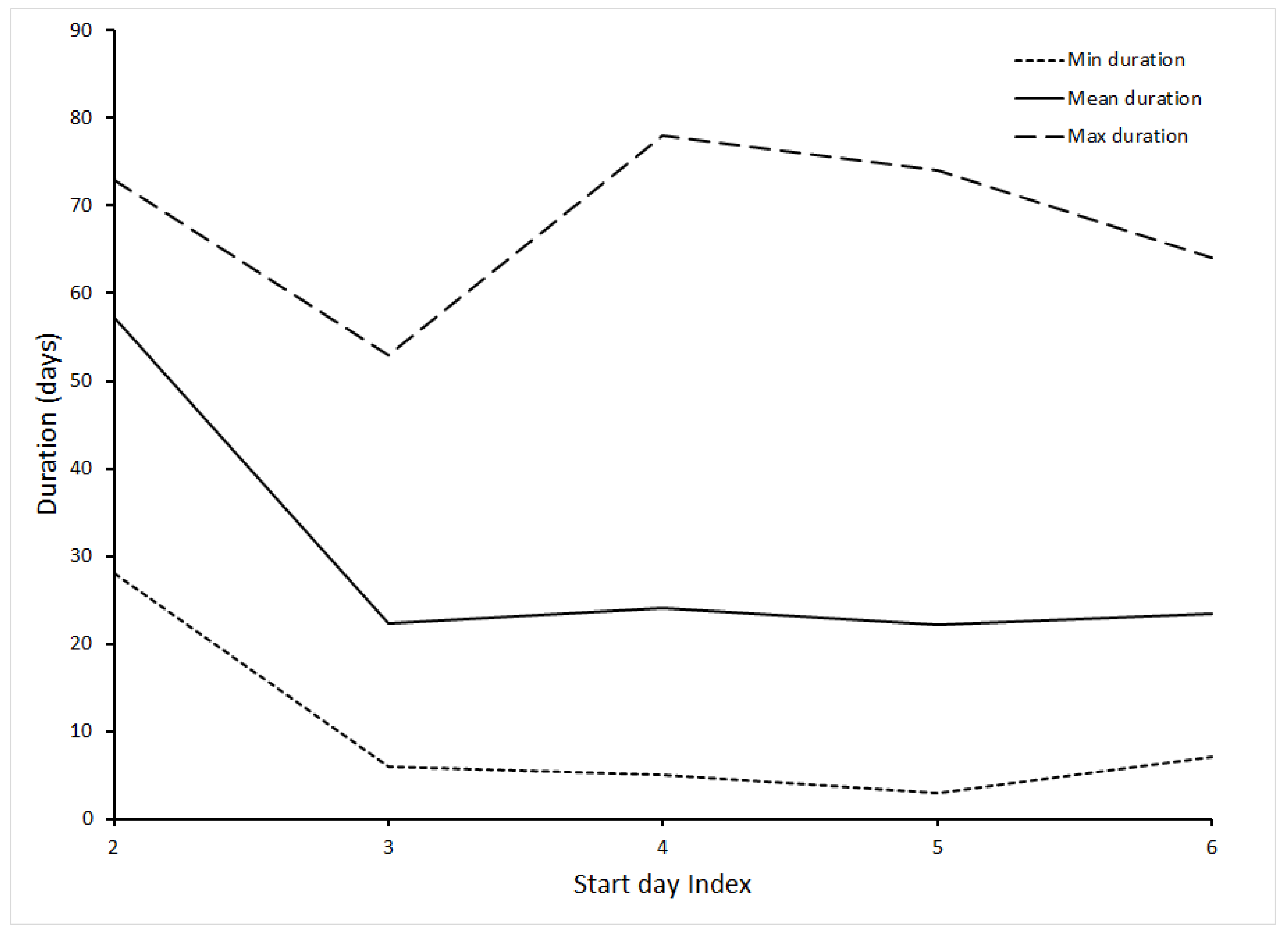
Table 4 and Figure 2, Figure 3 and Figure 4 summarize the results of start-day index results. Figure 2 shows that mean fire size was slightly greater for fires with an index of 2 on start days than any other starting day index. The smallest mean fire size was for those starting on days with index values of 3, and mean size increases thereafter. The relationship between fire duration and for the fires in this study appears in Figure 3. Mean duration was greatest for fires with a start-day index of 2; the minimum duration of any fire with a start-day index of 2 was 28 days, greater than the minimum duration of fires for any other start-day index value, and greater than the mean duration for start-day indices of 3 through 6.
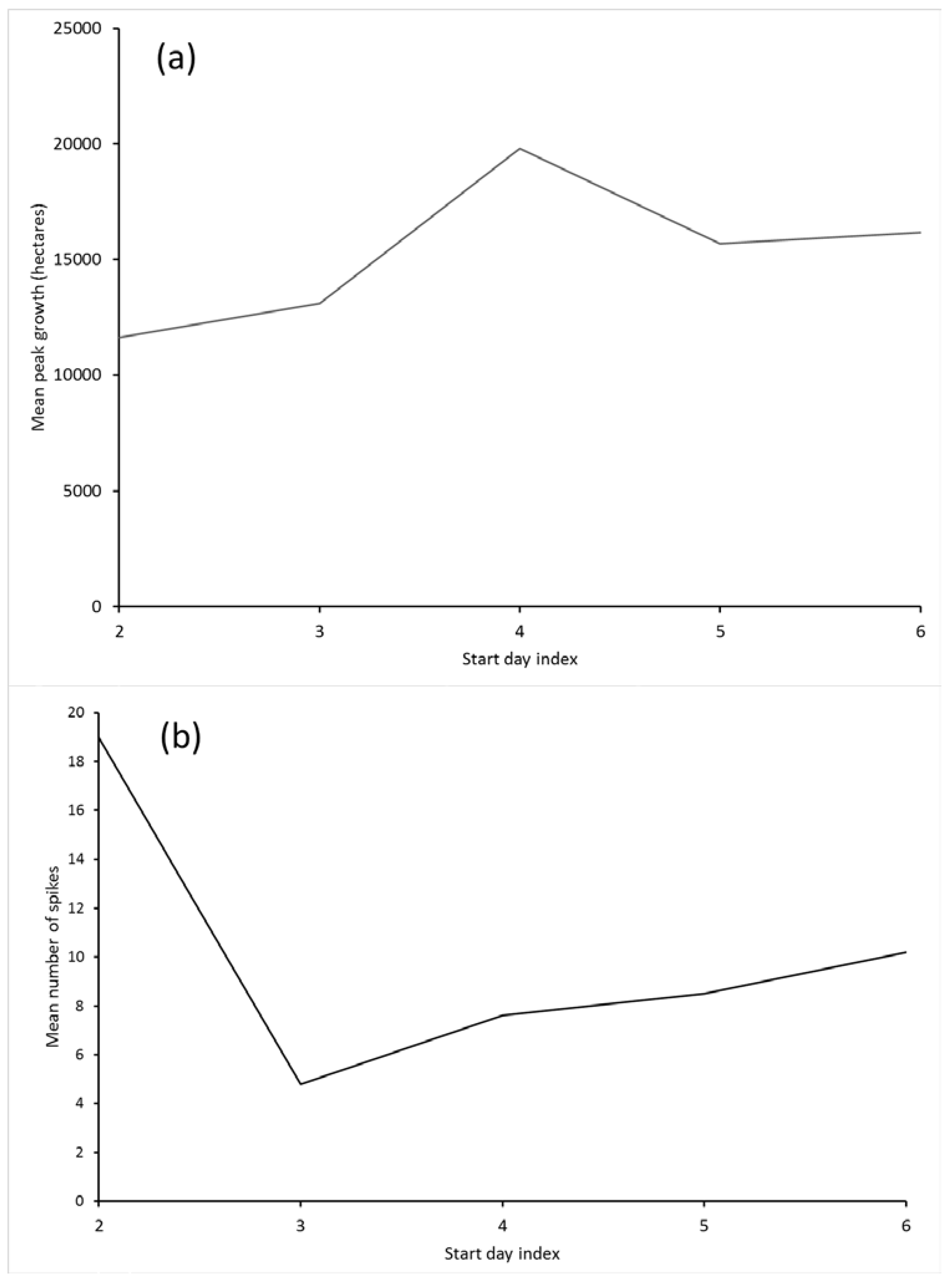
Daily growth is a more commonly considered measure of a fire’s behavior than size. It is the metric considered by Saltenberger and Barker [7] and Werth and Ochoa [8]. Figure 4 shows how start-day index related to daily growth for the study set. In Figure 4a, the mean of the peak growth day for all fires with a given starting index is shown; Figure 4b shows the mean number of spikes exceeding 1000 ha for fires with a given starting index. Mean peak growth increases with increasing start-day index, with a spike at an index of 4 primarily due to one fire. Mean number of spikes is greatest for start-day index values of 2, and all three fires with start-day index value of 2 contributed to this high value.
3.2. Original Haines Index and Components
Figure 5 shows the statistical scores for the daily Haines Index, HIA and HIB. For both HI = 6 and HI = 5 thresholds (Figure 5a), the TPR and MR values are similar to one another, and decrease with increasing growth threshold. For any given growth threshold, TPR is greater when the index threshold is HI = 6, while MR scores are almost equal for the two index thresholds tested. For the individual HIA and HIB components (Figure 5b), TPR and MR both decrease with increasing growth threshold. Each score is similar between the two index components.
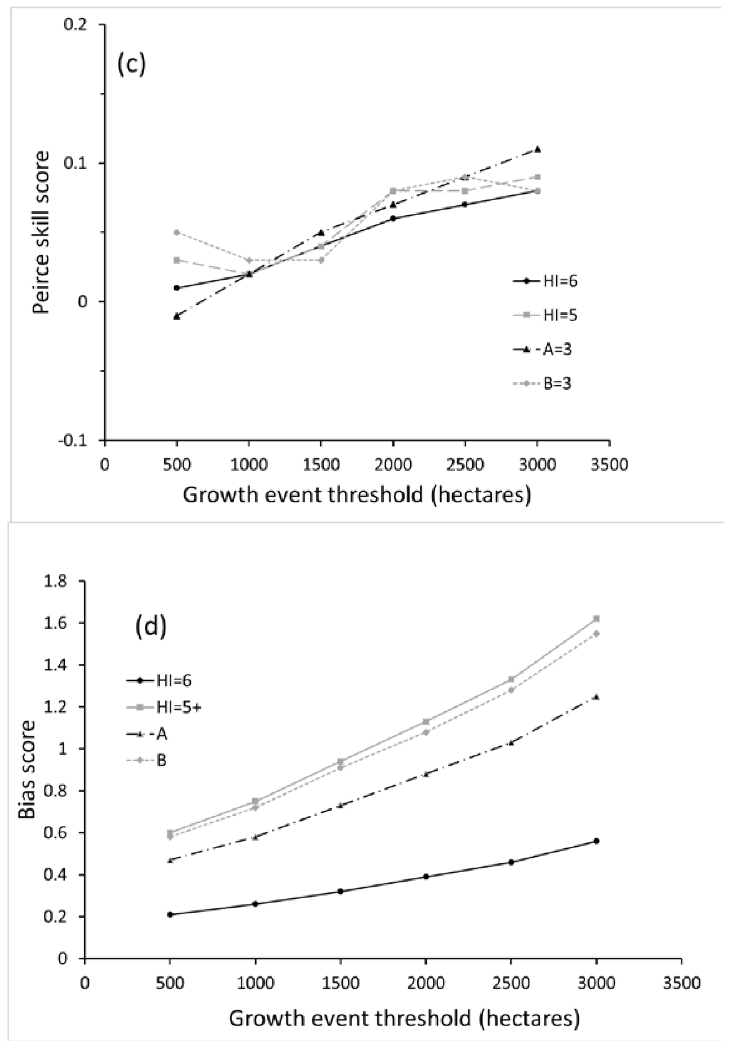
Figure 5c shows PSS for the various indices and growth thresholds. Skill is lowest for the lower growth thresholds, even negative for (HIA = 3, ΔA = 500 ha). It increases for both index thresholds and both index components, reaching a maximum of 0.11 for (HIA = 3, ΔA = 3000 ha). Skill was greater for the full index with a threshold of 5 than with a threshold of 6.
Bias scores, B, are shown in Figure 5d, increasing for all index thresholds and index components as growth threshold increases. Increasing B is a consequence of the number of index-based predictions staying constant, while the number of growth events, in the denominator of B, decreases with increasing growth threshold. Regardless of the growth threshold, B for the index threshold of 6 is lowest, with a maximum value of 0.6, indicating that the index predicts events less often than events occur. Bias scores for the thresholds HI = 5 and HIB = 3 are similar to one another at all growth thresholds, both having B = 1 for growth thresholds between 1500 and 2000 ha. The HIA curve lays intermediate to these two curves and the HI = 6 curve, and attains B = 1 near a growth threshold of 2500 ha.
3.3. Index Trend
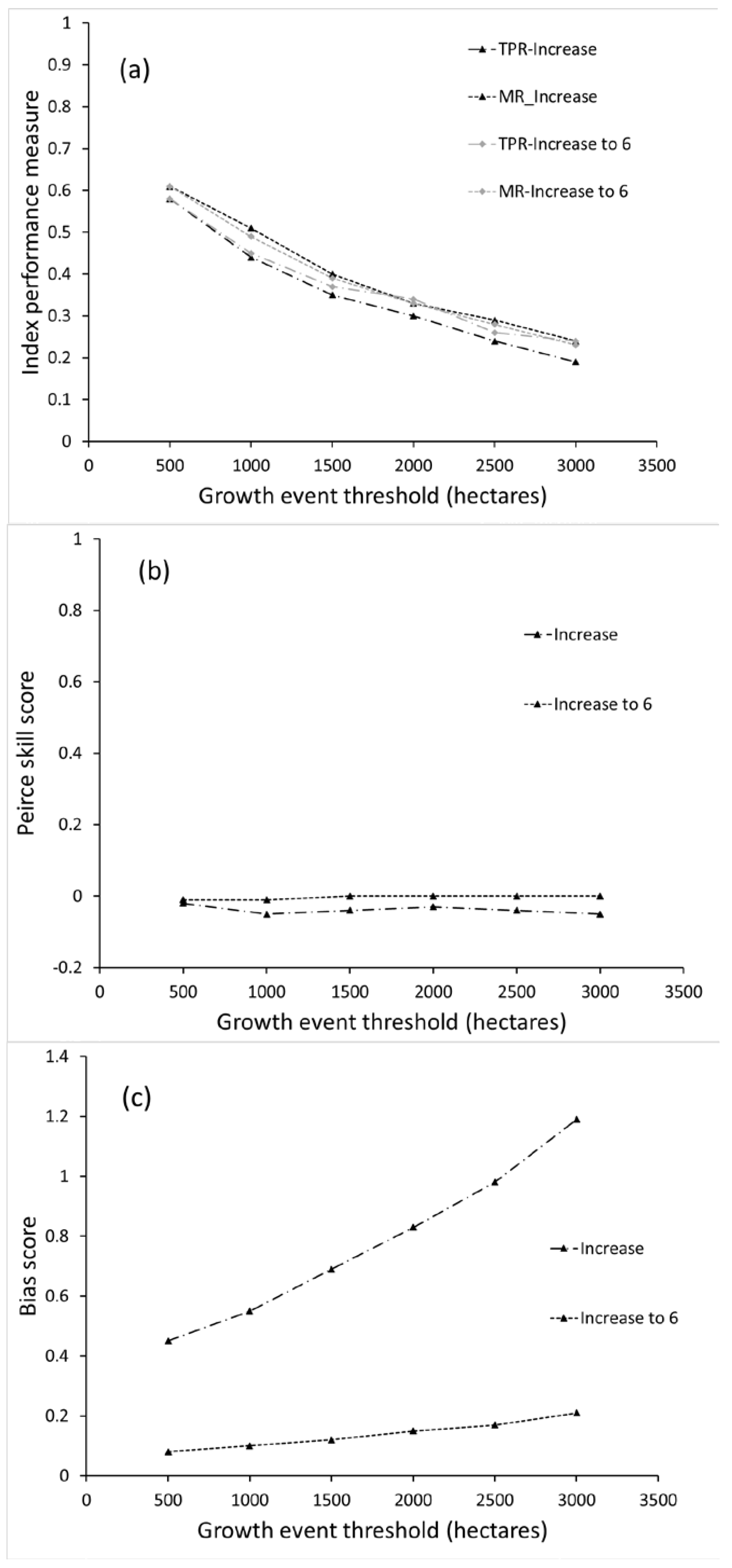
Results for the analyses using +dt and +dt6 appear in Figure 6. Figure 6a shows that the TPR and MR scores are similar to those for the basic index; for any given index measure and growth threshold, TPR and MR are similar to each other, and both decrease with increasing growth threshold. However, for both +dt and +dt6, MR exceeds TPR. For +dt, PSS is negative for all growth thresholds (Figure 6b). PSS is negative for +dt6 when growth threshold is 500 or 1000 ha, and zero for higher thresholds. Bias (Figure 6c) is less than 1 for +dt with growth thresholds below 2000 ha, but greater than 1 for higher growth thresholds. Bias for +dt6 is always less than 1, a result largely due to the relative rarity of events where the Haines Index increases to a value of 6.
3.4. C-Haines
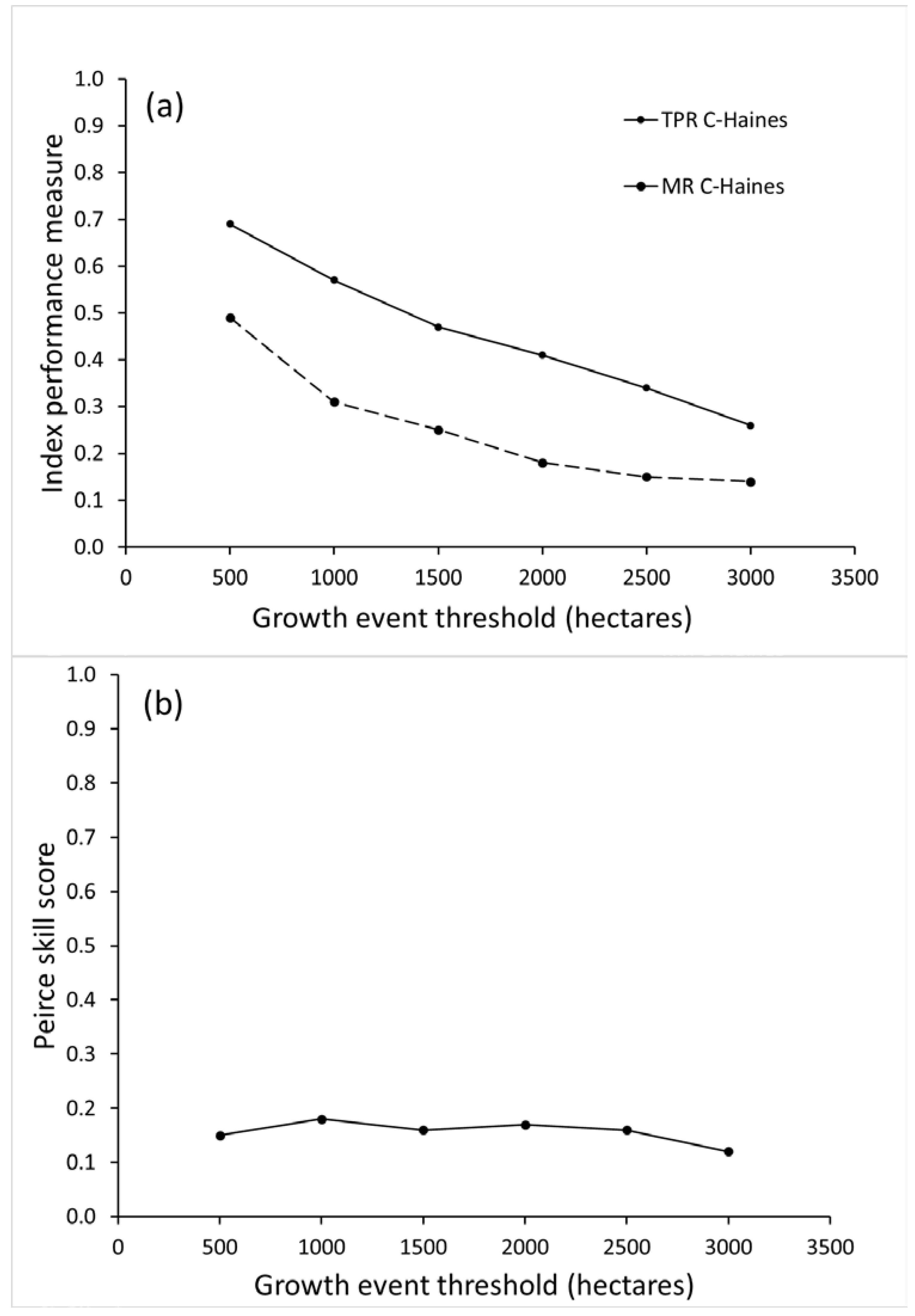
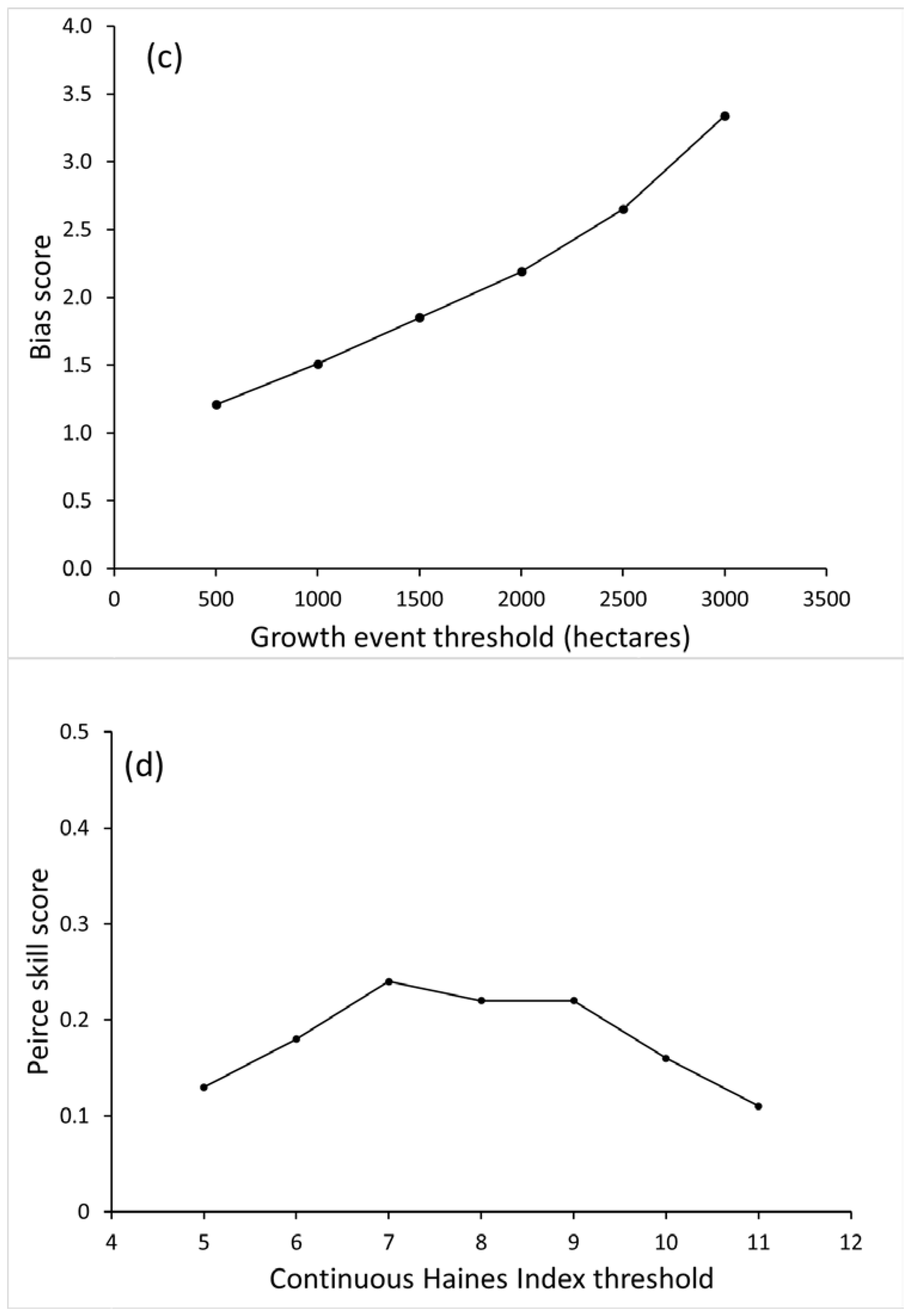
All of the scores for CH are slightly higher than the basic index scores (Figure 7), for a given growth threshold. The difference between TPR and MR (Figure 7a) is larger for CH than for the basic index, also. Trends in the scores are similar to those for the basic index—TPR and MR decrease as growth threshold increases, B increases as growth threshold increases (Figure 7b). All PSS values (Figure 7c) are greater for CH than for the basic index, and while PSS decreases with increasing growth threshold for the basic index, with a threshold of 5 or 6, it reaches a maximum value for a growth threshold of 1000 ha with the CH.
Since one of the intentional changes incorporated in the CH is that it can increase beyond 6, index thresholds of 6 to 10 were examined. Figure 7d shows PSS values for a growth threshold of 1000 ha, and indicates a peak PSS of 0.24 for a CH threshold of 7. Additional testing of both growth and index thresholds (not shown) revealed that the highest PSS and the B closest to 1 occurred for a (CH = 8.7, ΔA = 1000 ha). For these thresholds, PSS = 0.21, TPR = 0.62, and MR = 0.41.
3.5. Other Growth Measures and Lagged Fire Data
The TPR and MR values when growth events were identified by or over the ranges shown in Table 3 were roughly half those for growth in hectares. In contrast, B values were higher for the alternative growth measures (but comparable to one another) and PSS values were comparable for all three growth measures. Shifting the growth data by one day to allow for possible reporting lag made only minor difference in any of the scores, for a given index, index threshold, and growth threshold (not shown).
4. Discussion
For the 47 fires in this study, high values of the Haines Index on fire start day do not appear to correspond to overall fire size or duration. When the mean peak-day growth of fires is averaged based on start-day index, there is a slight positive slope. The growth value for a start index of 4 is heavily influenced by one fire, but otherwise there is a positive trend in the growth values—from roughly 12,000 ha for an index of 2, to 16,000 ha for an index of 6. These averages likely reflect the range of fire sizes chosen for this study, and if smaller fires were included, the difference would necessarily decrease.
The number of growth spikes appears to be extremely high for fires starting on days with HI = 2, and then shows a positive slope for index values of 3 to 6. The spike for a start-day value of 2 is due to the fact that there are only three fires in that group, and one of them had a 73-day duration, allowing time for many spikes. The number of spikes roughly doubles, from 5 for a start-day index of 3 to 10 for a start day index of 6.
Interpretation of the performance measures for daily comparisons is complex. Marzban and Lakshmanan [19] describe the importance of the relative costs of correct and incorrect forecasts when interpreting contingency table scores. When the cost of forecasting an event that does not occur differs greatly from the cost of forecasting that no event will occur but it actually does, the operational significance of the scores is not the same as it is when the two costs are comparable. Thus, the ultimate evaluation of what scores are acceptable is based on social values and beyond the scope of this number-driven paper. The discussion here focuses on relative values of the performance measures for the index thresholds and variants considered, and for the different thresholds used to define growth events.
The TPR and MR scores are similar to one another for any given growth threshold and for a specific choice of the basic Haines Index and its threshold (5 or 6, in this study). The same is true for the index components. Recall that these two performance measures answer the questions “Of all the times the index predicted an event, how often were there actually events?” (TPR) and “Of all the times the index predicted no event, how many times was there actually an event?” (MR). In this study, as long as the index threshold was held constant, as it was for each line in Figure 4a,b, the denominator in the measure was also constant, and all that changed was the numerator. The decreasing numerator as the growth event threshold increased is the cause of all change in the measures. For low growth event thresholds, TPR and MR are closer in value, indicating that basically, the index is right about events happening as often as it is wrong about non-events. For higher growth event thresholds, the difference in the performance measures increases, showing that the index correctly predicts events more often than it incorrectly predicts non-events.
As noted in Methods, the calibration-refinement factorization allows consideration of the TPR and MR scores at the time a forecast is made. For example, consider the case with (HI = 6, ΔA = 1000 ha). If, at some time and location, the Haines Index is 6, then this can be weighed in combination with the earlier result that 51% of the time when an event is predicted (HI = 6), there really is an event (growth of 1000 ha or more that day), based on TPR. Conversely, if the Haines Index is less than 6, one can use the MR to see that 47% of the time when the index does not predict an event, an event does in fact occur. Such a statement is not possible when the likelihood-base rate factorization is used.
The Peirce Skill Scores for the index with a threshold of either 5 or 6 to indicate an event, and for the separate HIA and HIB components, are less than 0.1 for all growth event thresholds, with one exception. That exception is for (HIA = 3, ΔA = 3000 ha), which has PSS = 0.11. Even that highest PSS is closer to the random-forecast score (PSS = 0) than it is to a perfect-forecast score (PSS = 1), and the growth event threshold of 3000 ha in a day is a very high threshold for the fires in this sample, let alone for fires with smaller final size.
In terms of bias, using an index threshold of 6 to identify events and requiring a bias score of 1 would require using a growth threshold of 14,000 ha in a day, but for this pair of thresholds, one must accept a PSS of 0.1, a TPR of 0.2 and a MR of 0.1. In short, an index threshold of 6 predicts too few growth events to possibly predict all actual events. Looking again at the best-case scenario for PSS, (HIA = 3, ΔA = 3000 ha), B is 1.3, indicating events were predicted 30% more often than they occurred.
The fact that the performance measures did not change appreciably when the fire data were shifted one day is not entirely surprising. The PSS values for the unshifted data are close to what one would get for random predictions, and a one-day shift could be considered a random prediction. Serial correlation in the index would make the shifted data nonrandom, but the similarity of the measures suggests the index predictions are still, essentially, random.
Using an increasing index trend to predict growth events yields lower scores for TPR, MR, and PSS than did any of the basic index applications. Not only were trend TPR scores lower than basic index TPR scores, and the same true for MR and PSS in place of TPR, but when an increasing index is used as the predictor of a growth event, MR is greater than TPR for any chosen growth event threshold—the predictor is wrong about non-events more often than it is right about events. The Peirce skill scores for trend-based predictions are on the order of 10−2, where 0 is equivalent to a random or constant value prediction. Some values of PSS are negative, indicating that the index-trend predictor for that growth event threshold is correct less often than a constant or random prediction would be.
For the C-Haines, three of the four performance scores are favorable, compared to the basic index scores. The C-Haines TPR scores, for a given growth threshold, are higher. The MR scores are lower, as well as more separated from the TPR scores for given growth thresholds. For example, for the basic index with a threshold of 5, with growth threshold of 1000 ha, TPR is 0.49, and MR is 0.47, but for C-Haines with the same threshold, TPR is 0.57 and MR is 0.31. Peirce skill scores are higher for C-Haines than for the basic Haines Index, though still closer to random or constant than they are to a perfect predictor. Bias scores for the C-Haines are higher than for the basic index at the same growth threshold, exceeding one for the lowest threshold tested and increased more rapidly as the event growth threshold increased. For the maximum PSS case noted earlier, (CH = 7, ΔA = 1000 ha), B is 1.4, indicating more predictions than actual events. However, it is possible to decrease B with only a small decrease in PSS by using (CH = 8.7, ΔA = 1000 ha).
The data set used in this study included only fires over 9000 ha, and this will have affected the results. Smaller fires would necessarily have smaller growth events, and it is likely that a threshold below 500 ha would yield different performance scores for one or all of the variations tested here. Because the larger fires used in this study are less common in the eastern United States, the performance of the Haines Index and the C-Haines on eastern fires cannot be determined with any confidence based on the present data set and analysis.
To obtain a large sample size for fires, in terms of both number of fires and fire days, it was necessary to use fire size and growth data as the predictand. This remains as problematic and limiting as it has ever been, with size errors, missing days, and in most cases inaccurate time stamps for the sizes. Haines (1988) did not specify what fire measure was used for the original index development, but given what was available at the time, size or duration is really the only possibility. It is possible that with currently available satellite and other remotely sensed data, other fire measures could be used to look for relationships between the Haines Index or the C-Haines and fire.
The meteorological data from the NAM are among the highest resolution data available for an extended historical period. Because the NAM is also one of the primary National Weather Service operational models, it is also one used frequently by incident meteorologists and forecast offices. There are newer, higher resolution models, as well as coarser resolution models that have been run further into the past. Results of a similar analysis using one of these would differ from the current results, as would analysis using raw observational soundings. Using a 0-hour analysis, rather than a model initialization, for this study, provided the best estimate of the relevant meteorological properties, and so reduced the likelihood that model characteristics are the cause of any particular finding.
5. Conclusions
Based on a multi-fire, multi-day data set, and the 0-h NAM analysis, this study characterized the ability of the Haines Index to indicate large fire growth. Both start-day index, as used by Haines [1], and daily index values as commonly used operationally, were considered using standard forecast verification measures. The results show that the measures depend on the definition of a growth event as well as what level of the index is used to predict an event. The results clearly showed, however, that using an increasing trend in the index, instead of the index itself, to determine high growth days leads to worse overall performance. The Continuous Haines Index [6], with a threshold of 8.7, correctly predicted growth events over 1000 ha more often than the original Haines Index did, mis-predicted nonevents less often, had a relatively high Peirce skill score, and had no bias. Combining the Haines Index with near-surface TKE [5] was not examined in this study. Such an evaluation requires a number of decisions regarding what NAM pressure level(s) of TKE to use, and model resolution might affect the results. The scale of such an effort merits a study in its own right, and is a potential topic for future work.
Management decisions for wildland fires incorporate a vast array of factors, such as infrastructure at risk, resources available, fuel conditions, weather conditions, firefighter safety, public safety from fire and smoke, and cost effectiveness. The relative weights of these factors are highly dependent on the specific situation, and the uncertainty or reliability of any data used in the decisions is an important piece of information. While it is not possible to say with authority that a certain TPR, MR, PSS, or B for the Haines Index is acceptable or not for all situations, these scores each provide fire weather forecasters and fire managers with more information than just the value of the index.
Acknowledgments
The author thanks the reviewers and editor for their helpful and prompt input. He would also like to thank Don Haines for his continued observations and encouragement in pursuing this work. This study was not funded by any grants and was solely produced by funding through the National Fire Plan at the USDA Forest Service’s Pacific Wildland Fire Sciences Laboratory.
Conflicts of Interest
The author declares no conflict of interest.
References
- Haines, D.A. A lower atmospheric severity index for wildland fire. Natl. Weather Dig. 1988, 13, 23–27. [Google Scholar]
- Brotak, E.A. A Synoptic Study of the Meteorological Conditions Associated with Major Wildland Fires. Ph.D. Thesis, Yale University, New Haven, Connecticut, 1977. [Google Scholar]
- Brotak, E.A.; Reifsnyder, W.E. An investigation of the synoptic situations associated with major wildland fires. J. Appl. Meteorol. 1977, 16, 867–870. [Google Scholar] [CrossRef]
- Potter, B.E. The Haines Index—It’s time to revise or replace it. Int. J. Wildland Fire 2018, accepted. [Google Scholar]
- Heilman, W.E.; Bian, X. Turbulent kinetic energy during wildfires in the north central and north-eastern US. Int. J. Wildland Fire 2010, 19, 346–363. [Google Scholar] [CrossRef]
- Mills, G.A.; McCaw, L. Atmospheric Stability Environments and Fire Weather in Australia—Extending the Haines Index; Technical Report 20; Centre for Australian Weather and Climate Research: Melbourne, Australia, 2010.
- Saltenberger, J.; Barker, T. Weather related unusual fire behavior in the Awbrey Hall Fire. Natl. Weather Dig. 1993, 18, 20–29. [Google Scholar]
- Werth, P.; Ochoa, R. The evaluation of Idaho wildfire growth using the Haines Index. Weather Forecast. 1993, 8, 223–234. [Google Scholar] [CrossRef]
- Goodrick, S.; Wade, D.; Brenner, J.; Babb, G.; Thomson, W. Relationship of Daily Fire Activity to the Haines Index and the Lavdas Dispersion Index during 1998 Florida Wildfires. Project Report for Joint Fire Sciences Project 98-S-03. Available online: https://www.freshfromflorida.com/content/download/4865/30963/haines.pdf (accessed on 8 December 2017).
- Fernandes, P.M.; Barros, A.M.G.; Pinto, A.; Santos, J.A. Characteristics and controls of extremely large fires in the western Mediterranean Basin. J. Geophys. Res. Biogeosci. 2016, 121, 2141–2157. [Google Scholar] [CrossRef]
- Brier, G.W.; Allen, R.A. Verification of weather forecasts. In Compendium of Meteorology; American Meteorological Society: Boston, MA, USA, 1951; pp. 841–848. [Google Scholar]
- Doswell, C.A., III; Flueck, J.A. Forecasting and verifying a field research project: DOPLIGHT ‘87. Weather Forecast. 1989, 4, 94–107. [Google Scholar] [CrossRef]
- Doswell, C.A., III; Davies-Jones, R.; Keller, D.L. On summary measures of skill in rare event forecasting based on contingency tables. Weather Forecast. 1990, 5, 576–585. [Google Scholar] [CrossRef]
- Wilks, D.S. Statistical Methods in the Atmospheric Sciences, 2nd ed.; Academic Press: Burlington, MA, USA, 2012; ISBN 13:978-0-12-751966-1. [Google Scholar]
- Hitchens, N.M.; Brooks, H.E. Evaluation of the Storm Prediction Center’s Day 1 Convective Outlooks. Weather Forecast. 2012, 27, 1580–1585. [Google Scholar] [CrossRef]
- Hitchens, N.M.; Brooks, H.E. Evaluation of the Storm Prediction Center’s Convective Outlooks from Day 3 through Day 1. Weather Forecast. 2014, 29, 1134–1142. [Google Scholar] [CrossRef]
- Wilks, D.S. Three new diagnostic verification diagrams. Meteorol. Appl. 2016, 23, 371–378. [Google Scholar] [CrossRef]
- Peirce, C.S. The numerical measure of the success of predictions. Science 1884, 4, 453–454. [Google Scholar] [CrossRef] [PubMed]
- Marzban, C.; Lakshmanan, V. On the uniqueness of Gandin and Murphy’s equitable performance measures. Mon. Weather Rev. 1999, 127, 1134–1136. [Google Scholar] [CrossRef]
Figure 1.
Locations of the 47 fires used in this study.

Figure 2.
Final size of fires based on start-day Haines Index value.

Figure 3.
Final duration of fires based on start-day Haines Index value.

Figure 4.
Growth characteristics of fires based on start-day Haines Index value. (a) the mean of the peak growth day for all fires with a given starting index; (b) mean number of spikes exceeding 1000 ha for fires with a given starting index.
Figure 4.
Growth characteristics of fires based on start-day Haines Index value. (a) the mean of the peak growth day for all fires with a given starting index; (b) mean number of spikes exceeding 1000 ha for fires with a given starting index.

Figure 5.
(a) True positive ratio (TPR) and Miss ratio (MR) for index threshold values of 6 and 5, for event growth thresholds from 500 to 3000 ha. (b) TPR and MR for HIA = 3 and HIB = 3, for event growth thresholds from 500 to 3000 ha. (c) Peirce skill scores for index thresholds of 5 and 6, and component thresholds of 3. (d) bias scores for index thresholds of 5 and 6, and component thresholds of 3.


Figure 6.
Summary scores for Haines Index increasing, and for Haines Index increasing to 6, for event growth thresholds from 500 to 3000 ha: (a) TPR and MR; (b) Peirce skill scores; (c) Bias scores.
Figure 6.
Summary scores for Haines Index increasing, and for Haines Index increasing to 6, for event growth thresholds from 500 to 3000 ha: (a) TPR and MR; (b) Peirce skill scores; (c) Bias scores.

Figure 7.
Summary scores for the Continuous Haines Index (C-Haines) with index threshold 6, for event growth thresholds from 500 to 3000 ha: (a) TPR and MR; (b) Peirce skill scores; (c) Bias scores; (d) Peirce skill score dependence on threshold chosen for Continuous Haines Index.
Figure 7.
Summary scores for the Continuous Haines Index (C-Haines) with index threshold 6, for event growth thresholds from 500 to 3000 ha: (a) TPR and MR; (b) Peirce skill scores; (c) Bias scores; (d) Peirce skill score dependence on threshold chosen for Continuous Haines Index.


Table 1.
Names, locations, and dates used for fires in this study. End dates are based on date of.
| Fire Name | Size (ha) | Latitude (N) | Longitude (W) | Start Date | End Date |
|---|---|---|---|---|---|
| Pot Peak/Sisi Ridge | 19,210 | 47.938 | 120.310 | 26 June 2004 | 17 August 2004 |
| Snake One | 10,230 | 44.539 | 117.130 | 28 July 2005 | 2 August 2005 |
| Frank Church | 17,939 | 45.450 | 114.967 | 11 August 2005 | 14 September 2005 |
| Valley Road | 16,539 | 43.994 | 114.805 | 3 September 2005 | 16 September 2005 |
| Bear | 20,763 | 33.411 | 108.630 | 19 June 2006 | 26 June 2006 |
| Tripod Complex | 70,895 | 48.503 | 120.051 | 24 July 2006 | 1 October 2006 |
| Tatoosh | 20,911 | 48.917 | 120.533 | 22 August 2006 | 20 September 2006 |
| Day | 65,843 | 34.632 | 118.770 | 4 September 2006 | 1 October 2006 |
| Ham Lake | 30,696 | 48.099 | 90.848 | 5 May 2007 | 15 May 2007 |
| Zaca | 97,208 | 34.779 | 120.090 | 4 July 2007 | 26 August 2007 |
| Milford Flat | 146,922 | 38.410 | 112.973 | 6 July 2007 | 12 July 2007 |
| Moonlight | 26,303 | 40.215 | 120.852 | 3 September 2007 | 13 September 2007 |
| Ranch | 23,634 | 34.573 | 118.695 | 20 October 2007 | 26 October 2007 |
| Witch Creek | 79,488 | 33.118 | 117.216 | 21 October 2007 | 23 October 2007 |
| Poomatcha | 19,971 | 33.397 | 117.148 | 23 October 2007 | 28 October 2007 |
| Indians | 32,933 | 36.101 | 121.419 | 8 June 2008 | 30 June 2008 |
| Basin Complex | 65,890 | 36.210 | 121.740 | 22 June 2008 | 25 July 2008 |
| Telegraph | 13,796 | 37.568 | 119.997 | 25 July 2008 | 1 August 2008 |
| Columbia River Road | 8966 | 48.139 | 119.172 | 7 August 2008 | 12 August 2008 |
| LaBrea | 36,215 | 34.950 | 119.978 | 8 August 2009 | 21 August 2009 |
| Station | 62,587 | 34.251 | 118.195 | 26 August 2009 | 4 September 2009 |
| Twitchell Canyon | 18,160 | 38.425 | 112.499 | 20 July 2010 | 2 October 2010 |
| Long Butte | 123,880 | 42.563 | 115.569 | 21 August 2010 | 25 August 2010 |
| Wallow | 217,741 | 33.602 | 109.449 | 30 May 2011 | 28 June 2011 |
| Las Conchas | 63,517 | 35.746 | 106.541 | 26 June 2011 | 20 July 2011 |
| Pagami Creek | 40,469 | 47.906 | 91.524 | 18 August 2011 | 13 September 2011 |
| Diamond Complex | 21,331 | 45.170 | 106.183 | 22 August 2011 | 31 August 2011 |
| Little Sand | 10,077 | 37.403 | 107.243 | 14 May 2012 | 5 July 2012 |
| Ash Creek | 100,994 | 45.670 | 106.470 | 26 June 2012 | 7 July 2012 |
| Miller Homestead | 65,869 | 42.819 | 119.175 | 8 July 2012 | 15 July 2012 |
| Jacks | 20,565 | 42.168 | 116.185 | 9 July 2012 | 16 July 2012 |
| Mustang Complex | 138,195 | 45.425 | 114.590 | 31 July 2012 | 12 October 2012 |
| Rush | 129,820 | 40.621 | 120.152 | 13 August 2012 | 23 August 2012 |
| Thompson Ridge | 9712 | 35.893 | 106.620 | 31 May 2013 | 13 June 2013 |
| West Fork Complex | 44,527 | 37.463 | 106.944 | 6 June 2013 | 4 July 2013 |
| Big Windy Complex | 10,815 | 42.614 | 123.760 | 26 July 2013 | 16 Sept 2013 |
| Cedar Mountain | 10,117 | 43.256 | 117.684 | 8 August 2013 | 14 August 2013 |
| Rim | 104,059 | 37.857 | 120.086 | 17 August 2013 | 26 September 2013 |
| Carlton Complex | 102,289 | 48.211 | 120.103 | 15 July 2014 | 30 July 2014 |
| South Fork Complex | 26,010 | 44.269 | 119.450 | 1 August 2014 | 11 August 2014 |
| Cornet/Windy Ridge | 42,042 | 44.555 | 117.643 | 10 August 2015 | 20 August 2015 |
| Canyon Creek Complex | 42,508 | 44.284 | 118.961 | 12 August 2015 | 30 August 2015 |
| Northstar | 88,314 | 48.338 | 119.002 | 13 August 2015 | 22 September 2015 |
| Okanogan Complex | 48,332 | 48.519 | 119.662 | 14 August 2015 | 25 August 2015 |
| Pioneer | 76,244 | 43.950 | 115.762 | 18 July 2016 | 19 September 2016 |
| Sand | 16,756 | 34.431 | 118.398 | 22 July 2016 | 31 July 2016 |
| Chetco Bar | 77,331 | 42.297 | 123.954 | 15 July 2017 | 25 September 2017 |
Table 2.
Contingency table verification measures used in this study.
| Event Observed | ||||
|---|---|---|---|---|
| Yes | No | Sum | ||
| Event Predicted | Yes | a | b | a + b |
| No | c | d | c + d | |
| Sum | a + c | b + d | a + b + c + d | |
| True Positive Ratio | ||||
| Miss Ratio | ||||
| Bias | ||||
| Peirce Skill Score | ||||
Table 3.
Index and growth thresholds used to compute contingency scores.
| Index or Index Component | Thresholds Used |
| Haines Index, HI | 5, 6 |
| A-component, HIA | 3 |
| B-component, HIB | 3 |
| Change in Haines from previous day, +dt | +1 |
| Change in Haines from previous day to a value of 6, +dt6 | +1 change and final value of 6 |
| Continuous Haines, CH | 6 |
| Growth Metric | Thresholds Used |
| Area, ΔA | 500, 1000, 1500, 2000, 2500, 3000 ha |
| Relative area growth, φAi | 1.5, 1.7, 1.9, 2.1, 2.3, 2.5 |
| Relative equivalent radial growth, φri | 1.5, 1.7, 1.9, 2.1, 2.3, 2.5 |
Table 4.
Summary of fire characteristics based on starting day Haines Index. Sizes are in hectares, duration in days.
Table 4.
Summary of fire characteristics based on starting day Haines Index. Sizes are in hectares, duration in days.
| HI | Number of Fires | Min. Size | Mean Size | Max Size | Min Dur. | Mean Dur. | Max Dur. | Mean Peak Hectares | Mean Spikes > 1000 ha |
|---|---|---|---|---|---|---|---|---|---|
| 2 | 3 | 65,843 | 71,356 | 77,331 | 28 | 57.3 | 73 | 11,629 | 19 |
| 3 | 9 | 8966 | 31,442 | 102,288 | 6 | 22.3 | 53 | 13,111 | 4.8 |
| 4 | 11 | 10,117 | 61,118 | 217,741 | 5 | 24 | 78 | 19,791 | 7.6 |
| 5 | 16 | 9712 | 51,233 | 138,195 | 3 | 22.1 | 74 | 15,691 | 8.5 |
| 6 | 8 | 20,565 | 68,425 | 146,922 | 7 | 23.5 | 64 | 16,153 | 10.2 |
© 2018 by the author. Licensee MDPI, Basel, Switzerland. This article is an open access article distributed under the terms and conditions of the Creative Commons Attribution (CC BY) license (http://creativecommons.org/licenses/by/4.0/).
Share and Cite
MDPI and ACS Style
Potter, B.E. Quantitative Evaluation of the Haines Index’s Ability to Predict Fire Growth Events. Atmosphere 2018, 9, 177. https://doi.org/10.3390/atmos9050177
AMA Style
Potter BE. Quantitative Evaluation of the Haines Index’s Ability to Predict Fire Growth Events. Atmosphere. 2018; 9(5):177. https://doi.org/10.3390/atmos9050177
Chicago/Turabian StylePotter, Brian E. 2018. "Quantitative Evaluation of the Haines Index’s Ability to Predict Fire Growth Events" Atmosphere 9, no. 5: 177. https://doi.org/10.3390/atmos9050177
Note that from the first issue of 2016, this journal uses article numbers instead of page numbers. See further details here.