Spatial Estimation of Thermal Indices in Urban Areas—Basics of the SkyHelios Model

Abstract

Thermal perception and stress for humans can be best estimated based on appropriate indices. Sophisticated thermal indices, e.g., the Perceived Temperature (PT), the Universal Thermal Climate Index (UTCI), or the Physiologically Equivalent Temperature (PET) do require the meteorological input parameters air temperature ($T_a$), vapour pressure ($VP$), wind speed (v), as well as the different short- and longtime radiation fluxes summarized as the mean radiant temperature ($T_{mrt}$). However, in complex urban environments, especially v and $T_{mrt}$ are highly volatile in space. They can, thus, only be estimated by micro-scale models. One easy way to apply the model for the determination of thermal indices within urban environments is the advanced SkyHelios model. It is designed to estimate sky view factor ($SVF$), sunshine duration, global radiation, wind speed, wind direction, $T_{mrt}$ considering reflections, as well as the three thermal indices PT, UTCI, and PET spatially and temporarily resolved with low computation time.

1. Introduction

In the era of climate change, a growing interest in information about the local impact of global climate change can be seen in politics, public, as well as in science. To assess the local effect, many questions e.g., about heat related mortality [1] and the urban heat island [2] have been worked on. Another important field of interest is the impact of the local morphology on thermal perception and stress of humans (e.g., [3,4,5,6]).

Thermal conditions for humans are not only dependent on air temperature ($T_a$), but also on moisture (e.g., in terms of vapor pressure ($VP$)), wind velocity (v) and the short- and longwave radiation fluxes [4,5,6,7,8,9]. While $T_a$ and $VP$ are rather inherent in space, v and the different radiation fluxes are severely modified by the environment and, thus, highly volatile in space [10]. This especially holds for very inhomogeneous environments like urban environments.

As more and more people live in urban areas and cities suffer the most from local effects of global warming, information is needed there the most. Such information is hard to measure and, thus, can only be derived by numeric modeling.

Thermal comfort at street level can be modified by urban planning through changes in building configuration [5,6,11], surface materials [12] and urban green [9,13]. To develop and assess adaptation measures, models are required, which are both fast and easy to use, but comprehensive at the same time.

Currently, the ENVI-met model [14,15] is mostly applied for analyzing the thermal conditions in urban environments. While the prognostic model ENVI-met is quite comprehensive, it is not exactly easy to use. The model does require input in a specific format and some input parameters that are hardly available (e.g., the atmospheric conditions in 2500 m above ground level). Furthermore, ENVI-met is quite slow. Depending on model domain size and parameters, a simulation can require one day of computation time for only some hours of model time. As the domain size is limited to 250 on 250 on 40 grids, only rather small areas of interest can be investigated in high resolution of e.g., 1 on 1 m.

While there are more models with, among others, the intention of calculating urban thermal comfort available or under development (e.g., PALM-4U or UMEP / SOLWEIG [16,17]), none of them do meet all the criteria described above. Therefore, a new model needed to be developed. To meet the criteria, the diagnostic SkyHelios model initially developed as a tool for the rapid estimation of the sky view factor and sunshine duration only [18] needed to be extended by a radiation model, a wind model, as well as the routines for the calculation of the thermal indices like the Perceived Temperature (PT) [19], the Universal Thermal Climate Index (UTCI) [20,21], or the Physiologically Equivalent Temperature (PET) [22]. The SkyHelios model together with the extensions is addressed as the “advanced SkyHelios model” in the following.

The purpose of this paper can be summarized in terms of three objectives:

• Provide a detailed and comprehensive description of the extensions to the diagnostic SkyHelios model,
• Describe the models capabilities in the course of a small case study,
• Indicate opportunities and limitations analyzing the results,
• Identify the most suitable shading type for the reduction of heat stress.

2. Materials and Methods

The SkyHelios model is a micro scale model for the calculation of sky view factor (SVF) and shading in complex environments using the graphics engine MOGRE [18,23]. The model does run on 64 bit Windows machines.

SkyHelios supports many different spatial input file formats that also may be combined (mostly formats supported by the geospatial data abstraction library/openGIS simple features reference implementation GDAL/OGR [24]). However, some functionality can only be used with vector input files (e.g., polygon shapefiles (3D, or containing a height field) for buildings and point-feature shapefiles for trees. All spatial input should be projected in a metric projection, which needs to be specified by its spatial reference ID (SRID) number.

For modeling thermal conditions for humans in complex environments, apart from SVF, a quite sophisticated radiation model, as well as a wind model is required. Both parts are added to the SkyHelios model forming the “advanced SkyHelios model” and are introduced in more detail below. $T_a$ and $VP$ are currently considered to be static in space by the advanced SkyHelios model. However, as the SkyHelios model is completely diagnostic, they are variable in time depending on the model input.

2.1. Radiation Modeling

The radiation calcuations in SkyHelios are performed on vector-basis and therefore can be run for any point within the model domain. Most of the parametrizations used equal the ones used in the RayMan model [25,26]. The most relevant ones are described in the following section.

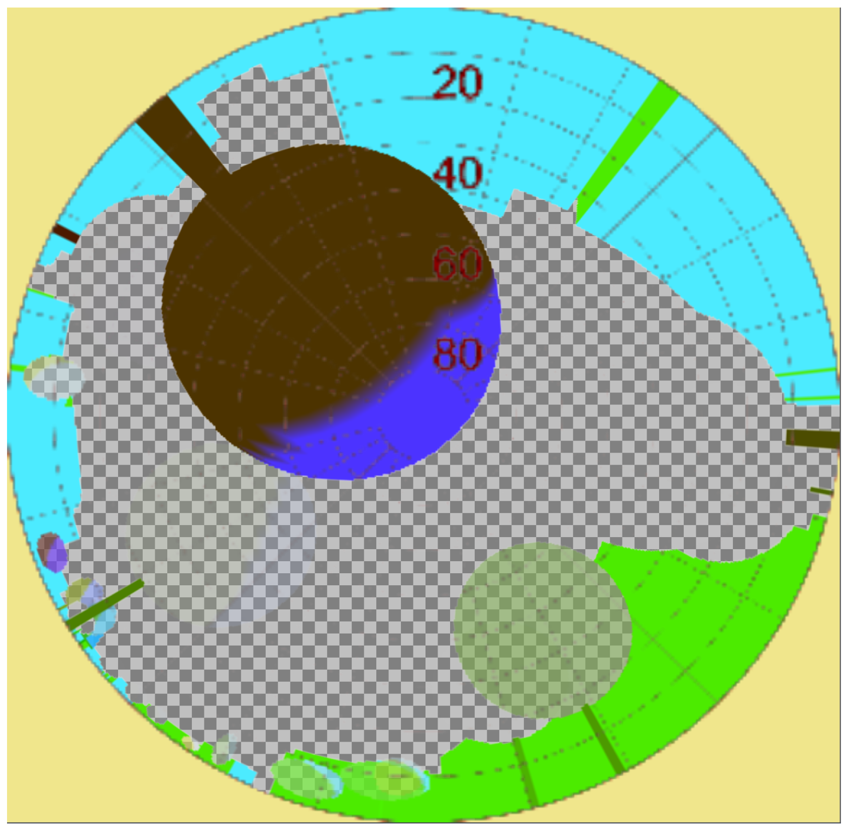
In contrast to most other models, the SkyHelios model does not consider the urban surroundings in terms of different surfaces, but in terms of pixels in the fisheye image (compare to Figure 1) weighted by the sine of the distance to the images center. Other parameters like the incident diffuse shortwave radiation at a specific location are estimated for the upper hemisphere at once.

2.1.1. Sky View Factor

All radiation calculations in SkyHelios are based on the local sky view factor (SVF). SVF is the fraction of the visible sky, seen from a certain point ([27], p. 353). It is dimensionless and ranges from 0 to 1, where 0 means that the sky is totally covered by terrain or obstacles, while 1 stands for a free sky. In SkyHelios, first, a fisheye image is rendered for the current location and elevation by the graphics engine (e.g., Figure 1). SVF is determined by distinguishing transparent and colored pixels in the image. Transparent pixels are counted as free sky, while all others are considered as covered by obstacles.

As in the real environment, the Fish-eye is a half-sphere, not all of the pixels should have the same influence on the SVF. Therefore, a dimensionless weighting factor ${\omega }_{proj}$ (Equation (1)) is used to consider the projection that adjusts the impact of a pixel by the sine of the zenith angle $\phi$ (${}^{\circ }$)

$${\omega }_{proj}=sin\left(\phi \right)·{\left(\frac{\phi }{{90}^{\circ }}\right)}^{-1}.$$

(1)

This results in a spheric SVF. If the planar SVF is desired, another correction by ${\omega }_{planar}$ (dimensionless) needs to be performed (compare to Equation (2)). It increases the impact of objects close to the ground by the cosine of the azimuth angle (counted from the ground to the top):

$${\omega }_{planar}={\omega }_{proj}·cos\left(\phi \right).$$

(2)

The accuracy of the sky view factor calculations has been assessed by [28].

2.1.2. Shortwave Radiation

Global radiation (G) consists of the direct solar irradiation (I) and the diffuse shortwave irradiation (D) ([26,27], p. 14) (all energy flux densities in $\frac{W}{m^2}$). Both of them are dependent on several parameters and therefore need to be modeled individually.

For a perfect clear sky condition (with no clouds and no horizon limitation), G can be calculated directly using Equation (3) proposed by [10,29,30]. In SkyHelios, Equation (3) is also used to derive an initial global radiation ($G_0$):

$$G_0=0.84·I_0·cos\left(\phi \right)·e^{\left(\frac{-0.027·\frac{pr}{p{r}_0}·T_L}{cos\left(\phi \right)}\right)}.$$

(3)

Equation (3) requires the initial direct solar radiation $I_0$, an energy flux density in $\frac{W}{m^2}$, the solar zenith angle $\phi$ (${}^{\circ }$), the actual air pressure $pr$ in hPa, as well as the one at sea level for a standard atmosphere ($p{r}_0$ = 1013 hPa) and the Linke turbidity factor $T_L$.

Direct Shortwave Irradiation

According to [29], I can be estimated as a function of $I_0$ ($\frac{W}{m^2}$), $\phi$ (${}^{\circ }$), $T_L$ (dimensionless), the relative optical air mass $r_{opt}$ (dimensionless), the vertical optical thickness of a standard atmosphere ${\delta }_{opt}$ (dimensionless as well), $pr$ in hPa, and cloud cover $cc$ in octas (0 = clear sky to 8 = overcast sky, Equation (4)):

$$I=I_0·cos\left(\phi \right)·e^{\left(-T_L·{\delta }_{opt}·r_{opt}·\frac{p}{p_0}\right)}·\left(1-\frac{cc}{8}\right).$$

(4)

This of course only holds for unshaded conditions. Under shaded conditions, I is usually assumed to equal 0 $\frac{W}{m^2}$.

The relative optical air mass ($r_{opt}$) can be estimated by (Equation (5)) [31].

$$r_{opt}={\left(sin\left({\beta }_s\right)+0.50572·{({\beta }_s+{6.07995}^{\circ })}^{-1.6364}\right)}^{-1}.$$

(5)

In Equation (5), ${\beta }_s$ describes the solar elevation angle in ${}^{\circ }$. Using ${\beta }_s$ and $r_{opt}$, ${\delta }_{opt}$ can be estimated following an approach by (Equation (6)) [32]:

$${\delta }_{opt}=\frac{1}{0.6·r_{opt}+9.4}.$$

(6)

Direct shortwave reflections by the surrounding obstacles are considered evaluating the surfaces lighting factor in terms of the blue channel of the fisheye image (compare to Figure 1). The reflection is estimated for any pixel in the fisheye as the blue color value (considering the orientation of the sun to the target surface) times the direct shortwave incident radiation and is considered to be isotropic. The shortwave reflections are therefore not calculated directly as proposed by e.g., [33,34,35] for it is found to be too time-consuming at run-time, but abbreviated from the graphic engines scenes lighting algorithm results. The directional lighting of the scene thereby considers the orientation of any surface to the light source (the sun) as the cosine of the angle between light source direction (a vector into the sun) and the surfaces normal vector.

Diffuse Shortwave Irradiation

According to [36], D can also be calculated as the sum of isotropic ($D_{iso}$) and anisotropic diffuse radiation ($D_{aniso}$, both in $\frac{W}{m^2}$). The isotropic part can be calculated by Equation (7):

$$D_{iso}=(G_0-I_{clear})·\left(1-\frac{I_{clear}}{I_0·cos\left(\phi \right)}\right)·{\mathsf{\Psi }}_S.$$

(7)

This equation requires the direct solar irradiation assuming a clear sky with no clouds $I_{clear}$ ($\frac{W}{m^2}$). The anisotropic component $D_{aniso}$ ($\frac{W}{m^2}$, Equation (8)) can be approximated by a similar equation if the sun is visible:

$$D_{aniso}=(G_0-I_{clear})·\frac{I_{clear}}{I_0·cos\left(\phi \right)}.$$

(8)

For the case of the sun covered by horizon or obstacles, $D_{0,aniso}$ becomes $0\frac{W}{m^2}$.

For non clear sky conditions, a linear correction according to [36] can be applied (Equation (9)). It considers the cloud cover ($cc$) in octas:

$$D_0=D_{clear}·\left(1-\frac{cc}{8}\right)+D_{overcast}·\frac{cc}{8}.$$

(9)

For a completely covered sky ($cc=8/8$), Ref. [36] proposes a simplified equation:

$$D=0.28·G_0·{\mathsf{\Psi }}_S.$$

(10)

In that case, global radiation can be approximated by scaling the initial global radiation ($G_0$) by 0.28 and the local sky view factor (${\mathsf{\Psi }}_S$) [36].

Shortwave diffuse reflections are considered in SkyHelios by estimating the diffuse incident radiation based on Equations (7)–(10) and scattering it isotropical scaled by the surfaces albedo.

2.1.3. Longwave Radiation

All surfaces are emitting longwave radiation according to the Stefan–Boltzmann law. It is calculating the longwave radiation flux density $P_{lw}$ ($\frac{W}{m^2}$) emitted by a perfectly black radiator surface (s) at a given surface temperature $T_s$ (K). The Stefan–Boltzmann law is modified by including an emission coefficient ${ϵ}_{lw}$ (dimensionless, Equation (11)) to be able to apply for non-perfectly black surfaces ($ϵ\ne 1.0$), e.g., for humans with an ${ϵ}_{lw}$ of approximately 0.97 ([10,37], p. 151):

$$P_{lw}={ϵ}_{lw}·\sigma ·A_s·T_s^4.$$

(11)

Elements within the equation are the longwave radiation flux density $P_{lw}$ in $\frac{W}{m^2}$, the Stefan–Boltzmann constant of 5.67 $\times {10}^{-8}\frac{W}{m^2·K^4}$ ($\sigma$), the radiating surface area $A_s$ in $m^2$, and its surface temperature $T_s$ in K.

Equation (11) is the basis for the estimation of both the longwave emissions by the sky ($P_{lwA}$), as well as the surroundings. The downwards longwave radiation is calculated based on $T_a$ and a virtual surface area determined from $VP$ and modified by cloud cover ($cc$) if available (Equation (12)).

Finding the appropriate value for ${ϵ}_{lw}$ can get very hard when it comes to longwave irradiation emitted by the atmosphere [38]. While there are empirical values available for quite some time [39,40,41], the determination of ${ϵ}_{lw}$ for a cloudy sky remains quite complex [38,42,43,44]:

$$P_{lwA}=\sigma ·T_a^4·\left(0.82-0.25\times {10}^{-0.0945·VP}\right)·\left(1+0.21·{\left(cc·0.125\right)}^{2.5}\right).$$

(12)

The ${ϵ}_{lw}$ of the current surrounding urban structures (buildings, plants) is derived from the object’s color in the fisheye image (compare to Figure 1). The surface temperature is determined iteratively evaluating short- (direct and diffuse) and longwave radiational gain as well as longwave emissions. The local $T_a$ thereby serves as an initial guess. Soil heat flux is approximated to be 19% of the surfaces energy balance Q if Q ≥ 0.0$\frac{W}{m^2}$ . For cases with Q ≤ 0.0$\frac{W}{m^2}$, a negative ground heat flux of 0.32 · Q is considered (please refer to [26] for details).

2.1.4. Mean Radiant Temperature

The mean radiant temperature $T_{mrt}$ (${}^{\circ }$C) is one of the most important input parameters for all sophisticated thermal indices applied in human-biometeorology. It is an equivalent surface temperature, which summarizes the effect of all the different short- and longwave radiation fluxes [29,37,45,46].

$T_{mrt}$ is defined as the surface temperature of a perfectly black, isothermal surrounding environment, which leads to the same energy balance as the current environment [10,37,47,48].

In most occasions, $T_{mrt}$ is calculated by small scale models [17,25,26,49]. Calculations are generally based on the Stefan–Boltzmann law (Equation (11) (compare to Section 2.1.3)).

By including the shortwave radiation flux density $P_{sw,s}$ ($\frac{W}{m^2}$) calculated by the diffuse solar irradiation and the diffuse reflected global radiation $D_s$ ($\frac{W}{m^2}$) multiplied by the shortwave absorption coefficient (1.0-Albedo, ${\alpha }_{abs,s}$) into Equation (11), the total radiation flux density to and from a surface, $P_s$ ($\frac{W}{m^2}$), e.g., the human body can be calculated by Equation (13):

$$P_s=\sigma ·A_s·T_s^4+{\alpha }_{abs,s}·D_s.$$

(13)

Dividing the environment of a person p into a number n of isothermal surfaces i and considering a projection factor $Pr$ to correct the relative surface size of p and s as well as the clothing $clo$ of p, $T_{mrt}$ in $\frac{W}{m^2}$ can be calculated following the principle of equal radiation fluxes caused by the actual and the reference environment (Equation (14)):

$$\begin{array}{c}\hfill {ϵ}_{lw,p}·\sigma ·\left(T_{mrt}^4-T_{cl}^4\right)=\\ \hfill {\Sigma }_{i=1}^n\left({ϵ}_{lw,p}·{ϵ}_{lw,i}·\sigma ·T_{s,i}^4+{\alpha }_{abs,s,i}·D_{s,i}\right)·P{r}_{p,i}-{ϵ}_{lw,p}·\sigma ·T_{cl}^4.\end{array}$$

(14)

Solving Equation (14) for $T_{mrt}$ results in Equation (15), which is perfectly applicable by numerical micro scale models:

$$T_{mrt}={\left[{\Sigma }_{i=1}^n\left({ϵ}_{lw,i}·T_{s,i}^4+\frac{{\alpha }_{abs,s,i}·D_{s,i}}{{ϵ}_{lw,p}·\sigma }\right)·P{r}_{p,i}\right]}^{0.25}.$$

(15)

Most numerical models in urban biometeorology, however, are using further simplifications [17,25,26].

2.2. Wind Modeling

Wind data is estimated in SkyHelios based on a diagnostic wind model based on the principles by [50]. It considers up to four stream modifications for each individual obstacle. In agreement to [50], a upwind stagnation zone, a downwind recirculation, a downwind velocity deficite zone, as well as a street canyon vortex can be considered. However, updated parametrizations are implemented to allow for improved precision.

2.2.1. Upwind Stagnation Zone

For most obstacles, an upwind stagnation zone according to [51] is considered. The maximum windwards extension is determined by Equation (16):

$${\displaystyle \frac{L_f}{h}}={\displaystyle \frac{1.5\left(\frac{wi}{h}\right)}{1+0.8\left(\frac{wi}{h}\right)}}.$$

(16)

In Equation (16), $L_f$ describes the maximum windward extension of the stagnation zone, h is the obstacles height, and $wi$ stands for the obstacles width (all units in meters).

Ref. [51] also introduces a modified power law profile to determine the average wind speed component $\overline{u}$ (m/s) at any vertical level z for within the front eddy zone containing a factor that reduces the wind component perpendicular to the obstacle (compare to Equation (17)):

$$\frac{\overline{u}\left(z\right)}{u_h}=0.4·\left(\frac{z}{h}\right).$$

(17)

In addition, a vortex zone was included into the front eddy zone [51]. Its streamwise length $L_{fv}$ (m) is determined by Equation (18):

$${\displaystyle \frac{L_{fv}}{h}}={\displaystyle \frac{0.6\left(\frac{wi}{h}\right)}{1+0.8\left(\frac{wi}{h}\right)}}.$$

(18)

The ellipsoidal vortex zone is then filled by a parametrization gathered from fitting experimental wind-tunnel data [51]. The trigonometric Equations (19) and (20) are used to calculate the average vortex components in the horizontal ($\overline{u}$, Equation (19)) and the vertical ($\overline{w}$, Equation (20), both in the m/s) direction:

$$\frac{\overline{u}\left(z\right)}{u_h}=\left(0.6cos\left({\displaystyle \frac{\pi h_v}{0.5h}}\right)+0.05\right)·\left(-0.6sin\left({\displaystyle \frac{\pi l_v}{L_{fv}}}\right)\right),$$

(19)

$$\frac{\overline{w}\left(z\right)}{u_h}=-0.1·cos\left({\displaystyle \frac{\pi l_v}{L_{fv}}}\right)-0.05.$$

(20)

$l_v$ and $h_v$ are defined as the current length and height of the vortex in meters.

2.2.2. Downwind Recirculation Zone

Ref. [52] introduced an improved parametrizations for the velocity deficit zone in the lee of an obstacle. The shelter model by [52], which is also adopted in the QUICK-URB model calculates a Gaussian velocity deficit pattern using Equations (21)–(23):

$${\displaystyle \frac{u_d(x,y,z)}{U\left(H\right)}}=\mathsf{\Gamma }{C}_D\left({\displaystyle \frac{W}{H}}\right){\left({\displaystyle \frac{x}{H}}\right)}^{-1.5}F\left(\eta \right)G\left(\zeta \right),$$

(21)

$$F\left(\eta \right)={\left({\displaystyle \frac{1}{{\left(2\pi \right)}^{0.5}{a}_f}}\right)}^{\left({\displaystyle \frac{-{\eta }^2}{2a_f^2}}\right)},$$

(22)

$$G\left(\zeta \right)={\left(c_a\zeta \right)}^{\left(-a_g{\zeta }^{1.5}\right)}.$$

(23)

$u_d$ represents the velocity deficit in the lee of an obstacle in m/s, x, y, and z are the stream coordinates in x-, y-, and z-directions, W the width, and H the height of an obstacle in m, U(H) the mean wind speed at the top of the obstacle in m/s based on the upstream power law profile, and $C_D$ is the drag coefficient. $\mathsf{\Gamma }$ is defined as $0.6·c_a^2$. The similarity coordinates $\eta$, and $\zeta$, as well as the vertical coefficients $c_a$, and $a_g$ are calculated according to the following equations:

$$\eta =\left(\frac{z}{h}\right)·{\left(\frac{x}{h}\right)}^{-0.5},$$

(24)

$$\zeta =\left(\frac{y}{h}\right)·{\left(\frac{x}{h}\right)}^{-0.5},$$

(25)

$$c_a=\sqrt{{\displaystyle \frac{\left({\displaystyle \frac{ln(h+z_0)}{z_0}}\right)}{2·{\kappa }^2}}},$$

(26)

$$a_g=0.8·c_a^{1.5}.$$

(27)

$\kappa$ in Equation (26) is the von Kármán constant of 5.67 ×${10}^{-8}\frac{W}{m^2·T_s^4}$.

The main advantage of the integration of the shelter model by [52] is the streamwise velocity deficits that can be calculated more accurately than by the original parametrization [53].

2.2.3. Street Canyon Parametrization

As a response to the overestimation of the width of a street canyon vortex by the original parametrization (compare to [54]), a modified street canyon model was implemented in SkyHelios. One significant difference to the original parametrization according to [50] is the transition zone at the ends of the vortex formed by vertical wedges.

The vertical wedges are modified after Equation (28), where $d_{sc}$ represents the distance of a point to the upwind obstacle (in meters) and $u_{rt}$ the wind speed component in rooftop height (m/s):

$$\frac{u^0}{u_{rt}}={\displaystyle \frac{tanh\left(\frac{0.2·d_{sc}-h}{0.2·d_{sc}}\right)}{tanh\left(1\right)}}.$$

(28)

In addition, the criteria to detect a street canyon has been modified according to [54]. It is now based on the length of the upstream obstacles recirculation zone ($L_R$). Whether a street canyon is set or not is distinguished according to Equation (29). l represents the obstacles streamwise length:

$$\frac{L_R}{h}={\displaystyle \frac{1.8·\frac{wi}{h}}{{\left(\frac{l}{h}\right)}^{0.3}\left(1+0.24·\frac{wi}{h}\right)}}.$$

(29)

For the central part of a street canyon, Ref. [54] proposes a streamwise speed modification according to Equation (30):

$$\frac{u^0}{u_{rt}}=-0.3·\frac{d_{nW}}{0.5·d_{SCw}}·\left(\frac{d_{SCw}-d_{nW}}{0.5·d_{SCw}}\right)·F_{SC}.$$

(30)

Equation (30) calculates the street canyon modification from the distance to next wall $d_{nw}$, the street canyon width $d_{SCw}$ (both in meters) and the function $F_{SC}$, stated by Equation (31):

$$F_{SC}={\left(1.0-0.5·\frac{|d_{SCccw}|}{wi-2.0·(0.2·d_{nw})}\right)}^{0.25}.$$

(31)

The only new parameter in Equation (31) is the crosswind distance to the street canyons center $d_{SCccw}$ in m.

For further details on the parametrizations, please see [55].

The wind field calculated by the given functions most likely contains some divergence. Assuming incompressible air, this divergence has to be minimized in order to get a valid wind field. Mathematically, this is performed by minimizing the functional for the scalar H in Equation (32):

$$\begin{array}{c}\hfill H(u,v,w)=\\ \hfill \int \int \int \left({\alpha }_h^2{(u-u^0)}^2+{\alpha }_h^2{(v-v^0)}^2+{\alpha }_v^2{(w-w^0)}^2\right)dxdydz.\end{array}$$

(32)

In Equation (32), ${\alpha }_h$ and ${\alpha }_v$ are horizontal stability factors in s/m, u, v and w are the stream components in m/s, $u^0$, $v^0$ and $w^0$ are representing the initial stream components in m/s while $dx$, $dy$ and $dz$ are the grid spacings in m.

2.3. Area of Interest and Data

The advanced SkyHelios model is tested for two study areas in Freiburg, southwest Germany (approximately 47${}^{\circ }$59${}^{\prime }$ N, 7${}^{\circ }$51${}^{\prime }$ E). The place of the old synagogue is located westwards from the inner city of Freiburg between the main university buildings I and II (KG I and KG II), the university library and the theater (compare to Figure 2, bottom left). The Institutes Quarter is a city quarter north of the city center mainly consisting of institute buildings of the Albert-Ludwigs-University Freiburg. It covers an area of approximately 700 m on 500 m (compare to Figure 2, top right).

At the place of the old synagogue, some tree information is also available. The point-feature shapefile available consists of 21 trees. To test the radiation calculation capabilities of the SkyHelios model, the attribute fields “opticalDen”, “albedo”, and “emissivity” (for the optical density, surface albedo and surface emission coefficient) have been assigned arbitrary values in a wide range. For example, the optical density ranges from 0.06 to 1.0, where 0 is transparent and 1 is opaque.

The urban climate station Freiburg, a meteorological background station [56] at the top of a highrise building within the “Institutes Quarter” provides data that can be used as a roof-top reference. The stations records are covering a 13-year period from 1 September 1999 to 30 April 2013 in hourly resolution. The parameters used in this study are air temperature ($T_a$) in ${}^{\circ }$C, vapour pressure ($VP$) in hPa, global radiation (G) in $\frac{W}{m^2}$, wind speed (v) in m/s and wind direction ($WD$) in ${}^{\circ }$.

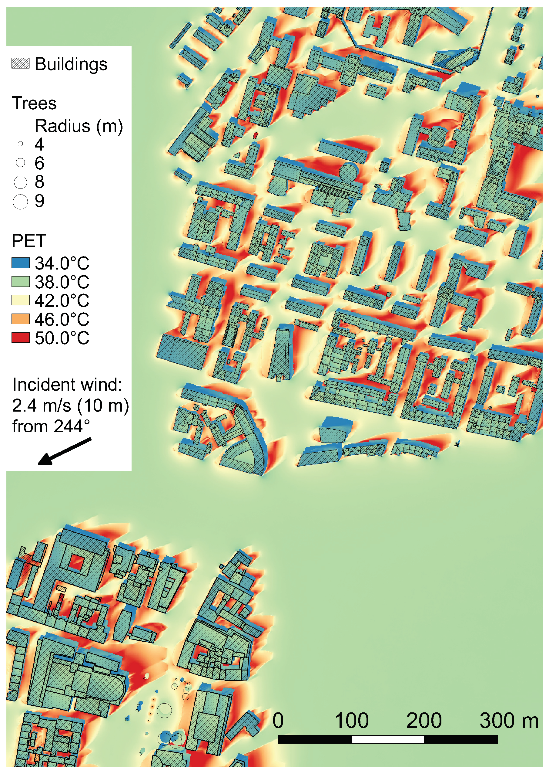
To keep it short, only results for the 1 July 2008 at 1:30 p.m. local standard time are presented here. The 1st of July 2008 was a clear summer day with $T_a$ of 28.2 ${}^{\circ }$C, vapour pressure of 17.8 hPa, an incident wind speed of 2.4 m/s in 10 m height from 244${}^{\circ }$ and global radiation of 887$\frac{W}{m^2}$ at 1:30 p.m.

3. Results and Discussion

In spite of there being a lot of results generated during this study, only some of them are presented here. However, the selected results are sufficient for the identification of the most appropriate shading type in terms of reduction of heat stress as well as for demonstrating the capabilities of the advanced SkyHelios model. For a spatial result, the example of PET in a height of 1.1 m on 1 July 2008 at 1:30 p.m. LST (Figure 3) was selected. The index is strongly influenced by both radiation and wind speed [6,57] and thus shows the impact of both.

Looking at Figure 3, the strongest reduction of PET by approximately 8.0 ${}^{\circ }$C (compared to PET 38.3 ${}^{\circ }$C at undisturbed locations) can be found in locations shaded by solid obstacles (mostly buildings). This is mainly caused by a reduction in $T_{mrt}$ of almost 22.5 ${}^{\circ }$C due to the obstacles blocking direct solar radiation. Global radiation is reduced by around 650$\frac{W}{m^2}$. This is in quite good agreement with studies for summer days in Freiburg, e.g., [58]. Obstacles with transparency are causing a slighter reduction. For example, the trees with an optical density of 0.8 are reducing PET by approx. 6.3 ${}^{\circ }$C, those with an optical density of 0.6 are causing a reduction of 5.4 ${}^{\circ }$C. Global radiation is reduced from 857$\frac{W}{m^2}$ in unshaded locations to 393 $\frac{W}{m^2}$ and 334$\frac{W}{m^2}$ in the same locations, respectively. The effect on PET thereby strongly depends on wind speed. During a measurement campaign in August 2007, a measuring point below a tree was found to be 4.6 ${}^{\circ }$C (PET) cooler on average than one not located below a tree [59]. However, as the shortwave transitivity of the tree is unknown, wind speed is slightly higher and radiation fluxes within complex urban environments are generally quite inhomogeneous in space, results are hard to compare. This is also shown by a PET reduction of 3.0 to almost 10.0 ${}^{\circ }$C was found comparing a measurement point under a tree with four other ones without trees for the 2nd of August 2001 in Freiburg [25]. However, that study applied the RayMan model, which does not account for transparency. In a significantly warmer setting, Ref. [60] found a reduction in PET of up to 15.6 ${}^{\circ }$C due to (solid) trees for a summer case in Lisbon. The dependence of the reduction on general thermal conditions is indicated by the maximum reduction found for winter conditions was 2.7 ${}^{\circ }$C in the same study [60].

Wind speed in the model domain was quite low within the whole model domain at 1:30 p.m. on the 1st of July 2008 with only 2.4$\frac{m}{s}$ in a height of 10 m above ground level. This causes even lower wind speed at pedestrian level (1.1 m above ground) where wind speed was reduced to 0.9$\frac{m}{s}$ in (spatial, arithmetic) average. However, this comprises wind speed in locations without obstacles input (in the northwest and in the southeast of the combined domain where wind speed is approximately 1.4$\frac{m}{s}$ constantly. Wind speed therefore is mostly found to be lower close to the obstacles, but can also be increased due to corner flow and channeling to up to 3.8$\frac{m}{s}$ in some locations. It thereby needs to be noted that wind speed (in the height of 1.1 m) is only slightly decreased by most of the trees. Only the small trees (e.g., in the center of the Place of the Old Synagogue) cause a stronger reduction in wind speed of around 0.1$\frac{m}{s}$ at that level. However, in some locations, an increase by the same amount can be found due to the air current avoiding the tree crown.

Increased wind speed at building corners does reduce PET by up to 2.0 ${}^{\circ }$C in the results. Stagnation caused by buildings, on the other hand, does lead to an increase in PET of up to 15.4 ${}^{\circ }$C in this example. Both effects are clearly present in the results. However, the reduction of PET by increased wind speed can only be found in quite small areas, while low wind speed increases PET in rather large areas (almost all the red areas in Figure 3 are caused by low wind speed).

In spite of the size and the high resolution of the model domain, the model run time of almost one hour on a below average machine can be considered to be quite fast (e.g., compared to the prognostic model ENVI-met [15]). However, to the authors’ knowledge, there is currently no other model available that can calculate similar results for a domain size and resolution considered in this study. The model performance in terms of computation time can therefore hardly be compared.

The low computational effort is partly by utilizing the graphics hardware, but also due to the diagnostic model design that allows for avoiding solving transport equations. This comes at the price of unknown previous conditions resulting in e.g., ground or wall heat storage can only be parameterized assuming rather constant conditions. This will e.g., lead to an underestimation in surface temperature in the time after sunset [26].

Some parts of the advanced SkyHelios model have been validated in the past (e.g., the SVF model [28]). Other parts do equal those of the very well validated RayMan model (e.g., the radiation model without the reflections part [25,26]). Furthermore, the results generated by the advanced SkyHelios model are generally plausible and in basic agreement to findings by other studies (e.g., [6,61,62,63]). However, further validation of the whole model and comparison to on-site measurements is required to assess the model’s accuracy.

4. Conclusions

Results show that heat stress for humans in urban areas can best be prevented by providing shading and, at the same time, not reducing wind speed too much. While buildings are solid obstacles in terms of radiation and therefore can provide more comfortable conditions in the shade, they are solid obstacles to wind at the same time. This mostly causes a reduction in wind speed leading to more uncomfortable conditions. The most comfortable conditions can be found below the trees. They are providing shade and are hardly causing wind speed reductions at the pedestrian level. This of course only holds as long as they are large enough (the small trees in the center of the place of the old synagogue are hardly casting any shadow, but are causing wind sheltering as the crowns are only slightly above the pedestrian level) and as long their crowns are dense enough. The most suitable shading type is therefore found to be provided by individual large trees with dense crowns.

The advanced SkyHelios model is capable of estimating wind speed and -direction, the mean radiant temperature, as well as the thermal indices PT, UTCI, and PET for large areas of interest in high resolution as shown by the results. This allows for analyzing larger areas of interest in more detail by using average office computers, which makes it a very valuable tool for all users working on spatial and temporal dimensions in the field of human thermal biometeorology.

References

- Matzarakis, A.; Muthers, S.; Koch, E. Human-biometeorological evaluation of summer mortality in Vienna. Theor. Appl. Climatol. 2011, 105, 1–10. [Google Scholar] [CrossRef]
- Ketterer, C.; Matzarakis, A. Comparison of Different Methods for the Assessment of the Urban Heat Island in Stuttgart, Germany. Int. J. Biometeorol. 2015, 59, 1299–1309. [Google Scholar] [CrossRef] [PubMed]
- Fröhlich, D.; Matzarakis, A. Modeling of changes in human thermal bioclimate resulting from changes in urban design—Examples based on a popular place in Freiburg, SW-Germany. In Proceedings of the MettoolsVIII, 8. Fachtagung des Ausschusses Umweltmeteorologie der Deutschen Meteorologischen Gesellschaft, Leipzig, Germany, 20–22 March 2012; pp. 1–8. [Google Scholar]
- Lopes, A.; Lopes, S.; Matzarakis, A.; Alcoforado, M.J. The influence of the summer sea breeze on thermal comfort in Funchal (Madeira). A contribution to tourism and urban planning. Meteorol. Z. 2011, 20, 553–564. [Google Scholar] [CrossRef]
- Lin, T.P.; Matzarakis, A.; Hwang, R.L. Shading effect on long-term outdoor thermal comfort. Build. Environ. 2010, 45, 213–221. [Google Scholar] [CrossRef]
- Hwang, R.L.; Lin, T.P.; Matzarakis, A. Seasonal effects of urban street shading on long-term outdoor thermal comfort. Build. Environ. 2011, 46, 863–870. [Google Scholar] [CrossRef]
- Fröhlich, D.; Matzarakis, A. Modeling of changes in thermal bioclimate: Examples based on urban spaces in Freiburg, Germany. Theor. Appl. Climatol. 2013, 111, 547–558. [Google Scholar] [CrossRef]
- Lin, T.P.; Tsai, K.T.; Liao, C.C.; Huang, Y.C. Effects of thermal comfort and adaptation on park attendance regarding different shading levels and activity types. Build. Environ. 2013, 59, 599–611. [Google Scholar] [CrossRef]
- Charalampopoulos, I.; Tsiros, I.; Chronopoulou-Sereli, A.; Matzarakis, A. A note on the evolution of the daily pattern of thermal comfort-related micrometeorological parameters in small urban sites in Athens. Int. J. Biometeorol. 2015, 59, 1223–1236. [Google Scholar] [CrossRef] [PubMed]
- VDI. VDI Guideline 3787, Part 2: Environmental Meteorology. Methods for the Human Biometeorological Evaluation of Climate and Air Quality for Urban and Regional Planning at Regional Level. Part I: Climate; Technical Report 1b; VDI: Düsseldorf, Germany, 2008. [Google Scholar]
- Herrmann, J.; Matzarakis, A. Mean radiant temperature in idealized urban canyons—Examples from Freiburg, Germany. Int. J. Biometeorol. 2012, 56, 199–203. [Google Scholar] [CrossRef] [PubMed]
- Lin, T.P.; Matzarakis, A.; Hwang, R.L.; Huang, Y.C. Effect of pavements albedo on long-term outdoor thermal comfort. In Proceedings of the 7th Conference on Biometeorology, Freiburg, Germany, 12–14 April 2010; Volume 20, pp. 498–504. [Google Scholar]
- Shashua-Bar, L.; Pearlmutter, D.; Erell, E. The influence of trees and grass on outdoor thermal comfort in a hot-arid environment. Int. J. Climatol. 2011, 31, 1498–1506. [Google Scholar] [CrossRef]
- Bruse, M.; Fleer, H. Simulating surface–plant–air interactions inside urban environments with a three dimensional numerical model. Environ. Model. Softw. 1998, 13, 373–384. [Google Scholar] [CrossRef]
- Bruse, M. Die Auswirkungen Kleinskaliger Umweltgestaltung auf das Mikroklima. Entwicklung des Prognostischen Numerischen Modells ENVI-met zur Simulation der Wind-, Temperatur- und Feuchteverteilung in StäDtischen Strukturen. Ph.D. Thesis, Ruhr-Universität Bochum, Bochum, Germany, 1999. [Google Scholar]
- Lindberg, F.; Grimmond, C.S.B.; Gabey, A.; Huang, B.; Kent, C.W.; Sun, T.; Theeuwes, N.E.; Jarvi, L.; Ward, H.C.; Capel-Timms, I.; et al. Urban Multi-scale Environmental Predictor (UMEP): An integrated tool for city-based climate services. Environ. Model. Softw. 2018, 99, 70–87. [Google Scholar] [CrossRef]
- Lindberg, F.; Holmer, B.; Thorsson, S. SOLWEIG 1.0—Modelling spatial variations of 3D radiant fluxes and mean radiant temperature in complex urban settings. Int. J. Biometeorol. 2008, 52, 697–713. [Google Scholar] [CrossRef] [PubMed]
- Matzarakis, A.; Matuschek, O. Sky view factor as a parameter in applied climatology—Rapid estimation by the SkyHelios model. Meteorol. Z. 2011, 20, 39–45. [Google Scholar] [CrossRef]
- Staiger, H.; Laschewski, G.; Graetz, A. The perceived temperature - a versatile index for the assessment of the human thermal environment. Part A: Scientific basics. Int. J. Biometeorol. 2012, 56, 165–176. [Google Scholar] [CrossRef] [PubMed]
- Jendritzky, G.; de Dear, R.; Havenith, G. UTCI-Why another thermal index? Int. J. Biometeorol. 2012, 421–428. [Google Scholar] [CrossRef] [PubMed] [Green Version]
- Bröde, P.; Fiala, D.; Blazejczyk, K.; Holmér, I.; Jendritzky, G.; Kampmann, B.; Tinz, B.; Havenith, G. Deriving the operational procedure for the Universal Thermal Climate Index (UTCI). Int. J. Biometeorol. 2012, 56, 481–494. [Google Scholar] [CrossRef] [PubMed] [Green Version]
- Höppe, P.R. The physiological equivalent temperature—A universal index for the biometeorological assessment of the thermal environment. Int. J. Biometeorol. 1999, 43, 71–75. [Google Scholar] [CrossRef] [PubMed]
- MOGRE Community. Managed Open Graphics Rendering Engine; MOGRE Community, 2016; Available online: http://wiki.ogre3d.org/MOGRE (accessed on 18 November 2017).
- Open Source Geospatial Foundation. GDAL/OGR Geospatial Data Abstraction Software Library; Open Source Geospatial Foundation, 2018; Available online: http://gdal.org (accessed on 18 March 2018).
- Matzarakis, A.; Rutz, F.; Mayer, H. Modelling radiation fluxes in simple and complex environments—Application of the RayMan model. Int. J. Biometeorol. 2007, 51, 323–334. [Google Scholar] [CrossRef] [PubMed]
- Matzarakis, A.; Rutz, F.; Mayer, H. Modelling radiation fluxes in simple and complex environments: Basics of the RayMan model. Int. J. Biometeorol. 2010, 54, 131–139. [Google Scholar] [CrossRef] [PubMed]
- Oke, T.R. Boundary Layer Climates, 2nd ed.; Routledge: London, UK; New York, NY, USA, 1995. [Google Scholar]
- Hämmerle, M.; Gál, T.; Unger, J.; Matzarakis, A. Comparison of models calculating the Sky View Factor used for urban climate investigations. Theor. Appl. Climatol. 2011, 105, 521–527. [Google Scholar] [CrossRef]
- Jendritzky, G.; Menz, H.; Schirmer, H.; Schmidt-Kessen, W. Methodik zur Raumbezogenen Bewertung der Thermischen Komponente im Bioklima des Menschen (Fortgeschriebenes Klima-Michel-Modell); Akad für Raumforschung und Landesplanung: Hannover, Germany, 1990. [Google Scholar]
- VDI. VDI Guideline 3789, Part 1: Climate. Environmental Meteorology, Interactions between Atmosphere and Surface; Calculation of Short-and Long Wave Radiation. Part 2: VDI/DIN-Handbuch Reinhaltung der Luft; Technical Report 1b; VDI: Düsseldorf, Germany, 1994. [Google Scholar]
- Kasten, F.; Young, A. Revised optical air-mass tables and approximation formula. Appl. Opt. 1989, 28, 4735–4738. [Google Scholar] [CrossRef] [PubMed]
- Kasten, F. A simple parametrization of the pyrheliometric formula for determining the linke turbidity factor. Meteorol. Rundsch. 1980, 33, 124–127. [Google Scholar]
- Krayenhoff, E.S.; Voogt, J.A. A microscale three-dimensional urban energy balance model for studying surface temperatures. Bound.-Layer Meteorol. 2007, 123, 433–461. [Google Scholar] [CrossRef]
- Yang, X.; Li, Y. Development of a Three-Dimensional Urban Energy Model for Predicting and Understanding Surface Temperature Distribution. Bound.-Layer Meteorol. 2013, 149, 303–321. [Google Scholar] [CrossRef]
- Resler, J.; Krč, P.; Belda, M.; Juruš, P.; Benešová, N.; Lopata, J.; Vlček, O.; Damašková, D.; Eben, K.; Derbek, P.; et al. PALM-USM v1.0: A new urban surface model integrated into the PALM large-eddy simulation model. Geosci. Model Dev. 2017, 10, 3635–3659. [Google Scholar] [CrossRef]
- Valko, P. Die Himmelsstrahlung in ihrer Beziehung zu verschiedenen Parametern. Arch. Meteorol. Geophys. Bioklimatol. Ser. B 1966, 14, 336–359. [Google Scholar] [CrossRef]
- Fanger, P. Thermal Comfort; McGraw-Hill: New York, NY, USA, 1972. [Google Scholar]
- Staiger, H.; Matzarakis, A. Evaluation of atmospheric thermal radiation algorithms for daylight hours. Theor. Appl. Climatol. 2010, 102, 227–241. [Google Scholar] [CrossRef]
- Brunt, D. Notes on radiation in the atmosphere. I. Q. J. R. Meteorol. Soc. 1932, 58, 389–420. [Google Scholar] [CrossRef]
- Swinbank, W.C. Long-wave radiation from clear skies. Q. J. R. Meteorol. Soc. 1963, 89, 339–348. [Google Scholar] [CrossRef]
- Satterlund, D. Improved equation for estimating long-wave-radiation from the atmosphere. Water Resour. Res. 1979, 15, 1649–1650. [Google Scholar] [CrossRef]
- Crawford, T.M.; Duchon, C.E. An Improved Parameterization for Estimating Effective Atmospheric Emissivity for Use in Calculating Daytime Downwelling Longwave Radiation. J. Appl. Meteorol. 1999, 38, 474–480. [Google Scholar] [CrossRef]
- Iziomon, M.G.; Mayer, H.; Matzarakis, A. Downward atmospheric longwave irradiance under clear and cloudy skies: Measurement and parameterization. J. Atmos. Sol.-Terr. Phys. 2003, 65, 1107–1116. [Google Scholar] [CrossRef]
- Duarte, H.F.; Dias, N.L.; Maggiotto, S.R. Assessing daytime downward longwave radiation estimates for clear and cloudy skies in Southern Brazil. Agric. For. Meteorol. 2006, 139, 171–181. [Google Scholar] [CrossRef]
- Kantor, N.; Unger, J. The most problematic variable in the course of human-biometeorological comfort assessment—The mean radiant temperature. Cent. Eur. J. Geosci. 2011, 3, 90–100. [Google Scholar] [CrossRef] [Green Version]
- Chen, Y.C.; Lin, T.P.; Matzarakis, A. Comparison of mean radiant temperature from field experiment and modelling: A case study in Freiburg, Germany. Theor. Appl. Climatol. 2014, 118, 535–551. [Google Scholar] [CrossRef]
- Der Luft, V.K.R. Stadtklima und Luftreinhaltung: Ein Wissenschaftliches Handbuch für die Praxis in der Umweltplanung; mit 47 Tabellen; Technical Report; Springer: Berlin/Heidelberg, Germany, 1988. [Google Scholar]
- Helbig, A.; Baumüller, J.; Kerschgens, M.J. Stadtklima und Luftreinhaltung. 2., VollstäNdig üBerarbeitete und ErgäNzte Auflage mit 200 Abbildungen und 79 Tabellen, 2th ed.; Springer: Berlin/Heidelberg, Germany, 1999. [Google Scholar]
- Matzarakis, A. Die thermische Komponente des Stadtklimas; Number 6 in Berichte des Meteorologischen Institutes der Universität Freiburg; Meteorologisches Inst.: Freiburg, Germany, 2001. [Google Scholar]
- Röckle, R. Bestimmung der Strömungsverhältnisse im Bereich Komplexer Bebauungsstrukturen. Ph.D. Thesis, Fachbereich Mechanik der Technischen Hochschule Darmstadt, Darmstadt, Germany, 1990. [Google Scholar]
- Bagal, N.; Pardyjak, E.; Brown, M. Improved Upwind Cavity Parameterizations for a Fast Response Urban Wind Model. In Proceedings of the AMS Symposium on Planning, Nowcasting, and Forecasting in the Urban Zone, Seattle, WA, USA, 11–15 January 2004. [Google Scholar]
- Taylor, P.A.; Salmon, J.R. A model for the correction of surface wind data for sheltering by upwind obstacles. J. Appl. Meteorol. 1993, 49, 226–239. [Google Scholar] [CrossRef]
- Pardyjak, E.R.; Brown, M.J.; Bagal, N. Improved Velocity Deficit Parameterizations for a Fast Response Urban Wind Model. In Proceedings of the AMS Symposium on Planning, Nowcasting, and Forecasting in the Urban Zone, Seattle, WA, USA, 11–15 January 2004. [Google Scholar]
- Singh, B.; Hansen, B.S.; Brown, M.J.; Pardyjak, E.R. Evaluation of the QUIC-URB fast response urban wind model for a cubical building array and wide building street canyon. Environ. Fluid Mech. 2008, 8, 281–312. [Google Scholar] [CrossRef]
- Fröhlich, D. Development of a Microscale Model for the Thermal Environment in Complex Areas. Ph.D. Thesis, Albert-Ludwigs-Universität, Freiburg, Germany, 2017. [Google Scholar] [CrossRef]
- Matzarakis, A.; Mahlau, F.; Mayer, H. Online-visualisierung von meteorologischen Daten im Internet—Meteorologische Stadtstation Freiburg. In Proceedings of the Fachtagung Mettools IV, Bonn, Germany, 4–6 October 2000; pp. 150–152. [Google Scholar]
- Emmanuel, R.; Johansson, E. Influence of urban morphology and sea breeze on hot humid microclimate: The case of Colombo, Sri Lanka. Clim. Res. 2006, 30, 189–200. [Google Scholar] [CrossRef]
- Matzarakis, A.; Mayer, H.; Iziomon, M.G. Applications of a universal thermal index: Physiological equivalent temperature. Int. J. Biometeorol. 1999, 43, 76–84. [Google Scholar] [CrossRef] [PubMed]
- Mayer, H.; Kuppe, S.; Holst, J.; Imbery, F. Human thermal comfort below the canopy of street trees on a typical Central European summer day. In Proceedings of the 5th Japanese-German Meeting on Urban Climatology, Freiburg, Germany, 6–8 October 2008; in Number 18 in Berichte des Meteorologischen Institutes der Universität Freiburg; Meteorologisches Inst.: Freiburg, Germany, 2009; pp. 211–219. [Google Scholar]
- Nouri, A.S.; Fröhlich, D.; Silva, M.M.; Matzarakis, A. The Impact of Tipuana tipu Species on Local Human Thermal Comfort Thresholds in Different Urban Canyon Cases in Mediterranean Climates: Lisbon, Portugal. Atmosphere 2018, 9, 12. [Google Scholar] [CrossRef]
- Mayer, H.; Holst, J.; Dostal, P.; Imbery, F.; Schindler, D. Human thermal comfort in summer within an urban street canyon in Central Europe. Meteorol. Z. 2008, 17, 241–250. [Google Scholar] [CrossRef]
- De Abreu-Harbicha, L.V.; Labakia, L.C.; Matzarakis, A. Effect of tree planting design and tree species on human thermal comfort in the tropics. Landsc. Urban Plan. 2015, 138, 99–109. [Google Scholar] [CrossRef]
- Fröhlich, D.; Matzarakis, A. A quantitative sensitivity analysis on the behaviour of common thermal indices under hot and windy conditions in Doha, Qatar. Theor. Appl. Climatol. 2016, 124, 179–187. [Google Scholar] [CrossRef]
Figure 1.
Fisheye image showing the upper hemisphere with trees and buildings as generated by the SkyHelios model in production mode. The colors and opacity correspond to different shortwave albedo, longwave emissivity, direct radiation factor of the surfaces (including direct shortwave reflections). The checkerboard background was added to visualize the objects opacity.
Figure 2.
Screenshot of SkyHelios main window showing a combined model domain consisting of two areas of interest in Freiburg, Southwest Germany: the “Institutes Quarter” and the “Place of the Old Synagogue”.
Figure 3.
Physiologically Equivalent Temperature (PET) on 1 July 2008 at 1:30 p.m. in a height of 1.1 m above ground level. The calculations consider both the “Institutes Quarter” (upper right) and the “Place of the Old Synagogue” (lower left) together in one large area of interest.
© 2018 by the authors. Licensee MDPI, Basel, Switzerland. This article is an open access article distributed under the terms and conditions of the Creative Commons Attribution (CC BY) license (http://creativecommons.org/licenses/by/4.0/).
Share and Cite
MDPI and ACS Style
Fröhlich, D.; Matzarakis, A. Spatial Estimation of Thermal Indices in Urban Areas—Basics of the SkyHelios Model. Atmosphere 2018, 9, 209. https://doi.org/10.3390/atmos9060209
AMA Style
Fröhlich D, Matzarakis A. Spatial Estimation of Thermal Indices in Urban Areas—Basics of the SkyHelios Model. Atmosphere. 2018; 9(6):209. https://doi.org/10.3390/atmos9060209
Chicago/Turabian StyleFröhlich, Dominik, and Andreas Matzarakis. 2018. "Spatial Estimation of Thermal Indices in Urban Areas—Basics of the SkyHelios Model" Atmosphere 9, no. 6: 209. https://doi.org/10.3390/atmos9060209
Note that from the first issue of 2016, this journal uses article numbers instead of page numbers. See further details here.